1. Introduction
During the past three decades, with important changes in its economy and social structure, China has experienced a major demographic transition of rapid and intense urbanization [
1,
2]. From 1985 to 2012, the level of urbanization in China grew by 221% [
3]. During the same period, the level of motorization boomed at 19% annually [
3], while non-motorized transportation declined and public transportation continued to develop slowly. Currently, travel and transportation in Chinese cities is developing from a once “bicycle-dominated” mode split [
1] to a more motorized one. For example, from 1995 to 2009, the household vehicle (car and motorcycle) trips of Shanghai, the largest city in China, increased by 2.5 times to nearly 1.5 trips per day, despite the government’s endeavor to promote public transport. Similarly, in the Zhongshan Metropolitan Area study case, the average household vehicle trip grew from 1.7 trips per day to 2.8 in merely seven years (2003 to 2009). This situation has contributed to China’s increasingly severe urban traffic and environmental problems, which are spreading from big cities to medium-sized cities. How does one slow down and even reduce the fast-growing vehicle use during rapid motorization and promote sustainable transportation? This has become a challenge for planners, scholars and policy makers throughout China. In the past decade, policy makers in China have gradually recognized the effects of planning policies involving the built environment through the success in the Western context [
4,
5]. The built environment is defined as “the human-made space in which people live, work, and recreate on a day-to-day basis” [
6] and that “encompasses places and spaces created or modified by people including buildings, parks, and transportation systems” [
7]. Currently, studies focusing on the relationships between the built environment and travel behaviors in China remain generally weak and more qualitative than quantitative, providing insufficient support for policy making [
8].
2. Literature Review
Over the past two decades, the volume of literature on the relationship between built environment and travel behavior in the Western context has exploded, explaining why and how the built environment might influence travel choices in an economic and behavioral perspective [
9,
10,
11]. According to the recent review by Ewing and Cervero [
11], trip frequency, which is measured by trips of different modes, is among the four most commonly studied travel behaviors. The vehicle trips are critically linked to various outcomes, e.g., active transportation, traffic safety, air quality, energy consumption and other social costs of automobile use [
11]. Growing interest in vehicle trips and their outcomes has created a need for a more complete understanding of the factors that impact vehicle use decisions. Some studies have revealed that vehicle trips are found to be most sensitive to socioeconomic features [
11,
12]. However, an increasing number of studies have also detected a significant relationship between built environment features and vehicle trips. Generally, a built environment featuring better destination and transit accessibility, abundant walking and bicycling facilities and higher density and multi-use development offers potential benefits in reducing vehicle trips and encouraging active travel [
13,
14]. Ewing and Cervero [
15] suggested that, all else being equal, a doubling of neighborhood density, land use mixture or street network design is related to an increase of per capita all-purpose vehicle trips by approximately 5%, 3% or 5%, respectively. Frank and Pivo [
16] found that, in work trips, higher population and employment density are related to lower single-occupancy vehicle (SOV) use. With regard to non-work car trips, Boarnet and Crane [
17] found that high commercial accessibility near the residence is related to shorter non-work trips and slower trip speed, and further leads to fewer non-work car trips. With the booming of the built environment, vehicle trip-related research, planners and policy makers have increasingly recognized the potential of the built environment to reduce vehicle use and promote active transportation [
15,
18,
19,
20].
The built environment attributes employed in travel behavior-related studies were typically derived by one of four methods [
21]. The first method is to aggregate attributes at the neighborhood level from secondary data, such as census tract, traffic analysis zone or zip code zone [
22]. The second one is to quantify the attributes objectively at high resolution or used cluster analysis to identify different neighborhood types [
23]. The third one is to measure the attributes within a certain distance of individuals’ residences (or other travel destinations) [
24], e.g., by buffer radii (ranging from 100 m to 1 km). The last one is to survey individuals’ perceptions of the built environment [
25].
The commonly used built environment attributes were originated from the “three Ds” (density, diversity and design) [
19] and followed later by destination accessibility and distance to transit [
11] to the “five Ds” (
Table 1). Over the past decade, neighborhood type, which represents the interaction of multiple built environment dimensions, has attracted growing interests in travel behavior-related studies [
26,
27]. Some of the studies have attempted to identify neighborhood types with a quantitative methodology to facilitate rigorous quantitative analysis [
28,
29].
Table 1.
The meaning and commonly used attributes of “the five Ds” of built environment variables.
Table 1.
The meaning and commonly used attributes of “the five Ds” of built environment variables.
| Five Variables | Meaning | Commonly used attributes |
|---|
| Density | The variable of interest per unit of area | Population density, dwelling unit density, employment density |
| Design | Street network characteristics within an area | Average block size, proportion of four-way intersections, number of intersections per square mile, bike lane density, average building setbacks, average street widths, numbers of pedestrian crossings |
| Diversity | The number of different land uses in a given area and the degree to which they are represented | Entropy measures of diversity, jobs-to-housing ratios, jobs-to-population ratios |
| Distance to transit | The level of transit service at the residences or workplaces | Distance from the residences or workplaces to the nearest rail station or bus stop, transit route density, distance between transit stops, number of stations per unit area, bus service coverage rate |
| Destination accessibility | Ease of access to trip attractions | Distance to the central business district, number of jobs or other attractions reachable within a given travel time, distance from home to the closest store |
It is worth mentioning that the majority of the built environment/travel behavior studies were predominantly conducted in the Western context, and their findings are not necessarily translatable into the Chinese one. Among the limited literature focusing on Chinese cities, Huang pointed out that the decrease of the public transportation mode split in some Chinese cities resulted from the mismatch of urban land use and the transportation system [
30]; Zhou and Yan examined the relationship between the jobs-housing balance and commute travel behavior in Guangzhou [
31]; Pan
et al. revealed that pedestrian/cyclist-friendly neighborhoods made the non-motorized modes feasible options based on survey data in Shanghai [
32]. In brief, the current understanding of how the built environment shapes travel behaviors in China is incomplete and murky, and few studies were found that examined how the built environment influences household vehicle trips in China, as the present paper does. Since household vehicle trips are an indispensable starting point to facilitate the understanding that leads to making policies on reducing vehicle use, the present paper will serve as an extended body of literature. This study is among the rare efforts to explore the relationship between the built environment and household vehicle use in the Chinese context, focusing on the Zhongshan case.
The importance of household vehicle use comes from the fact that it is often identified as an important indicator of transportation system performance [
33], especially in China’s current rapid motorization. Since the built environment has potential effects on household vehicle use, we need to explicitly link built environment and vehicle use and investigate the degree to which,
ceteris paribus, the built environment influences household vehicle use decisions. The built environment features employed in the paper have two representations: simple measures and neighborhood types. The simple measures were derived by aggregating built environment characteristics at neighborhood level from the secondary data of the traffic analysis zone. The neighborhood types were obtained by factor analysis and cluster analysis. The household vehicle use, which is an important household behavioral outcome, is measured by the number of household car trips and motorcycle trips, respectively, on a given weekday. First, ten simple built environment measures were characterized, and five were chosen as independent variables, which capture different built environment features. Then, factor and cluster analyses were performed to classify neighborhoods in Zhongshan into six types based on the ten measures. Finally, we examined specifically how the built environment in Zhongshan serves to illuminate the household car and motorcycle trips with negative binomial models. This study is one of the first to incorporate the built environment into a travel behavior-related study and to facilitate the understanding of the relationship between the built environment and household vehicle use in the Chinese context. It will provide planners and policy makers with insights into policies and measures to reduce vehicle use and alleviate urban traffic and environmental problems.
3. Data and Methods
3.1. Study Area
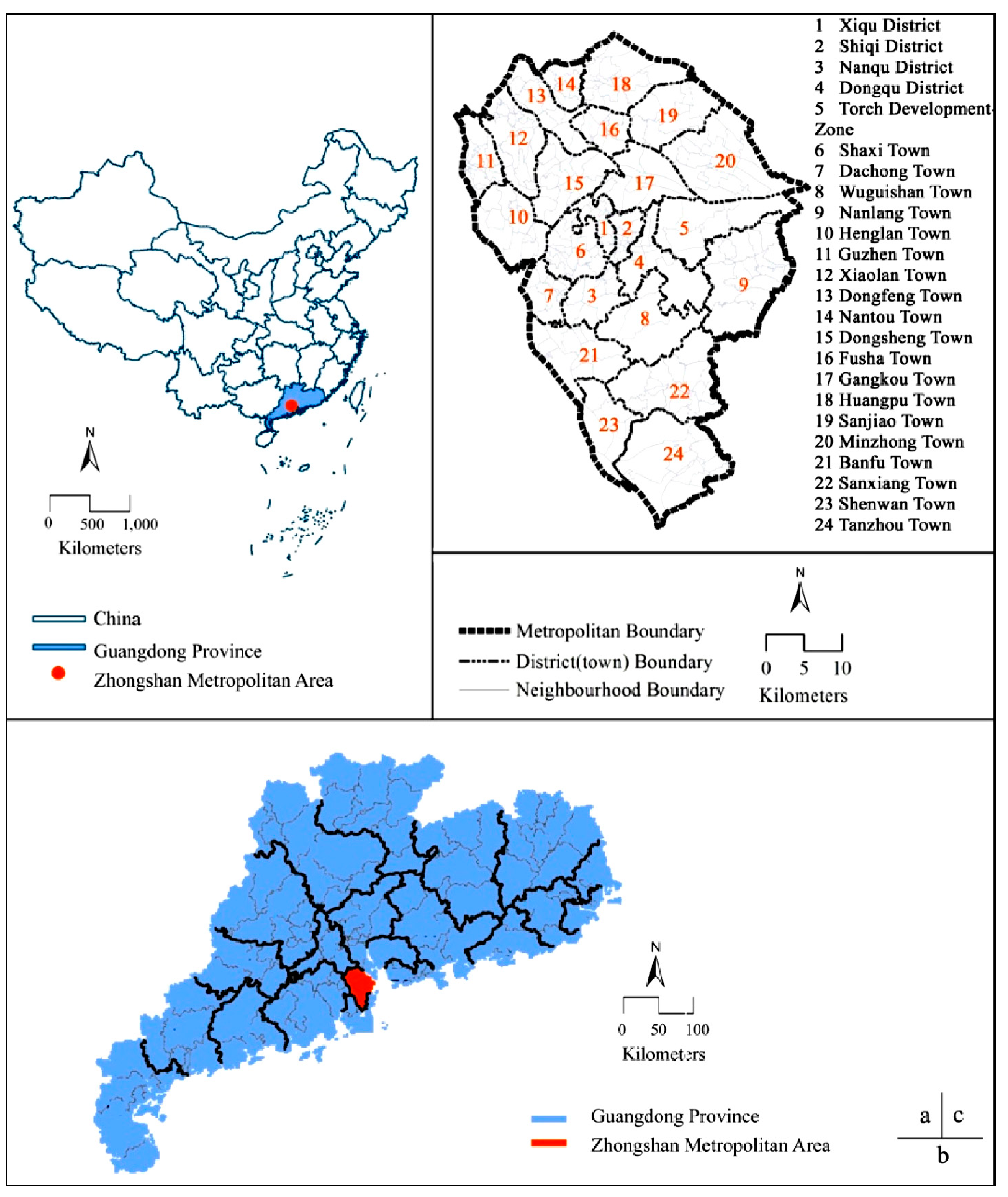
We chose the Zhongshan Metropolitan Area as our study area to examine the relationship between households’ motorized trips and the built environment in China’s medium-sized coastal cities with developed economies. Located in Guangdong Province of southern China and one of the three largest and most developed coastal urban agglomerations in China (
Figure 1), Zhongshan is a medium-sized prefecture-level city with an area of 1800 km
2 and a population of 3.1 million [
34]. The level of urbanization, income per capita, private car ownership per household and motorcycle ownership per household in Zhongshan (up to 2012) were 1.7-, 1.8-, 1.8- and 2.8-times of China’s average, respectively [
3,
35]. As of the time of research data collected in 2009, the type of transportation modes that were generally available in Zhongshan included walking, bicycle, electric bike, motorcycle, car, public transportation, school bus and company car. The modal split of car and motorcycle were 9.2% and 43.4%, respectively [
36], covering more than half of daily trips. The percentage of the primary industry, secondary industry and tertiary industry is 2.5%, 55.5% and 42%, respectively. The income per capita in year 2009 (as the year of research data collected) was 25,357 Chinese Yuan Renminbi (RMB) for urban residents and 14,928 RMB for rural residents. In China’s three largest coastal urban agglomerations, the Yangtze River Delta urban agglomerations, the Pearl River Delta urban agglomerations and the Jing-Jin-Ji urban agglomerations, there are nearly 20 medium-sized cities with similar levels of economic development, urbanization and motorization as Zhongshan. Generally, Zhongshan is representative as a medium-sized coastal city with its strong economy and high level of urbanization and motorization. In recent years, the rapidly increased vehicle use in cities like Zhongshan has led to severe urban traffic and environmental problems. To investigate the possible intervention of the built environment on growing vehicle use, it is imperative to conduct built environment/vehicle use-related studies in China.
3.2. Data Collection
In this study, we collected two types of data: built environment and household vehicle use. The built environment data were collected on the basis of traffic analysis zone (TAZ). TAZs are designed to be homogeneous with respect to socio-demographic characteristics, living conditions [
37] and, in most cases, share boundaries with administrative divisions. In some travel behavior/built environment studies, a neighborhood is spatially equivalent to a TAZ in this study. A total of 274 TAZs were included in this study. The built environment raw data include (
Table 2): (1) TAZ boundaries/proxy for neighborhood boundaries; (2) land use in 2010 with five major types of land use (residential land, commercial and service facilities, industrial and manufacturing, green space and other types of land uses); (3) population, dwelling units and employment in 2010; (4) street networks; (5) bus stops; and (6) political boundaries, such as city and town boundaries. The raw data of TAZ boundaries, city and town boundaries, street networks and bus stops were AutoCAD files, and we pre-processed them before importing them into ArcGIS.
The cross-sectional household vehicle use data include the household car trips and motorcycle trips. The data were derived from Zhongshan Household Travel Survey (ZHTS) in 2010 [
36]. ZHTS 2010 was conducted in the form of home interviews by the Zhongshan Planning Bureau. Selected by stratified random sampling covering the whole Zhongshan Metropolitan Area, the sample size was 30,000 households with a sample rate of 3.0%. The response rate was 85.4% of 25,618 households (excluding invalid data). The survey provided self-reported one-day travel diary data of all the members in a household, together with the personal and household socio-demographic data. We transformed the survey data in Microsoft Access, so that we could conduct further analysis in Stata.
Figure 1.
Study area.
(a) The location of Guangdong Province and Zhongshan Metropolitan Area in China; (b) the location of Zhongshan Metropolitan Area in Guangdong Province; and (c) the metropolitan boundary, district (town) boundary, neighborhood boundary and the location of all 24 districts (towns) in Zhongshan Metropolitan Area.
Table 2.
Raw data and sources. TAZ, traffic analysis zone.
Table 2.
Raw data and sources. TAZ, traffic analysis zone.
| Data | Sources |
|---|
| TAZ boundaries | Zhongshan Municipal Bureau of Urban Planning |
| Land use of each TAZ | Town-Level Bureau of Urban Planning |
| Population of each TAZ | Town-Level Bureau of Urban Planning |
| Dwelling units of each TAZ | Town-Level Bureau of Urban Planning |
| Employment of each TAZ | Town-Level Bureau of Urban Planning |
| Street networks | Zhongshan Municipal Bureau of Urban Planning |
| Bus stops | Zhongshan Municipal Bureau of Urban Planning |
| City and town boundaries | Zhongshan Municipal Bureau of Urban Planning |
| Household socio-demographic | Zhongshan Household Travel Survey |
| Household car and motorcycle trips | Zhongshan Household Travel Survey |
3.3. Characterization of Built Environment Attributes
Following previous studies, we identified ten built environment measures on the neighborhood level. Six measures (population density, dwelling unit density, employment density, street network density, intersection density and bus stop density,) are self-explanatory. What is worth mentioning, the streets included in the variable of street network density have at least one vehicle lane, due to the characteristics of the raw data of the street network. Furthermore, according to the raw data, a large part of these streets have pavements for walking, although the other part, mostly designed exclusively for vehicle use, does not.
Four other measures (bus service coverage rate, job accessibility, commercial accessibility and land use diversity) were calculated with respect to the context of Zhongshan or China, as applicable.
The bus service coverage rate, calculated by the ratio of bus service coverage to the total area of the neighborhood, reflects the level of bus services. In Chinese cities, the bus service area is defined as a the 300-meter radius of each bus station [
38].
The job accessibility is measured by the number of jobs accessible within ten minutes’ travel time from the centroid of a neighborhood during peak hours. The commercial accessibility is measured by the area coverage of commercial facilities within nine minutes’ travel time from the centroid of a neighborhood during peak hours. According to ZHTS, a ten-minute commute and a nine-minute shopping trip cover 70% of home-based work and home-based shopping, respectively; both are considered acceptable by commuters and shoppers.
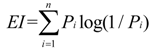
The land use diversity, calculated by the entropy index (EI) [
39], represents the degree to which different land uses in a neighborhood are mixed. EI is defined by:
where
n = number of unique land uses,
n ≥ 1;
Pi = percentage of land use and
i’s coverage over total land use coverage. A value of 0 indicates single-use environments, and 1 stands for the equalization of different land uses in area coverage. In China, the officially recommended proportion of residential land, industrial manufacturing land, commercial facilities land, green space land and other land is close to 2:2:1:1:1 [
40], which is applied in the land-use planning practice in Chinese cities, including Zhongshan. This proportion generates an entropy index of 0.67. Thus, each of the original entropy indices of a TAZ in this study is transformed into a criterion that is 0.67 of the standard 1, and all other indices are ranged between 0 and 1 based on the standard 1 [
41].
The ten measures are input data for factor analysis and cluster analysis thereafter to generate built environment factors and neighborhood types. Among the ten measures, population density, street network density, bus service coverage rate, job accessibility and land use mixture are chosen as the simple measures of a built environment representation and used in the models.
3.4. Classification of Neighborhood Types
Factor analysis and cluster analysis were combined to quantitatively classify neighborhood [
28]. Factor analysis was employed to remove the correlation and redundancy in the data and classify factors that capture different dimensions of built environment features [
28]. We obtained a set of five factors: density, street network design, destination accessibility, bus service accessibility and land use diversity, which were able to explain 91% of the total variation between the original ten measures altogether (
Table 3). More population, jobs and dwelling units in a neighborhood contributed to a higher loading of “density”. More street miles and intersections in a neighborhood yielded a higher loading of “street design”. More jobs and commercial facilities within a certain travel time contributed to a higher loading of “destination accessibility”. More bus stops and better bus-service resulted in a higher loading of “bus service accessibility”. A neighborhood with more mixed land-use development tended to load heavier on “diversity”.
Table 3.
Factor analysis of each built environment dimension.
Table 3.
Factor analysis of each built environment dimension.
| Measures | Factor 1 | Factor 2 | Factor 3 | Factor 4 | Factor 5 |
|---|
| Density | Street network design | Destination accessibility | Bus service accessibility | Land use diversity |
|---|
| Employment density | 0.9504 | 0.0078 | −0.1450 | 0.1136 | 0.1014 |
| Dwelling unit density | 0.8040 | 0.0958 | 0.1582 | −0.0162 | −0.0548 |
| Population density | 0.7785 | 0.1631 | 0.1363 | −0.0378 | −0.0743 |
| Intersection density | 0.1070 | 0.9782 | −0.0730 | −0.0452 | −0.0004 |
| Street network density | 0.0660 | 0.8292 | 0.0859 | 0.0801 | 0.0293 |
| Commercial accessibility | 0.0235 | −0.0122 | 0.9648 | −0.0136 | 0.0542 |
| Job accessibility | 0.2552 | 0.1045 | 0.5109 | 0.1992 | −0.0213 |
| Bus station density | 0.1484 | −0.0611 | −0.1060 | 0.9538 | 0.0147 |
| Bus service coverage rate | −0.1163 | 0.0969 | 0.1894 | 0.8179 | −0.0319 |
| Land use mixture | −0.0034 | 0.0125 | 0.0443 | −0.0077 | 0.9908 |
| % Variation | 24% | 22% | 21% | 19% | 5% |
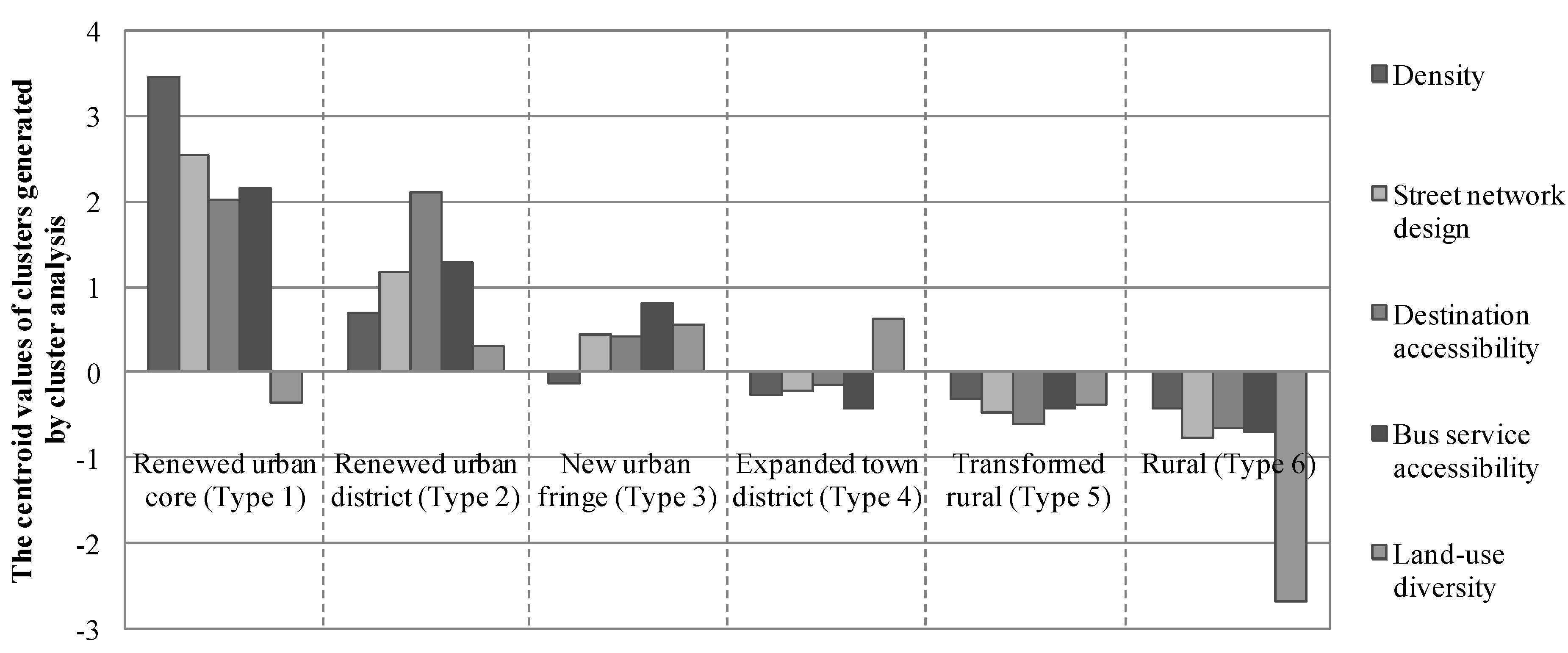
Cluster analysis was then used to examine and distinguish the variation in the built environment among the 274 neighborhoods on the basis of the five factors. This study used a K-means cluster analysis to partition neighborhoods into the nearest cluster with the nearest mean considering similarities and dissimilarities in the values of the factors. The nearest cluster had the smallest Euclidean distance between the observation and the centroid of the cluster. After an iterative and heuristic process [
27], we finally determined six clusters (
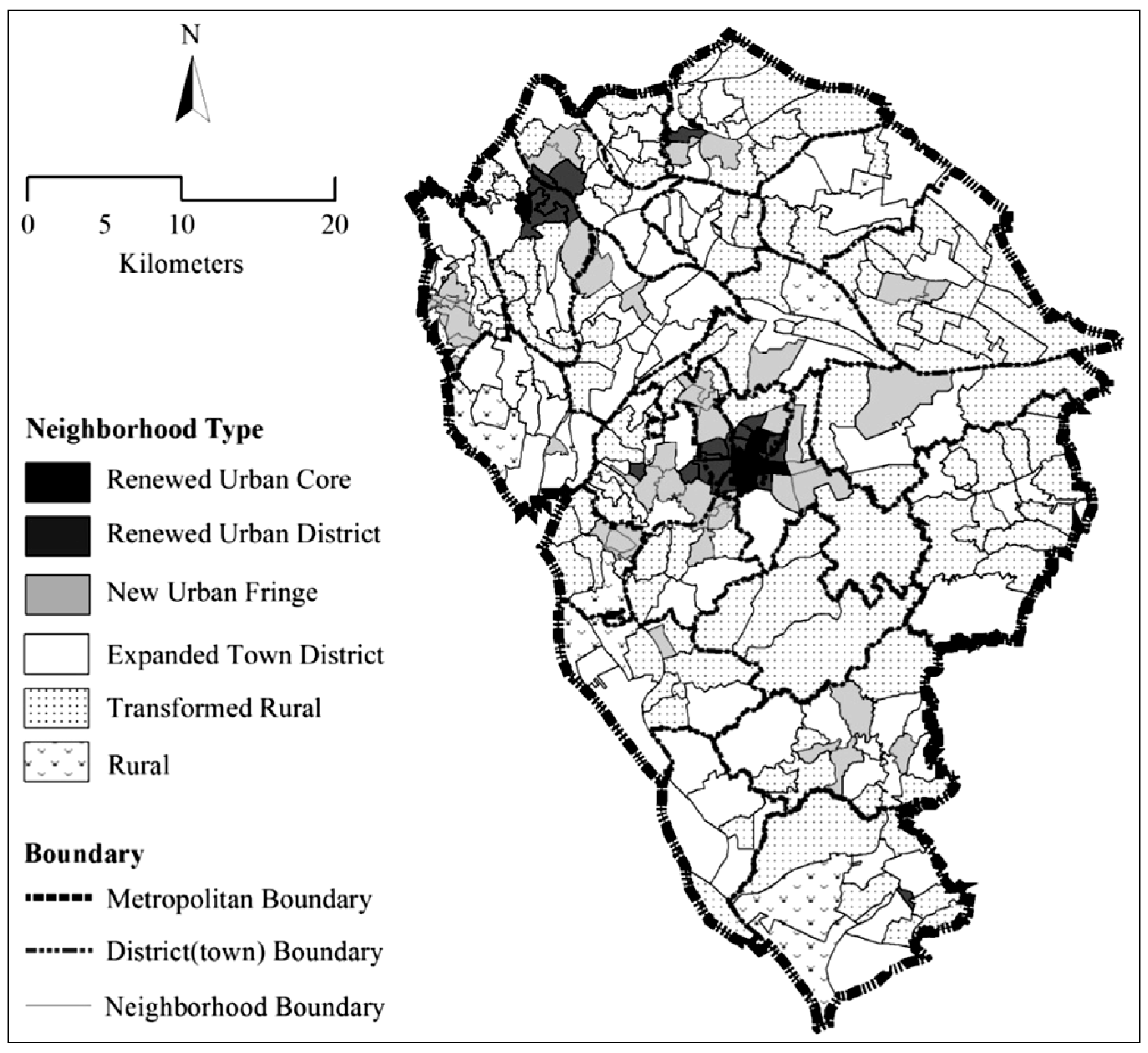
Figure 2) as neighborhood types to best categorize all neighborhoods in Zhongshan. The centroid values of each reflected the distinctive built environment features. Considering the built environment features and geographical location, the six neighborhood types were named as renewed urban core, renewed urban district, new urban fringe, expanded town district, transformed rural and rural neighborhoods (
Figure 3).
3.5. Model Specification
Because the household car and motorcycle trips are non-negative, count-dependent variables, we tested the data to choose the proper models. Due to the characteristics of the dependent variables (
Table 4), we preferred negative binomial regression (NBR) to Poisson regression, as many similar studies have done [
42,
43]. Then, the results of the Vuong model selection test strongly favored a standard NBR over a zero-inflated NBR.
Figure 2.
Centroid values of each neighborhood type.
Figure 2.
Centroid values of each neighborhood type.
Figure 3.
Location of Zhongshan’s neighborhoods by type.
Figure 3.
Location of Zhongshan’s neighborhoods by type.
A negative binomial regression model linking household motorized trips to the built environment is defined (for similar formulations, see [
43]). We employed the same independent variable sets in household car trips models and motorcycle trips models. The model specifications for the basic models were expressed as follow:
where HHSIZE is the household size (aged over 5); EMPLOYED stands for the number of employment; STUDENT is the number of students in primary and high schools; HOUSE denotes the house ownership; HIGHINC and MEDINC are dummies for the annual income ranges of above 60,000 RMB and 20,000–60,000 RMB (with a reference category of under 20,000 RMB as low income, LOWINC); BUSDIST demonstrates the distance of the nearest bus stop from home; BIKES, EBIKES, MOTORS and CARS represent the number of bicycles, electric-bikes, motorcycles and cars, respectively.
Along with the basic model, the regression of the dependent variables proceeded in two expanded models. The expanded Model 1 adds five simple built environment measures of the neighborhood where the household is located as independent variables, in which POPDEN, STDEN, JOBACC, BUSSERV and LANDDIV demonstrate the population density, street network density, job accessibility, bus service coverage rate and land-use mixture. The expanded Model 2 was estimated, where the simple measures are replaced by the neighborhood types. The choice of neighborhood is represented by five neighborhood types, renewed urban core (RENEW_CORE), renewed urban district (RENEW_URBAN), new urban fringe (NEW_FRINGE), expanded town district (EXPD_TOWN) and transformed rural (TRANS_RURAL), each a dummy with its own coefficient; rural neighborhoods (RURAL) serve as the reference category.
5. Discussion and Policy Implications
This paper presented findings from a study aimed at exploring the relationship of the built environment and household vehicle use in the Chinese context. With data collected from 274 neighborhoods in the Zhongshan Metropolitan Area, we first characterized ten neighborhood-level built environment measures and chose five out of the ten as independent variables, which capture different built environment features. We then employed factor and cluster analysis to classify neighborhoods in Zhongshan into six types based on the ten measures. Finally, we examined specifically how the built environment in Zhongshan serves to illuminate the household car and motorcycle trips with negative binomial models.
The household socio-demographic measures, i.e., the income level, household composition and the availability of vehicles, show significant association with car and motorcycle use, conforming to expectation. To be specific, having more household members employed or as students or owning cars or motorcycles are factors highly related to more frequent vehicle use. An increasing ownership of bikes or electric-bikes or adjacency to the nearest bus stop, however, are found to be substantially associated with less household car or motorcycle trips. The findings imply that with the improvement of overall living standards and growing ownership of vehicles, households in Zhongshan are very likely to generate more vehicle use.
With regard to the correlations of the built environment, we found out that adding built environment variables in the form of simple measures or neighborhood types enhances the explanatory powers of the models, albeit to varying degrees. As the elasticities have revealed (
Table 7), the street network density played a significantly positive role in both household car and motorcycle trips. Compared to the households in the neighborhoods with less connective street networks, the households in the neighborhoods with highly connected and denser street networks would generate more car and motorcycle trips. For example, if the street network density doubled from the average value of 3.10 (
Table 4) to 6.20 (km/km
2), a household’s car and motorcycle trips would, all else being equal, increase by 0.15 trips and 0.44 trips, respectively. The population density plays a negative role in vehicle use in Zhongshan. That implies households in the more populated environments may generate fewer car or motorcycle trips than in the less populated environments. The reason for this relationship, we hypothesize, is because the compact urban form, closely related to high population density, increases the possibility of having short-to-medium distance trips instead of long-distance ones [
41]. The job accessibility is only significant for car trips and the bus service coverage rate for motorcycle trips. The findings indicate that, all else being equal, more accessible jobs are related to less car use. Furthermore, with convenient public transportation services, a household may generate less motorcycle trips. Interestingly, the measure of land use diversity is insignificantly related to vehicle use in Zhongshan, inconsistent with some research findings in the Western context [
39]. In this study, the mean land use diversity of Zhongshan is as high as 0.69. On the contrary, in Western studies in which land use diversity was significantly related to travel behavior, the mean land-use diversity ranged only from 0.29 to 0.48 [
16,
46,
47], much lower than that of Zhongshan. Therefore, we assumed that in areas already with very mixed land use development, e.g., Zhongshan Metropolitan Area, the effect of land-use diversity on motorized trips may be very limited. However, further study is needed with specifically collected data.
Currently, in Zhongshan and many other Chinese cities, urbanization features highly dense land use development, improvement of street networks for cars and motorcycles and, yet, slow development of the transit system. As the compact urban form involving dense land use development is related to less car and motorcycle use, the construction of street networks and insufficient concentration on the transit system may be associated with an increase of car and motorcycle use. To potentially reduce car and motorcycle use, it may be informative to form land use developments with a relatively high population density, slow down the construction of street networks, provide more jobs adjacent to residential areas and facilitate easy access to public transportation services. Those may provide planners and policy makers with insights into suitable policies and measures to control car and motorcycle use and promote sustainable transportation.
6. Strengths and Limitations
This study has a number of strengths and limitations. In terms of the strengths, the study investigated two built environment representations in the Chinese context, simple built environment measures and neighborhood types, with a quantitative approach. That would facilitate the emerging built environment/travel behavior research in China. Secondly, the study focused on fast-growing vehicle use and provided informative policy implications for policy makers. Finally, the study revealed the effects of the built environments on vehicle use in the context of rapid urbanization and motorization, potentially promoting further the comparative research between different contexts.
In terms of the limitations, the study was restricted to a single geographical area, the Zhongshan Metropolitan Area. The results, therefore, may not be generalizable to other geographical characteristics that are different from Zhongshan. Moreover, cross-sectional data were used in this study. The full evaluation of causal inferences about built environment effects on car and motorcycle use will require longitudinal and multilevel analyses over time. Finally, the characteristics of vehicle trips, e.g., travel purpose, trip time and travel cost, were not incorporated in the study due to the limited data.
7. Conclusions
This study adds to the existing literature by exploring the relationship between two built environment representations and household vehicle use in the Chinese context with data collected in Zhongshan Metropolitan Area. First, ten built environment measures were characterized and five among them were chosen as independent variables, which capture five built environment features. Then, factor and cluster analyses were performed to classify neighborhoods in Zhongshan into six types based on the ten measures. Finally, negative binomial models were used to examine specifically how household car and motorcycle trips related to the built environment measures and neighborhood types. The results suggest that household measures show significant association, and built environment variables enhance the explanatory powers of the models, albeit to varied degrees. All else being equal, street network density is positively associated with more household vehicle use, while population density is negative. The job accessibility is negatively related to car use and the bus service to motorcycle use.
In order to reduce car and motorcycle use, this paper enlightens planners and policy makers in Zhongshan to form a relatively high density of land-use developments, slow down the construction of street networks, provide more jobs adjacent to residential areas and facilitate easy access to public transportation services. This study is one of very few to incorporate the built environment into a travel behavior-related study. It facilitates the understanding of the relationship between the built environment and household car and motorcycle use in the Chinese context, which provides insights for urban planners, transportation planners and policy makers.
Future studies in this field could be improved by: (1) testing the influence of the built environment on the individual’s mode choice; (2) incorporating the built environment features of trip destinations into the models; (3) presenting travel time, travel cost and self-selection factors into the study and testing their influence on travel behavior [
18,
48,
49]; and (4) conducting a comparative study across a set of representative Chinese cities to reinforce external validity in the Chinese context.


