Influence of the Thermal Inertia in the European Simplified Procedures for the Assessment of Buildings’ Energy Performance

Abstract

This study aims to highlight the importance of thermal inertia in buildings. Nowadays, it is possible to use energy analysis software to simulate the building energy performance. Considering Italian standards, these analyses are based on the UNI TS 11300 that defines the procedures for the national implementation of the UNI EN ISO 13790. These standards require an energy analysis under steady-state condition, underestimating the thermal inertia of the building. In order to understand the inertial behavior of walls, a cubic Test-Cell was modelled through the dynamic calculation code TRNSYS and three different wall types were tested. Different stratigraphies, characterized by the same thermal transmittance value, composed by massive elements and insulating layers in different order, were simulated. Through TRNSYS, it was possible to define maximum surface temperatures and to calculate thermal lag between maximum values, both external and internal. Moreover, the attenuation between external surface temperatures and internal ones during summer (July) was calculated. Finally, the comparison between Test-Cell’s annual energy demands, performed by using a commercial code based on the Italian standard UNITS 11300 and the dynamic code, TRNSYS, was carried out.

1. Introduction

Improving thermal performance of buildings is the first step to reduce annual energy demand and, consequently, air pollution. In fact, through the Directive 2002/91/CE the European Community highlighted how the increase of energy efficiency is a point of strength within the set of measures and actions necessary to comply with the Kyoto Protocol [1]. Regarding building envelope, the first intervention is related to the thermal transmittance value reduction but it is important to emphasize the building energy savings that could be achieved by exploiting thermal inertia. Buildings’ massive walls store heat when the heating plant is working and, during the summer, they contribute to the phase shift of the external thermal waves. The theoretical approach to this problem is related to the inertial properties of a wall, an issue that dates back to the classical work by Fourier dealing with transient heat conduction in a system, modeled by a semi-infinite wall—consisting of a homogeneous, isotropic medium—to which a sinusoidal temperature fluctuation is applied. Currently, the thermal inertia evaluation is done using numerical methods and several authors evaluated the influence of the walls thermal properties on the building energy performance, by comparing different construction systems [2,3,4,5,6]. Kossecka and Kosny report numerical simulations that lead to the conclusion that the material configuration of the exterior wall can significantly affect the annual energy demand of the whole building; however, this effect depends on the type of climate [7]. In order to correctly evaluate buildings inertial properties it is important to employ models that take into account all thermal characteristics likethermal conductivity, mass density and, obviously, specific heat capacity. In the case study by De LietoVollaro et al. [8] a dynamic software is used to evaluate the energy demand of a historical building and thermal inertia is taken into account by means of the advanced calculation code TRNSYS. Ferrari and Baldinazzo [9] analyzed buildings behavior considering the Italian standard (UNITS 11300 [10]) and they concluded that thermal capacity has a minor role in simplified procedures. These standards require an energy analysis under semi-stationary conditions, considering monthly temperatures and monthly solar radiation values. Asdrubali et al. [11] also made a comparison between Italian and Spanish national regulations, analyzing three typical buildings and evaluating the contribution to total energy demand in winter and summer conditions. The Italian standard UNI TS 11300 defines the procedures for the national implementation of the UNI EN ISO 13790 [12]. Regarding the evaluation of the inertial behavior, the determination of the utilization factors and thermal lag refers to the UNI EN ISO 13786 [13]. In cases where the building’s stratigraphy is not available (e.g., existing buildings), the thermal capacity per unit area of envelope is provided by tabulated data. The heating and cooling energy balance equations reported in the UNI TS 11300 are given as follows:

Q_H,nd = (Q_H,tr + Q_H,ve) − η_H,gn (Q_int + Q_sol)

(1)

Q_C,nd = (Q_int + Q_sol) − η_C,Is (Q_C,tr + Q_C,ve)

(2)

where Q_H,nd and Q_C,nd represent the energy demands for heating and cooling, respectively, Q_H,tr represents the heat dissipation through opaque and transparent surfaces, Q_H,ve represents ventilation losses, Q_int represents the internal gains and Q_sol represents the solar gains. Building’s dynamic parameters are included into utilization factors: a utilization factor of thermal contributions η_H,gn and a utilization factor of thermal dispersion η_C,Is. The thermal energy stored by a massive wall is not explicitly included in Equations (1) and (2), but is taken into account through the coefficients η_H,gn and η_C,Is. Considering the heating demand, the heat gain and loss ratio γ_H is defined as follows:

(3)

where Q_gn = Q_int + Q_sol and Q_H,ht = Q_H,tr + Q_H,ve. The utilization factor η_H,gn is defined in the standard as

(4)

(5)

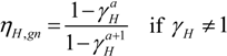
where a is a parameter depending on the time constant τ.

(6)

(7)

C is the internal heat capacity of a building, H is the total heat loss coefficient of the building caused by transmission and ventilation heat losses. In equation (7), a₀ is a numerical parameter and τ₀ is a reference time constant. For cooling needs η_C,Is is defined in a similar fashion.

2. Modeling

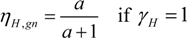
In this study three walls were modelled by TRNSYS software [14]. This software is based on a dynamic model that allows to appreciate the variation of physical phenomena, overcoming the limitations related to semi-stationary methods. TRNSYS allows to take into account the variation of external temperature and solar radiation and it is based on a calculation code that applies the transfer function relationships developed by Mitalas [15]. This software is composed of two parts: TRNSYS-Build that allows the user to generate the model and TRNSYS-Studio, used to apply the external environmental conditions. The used weather-data have been recorded at Rome-Fiumicino. The walls were analyzed considering the first day of July and south facing. Each wall consists of two base materials (see Table 1): heavy concrete and extruded polystyrene, XPS in the following. As shown in Table 2, Wall 1 is characterized by a massive layer located at the inner side of the wall. Wall 2 is characterized by the XPS layer on the center. Finally, Wall 3 has the XPS layer on the outer face and the heavy concrete inside. All the walls share the same thermal transmittance value but the different layers order involves a different wall behavior in terms of thermal inertia. Figure 1 shows walls schemes.

Table 1. Material’s properties.

Material	Thermal Conductivity [W/m K]	Specific Heat Capacity [kJ/kg K]	Mass Density [kg/m3]
Heavy Concrete	1.700	0.84	2200
XPS	0.034	1.45	33.5

Table 1. Material’s properties.

Material	Thermal Conductivity [W/m K]	Specific Heat Capacity [kJ/kg K]	Mass Density [kg/m3]
Heavy Concrete	1.700	0.84	2200
XPS	0.034	1.45	33.5

Table 2. Walls’ stratigraphy.

−		Wall 2		Wall 3
	Thickness [m]		Thickness [m]		Thickness [m]
Ext	−	Ext	−	Ext	−
Heavy Concrete	0.2	Heavy Concrete	0.1	XPS	0.02
XPS	0.02	XPS	0.02	Heavy Concrete	0.2
		Heavy Concrete	0.1
Int	−	Int	−	Int	−
U-Value [W/m2 K]	1.139	U-Value [W/m2 K]	1.139	U-Value [W/m2 K]	1.139
Solar Absorbance	0.6	Solar Absorbance	0.6	Solar Absorbance	0.6

Table 2. Walls’ stratigraphy.

−		Wall 2		Wall 3
	Thickness [m]		Thickness [m]		Thickness [m]
Ext	−	Ext	−	Ext	−
Heavy Concrete	0.2	Heavy Concrete	0.1	XPS	0.02
XPS	0.02	XPS	0.02	Heavy Concrete	0.2
		Heavy Concrete	0.1
Int	−	Int	−	Int	−
U-Value [W/m2 K]	1.139	U-Value [W/m2 K]	1.139	U-Value [W/m2 K]	1.139
Solar Absorbance	0.6	Solar Absorbance	0.6	Solar Absorbance	0.6

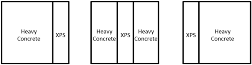
Figure 1. Walls’ stratigraphy.

Figure 1. Walls’ stratigraphy.

In order to perform a simple simulation, a small building model was created. This simple model is a cubic test-cell characterized by a direct contact with the ground. The six faces of the cell are equal in terms of stratigraphy and there are no windows. Each wall has a surface of 5 m × 5 m. No shading system, internal gain nor air renovation rate were considered.

The test cell is resting on the ground and the floor was considered as an adiabatic surface. The floor and the ceiling are characterized by the same walls’ stratigraphy.

As shown in Figure 2, each face of the cell has a different exposure, corresponding to North, East, South and West, respectively.

Figure 2. Test-cell exposure.

Figure 2. Test-cell exposure.

3. Results and Discussion

TRNSYS software is a tool that allows to calculate time-dependent internal and external surface temperatures using a selected time-step, set to 1 h in our simulations. Through this tool, it is possible to evaluate wall’s thermal inertia and, consequently, calculate surface’s thermal attenuation and thermal lag between interior and exterior faces. As already said, the weather-data used refers to Rome-Fiumicino. The walls were analyzed considering the first day of July and south facing.

The surface temperature fluctuations of Wall 1, the ambient temperature and the internal temperature are shown in Figure 3.

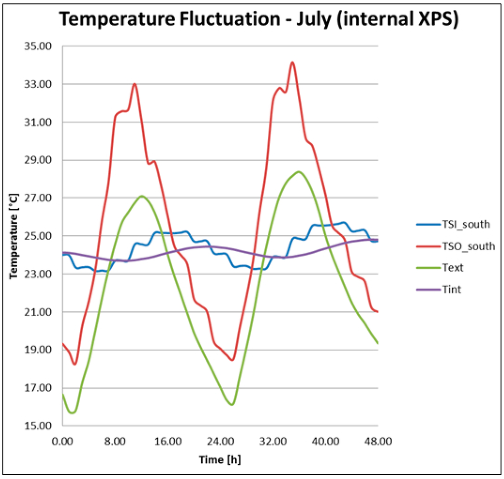
Figure 3. Wall 1 temperature fluctuations.

Figure 3. Wall 1 temperature fluctuations.

Analyzing the first 24 h, Table 3 shows the highest surface temperature values, the temperature difference between surfaces and the thermal lag.

Table 3. Wall 1 temperature variation and thermal lag.

Wall 1	Maximum External Surface Temperature [°C]	Maximum Internal Surface Temperature [°C]	Surface Temperature Variation (Ext-Int) [°C]	Thermal Lag [h]
	33.01	25.21	7.80	7

Table 3. Wall 1 temperature variation and thermal lag.

Wall 1	Maximum External Surface Temperature [°C]	Maximum Internal Surface Temperature [°C]	Surface Temperature Variation (Ext-Int) [°C]	Thermal Lag [h]
	33.01	25.21	7.80	7

Similarly for Wall 2 and Wall 3, Figure 4 and Figure 5 and Table 4 and Table 5 show the respective temperature fluctuation and their thermal lag.

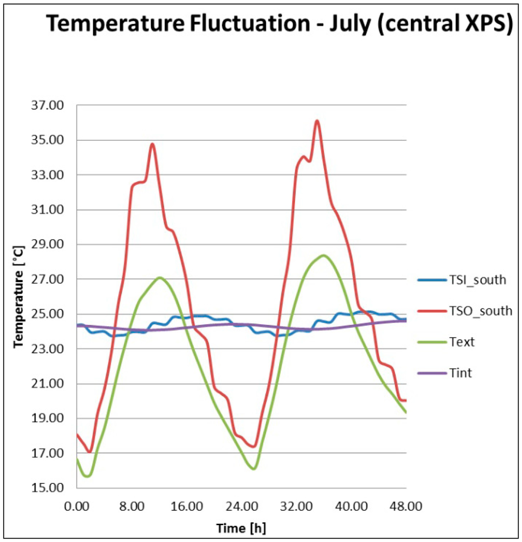
Figure 4. Wall 2 temperature fluctuations.

Figure 4. Wall 2 temperature fluctuations.

Table 4. Wall 2 temperature variation and thermal lag.

Wall 2	Maximum External Surface Temperature [°C]	Maximum Internal Surface Temperature [°C]	Surface Temperature Variation (Ext-Int) [°C]	Thermal Lag [h]
	34.78	24.89	9.90	6

Table 4. Wall 2 temperature variation and thermal lag.

Wall 2	Maximum External Surface Temperature [°C]	Maximum Internal Surface Temperature [°C]	Surface Temperature Variation (Ext-Int) [°C]	Thermal Lag [h]
	34.78	24.89	9.90	6

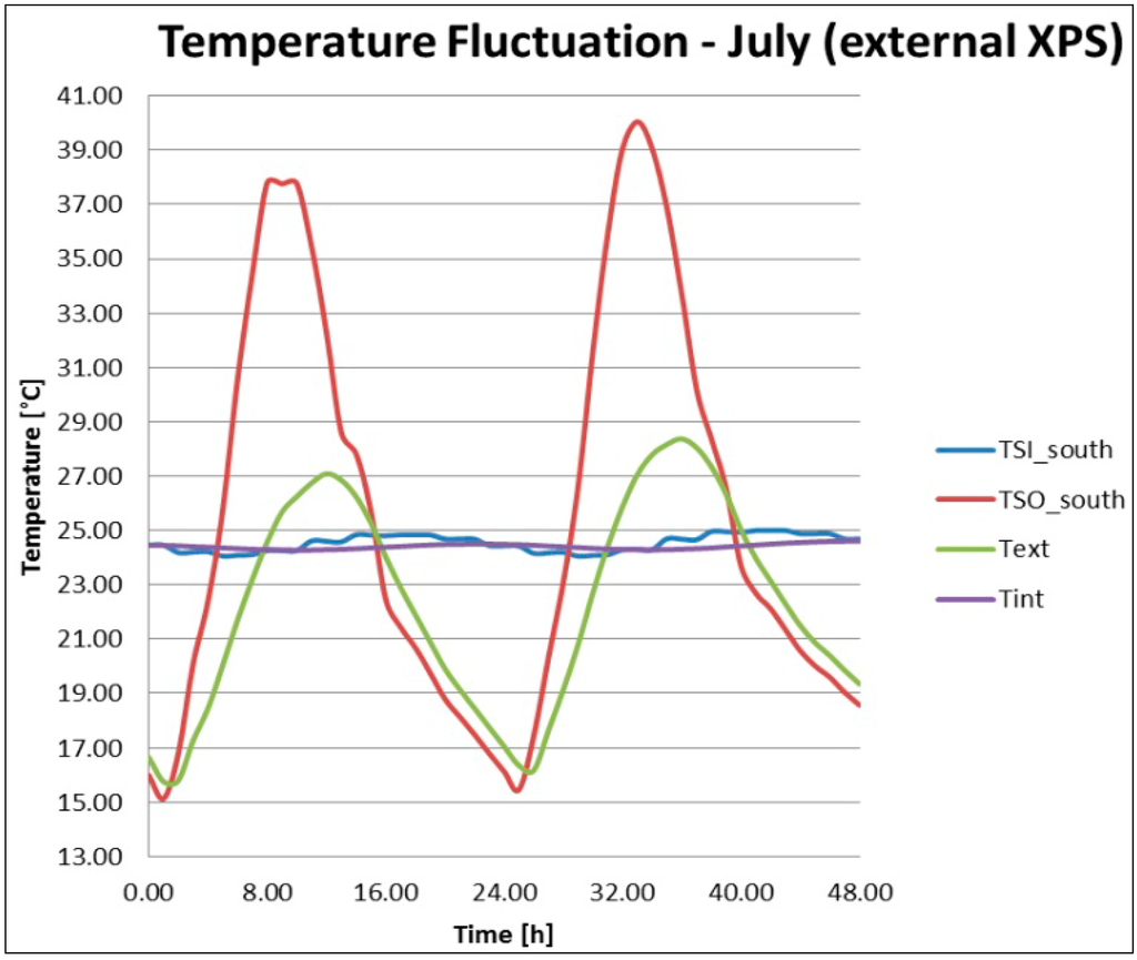
Figure 5. Wall 3 temperature fluctuations.

Figure 5. Wall 3 temperature fluctuations.

Table 5. Wall 3 temperature variation and thermal lag.

Wall 3	Maximum External Surface Temperature [°C]	Maximum Internal Surface Temperature [°C]	Surface Temperature Variation (Ext-Int) [°C]	Thermal Lag [h]
	37.81	24.85	12.96	9

Table 5. Wall 3 temperature variation and thermal lag.

Wall 3	Maximum External Surface Temperature [°C]	Maximum Internal Surface Temperature [°C]	Surface Temperature Variation (Ext-Int) [°C]	Thermal Lag [h]
	37.81	24.85	12.96	9

Wall 3 presents the highest external surface temperature value but, at the same time, the internal surface temperature is the lowest, with a difference of 12.96 °C and a thermal lag of 9 h. Wall 1 and Wall 2 present thermal lags and surface temperature variations lower than Wall 3. Observing Figure 3, Figure 4 and Figure 5, it is possible to notice a progressive reduction of the internal temperature oscillation amplitude. This indicates the dynamic software capability to consider the transient behavior of the building masses.

To understand the inertial behavior of these walls, the internal air temperature of the Test-Cell was plotted during June, July, August and September, with the cooling system not running. The air temperature variation and the hypothetic air-conditioning set-point value equal to 26 °C are shown in Figure 6.

Figure 6 allows to evaluate the temperature derivative and it is possible to observe how Wall 3 always has the lower slope.

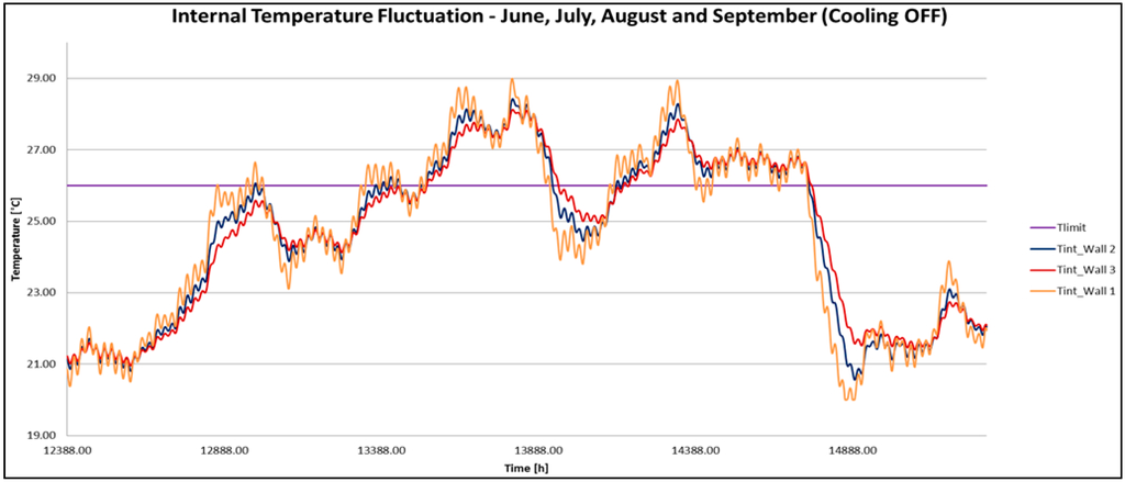
Figure 6. Test-Cell internal air temperature fluctuations from June to September.

Figure 6. Test-Cell internal air temperature fluctuations from June to September.

As mentioned, these three wall types were reproduced in a Test-Cell using TRNSYS and, for the sake of comparison, with a commercial software used for buildings certification. This final step is important to understand to what extent simplified procedures are able to take into account materials properties as specific heat capacity and mass density. Table 6 shows thermal lag values and attenuation factors calculated by means of the formulas reported in the UNI EN ISO 13786. It is possible to observe that there is a difference between thermal lag evaluated through the European standard and the same calculated with TRNSYS (Table 3, Table 4 and Table 5).

Table 7 shows the comparison between the calculated energy demands, highlighting the percentage differences.

Table 6. Thermal lag and attenuation factor calculated through the UNI EN ISO 13786.

UNI EN ISO 13786	Thermal Lag [h]	Attenuation Factor
Wall 1	5.7	0.451
Wall 2	7.2	0.418
Wall 3	6.7	0.266

Table 6. Thermal lag and attenuation factor calculated through the UNI EN ISO 13786.

UNI EN ISO 13786	Thermal Lag [h]	Attenuation Factor
Wall 1	5.7	0.451
Wall 2	7.2	0.418
Wall 3	6.7	0.266

Table 7. Annual energy demands and percentage differences.

Wall type	QH,nd TRNSYS [kWh]	QH,nd UNI TS 11300 [kWh]	Heating Percentage Difference [%]	QC,nd TRNSYS [kWh]	QC,nd UNI TS 11300 [kWh]	Cooling Percentage Difference [%]
Wall 1	4837.63	5115.19	−5.43	170.49	607.78	−71.95
Wall 2	4802.31	5117.70	−6.16	148.22	608.43	−77.09
Wall 3	4771.66	5142.67	−7.21	140.02	611.71	−77.11

Table 7. Annual energy demands and percentage differences.

Wall type	QH,nd TRNSYS [kWh]	QH,nd UNI TS 11300 [kWh]	Heating Percentage Difference [%]	QC,nd TRNSYS [kWh]	QC,nd UNI TS 11300 [kWh]	Cooling Percentage Difference [%]
Wall 1	4837.63	5115.19	−5.43	170.49	607.78	−71.95
Wall 2	4802.31	5117.70	−6.16	148.22	608.43	−77.09
Wall 3	4771.66	5142.67	−7.21	140.02	611.71	−77.11

Figure 7 and Figure 8 show the differences between energy demands calculated through the two software.

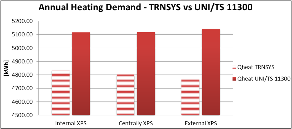
Figure 7. Annual heating demand comparison.

Figure 7. Annual heating demand comparison.

Figure 8. Annual cooling demand comparison.

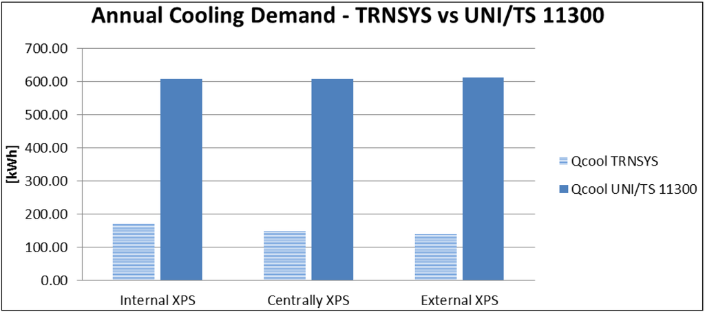
Figure 8. Annual cooling demand comparison.

As shown by TRNSYS simulations, Wall 3—with the XPS layer positioned at the outside face—represents the best configuration. This wall is characterized by the highest difference between internal and external surface temperature. Indeed, TRNSYS annual heating demand is the lowest. Comparing energy demand for heating, it is possible to observe that TRNSYS has lower values than the commercial software. Furthermore, the commercial software would indicate that Wall 3 is the lowest performing, differently from what found by TRNSYS simulations. On the contrary, analysing the energy demand for cooling, TRNSYS values are much lower than the ones calculated by the commercial software.

The simulations performed using the stationary software have provided results with no significant variations. Considering Wall 3, the thermal lag calculated through the commercial tool (and therefore following the European standard) is different from the corresponding value calculated with TRNSYS; moreover, the attenuation factor is lower, but the heating and cooling demands are always higher. This suggests that simplified procedures, applying the UNI EN ISO 13786 to calculate the dynamic parameters, are not able to take into account the actual building’s thermal inertia. The reduction of the attenuation factor from 0.451 to 0.266 for the three wall types implies the progressive growth of the walls thermal storage ability and a resulting energy demands reduction, both in winter and summer. Stationary software outputs, shown in Table 7, do not provide satisfactory design indications because the best solution has been considered as the worst. Moreover, it is possible to observe a reduced spread of the results compared with what obtained by TRNSYS. Indeed, considering the cooling demand, the lower values are due to the building heat disposing during night hours. Analyzing the heating demand, the lower values are due to the wall’s heat storage when the heating plant is on.

4. Conclusions

Three wall types were analyzed by using the dynamic software TRNSYS. The differences between these walls consist in a different stratigraphy—massive elements and an insulating layer in a different order—but the same thermal transmittance. The south face of a cubic Test-Cell was simulated and its internal and external surface temperatures were calculated through the dynamic tool.

The Test-Cell internal air temperature was plotted from June to September, considering the cooling system not running and, finally, annual energy demands were calculated by using TRNSYS and, for comparison, by a commercial software based on the standard UNI TS 11300. Analyzing internal and external surface temperatures, attenuation factors and thermal lags, it is possible to conclude that Wall 3 represents the best configuration to mitigate environmental conditions. Wall 3 stratigraphy allows us to obtain the lowest internal surface temperatures, with the highest thermal lag. Testing Wall 3 by using TRNSYS and the stationary software, it is possible to observe that the stationary code has not provided the same result as the dynamic one. Indeed, in the steady-state software the wall’s stratigraphy and therefore the position of the insulating layer do not have an effective role. Using a simplified procedure, it is impossible to appreciate the actual effect of the massive layers’ position on annual energy demands. For this reason, these procedures do not allow to correctly evaluate the buildings’ inertial behaviour and their energy performance. Current regulations impose severe restrictions on consumption. Consequently, the energy saving issue is more relevant than ever and the irresponsible use of resources is a luxury we cannot afford. The 2020 climate and energy package is the first deadline to improve the buildings energy efficiency, but we need more efficient simulation tools. To achieve this goal, it is absolutely necessary to review the design of buildings and plants and make them more efficient, especially in a country like Italy, where the energy demand in the building sector covers a market share of around 41% of national energy consumption.

References and Notes

- European Parliament. European Directive 2002/91/CE on the energy performance of buildings. Available online: http://eur-lex.europa.eu/legal-content/EN/TXT/?uri=CELEX:32002L0091 (accessed on 5 June 2014).
- Gregory, K.; Moghtaderi, B.; Sugo, H.; Page, A. Effect of thermal mass on the thermal performance of various Australian residential construction systems. Energy Build. 2008, 40, 459–465. [Google Scholar] [CrossRef]
- Collet, F.; Serres, L.; Miriel, J.; Bart, M. Study of thermal behavior of clay wall facing south. Build. Environ. 2006, 41, 307–315. [Google Scholar] [CrossRef]
- Bojic, M.; Yik, F.; Sat, P. Influence of thermal insulation position in building envelope on the space cooling of high-rise residential building in Hong Kong. Energy Build. 2001, 33, 569–581. [Google Scholar] [CrossRef]
- Aste, N.; Angelotti, A.; Buzzetti, M. The influence of the external walls thermal inertia on the energy performance of well insulated buildings. Energy Build. 2009, 41, 1181–1187. [Google Scholar] [CrossRef]
- Bond, D.E.M.; Clark, W.W.; Kimber, M. Configuring wall layers for improved insulation performance. Appl. Energy 2013, 112, 235–245. [Google Scholar] [CrossRef]
- Kossecka, E.; Kosny, J. Influence of insulation configuration on heating and cooling loads in a continuously used building. Energy Build. 2002, 34, 321–331. [Google Scholar] [CrossRef]
- De LietoVollaro, R.; Evangelisti, L.; Carnielo, E.; Basilicata, C.; Battista, G.; Gori, P.; Guattari, C.; Fanchiotti, A. An Integrated Approach for an Historical Buildings Energy Analysis in a Smart Cities Perspective. Energy Procedia 2014, 45, 372–378. [Google Scholar] [CrossRef]
- Ferrari, S.; Baldinazzo, M. Assessment of the energy performance of buildings: From simplifiedprocedures to dynamicanalysis. In Proceedings of the AICARR Conference, Certificazione energetica: Normative e modelli di calcolo per il sistema edificio-impianto posti a confronto.
- UNI TS 11300-1, Determination of the buildingsenergydemand for the air-conditioning in summer and winter. (In Italian: Determinazione del fabbisogno di energia termica dell’edificio per la climatizzazione estiva ed invernale.)
- Asdrubali, F.; Bonaut, M.; Battisti, M.; Venegas, M. Comparative study of energy regulations for buildings in Italy and Spain. Energy Build. 2008, 40, 1805–1815. [Google Scholar] [CrossRef]
- UNI EN ISO 13790, Energy performance of buildings—Calculation of energy use for heating and cooling.
- UNI EN ISO 13786, Thermal performance of building components—Dynamic thermal characteristics—Calculation methods.
- Transient System Simulation Tool. Available online: http://sel.me.wisc.edu/trnsys (accessed on 5 June 2014).
- Mitalas, G.P. Transfer function method of calculating cooling loads, heat extraction and space temperature. ASHRAE J. 1972, 14, 54–56. [Google Scholar]
© 2014 by the authors; licensee MDPI, Basel, Switzerland. This article is an open access article distributed under the terms and conditions of the Creative Commons Attribution license (http://creativecommons.org/licenses/by/3.0/).