Environmental Performance in Countries Worldwide: Determinant Factors and Multivariate Analysis

Abstract

The aim of this study is to analyze the environmental performance of countries and the variables that can influence it. At the same time, we performed a multivariate analysis using the HJ-biplot, an exploratory method that looks for hidden patterns in the data, obtained from the usual singular value decomposition (SVD) of the data matrix, to contextualize the countries grouped by geographical areas and the variables relating to environmental indicators included in the environmental performance index. The sample used comprises 149 countries of different geographic areas. The findings obtained from the empirical analysis emphasize that socioeconomic factors, such as economic wealth and education, as well as institutional factors represented by the style of public administration, in particular control of corruption, are determinant factors of environmental performance in the countries analyzed. In contrast, no effect on environmental performance was found for factors relating to the internal characteristics of a country or political factors.

1. Introduction

In recent years, society has shown increased interest in environmental issues, both on the micro- and macro-economic levels.

From the microeconomic point of view, stakeholders are increasingly concerned with the environmental performance of firms and use it to make decisions about their investments. From the macroeconomic point of view, the environmental performance of countries can be defined as a country’s ability to produce environmental public goods [1]. Thus, each country will have to be accountable to its citizens for the environmental policies it puts into practice, and political candidates must try to please voters; citizens are therefore expected to want information about the environmental performance [2] of different countries.

Although the relation between environmental performance and different explanatory variables has been analyzed in diverse studies at the firm level [3,4], in this research, we focused on analyzing countries’ environmental performance and the variables that can affect it. To measure environmental performance, we use the Environmental Performance Index (EPI), which takes into account objectives, policy categories and indicators corresponding to environmental health and ecosystems. This index was drawn up by Esty et al. [5], who form part of a group of environmental experts at Yale University and Columbia University. It focuses on two overarching environmental objectives: reducing environmental stresses to human health and promoting ecosystem vitality and sound natural resource management. Analysis of this index will provide us with a view of the environmental situation worldwide, coinciding with one of the political priorities of environmental authorities around the world and with the international community’s intention to adopt Goal 7 of the Millennium Development Goals (MDGs) to ensure environmental sustainability.

In addition, we seek to learn which socioeconomic and institutional factors have an impact on the environmental situation, first jointly and then considering the two most relevant dimensions into which the EPI is divided. Among the socioeconomic factors, we take into account variables of wealth or economic development and education, and among the institutional factors, we have variables relating to the internal characteristics of countries (administration effectiveness), style of public administration (control of corruption) and political factors (political ideology).

Consequently, we carry out multivariate analysis using the biplot methodology to contextualize the countries grouped into geographical areas and the variables relating to environmental indicators included in the EPI. This should give us a view of how the different variables comprising the EPI behave in the different countries of the sample, and we run a regression analysis to test the influence of: (1) socioeconomic factors, such as wealth or economic development and education; and (2) institutional factors, represented by the country’s internal characteristics, style of public administration and political factors.

The findings obtained from the empirical analysis point out that socioeconomic factors, such as economic wealth and education, as well as institutional factors represented by the style of public administration and, more specifically, control of corruption, are determining factors of environmental performance in the countries analyzed. In contrast, the factors relating to a country’s internal characteristics and political factors do not influence environmental performance. We also found that in regard to the two groups of variables in the EPI, that of environmental health takes higher values in the richest countries of Europe and America, whereas variables related to ecosystem vitality are of more concern in less developed areas, such as Africa, where climate change is a maximum priority.

This study thus extends and improves the previous literature on the topic in the following aspects: (1) we use economic and institutional variables jointly, in contrast to research studies that use only one type of variable, either economic or institutional, and even limit the research to a theoretical perspective; (2) we contextualize the countries and variables (environmental indicators) by means of the HJ-biplot methodology, which provides a graphic representation (plot) that shows that environmental performance indicators can be divided into two categories, one with the variables related to environmental health and the other with those related to ecosystem vitality; this classification neatly coincides with the dimensions into which the EPI is divided. (3) At the same time, this methodology makes it possible to differentiate the environmental concerns of the different countries in the sample, with two types of countries standing out above all: rich countries and poor countries. This classification was corroborated through regression analysis, which showed that economic variables, such as GDP and education, play a fundamental role in environmental performance as measured by the EPI and in its components, especially environmental health. (4) Finally, we use a model in which one of the variables is used in its quadratic form, specifically GDP (GDP²), which confirms the ecological Kuznets curve theory (EKC), meaning that in the initial stages of development, environmental performance increases along with income level and subsequently decreases in relation to growth in GDP at higher income levels.

The paper is structured as follows: In Section 2, we describe the theoretical framework of environmental performance. Section 3 develops the research hypotheses in relation to the factors that may influence environmental performance worldwide. Section 4 describes the research methods: sample, variables and analysis techniques, including the biplot methodology. In Section 5, the results of the empirical analysis are given, which are then discussed in Section 6. Section 7 summarizes the main findings and consequences and presents the conclusions.

2. Theoretical Framework

Different definitions of environmental performance have been offered in relation to the business sphere. In this regard, Lober [6] considers environmental performance as the commitment of organizations to preserve and protect their natural environment with its multi-dimensional characteristics, such as maintaining the quality of water, air, soil, etc. Another definition states that environmental performance refers to the effects of business activities and products on the natural environment, such as resource consumption, waste generation and emissions. For his part, Epstein [7] lists several components of environmental performance, such as the minimization of pollutants, conserving resources, waste reduction, energy conservation, marketing of safe products and reporting potential risks, among others.

However, environmental performance is also a concern in the public sphere, which is the area addressed in our research. The Organization for Economic Co-operation and Development (OECD) considers the following as the primary objectives of environmental performance in the public sphere: helping individual governments assess progress in achieving their environmental goals; promoting continuous policy dialogue and peer learning; and stimulating greater accountability from governments towards each other and towards public opinion.

It is thus necessary to establish a mechanism to examine whether the environmental policies being implemented at the local, regional, national and global levels actually correspond to what was initially planned. This means the adoption of qualitative or quantitative indicators [8] capable of measuring the progress and setbacks that take place in our countries, regions and cities with respect to the environmental objectives initially set [9]. In general, this system of information should be based on batteries of indicators selected by means of a dialogue with all stakeholders.

In this regard, an increase has been observed in the development of indicators by environmental specialists, linked in particular to Local Agenda 21. One of the first initiatives in this regard took place in 1992 at the United Nations Conference on Environment and Development held in Rio de Janeiro, also known as the Earth Summit, specifically in Chapter 40 of Agenda 21, which states the important need for developing sustainability indicators (including environmental indicators) that would be internationally accepted in order to provide a solid foundation for decision making at all levels and contribute to sustainable development.

These indicators are usually classified into areas such as biodiversity, water, energy, transport or agriculture. Many scholars and organizations from around the world also see the need for having a set of common indicators worldwide. This would make it possible to compare environmental action on a global basis. In this context, different organizations, such as the OECD and the United Nations (UN), began to design batteries of indicators to facilitate relevant information for decision making, policy formulation and impact control.

To this effect, the OECD devised a set of indicators following the pressure-state-response model proposed by Rapport and Friend [10], which follows a logic according to which human activity exerts pressure on the environment and on environmental and natural resources, altering their initial state to a greater or lesser extent.

Society as a whole identifies these variations and can decide (policy objectives) to adopt measures (responses) aimed at correcting the negative trends detected. These measures can be directed against the actual pressure mechanisms in a precautionary way or else aimed directly at correcting the environmental factors affected. As a result of these actions, an improvement in the state of the environment is expected.

In short, it is a matter of considering three types of indicators: pressure indicators that quantify the environmental impact of different economic sectors; state indicators that reflect the real situation of the environment; and response indicators that show the action taken to palliate the negative effects of human activity on the environment.

This idea in regard to environmental indicators is shared by Smeets and Weterings [11], who consider that environmental indicators are used for three main objectives: to supply information about environmental problems so that the authorities responsible can assess their severity; to support the development of policies and the setting of priorities through the identification of the factors putting pressure on the environment; and to monitor the effects of the political response.

The pressure-state-response model enables us to propose systems of consistent indicators that consider environmental problems in an integral way, analyzed with all of the connections and interrelations that come between the origin of the problems and their consequences. This view is also shared by Pintér et al. [12] when they point out that with a good system of indicators, officials will not have to make decisions blindly and will have objective information available to help them join forces to achieve the objectives proposed, as well as their subsequent assessment.

The OECD has drawn up its proposals for environmental indicators based on this model posited by Rapport and Friend [10]. The UN followed the same model, but adapted to the needs of the concept of sustainable development, which assesses not only environmental aspects, but also economic and social factors.

In addition to the environmental indicators proposed by international organizations such as the OECD and the UN, others, such as the Ecological Footprint, the Environmental Sustainability Index and the Renewability and Energy Sustainability Index, must also be mentioned.

In our research, we use an index derived from the environmental sustainability index, called the environmental performance index (EPI), which can be a useful way of measuring environmental performance. It includes a set of environmental indicators in areas of importance that should be of interest to all politicians and officials in every country and that must be tackled through the use of suitable policies. The environmental indicators proposed by the EPI are focused on two objectives: on the one hand, a reduction in environmental stresses to human health and, on the other, the protection of ecosystems and natural resources [5,13].

The EPI includes a category of environmental health policies to address the effect that the environment has on the quality of life around the world, with a view to reducing environmental pressure on human health. Thus, the EPI uses a set of indicators to reflect environmental health: environmental burden of disease, air pollution (effects on human health) and water (effects on human health). It also includes indicators related to ecosystem vitality aimed at reducing the loss or degradation of ecosystems and natural resources. These indicators are: air pollution effects on ecosystems, water effects on ecosystems, biodiversity and habitat, productive natural resources (forestry, fisheries and agriculture) and climate change [5,13].

Besides these environmental indicators, in the present study, we also consider socioeconomic and institutional variables that represent the institutional environment [14]. The institutional variables we use are: government effectiveness, voice and accountability, political stability and control of corruption [15].

We also incorporate in the model variables that represent wealth or economic development. To do so, we used the variable GDP or gross domestic product per capita [16,17]. GDP is considered to be important, because it reflects a country’s ability to offer its citizens good living conditions, taking into account economic, social and environmental aspects. Moreover, a country with a good GDP will improve its health services, access to education and working conditions and will protect its citizens from crime. In short, it will provide a more sustainable habitat [18]. These variables have been used by different authors in research studies that analyze their influence on environmental performance [19,20,21].

As regards the use of different theories in the determination of the factors that may exert a relevant influence on the environmental performance of countries, economic theory, the ecological Kuznets curve theory and the ecological modernization theory can be mentioned.

Economic theory suggests that control of pollution improves as a country develops, and thus, rich countries not only can, but should, invest in pollution control and other environmental improvements [22]. With the same criteria, Jahn [23] considers that countries with greater economic growth are better able to handle environmental problems, because they have the financial resources to do so. Nonetheless, this same author also found that in wealthy countries, such as Germany, Japan, Canada, the United States and Switzerland, there was no relation between wealth and environmental performance. The reason for this is that wealthy countries may be able to invest money in order to improve their environment in contrast to poorer countries, but they also tend to create environmental problems, since they have a high level of consumption, which can lead to increases in their pollution levels, thereby also generating more waste and using more natural resources.

Other theories related to environmental performance are the so-called ecological Kuznets curve theory and ecological modernization theory, which focus on economic factors to explain social impacts on the environment [1].

With respect to the first theory, Esty and Porter [22] found a significant relation between income and environmental performance, suggesting that the alleviation of poverty should be considered a priority in environmental policy; nonetheless, some authors argue that the ecological Kuznets curve theory is only valid for a small class of environmental impacts and may not be applicable to developing countries [24]. According to Dinda [25], environmental pressure increases more rapidly than income in the initial stage of development and then decreases in relation to growth in GDP at higher income levels.

Ecological modernization theory [26] has its basis in the relation between economic growth and environmental degradation, which can be seen most clearly in advanced industrial countries, and it argues that this created new conditions for environmental protection [1]. Other aspects considered in this theory are: the role of science and technology, the importance of market dynamics, the role of economic agents and the ideology of social movements [27]. Moreover, this theory is necessary for ecological sustainability and needs to show that society modifies their institutions in response to environmental problems, and this modification leads to environmental improvements; at the same time, companies must demonstrate that they are reducing their impacts on the environment and are not contributing to the expansion of negative impacts by other companies.

As mentioned above, besides economic factors, in recent years, there has been an increase in the consideration of other factors that may affect environmental performance (e.g., political factors, structural factors, competitiveness), as manifested in studies, such as the one by Esty and Porter [22]. These authors find significant differences in the environmental performance of countries having similar economic levels, which suggests that environmental results are not merely a function of economic development, but also a consequence of policy choice.

In this vein, authors, such as Fiorino [28], also show that effective, innovative and adaptable governance is a necessary condition for countries seeking a transition to sustainability. Governance aspects include integrating policy, enhancing social capital, improving participation and making and implementing choices more adaptively. In the literature on governance, some researchers have concentrated on regime type, concluding that democratic regimes show higher levels of environmental performance than authoritarian regimes. They attribute these results to the availability of information, opportunities for the public to demonstrate and the independence of scientific researchers. In addition, high levels of democracy are associated with growth in per capita income [29,30]. In contrast, other authors, such as Midlarsky [31], have found a negative relation between democracy and three environmental indicators, deforestation, carbon dioxide emission and soil erosion by water, contrary to prediction.

According to Fiorino [28] and Liefferink et al. [32], other institutional factors analyzed that can affect environmental performance are presidential-parliamentary, federalist-unitary, proportional representation and pluralist-corporatist systems; the former ends up affirming that it is difficult to reach clear and consistent conclusions owing to differences in the dependent variables used and the complexity of the interrelation among institutional factors.

3. Factors Affecting Environmental Performance: Research Hypotheses

In light of the above, several factors seem to be involved in the environmental performance of countries, and they can be grouped as socioeconomic factors and institutional factors.

3.1. Socioeconomic Factors

3.1.1. Wealth or Economic Development

According to most of the previous literature, environmental performance overall depends on a country’s economic performance. In this regard, [22] argue that the most competitive countries in the world tend to show better environmental performance. Likewise, Scruggs [19,20], using a sample of seventeen industrialized democracies for which he constructs an index of environmental performance to serve as the dependent variable, finds that higher per capita income is positively related to environmental performance.

To represent economic wealth, we used the variable GDP or gross domestic product per capita. This measure of GDP depends on several components, such as private consumption, investment, government consumption, changes in inventories, total exports and total imports [21].

According to Cracolici et al. [18], a country’s level of GDP can be considered a relevant aspect in its ability to provide citizens with good living conditions from an economic, social and environmental point of view. An increase in GDP per capita is necessary to improve the population’s standard of living and to provide better social welfare services, as well as better access to education, better working conditions and a healthier and more sustainable environment. What we wish to demonstrate with the following hypothesis is that the higher the level of a country’s GDP, the better its environmental conditions as measured by us using the EPI.

Consequently, on the basis of preceding studies, we posit the following hypothesis:

H1:

The economic wealth of a country shows a significant and positive relationship with its environmental performance.

3.1.2. Education

Level of education is also a fundamental factor in a country’s environmental performance. A well-educated and trained population will demand a higher volume of information about environmental issues and performance. Thus, Duit [1] considers that a country with a high level of education and culture will be more able to handle environmental problems and initiate environmental cooperation programs.

According to Cracolici et al. [18], CO₂ emissions and the literacy rate are variables capable of capturing the differences among countries in regard to social and environmental dimensions, and a similar result regarding literacy rate was obtained by McGillivary [33].

Consequently, the following hypothesis has been established:

H2:

The level of education of a country shows a significant and positive relationship with its environmental performance.

To test this, we use the variable, adult literacy (AL), obtained from the United Nations Human Capital Index.

3.2. Institutional Factors

Among the institutional factors, the following variables can be highlighted: a country’s internal characteristics: (administration or government effectiveness), style of public administration (control of corruption) and political factors (political ideology).

3.2.1. Administration Effectiveness

The effectiveness of a country’s public administration and government may constitute a relevant driver in the development of environmental performance. This effectiveness encompasses issues such as the quality of the bureaucracy, the competence of civil servants, the independence of the civil service from political pressures and the credibility of the government’s commitment to policies [34].

There is a slightly positive relation between government effectiveness and good environmental performance according to the EPI [5]. Particularly, government effectiveness positively correlates with performance on greenhouse gas emissions per capita, health ozone, growing stock and water quality indicators. Government effectiveness shows a slightly negative correlation with performance on the sulfur dioxide indicator.

Consequently, we have formulated the following hypothesis:

H3:

Government effectiveness in a country shows a significant and positive relationship with that country’s environmental performance.

Government effectiveness is measured by an index devised by Kaufmann et al. [34] for the World Bank. This variable represents the quality of the following factors: a country’s bureaucracy, its general infrastructure, budgetary and financial management, institutional effectiveness, public schools, supply of public goods—education and basic health, as well as a quality public administration—among other aspects.

3.2.2. Control of Corruption

Corruption has a negative effect on economic growth. In this regard, the prior literature posits a negative relation between corruption and environmental performance, adducing that corruption reduces a country’s income, and this low-income level can lead to high levels of pollution. According to Duit [1], the quality of institutions is argued to be a crucial factor for explaining variation in governance and economy. In this sense, well-functioning institutions, in terms of transparency, rule of law and low levels of corruption, alleviate problems of collective action by providing a structure of rules and sanctions within the institutional realm.

Meyer et al. [35] find a correlation between institutional factors and deforestation rates in a study of 117 countries. The negative environmental impact of corruption is corroborated in a study by Welsch [36], cited by Duit [1]. Countries with high levels of corruption tend to have low levels of environmental performance, whereas countries with low levels of corruption perform better on the EPI.

Consequently, the following hypothesis has been formulated:

H4:

The control of corruption in a country shows a significant and positive relationship with its environmental performance.

The extent of control of the level of corruption is represented by the Transparency International CPI (Corruption Perceptions Indicator), which indicates the degree of public sector corruption as perceived by business professionals and country analysts and ranges from 10 (highly clean) to 0 (highly corrupt). This variable takes the name CORRUP.

3.2.3. Political Ideology

These factors include both the elements that identify the behavior of parties, such as political stability, understood as a concept of the level of representativeness received in the ballot boxes, and their ideology.

It is of interest to analyze whether the political trend of the ruling party in a country can have any impact (either positive or negative) on environmental performance. Previous research has shown that a more consensual democracy has been beneficial for a higher level of environmental performance [37,38]. In this sense, Scruggs [19,20] considers that in democracies, environmental protection is strengthened via free dissemination of new interests, mobilization of voters (or leaders), etc. All of this culminates in better environmental conditions.

More specifically, in a study of 21 OCDE countries, [38] argues that he found a statistically significant effect of left-wing parties on emissions reductions. Likewise, some authors consider that the participation of different agents in the political process tends to favor good environmental performance, a result that is maintained even when certain socio-economic variables are controlled for [19,20,39]. This can be explained by the fact that corporatist accommodation structures tend to favor negotiated solutions, which are a crucial element in the success of an environmental policy [39].

Initially, one would think that left-leaning governments tend to carry out programs or activities addressed to good environmental performance, whereas those that have other types of ideologies more often concentrate on social policies. However, because there is not enough previous evidence to predict which political tendency may be more prone to good environmental performance, we have formulated an open hypothesis:

H5:

The political tendency of the ruling party of a country shows a significant and positive relationship with its environmental performance.

To test this hypothesis, we use a dummy variable as an independent variable, CONSERV. This variable takes the value one if the governing party shows a conservative ideology and zero otherwise. This information is obtained from the World Handbook available on the Central Intelligence Agency (CIA) website.

4. Methodology

4.1. Population and Sample

With our research goals in mind, we selected most countries worldwide as our target population. This population was chosen in the interest of extending and generalizing the results obtained in previous studies and overcoming their limitations, since they focus on specific geographic contexts, such as Western industrialized countries [23,39], 21 OCDE countries [36] and seventeen industrialized democracies [19,20].

The sample used refers to the 149 countries selected by Esty et al. [3] (see

Table A1. Countries in the sample.

Albania	Chile	Germany	Laos	Norway	Sweden
Algeria	China	Ghana	Latvia	Oman	Switzerland
Angola	Colombia	Greece	Lebanon	Pakistan	Syria
Argentina	Congo	Guatemala	Lithuania	Panama	Taiwan
Armenia	Costa Rica	Guinea	Luxembourg	Papua New Guinea	Tajikistan
Australia	Côte d’Ivoire	Guinea-Bissau	Macedonia	Paraguay	Tanzania
Austria	Croatia	Guyana	Madagascar	Peru	Thailand
Azerbaijan	Cuba	Haiti	Malawi	Philippines	Togo
Bangladesh	Cyprus	Honduras	Malaysia	Poland	Trinidad & Tobago
Belarus	Czech Rep	Hungary	Mali	Portugal	Tunisia
Belgium	Dem. Rep. Congo	Iceland	Mauritania	Romania	Turkey
Belize	Denmark	India	Mauritius	Russia	Turkmenistan
Benin	Djibouti	Indonesia	Mexico	Rwanda	Uganda
Bolivia	Dominican Rep	Iran	Moldova	Saudi Arabia	Ukraine
Bosnia and Herzegovina	Ecuador	Iraq	Mongolia	Senegal	United Arab Emirates
Botswana	Egypt	Ireland	Morocco	Sierra Leone	United Kingdom
Brazil	El Salvador	Israel	Mozambique	Slovakia	United States
Bulgaria	Eritrea	Italy	Myanmar	Slovenia	Uruguay
Burkina Faso	Estonia	Jamaica	Namibia	Solomon Islands	Uzbekistan
Burundi	Ethiopia	Japan	Nepal	South Africa	Venezuela
Cambodia	Fiji	Jordan	Netherlands	South Korea	Viet Nam
Cameroon	Finland	Kazakhstan	New Zealand	Spain	Yemen
Canada	France	Kenya	Nicaragua	Sri Lanka	Zambia
Central African Republic	Gabon	Kuwait	Niger	Sudan	Zimbabwe
Chad	Georgia	Kyrgyzstan	Nigeria	Swaziland

) and incorporates the advantages derived from considering different geographic contexts: in short, countries pertaining to five geographical areas were studied: America, Europe, Africa, Asia and Oceania.

Regarding the data source, for the effects of comparability and consistency, we include international organizations, research institutions, government agencies and academia, all of which are considered objective sources of information. The data are obtained directly at the national level of the countries and are subject to certain requirements regarding information and quality established by the data collection entity. All of the data sources are publicly available and include the following: official statistics calculated at the government level, spatial or satellite data compiled by research or international organizations, observations from monitoring stations and modeled data. Some of the most important data sources are: the World Resources Institute, World Bank, Climate Analysis Indicators Tool, International Energy Agency, United Nations, Department of Economic and Social Affairs, WHO/UNICEF Joint Monitoring Programme for Water Supply and Sanitation, World Database on Protected Areas and United Nations Environment Programme [40].

To make the data comparable across countries, the Environmental Performance Index (EPI) uses a multi-step criterion to devise consistent indicators that will permit comparisons among the different sectors, units of reference and aggregation levels. The first step involves creating standards for transforming raw values according to population, GDP or another denominator to make data comparable across countries. The second step entails applying statistical transformations to the data in order to better differentiate performance amongst countries; the transformed data are then used to calculate performance indicators using a proximity-to-target methodology. This reflects how close a particular country is to an identified policy target. The target, or high performance benchmark, is defined taking into account national or international policy objectives established by scientific thresholds or expert judgment. Scores are converted to a scale of 0–100 by simple arithmetic calculation, with zero for the worst value observed (the furthest from the target) and 100 for the best value (the one closest to the target).

4.2. Dependent Variable

The dependent variable used is the Environmental Performance Index (EPI), devised by Esty et al. [5]. This index has also been used by Malul et al. [41], who consider that the EPI 2008 offers a composite index of current national environmental protection efforts. This index comprises objectives, policy categories and indicators corresponding to environmental health and ecosystem vitality. The performance indicators are tracked in well-established policy categories, which are then combined to create a final score. Each score is converted to a scale of 0–100 by simple arithmetic calculation, with 0 being the worst observed value and 100 the best observed value.

One of the aggregation methods used to construct the EPI from all of the indicator scores is that of the environmental health and ecosystem vitality subcategories, each representing 50% of the EPI score, i.e., an equal division into human and nature issues. Within this environmental health subcategory, the environmental burden of disease indicator is weighted at 50%, because it is widely considered to be the most comprehensive and accurate measure of environmental health burdens. The water and air pollution (effects on humans) indicators comprise the remaining 50% of this subcategory, each representing a quarter of the total score for environmental health. Within the ecosystem vitality subcategory, the climate change indicator carries 50% of the weight. The air pollution (effects on ecosystems) indicator is weighted at 5% in this subcategory. The remaining indicators—water (effects on ecosystems), biodiversity and habitat and productive natural resources (forestry, fisheries, agriculture)—are each weighted to cover the remaining 45% of this subcategory.

4.3. Independent and Control Variables

Table 1 shows the explanatory variables proposed to test the hypotheses of Section 3.

Table 1. Independent variables.

Variable	Description	Hypothesis
GDP	Economic wealth, measured by gross domestic product per capita	H1
AL	Adult literacy, represented by the index drawn up by the United Nations Human Capital Index	H2
GE	Government effectiveness, represented by the index made by Kaufman et al. (2008) for the World Bank	H3
CORRUP	Degree of control of corruption, represented by the indicator from Transparency International	H4
CONSERV	Dummy variable which takes the value 1 if the ruling party is right-wing, and 0 otherwise	H5

Table 1. Independent variables.

Variable	Description	Hypothesis
GDP	Economic wealth, measured by gross domestic product per capita	H1
AL	Adult literacy, represented by the index drawn up by the United Nations Human Capital Index	H2
GE	Government effectiveness, represented by the index made by Kaufman et al. (2008) for the World Bank	H3
CORRUP	Degree of control of corruption, represented by the indicator from Transparency International	H4
CONSERV	Dummy variable which takes the value 1 if the ruling party is right-wing, and 0 otherwise	H5

In addition, country size, OECD vs. non-OECD countries, civil liberties and political stability have been added as control variables representing institutional factors.

Country size is measured by its size of population. Grafton and Knowles [42], in a study using a sample of 53 countries, argue that population growth is an important factor to consider when assessing national environmental performance. In their study, they used the variables proposed in the Environmental Sustainability Index (ESI), an index that preceded the EPI.

Civil liberties measures the perceptions of the extent to which a country’s citizens are able to participate in selecting their government, as well as their freedom of expression, freedom of association and a free media. To identify the degree of civil liberties in each country, we used the variable VOICE, the index made by Kaufman et al. [34] for the World Bank.

Political stability represents perceptions of the likelihood that the government will be destabilized or overthrown by unconstitutional or violent means, including politically-motivated violence andterrorism. This variable is measured by an index devised by Kaufmann et al. [34] for the World Bank.

Each of the four worldwide governance indicators (GE (government effectiveness), CORRUP, VOICE (representing civil liberties) and PE (representing political stability) measures the combined average of the data from several government sources. This is done in three steps as follows: Step 1 is to determine the indices of the individual data sources; Step 2 involves the initial rescaling of data from one source to run from 0 to 1: the individual data sources are rescaled to range from 0 to 1, with higher values corresponding to better results; in Step 3, the 0–1 units are not necessarily comparable across sources, so the unobserved components model (UCM) is used to construct a weighted average of the individual indicators from each source [34]. The UCM assumes that the observed data from any source are a linear function of the unobserved latent variable (level of governance), plus an error term. The linear function for different sources varies and, so, corrects for the non-comparability noted above. The results are a weighted average of the data from each source.

4.4. Multivariate Analysis: The HJ-Biplot Technique

Biplots can be viewed as the multivariate analogue of scatterplots, where countries are plotted as points relative to two latent variables, or in other words, biplot methods are tools for visual inspection of data matrices, allowing the eye to pick up patterns, regularities and outliers. Multivariate data can be biplotted in a manner analogous to principal component analysis. With biplots, the multivariate distribution of a set of variables can be approximated in a low-dimensional space (usually two dimensions), providing a useful visualization of the structure of the samples relative to the variables [43].

Gabriel’s biplots focus on the joint plotting of the individuals (countries) and variables of a multivariate data matrix X for descriptive purposes. This graphic representation, in a low-dimensional space, allows interrelations between individuals and variables to be captured visually. According to singular value decomposition (SVD), X is approximated to obtain a Euclidean low dimension map, through row (countries) markers and column (variables) markers that are represented by points/vectors, similar to the case of factorial correspondence analysis, except that in the biplot, interpretation is based on the geometric properties of the scalar product between the row vectors and the column vectors, which allows an approximate representation of the elements of X. Gabriel proposed two different biplots, the JK-biplot and the GH-biplot, JK-biplot represents the interunits distances very well, but not the configuration of the variables. Conversely, the GH-biplot represents the relationships among variables very well, but not the interunits distances.

Galindo [44] demonstrated that, with the appropriate choice of markers, it is possible to represent the rows and columns simultaneously on the same Euclidean space with the highest quality of representation. This was called the HJ-biplot.

Like the classical biplots by Gabriel, this alternative allows closeness between points and vectors to be interpreted. The objective of the HJ-biplot is to describe the rows and columns and the relations between them, a different objective from classical biplots, where the reproduction of each element was necessary. The rules for the interpretation of the HJ-biplot combine the rules for other techniques of multidimensional representation: the distance between rows (points) is an inverse function of the similarity (this allows similar clusters to be identified); the length of a column (vector) approximates its standard deviation; columns with acute angles between them are associated with high positive correlation, an obtuse almost straight angle, with high negative correlation, and a right angle with no correlation; and the order of the orthogonal projections of the rows on a column approaches the order of the row values in that column (so the larger the projection of a point in a vector, the more the row deviates over the average of the column).

The software used to implement the HJ-biplot was developed by Vicente-Villardón [45] and is available for free download [46].

4.5. Explanatory Model Proposed

Based upon the variables selected to test the proposed hypotheses, we defined the following Model (1), in which the environmental performance index is a function of the socioeconomic and institutional factors of a country. The objective of the dependence models is to predict the impact of a set of explanatory variables, considered simultaneously, on a country’s environmental performance according to the environmental performance index. This model thus serves to empirically test which variables are the ones that most affect environmental performance.

Environmental Performance Index = f (socioeconomic factors, institutional factors)
Environmental Performance Index = f (economic wealth, adult literacy, government effectiveness, degree of control of corruption, right-wing ruling party, size, OECD and non-OECD countries, level of civil liberties, political stability)

(1)

Model (1) can be estimated empirically with Equation (2):

EPIINDEX_i = β₀ + β₁GDP_i + β₂AL_i + β₃GE_i + β₄CORRUP_i + β₅CONSERV_i + β₆SIZE_i + β₇OECD_i + β₈VOICE_i + β₉PE_i + ε

(2)

where EPIINDEX is the environmental performance index; GDP_i is economic wealth measured by log gross domestic product per capita; AL_i is adult literacy as represented by the United Nations Human Capital Index; GE_i is government effectiveness, represented by the index made by Kaufman et al. [34] for the World Bank; CORRUP_i is the degree of control of corruption represented by the indicator used by Transparency International; CONSERV_i is a dummy variable that takes the value 1 if the ruling party is right-wing, and 0 otherwise; SIZE_i is the size of the public body measured by log of the population of the country; OECD_i is a dummy variable that takes the value 1 if the country belongs to the OECD, and 0 otherwise; VOICE_i is the level of civil liberties represented by the index created by Kaufman et al. [34] for the World Bank; and PE_i is political stability, represented by the index devised by Kaufman et al. [34] for the World Bank.

The above model was checked empirically through a linear regression (OLS), since it was a matter of cross-sectional data for the year 2008. Regression analysis is used to understand which among the independent variables are related to the dependent variable and to explore the forms of these relationships. The regression function is defined in terms of a finite number of unknown parameters that are estimated from the data.

Furthermore, since EKC theory predicts the use of a quadratic form in the model and to empirically test the inverted U [47] that is the result of the relation between income per capita and environmental issues, we developed a new model to be estimated by the following equation:

EPIINDEX_i = β₀ + β₁GDP_i + β₂GDP²_i + β₃AL_i + β₄GE_i + β₅CORRUP_i + β₆CONSERV_i + β₇SIZE_i + β₈OECD_i + β₉VOICE_i + β₁₀PE_i + ε

5. Results of the Empirical Analysis

5.1. Univariate Analysis: Mean, Standard Deviation and Correlation Matrix

Table 2 displays the descriptive statistics of the numerical dependent, independent and control variables; the minimum, maximum, mean and standard deviation are reported.

Table 2. Descriptive statistics.

Variables	Minimum	Maximum	Mean	Standard Deviation
EPIINDEX	39.10	95.50	71.87	12.74
GDP	2.30	4.86	3.76	0.57
AL	23.60	100.00	81.70	20.43
GE	0.15	0.32	0.18	0.023
CORRUP	1.40	9.40	3.96	2.10
SIZE	5.48	9.12	7.06	0.65
VOICE	0.11	0.21	0.13	0.016
PE *	0.19	0.38	0.21	0.028

* political stability

Table 2. Descriptive statistics.

Variables	Minimum	Maximum	Mean	Standard Deviation
EPIINDEX	39.10	95.50	71.87	12.74
GDP	2.30	4.86	3.76	0.57
AL	23.60	100.00	81.70	20.43
GE	0.15	0.32	0.18	0.023
CORRUP	1.40	9.40	3.96	2.10
SIZE	5.48	9.12	7.06	0.65
VOICE	0.11	0.21	0.13	0.016
PE *	0.19	0.38	0.21	0.028

* political stability

As can be seen, there is wide dispersion in most of the variables used in the research: in economic wealth, as measured by log gross domestic product per capita (from 2.30 to 4.86), and in adult literacy, as represented by the United Nations Human Capital Index (from 23.60 to 100.00). On average, environmental performance is 71.78, with a minimum value of 39.10 and a maximum value of 95.50. Table 3 shows the correlations matrix, which points to the non-existence of high correlations between the variables analyzed.

Table 3. Correlations matrix.

Variables	1	2	4	5	6	7	8	9	10
1. EPIINDEX	1.00
2. GDP	0.776 **	1.000
3. AL	0.784 **	0.727 **	1.000
4. GE	−0.203 *	−0.094	−0.029	1.000
5. CORRUP	0.636 **	0.763 **	0.487 **	−0.039	1.000
6. CONSERV	0.200 *	0.288 **	0.240 **	0.073	0.255 **	1.000
7. SIZE	−0.038	−0.092	−0.110	−0.530 **	−0.118	0.095	1.000
8. OECD	0.498 **	0.619 **	0.405 **	−0.039	0.768 **	0.299 **	0.099	1.000
9. VOICE	0.205 *	0.390 **	0.254 **	0.673 **	0.502 **	0.179 *	−0.550 **	0.430 **	1.000
10. PE	−0.388 **	−0.348 **	−0.228 **	0.876 **	−0.240 **	−0.045	−0.529 **	−0.223 **	0.518 **

** Significant at 0.01; * significant at 0.05.

Table 3. Correlations matrix.

Variables	1	2	4	5	6	7	8	9	10
1. EPIINDEX	1.00
2. GDP	0.776 **	1.000
3. AL	0.784 **	0.727 **	1.000
4. GE	−0.203 *	−0.094	−0.029	1.000
5. CORRUP	0.636 **	0.763 **	0.487 **	−0.039	1.000
6. CONSERV	0.200 *	0.288 **	0.240 **	0.073	0.255 **	1.000
7. SIZE	−0.038	−0.092	−0.110	−0.530 **	−0.118	0.095	1.000
8. OECD	0.498 **	0.619 **	0.405 **	−0.039	0.768 **	0.299 **	0.099	1.000
9. VOICE	0.205 *	0.390 **	0.254 **	0.673 **	0.502 **	0.179 *	−0.550 **	0.430 **	1.000
10. PE	−0.388 **	−0.348 **	−0.228 **	0.876 **	−0.240 **	−0.045	−0.529 **	−0.223 **	0.518 **

** Significant at 0.01; * significant at 0.05.

5.2. Multivariate Technique: Biplot

According to Galindo [44], several measures are essential for a correct implementation of the HJ-biplot; specifically, eigenvalues and explained variance (Table 4) and the relative contribution of the factor to the element (Table 5), through which it is possible to detect the variables responsible for the position of the axes and, therefore, the configuration obtained in them.

Table 4. Eigenvalues and explained variance.

Axis	Eigenvalue	Explained Variance	Cummulative
Axis 1	504.45	37.87%	37.87%
Axis 2	226.29	16.99%	54.86%

Table 4. Eigenvalues and explained variance.

Axis	Eigenvalue	Explained Variance	Cummulative
Axis 1	504.45	37.87%	37.87%
Axis 2	226.29	16.99%	54.86%

It can be deduced from Table 4 that there is a dominant axis (Axis 1) that takes 37.87 percent of the total inertia of the system. The trend in the eigenvalues is truncated in the second axis, achieving an accumulative inertia of 54.86.

In other words, 54.86 percent of the total inertia is absorbed by only the first two factorial axes, indicating that this percentage of the total information is present on these two axes. Factorial Plane 1–2 absorbs 54.86% of the total inertia. This factorial plane is used in the different figures to represent geographical areas and variables (see Figure 1, where Axis 1 (horizontal) and Axis 2 (vertical) are represented). The remaining factors provide a smaller load of information.

Table 5 contains the contribution of each factor to the element, which lets us know the variables responsible for the positions of the axes and their configuration.

Table 5. Relative contribution of the factor to the element.

Variables		Axis 1	Axis 2
Environmental burden of disease	ENTBD	842	2
Water (effects on humans)	WEOH	857	4
Air pollution (effects on humans)	APEOH	679	0
Air pollution (effects on nature)	APEON	154	48
Water (effects on nature)	WEON	33	497
Biodiversity and habitat	BANDH	1	524
Forestry	FORES	339	119
Agriculture	AGRI	98	304
Climate change	CLICHAN	406	32

Table 5. Relative contribution of the factor to the element.

Variables		Axis 1	Axis 2
Environmental burden of disease	ENTBD	842	2
Water (effects on humans)	WEOH	857	4
Air pollution (effects on humans)	APEOH	679	0
Air pollution (effects on nature)	APEON	154	48
Water (effects on nature)	WEON	33	497
Biodiversity and habitat	BANDH	1	524
Forestry	FORES	339	119
Agriculture	AGRI	98	304
Climate change	CLICHAN	406	32

The variables environmental burden of disease (ENTBD), water (effects on humans) (WEOH) and air pollution (effects on humans) (APEOH) make a high contribution (842, 857 and 679, respectively) to Axis 1. In contrast, water (effects on nature) (WEON), biodiversity and habitat (BANDH) and agriculture (AGRI) contribute to Axis 2 (497, 524 and 304, respectively). The graphic representation of the five geographical areas that include the countries analyzed are presented in Figure 1.

All of the countries grouped into five geographical areas are represented by different forms in four quadrants. The continents are represented as follows: Africa with black five-point stars, America with red inverted triangles, Asia with purple circles, Europe with blue triangles and Oceania with green squares. The countries located in Europe, America and Oceania are mainly represented in Quadrants 1 (upper-right), and countries located in Africa are mainly represented in Quadrants 2 (upper-left), whereas Quadrants 3 (lower-left) and 4 (lower-right) contain the Asian countries.

The interpretation of the variables is based on the angles between the vectors, such that variables with vectors forming small angles are variables with similar behaviors. As can be observed from Figure 1, the variables linked to environmental health, such as environmental burden of disease, water (effects on humans) and air pollution (effects on humans), show small angles and, therefore, have similar behaviors. Similarly, for ecosystem vitality (variables: water effects on nature, biodiversity and habitat and agriculture), the variables are quite close, also showing a small angle. Hence, they are highly correlated and behave in a similar way.

Figure 1. Factorial Plane 1–2, including the countries and the indicators in the EPI.

Figure 1. Factorial Plane 1–2, including the countries and the indicators in the EPI.

In Figure 1, the geographic areas (points) and the variables (vectors) representing Environmental Health and Ecosystem Vitality are displayed jointly. As for the individuals, when they are close to a vector-variable, it implies that they take predominant values for that variable, in the sense that the individuals are significant in explaining the variable and that the variable is of great value for the individuals. In this same figure, it can be observed that the variables related to Environmental Health are mainly closer to the countries located in the geographic areas of Europe and America and, to a lesser extent, to countries in Oceania. Meanwhile, other variables associated with Ecosystem Vitality are mainly closer to Africa and more residually to Asia.

5.3. Regression Analysis

We analyzed several statistical assumptions of the regression analysis used. Regarding heteroscedasticity, Hair et al. [48] recognize that it constitutes a common non-fulfilment of the statistical models in regressions. The usual way to alleviate heteroscedasticity is by transforming variables (e.g., change to an inverse variable or transform the variable into a logarithm); this last measure has been used in the variables SIZE and GDP of our sample.

Despite the issues detected in homoscedasticity, the models fit properly, and their behavior is statistically correct. For example, the value obtained from Durbin–Watson’s test (2.102) is close to a value of two. According to Savin and White [49] and David [50], a value close to two reflects the absence of autocorrelation in the residuals from the regression.

To detect the presence or absence of multicollinearity, variance-inflation factors and tolerance were analyzed. No variation-inflation factor is higher than 10, indicating that there is no collinearity between the variables.

With regard to the explanatory power of the model (R²), Hair et al. [48] consider that an R² of 0.5 is relatively high, although whether a regression gives a good fit to the model depends on the framework. In our model, the value obtained is 0.745 for a confidence level of 99 percent (p-value < 0.01), and thus, it can be considered a relatively good model. Now that the assumptions of the regression analysis have been analyzed, the results obtained in the estimations of the model proposed are synthesized in Table 6.

Table 6. Linear regression.

Independent and control variables	Dependent Variable: EPIINDEX			Dependent Variable: ENVHEALTH			Dependent Variable: ECOSVITALITY			Dependent Variable: EPIINDEX *
	β	t	p-value Sig.	β	T	p-value Sig.	β	t	p-value Sig.	β	t	p-value Sig.
Intercept		2.740	0.007		−2.388	0.018		6.288	0.000		−0.313	0.755
GDP	0.248	2.657	0.009	0.554	7.319	0.000	−0.690	−4.251	0.000	1.652	2.472	0.015
AL	0.504	7.890	0.000	0.463	8.921	0.000	0.127	1.144	0.255	0.491	7.746	0.000
GE	−0.113	−1.037	0.302	−0.011	−0.123	0.902	−0.241	−1.273	0.205	−0.106	−0.988	0.325
CORRUP	0.228	2.577	0.011	0.043	0.604	0.547	0.443	2.871	0.005	0.301	3.202	0.002
CONSERV	−0.029	−0.615	0.540	0.011	0.300	0.765	−0.093	−1.151	0.252	−0.014	−0.305	0.761
SIZE	−0.031	−0.506	0.613	0.023	0.463	0.644	−0.126	−1.184	0.238	−0.039	−0.652	0.515
OECD	−0.010	−0.141	0.888	−0.062	−1.024	0.308	0.118	0.908	0.365	0.028	0.370	0.712
VOICE	−0.052	−0.565	0.573	−0.063	−0.837	0.404	0.021	0.128	0.899	−0.032	−0.349	0.728
PE	−0.026	−0.228	0.820	0.033	0.360	0.719	−0.139	−0.697	0.487	−0.049	−0.429	0.668
GDP2 *	-	-	-	-	-	-	-	-	-	-1.499	-2.122	0.036
	R2 = 0.745 F = 45.071 ***			R2 = 0.832 F = 76.335 ***			R2 = 0.225 F = 4.477 ***			R2 = 0.753 F = 42.036 ***

*** p-value < 0.01; * quadratic form.

Table 6. Linear regression.

Independent and control variables	Dependent Variable: EPIINDEX			Dependent Variable: ENVHEALTH			Dependent Variable: ECOSVITALITY			Dependent Variable: EPIINDEX *
	β	t	p-value Sig.	β	T	p-value Sig.	β	t	p-value Sig.	β	t	p-value Sig.
Intercept		2.740	0.007		−2.388	0.018		6.288	0.000		−0.313	0.755
GDP	0.248	2.657	0.009	0.554	7.319	0.000	−0.690	−4.251	0.000	1.652	2.472	0.015
AL	0.504	7.890	0.000	0.463	8.921	0.000	0.127	1.144	0.255	0.491	7.746	0.000
GE	−0.113	−1.037	0.302	−0.011	−0.123	0.902	−0.241	−1.273	0.205	−0.106	−0.988	0.325
CORRUP	0.228	2.577	0.011	0.043	0.604	0.547	0.443	2.871	0.005	0.301	3.202	0.002
CONSERV	−0.029	−0.615	0.540	0.011	0.300	0.765	−0.093	−1.151	0.252	−0.014	−0.305	0.761
SIZE	−0.031	−0.506	0.613	0.023	0.463	0.644	−0.126	−1.184	0.238	−0.039	−0.652	0.515
OECD	−0.010	−0.141	0.888	−0.062	−1.024	0.308	0.118	0.908	0.365	0.028	0.370	0.712
VOICE	−0.052	−0.565	0.573	−0.063	−0.837	0.404	0.021	0.128	0.899	−0.032	−0.349	0.728
PE	−0.026	−0.228	0.820	0.033	0.360	0.719	−0.139	−0.697	0.487	−0.049	−0.429	0.668
GDP2 *	-	-	-	-	-	-	-	-	-	-1.499	-2.122	0.036
	R2 = 0.745 F = 45.071 ***			R2 = 0.832 F = 76.335 ***			R2 = 0.225 F = 4.477 ***			R2 = 0.753 F = 42.036 ***

*** p-value < 0.01; * quadratic form.

The model estimated to determine the explanatory factors of the countries’ environmental performance index has an explanatory power of 74.5%, for a confidence level of 99%. Three of the five independent variables proposed are statistically significant.

More specifically, statistically significant positive effects for a confidence level of 99% are detected for GDP, of 99% for AL and of 95% for CORRUP. In contrast, the independent variables, GE and CONSERV, display a non-significant and negative effect. Concerning the control variables, SIZE, OECD, VOICE and PE show a non-significant and negative effect regarding the dependent variable, environmental performance index.

The overall results obtained for the model estimated allow us to accept hypotheses H1, H2 and H4 in regard to positive relationships between the economic wealth of a country and the environmental performance index, positive relationships between the level of education of a country and the environmental performance index and positive relationships between the control of corruption of a country and the environmental performance index. The other hypotheses (H3 and H5) are rejected because of the absence of statistical significance of the variables proposed to test them.

Given that the multivariate analysis (Figure 1, Factorial Plane 1–2 including the countries and the indicators in the EPI index) provided two easily identifiable slopes, the variables close to Axis 1 or the horizontal axis, representing environmental health, and the variables close to Axis 2 or the vertical axis, representing ecosystem vitality, and given that the environmental performance index (EPI) as the overall index is also divided into two dimensions that are exactly the same, we broke down the initial regression model into two models, one in which the dependent variable is environmental health (ENVHEALTH) and the other in which the dependent variable is ecosystem vitality (ECOSVITALITY). This will give us a better understanding of how the different explanatory variables affect the two large components of the environmental performance index.

The results of the regression analysis make it possible to see that when the dependent variable is environmental health, it is a better model, and H1 and H2 are fulfilled as initially posited. That is, economic wealth and education are the variables that most influence the environmental health of the countries. These findings are similar to those obtained by applying the biplot methodology, since it shows that the richest countries (pertaining to America and Europe) are the most concerned with environmental health, as can be observed in Figure 1.

With respect to the model representing ecosystem vitality, that is when the dependent variable only includes aspects related to reducing the loss or degradation of ecosystems and natural resources, the relation is significant, but negative. Thus, H1 is fulfilled, but with the opposite sign to the one posited. That is, if economic growth represented by GDP increases, then ECOSVITALITY decreases (see Table 6, third column).

In regard to EKC theory, as we can see (Table 6, fourth column), when the variable representing economic growth is GDP, a positive and significant relation is obtained (0.015, p-value <0.05) with environmental performance, that is as the level of income increases, the better the environmental performance of the countries, but only up to a point. When this increase in income becomes very high and is represented by the variable GDP [26], a negative relation is obtained with environmental performance (β = −1.499), meaning that the level of income decreases environmental performance, and that is why it is called an inverted-U. Our results are consistent with those found by Raymond [51], who analyzed this theory considering the components of the ESI, an environmental index that was a precursor to the EPI used here; the results obtained in that study show that EKC theory is consistent with some of the ESI indicators.

6. Discussion of Results

Our findings in this study have increased our knowledge of the environmental performance index, since through the biplot methodology, we were able to obtain a picture of the environmental situation on a global level, which coincides with one of the political priorities of environmental authorities worldwide and with the international community’s intention to adopt Goal 7 of the Millennium Development Goals (MDGs) to ensure environmental sustainability. At the same time, we have jointly used economic and institutional variables in order to see which ones have more influence on environmental performance as measured by the EPI.

Regarding the dependence model, our findings allow us to affirm that a higher level of economic wealth represented by the variable GDP per capita is strongly linked to the environmental performance of the countries. This finding is consistent with the statement made by Cracolici et al. [18] in the sense that a country’s level of GDP is an important aspect if it is to provide its citizens with good living conditions and good social and environmental performance. In the same direction, Esty and Porter [22] also consider that rich countries are the ones with the greatest economic capacity to invest in environmental aspects, such as control of pollution and other aspects that can improve the environment.

These same authors, using an extensive database of 64 countries (many of them developing countries), find a positive and significant relation between GDP and environmental performance. This result shows, as established by Everett et al. [51], that economic growth and environmental performance must go hand in hand.

Another variable analyzed was the level of education, and the results obtained in our research corroborate those of Duit [1], who considers that citizens with a higher level of culture and education can be assumed to be in a better position to initiate and implement environmental cooperation schemes of their own. Likewise, Morse [52] considers that education can entail social benefits, such as a greater awareness of environmental issues, leading to greater citizen participation in the social and environmental commitments of a country.

Although Esty et al. [5] found a slight positive relationship between government effectiveness and the environmental performance index, our finding is that the relation between government effectiveness and environmental performance is negative and non-significant. In the research carried out by these authors, government effectiveness positively correlates with performance on greenhouse gas emissions per capita, health, ozone, growing stock and water quality indicators, that is, variables that represent ecosystem vitality, for which the target is to reduce the loss or degradation of ecosystems and natural resources. In our research, we also took environmental health into account, and for this reason, the hypothesis posed initially was not fulfilled.

Regarding control of corruption, our results are similar to those found in studies carried out in other contexts, which means that countries with high levels of corruption tend to have low levels of environmental performance, whereas countries with low levels of corruption perform better on the environmental performance index [5,36].

In contrast to the results obtained by Neumayer [38] for ideology, in which he found a positive effect between green/left-wing liberal parties and emissions reductions, the results obtained in our study do not show a statistically significant relation between political ideology and the environmental performance index. This result is in line with Wälti [53], who points out that party politics seem to have no impact on environmental performance. Other authors, such as Midlarsky [31], have found a negative relation between democracy and three environmental indicators, deforestation, carbon dioxide emission and soil erosion by water, contrary to prediction.

Thus, some studies have indeed found a relation between political ideology and other variables, but others did not find any significant relation, as was the case here. One reason for this may be that many studies only considered aspects relating to ecosystem vitality, such as greenhouse gas emissions, deforestation, sulfur dioxide, etc., but not aspects concerning environmental health, which we did include in our research. Another possible reason for this discrepancy in results could be the changes in political regimes that have taken place in some of the countries analyzed, such as those in Eastern Europe. In short, and considering the opinion of Fiorino [28], we may conclude that it is difficult to establish clear and consistent results owing to the differences in the dependent variables used and the complex interaction among institutional factors.

With regard to the control variables and considering that they were empirically tested and found to have a statistically positive relation with environmental performance in studies by Grafton and Knowles [42] for size and by Esty et al. [5] for civil liberties, in our research, we did not find a statistically significant relation between them. There may be several reasons for this divergence in results in regard to these two variables. In the case of the size variable, our research employs a broader sample, specifically 149 countries from different geographical areas, America, Europe, Africa, Asia and Oceania, as opposed to the 53 countries used in previous research, and this may have varied the results, significantly owing to the different typologies of the countries and population density employed. Another possible difference may be the index used, since although all of them address measurements of environmental performance, in our study, we employed the Environmental Performance Index as opposed to others, which used the Environmental Sustainability Index. There are some differences between them. For example, the EPI assesses current environmental conditions, whereas the ESI measures the long-term environmental trajectory of countries, focusing on environmental sustainability; the EPI focuses strictly on the area under government control, whereas the ESI considers a wide range of factors that affect sustainability using an adaptation of the pressure-state-response model; the EPI addresses multiple levels with two objectives, six categories and 25 indicators, whereas the EST considers five components, 21 indicators and 76 variables. With respect to the civil liberties variable, the difference between our results and those of other studies may also be due to the way citizens express themselves when they exercise their right to vote or associate, and therefore, the population factor is important in regard to this variable. As mentioned earlier, the fact that in our study a large sample of countries was used may be behind this difference in results with respect to other studies using smaller samples.

The findings obtained from our empirical analysis show that socio-economic factors, such as economic wealth and education, as well as institutional factors represented by control of corruption, are determinant in the environmental performance of the countries analyzed. In contrast, the factors representing the countries’ internal characteristics and political factors do not affect environmental performance.

The results obtained are consistent with what is proposed by economic theory in that richer countries not only can, but do invest in pollution control and other environmental improvements; in other words, countries with greater economic growth are better able to combat environmental problems because they have more financial resources to do so.

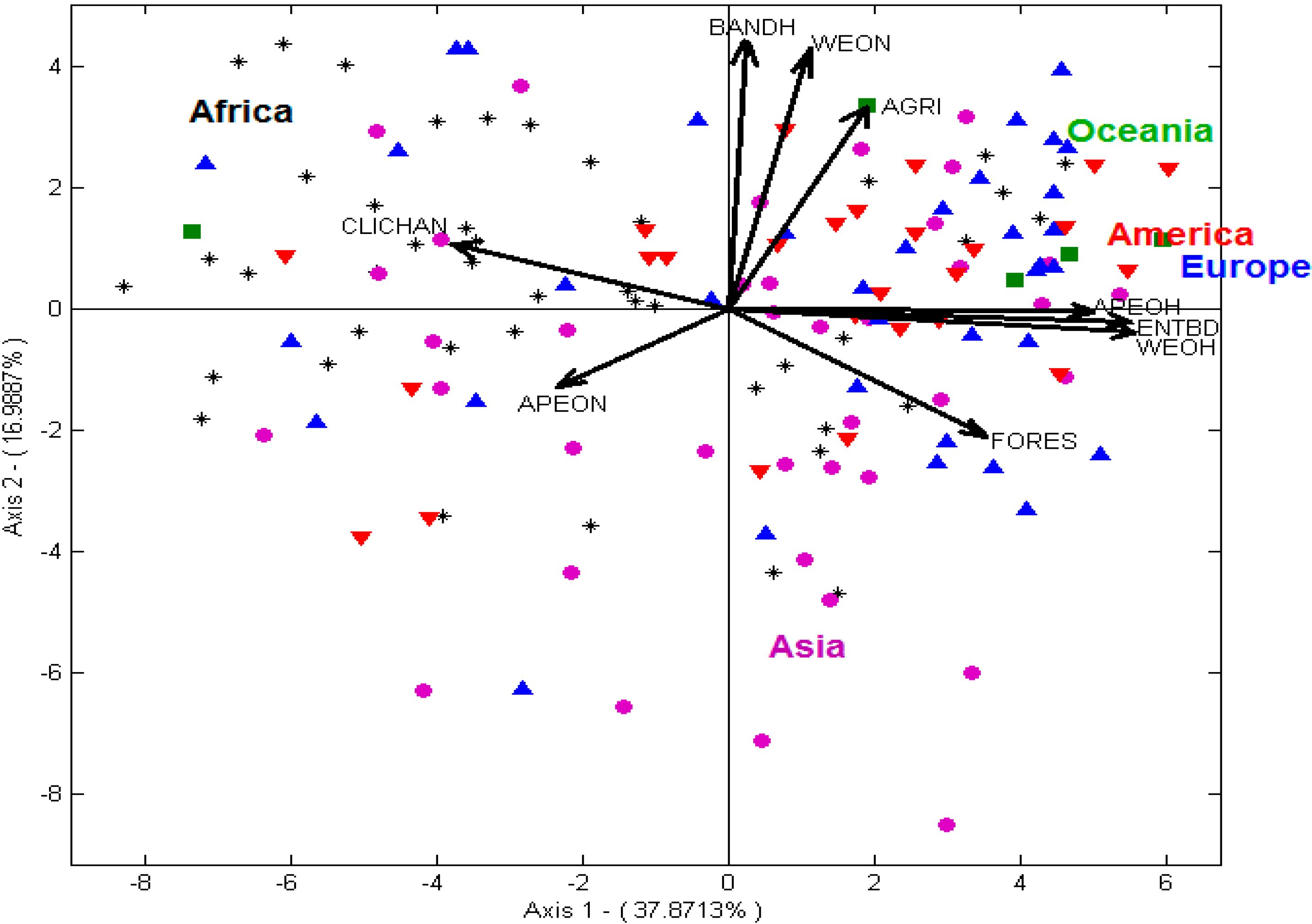
In addition to the initial model, the findings obtained by applying the biplot methodology add more detail, as two easily identifiable slopes were obtained: the variables close to Axis 1 or the horizontal axis (representing environmental health) and the variables close to Axis 2 or the vertical axis (representing ecosystem vitality). Given that the Environmental Performance Index (EPI) is also divided into two dimensions that coincide exactly with these slopes, we broke down the initial regression model into two models, one in which the dependent variable is environmental health and the other in which the dependent variable is ecosystem vitality. Thus, a better understanding is achieved of how the different explanatory variables affect the two large components of the environmental performance index.

It was observed that when the dependent variable is environmental health (see Table 6), it makes for a better model and confirms our initially posited H1 and H2 (economic wealth and education are the variables that most affect the environmental health of countries). In this sense, rich and developed countries are more likely to have access to the public funds needed to carry out environmental policies. This may be because their citizens demand higher environmental quality when it affects them directly, especially as concerns health-related pollutants; however, when the environmental aspect refers more to ecological or natural resources and factors, such as climate change, biodiversity, and so on, economic wealth as represented by the variable GDP per capita does not behave statistically in the same way, as it is negatively related to ecosystem vitality. That is, when economic wealth increases, ECOSVITALITY decreases, so it could be argued that many wealthy countries do not perform especially well on energy, climate, water stress, biodiversity, etc. The result we obtain when environmental performance is separated into its two components, environmental health and ecosystem vitality, are consistent with the findings by Jahn [23], who considers that although wealthy countries may be able to invest money in order to improve their environment in contrast to poorer countries, they also tend to create environmental problems owing to the their high level of consumption, which can lead to an increase in their pollution levels, thereby also generating more waste and using up more natural resources. Thus, Jahn [23] found that in rich countries, such as Germany, Japan, Canada, the United States and Switzerland, there was no relation between a country being wealthier and environmental performance.

With respect to the model used to predict EKC theory, according to Fiorino [28], the research studies derived from EKC recognize the critical role of political and governance factors in explaining environmental performance. This same author postulates that the results of EKC studies should be interpreted with caution, since the dependent variable can consider different indicators; it likewise depends on the type of country, since a developing country need not behave in the same way as other countries, and the economy-environment relationship is not predetermined.

7. Conclusions

The aim of this study was to analyze the following aspects. In the first place, we use economic and institutional variables jointly, in contrast to previous works that only use one type of variable, either economic or institutional, or present only a theoretical perspective. Secondly, we have contextualized the countries and variables (environmental indicators) using the biplot methodology, which provided a graphic representation that differentiates between countries’ environmental performance in relation to environmental health, on the one hand, and to ecosystem vitality, on the other. This classification happens to coincide with the division of dimensions in the environmental performance index (EPI). Thirdly, we ran different dependence models to verify which economic and institutional variables have the most impact on environmental performance according to the EPI, finding that economic variables, such as GDP and educational level, play a fundamental role in environmental performance and its components, especially in environmental health. Finally, we tested a model in which one of the variables is used in its quadratic form, specifically GDP (GDP²), and the results allow us to confirm EKC theory, which means that in the early stages of economic development, environmental performance increases along with income level, but then decreases in relation to growth in GDP at higher income levels.

In regard to the theories discussed—economic theory, ecological Kuznets curve theory and ecological modernization theory—as we have just seen, EKC is confirmed with the data used; economic theory is also confirmed, since as Jahn [23] points out, countries with greater economic growth are better able to handle environmental problems, because they have the financial resources to do so, and in our study, the GDP variable, which represents a country’s level of income, is statistically significant. However, we found no statistically significant evidence for the ecological modernization theory, which incorporates in addition to economic growth other variables, such as the role of science and technology, the importance of market dynamics, the role of economic agents and the ideology of social movements. These additional variables were either not used in our study or turned out not to be statistically significant, as in the case of political ideology.

In light of this latter finding, a possible future line of research would be to add these variables to the model. One could also broaden the sample to include more years for a longitudinal study and, in short continue a line of research on this topic in an attempt to ensure environmental sustainability, one of the priorities of environmental authorities around the world.

The results obtained have real-world applications and can be useful for policy makers. Hence, governments in different countries should make a greater effort to control corruption, since it reduces a country’s income, and low income levels can lead to higher levels of pollution, with the consequent decrease in environmental performance. Governments should also address educational concerns, because if a country’s income is not high enough for good sustainability, then good education may be the next best thing. Population density is also an important factor to consider in attaining good environmental performance, as we can deduce from our research: since there are many different countries, the population density is very high and heterogeneous in comparison to other research studies using fewer countries and in which population density has a positive effect on environmental performance. It can therefore be said that improvements in environmental performance may be best achieved by limiting future increases in population density. Another aspect to consider is that income is not the only explanatory variable for understanding environmental orientation and sustainability across countries; institutional factors must also be taken into account, since they can affect environmental performance indicators. Another important aspect is regime type: democratic regimes show higher levels of environmental performance than authoritarian regimes. These results can be attributed to the availability of information, opportunities to demonstrate and the independence of scientific researchers. High levels of democracy are also associated with growth in per capita income. However, governments should also take into account that being a wealthy country does not always lead to better environmental performance, especially when the environmental health aspect is considered apart from natural or ecological resources. Where the former is concerned, it can be affirmed that there is a positive and significant relation between wealth and environmental performance, but in the latter case, there is either no relation or else it is negative. The reason for this may be that although wealthy countries may be able to invest money in order to improve their environment in contrast to poorer countries, they also tend to create environmental problems owing to their high level of consumption. They have higher pollution levels, thereby also generating more waste and using more natural resources. What is certain is that effective governance leads to better environmental performance; according to Fiorino [28], effective, innovative and adaptable governance is a necessary condition for countries seeking a transition to sustainability. Among these aspects of governance to be considered are integrating policies, enhancing social capital, improving participation and making and implementing choices more adaptively.