1. Introduction
Public transit is considered to be one of the most important strategies of urban development in China because of its high capacity, low resource consumption, and environmental friendliness. Since 1985, the Chinese State Council has emphasized the necessity and importance of vigorous transit development [
1]. The primary reason for the poor quality of bus service in 1985 was the lack of buses. There were only 43,000 buses [
2] in the country, which was 1/11 of the buses in 2013. In 2004 [
3] and 2005 [
4], the Chinese Ministry of Construction and State Council required local governments to execute public transport priority strategy in succession. In 2006 [
5], the National Development and Reform Commission published the economic safeguard policy to stimulate public transport development. It required that local governments establish the preferential investment policy and fiscal subsidy mechanism for public transit.
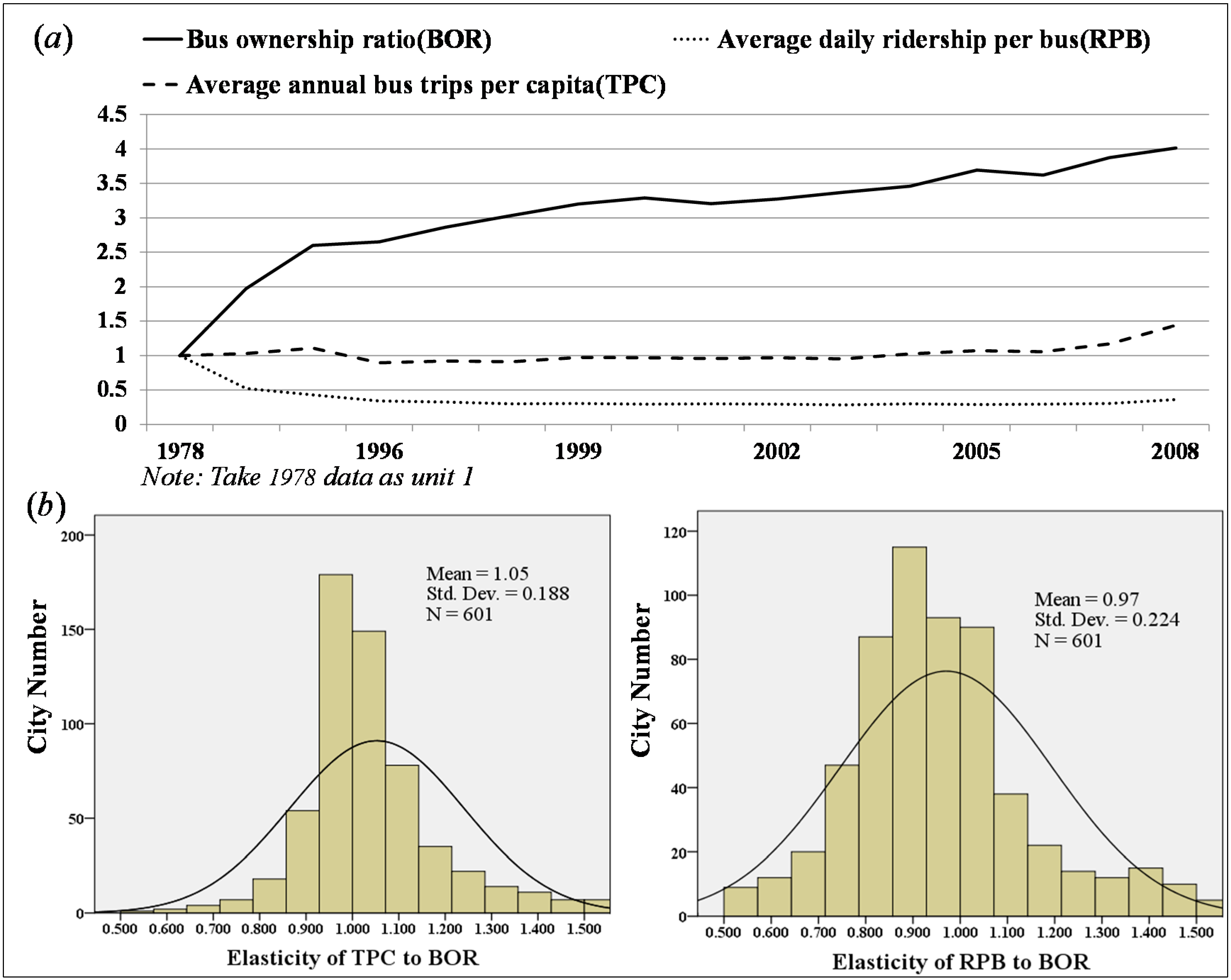
Due to the priority policy, the scale of the bus system in Chinese cities increased rapidly. The amount of buses increased by 13 times during 1978–2008,
i.e., 9.2% per year. Bus ridership was 6.7 billion in 2008, which is five times the rate in 1978, at 5.6% per year [
3]. However, growth of facility and ridership did not occur at the same pace. Several problems that deserve further attention appeared: (1) the residents’ willingness to travel by bus was not consistent with the increase of bus system capacity; (2) the bus system suffered from low operational efficiency due to an excess of buses; (3) the increase of bus fleet size meant varying performances in different cities.
It can therefore be surmised that governmental investment does not improve willingness to travel. Instead, the operational efficiency of a bus system decreases due to the excessive investment in the size of bus fleet. At present, some bus systems perform well both in willingness to travel and operational efficiency, while other cities only perform well in one aspect or in neither aspect. An invariable strategy for all the cities in China will lead to an output–input ratio. In order to improve the investment efficiency, a differentiated strategy based on actual bus system performance is necessary, and it will contribute to the development of policies of bus systems specific to different city types.
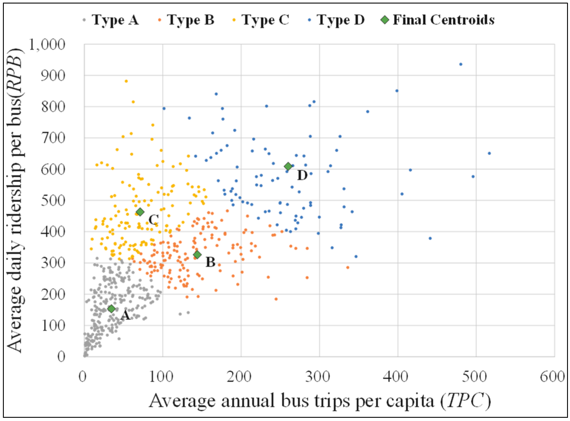
In this paper, two indicators—the annual average bus trips per capita (TPC) and average daily ridership per bus (RPB)—are used to describe the willingness to travel by bus and the operational efficiency of the bus system. All the cities in China are classified into four types by these two indicators, based on the K-Means Clustering method. Variable coefficient models are established to analyze the different impacts of urban geography, urban economy and bus system facility on these two indicators by using the statistical data from 645 Chinese cities during 2002–2008. Finally, the effective development strategies for different city types are proposed.
2. Literature Review
In recent years, many studies have analyzed the impacts of bus ridership with a number of variables such as transit fare, bus network structure, bus ownership, gasoline price, population, income,
etc. [
6,
7]. Taylor
et al. categorized variables into two types: external and internal variables [
8]. External variables are largely exogenous to the bus system, including geography, population, economy, transportation,
etc. Internal variables are under the control of bus operators, involving fares, bus network structure, bus ownership,
etc. Some studies have agreed on the positive or negative effects on bus ridership. For instance, bus facility scale and population density both have positive effects [
9,
10], whereas fare has negative effects [
11,
12].
However, there are discrepant opinions about the extent of the influence. For example, Nuworsoo [
13] and Bureau [
14] believe the internal variables such as fares and travel speed play a more crucial role; Holmgren [
15] and Frondel [
16], on the other hand, argue that external variables including income, population density and fuel prices have an even greater effect. Some studies have shown that the same variable has different results in different cities. Lago
et al. [
17] indicate that small-city bus ridership is more sensitive to fare than metropolitan. Bresson
et al. [
18] find that income has a stronger negative impact on bus ridership in England than in France due to the different demographic characteristics. Conversely, Sun and Zhou [
19] suggest that income growth has positive effects on bus ridership in China.
The different results can be summarized in three aspects: (1) different cities face different bus system development problems so the main variables diverge. Some cities suffer from the lack of bus facilities, whereas the main problem for some others comes from external variables such as low population; (2) some studies used a small sample, meaning that the results are not universal and only valid in the sample city [
20]; and (3) the multicollinearity of variables would also lead to contradictory conclusions.
Panel data is a combination of time series and cross-sectional data, and possesses the ability to deal with multicollinearity [
21]. As compared with time series data, panel data with a large cross-section size can reduce the effect of false regression that leads to unstable sample data [
22]. Moreover, panel data is able to describe changes over time, whereas cross-sectional data cannot. Panel data has been widely used in public transit research including fare structure [
23], subsidies [
24], ridership [
25],
etc.Ridership is an important index to reflect bus system performance, but the increase of ridership may be caused by t external variables, such as urban population growth rather than the improvement of public transit system; bus ridership can therefore not be used alone to portray the problems of a given bus system. A well-performed bus system should appeal to the citizens, thus the willingness to travel by bus provides a more suitable variable representing the improvement of a bus system [
26]. In addition, operational efficiency has to be considered because an oversized bus scale would cause large operational costs [
27,
28], thereby obstructing its further development.
In summation, although various internal and external variables in the literature have been analyzed for their impacts on bus ridership, different conclusions have been made due to different bus system development problems, small sample sizes, and unsuitable statistical methods. Although ridership is an important index of bus system performance, it cannot accurately reflect the deficiency of an existing system. Willingness to travel by bus and the operational efficiency of a bus system should therefore be taken into consideration when analyzing bus system performance.
3. Data and Method
3.1. Data Source
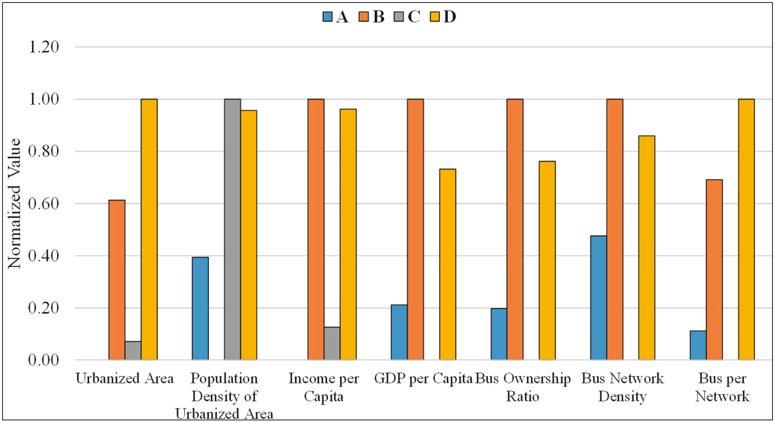
The first part of the analysis is to determine which variables have significant effects on Chinese bus system performances. According to previous research, seven variables have been selected and placed under three rubrics. The external variables include: (1) urban geography: urbanized area, population density of urbanized area; (2) urban economy: income per capita, GDP per capita; and, for the internal variables, (3) bus system facility, including: bus ownership ratio, bus network density, and bus per network.
The data for the paper is assembled from several sources. The primary bus system-related data comes from The China Urban Construction Statistical Yearbook, which is compiled annually by the Department of Integrated Finance, Ministry of Construction. This yearbook is based on statistical data of urban construction each year that is reported by construction authorities at the local levels of province, autonomous regions and municipalities directly under the central government. Urban economic data has been selected from The China City Statistical Yearbook, which is compiled annually by the Department of Urban Social and Economic Survey, National Bureau of Statistics. These two yearbooks contain almost all cities in China.
All relevant variables for 600 cities are collected from these two yearbooks (as seen in
Table 1). In 2008, the authority of urban bus systems transferred from the Ministry of Construction to the Ministry of Communications and the data referencing changed in 2009. For the purpose of keeping data consistent, this paper’s study period is thus from 2002 to 2008.
In order to complement some missing data, several provincial statistical yearbooks have been used, such as The Jiangsu Statistical Yearbook, The Guangdong Statistical Yearbook, etc. For the comparisons in this paper, income and GDP variables are converted into US dollars, on the basis of the 2008 exchange ratio: 6.94 Yuan per US dollar.
Table 1.
Relevant variables description.
Table 1.
Relevant variables description.
| Category Variable | Abbreviation | Variable Source/Construction | Unit |
|---|
| Urban population | | China Urban Construction Statistical Yearbook | 104 people |
| Urbanized area * | UA | China Urban Construction Statistical Yearbook | km2 |
| Total bus ridership | | China Urban Construction Statistical Yearbook | 104 passengers |
| Standard bus number | | China Urban Construction Statistical Yearbook | vehicle |
| Length of bus network | | China Urban Construction Statistical Yearbook | km |
| GDP per capita * | GDPPC | China City Statistical Yearbook | US dollar |
| Income per capita * | IPC | China City Statistical Yearbook | US dollar |
| Population density of urbanized area * | PUA | Urban population/Size of urbanized area | people/km2 |
| Bus ownership ratio * | BOR | Standard bus number/10,000 Urban population | vehicle/104 people |
| Bus network density * | BND | Length of bus network/Size of urbanized area | km/km2 |
| Bus per network * | BPN | Standard bus number/Length of bus network | bus/km |
3.3. Method
3.3.1. Analytical Framework
Bus system performances vary among different cities, so the development strategy should depend on the specific problems the cities are facing.
For analyzing characteristics of the cities with diverse bus system performances, 645 cities have been divided into four types according to the national average value of TPC and RPB in 2008. Furthermore, the various characteristics have been discussed on urban geography, economy, road infrastructure and bus system facility.
Subsequently, panel data from the period of 2002–2008 is used for analyzing the major influential variables on bus system performance and the extent of the same variables’ different impacts on different city types. Finally, different bus system development situations are discussed for the sake of matching development strategies.
3.3.2. Panel Data Model
Panel data is a combination of time series and cross-sectional data. Compared with time series and cross-sectional models, the panel data model has several advantages: it can increase the sample accuracy of estimators because of large amounts of observations, whereas the panel data model can get more dynamic information than the cross-sectional model [
29,
30].
In order to analyze the different impacts of variables varying from city to city, a variable coefficient model is established for each of the variables. In each model, only one variable is considered because of the “wide and short” panel data type (the cross-section is large, i.e., 645 cities, while the time period is short, i.e., only seven periods). The coefficient of one variable changes through the cities. Thus, the different effects of the variable among different cities can be analyzed.
The general formulation of the model is as follows:
where
k means the number of the effective variables (
i.e.,
UA,
PUA,
et al.);
i means the number of cities;
y means
TPC or
RPB;
x means the effective variable; α means the variable coefficient;
c means the intercept; and
u means the disturbing item.
5. Diversity of Bus System Development
5.1. Determinants of Bus System Development
5.1.1. Variable Preparation
Panel data from 2002 to 2008 are used to analyze the evolution of bus systems. The abbreviation of each variable is as follows: urbanized area (UA), population density of urbanized area (PUA), income per capita (IPC), GDP per capita (GDPPC), bus ownership ratio (BOR), bus per network (BPN), and bus network density (BND). All the variables undergo natural logarithmic transformation and then the coefficients turn to elasticity of the corresponding variables.
If data from a specific year is missing, the average values from the prior and following years are used as substitution. If the data from a particular city is missing for two consecutive years, for sake of accuracy none of that city’s data will be used. In the end, 264 cities’ data was available.
The cities in 2002 are classified according to the four final centroids from 2008. The nearest centroid based on Euclidean distance determines the city type. For example, if the Euclidean distances of city i, which considers TPC and RPB, from the A, B, C, D final centroids are 66, 79, 55, 103, respectively, then city i can be classified into type C due to the shortest Euclidean distance.
5.1.2. Choice of Model Type
The model type of the panel data needs to be decided before model-establishing. The model type includes variable intercept model, variable coefficient model and pooled regression model. The analyzing method is based on F-statistic test.
First, there are two assumptions.
If H1 is accepted, the model type will be the pooled regression model. If H1 is rejected, H2 needs to be tested. If H2 is accepted, the model type is the variable intercept model; otherwise the model type is the variable coefficient model.
The F-statistic value of H1 and H2 can be calculated like below:
where
S1,
S2 and
S3 means sum squared residual error of variable intercept model, variable coefficient model and pooled regression model, respectively;
N means the size of the cross-section;
T means the length of the time series; and
k means the number of independent variables. In this study, the model is established for each variable separately, therefore
k = 1. The time period is from 2002 to 2008, thus
T = 7. The available sample size is 264, hence
N = 264. The confidence level has been set as 95% and the critical values of F-statistic for
F1 and
F2 are 1.13 and 1.16, respectively.
The squared residual error and F-statistic values for different
TPC models are shown in
Table 4:
Table 4.
F-Statistic value of the TPC model.
Table 4.
F-Statistic value of the TPC model.
| Items | UA | PUA | IPC | GDPPC | BOR | BND | BPN |
|---|
| S1 | 1530.18 | 1309.90 | 1314.59 | 1306.25 | 1140.19 | 2260.18 | 2232.23 |
| S2 | 1910.44 | 1712.34 | 1688.32 | 1690.00 | 1499.89 | 2937.75 | 3022.78 |
| S3 | 5256.73 | 6365.58 | 5313.70 | 5371.86 | 3245.33 | 5528.97 | 4598.13 |
| F1 | 6.11 | 9.69 | 7.63 | 7.81 | 4.63 | 3.63 | 2.66 |
| F2 | 1.25 | 1.54 | 1.43 | 1.47 | 1.58 | 1.50 | 1.78 |
The squared residual error and F-statistic values for different
RPB models are shown in
Table 5:
Table 5.
F-statistic value of RPB.
Table 5.
F-statistic value of RPB.
| Items | UA | PUA | IPC | GDPPC | BOR | BND | BPN |
|---|
| S1 | 918.98 | 895.64 | 886.49 | 883.07 | 1140.19 | 1252.05 | 1397.87 |
| S2 | 1302.13 | 1301.53 | 1266.23 | 1268.41 | 1699.89 | 1623.10 | 1778.15 |
| S3 | 2990.025 | 3254.284 | 3014.343 | 3130.449 | 3245.331 | 3061.027 | 2972.747 |
| F1 | 5.66 | 6.61 | 6.02 | 6.39 | 4.63 | 3.63 | 2.83 |
| F2 | 2.09 | 2.27 | 2.15 | 2.19 | 2.46 | 1.49 | 1.37 |
In each model, F1 and F2 are larger than the critical values of F-statistic; both assumptions, H1 and H2, are therefore rejected. The variable coefficient model is selected.
5.1.3. Results Analysis
The results of the variable coefficient model are shown below:
- ●
TPC
Table 6.
Statistic results of TPC variable coefficient model.
Table 6.
Statistic results of TPC variable coefficient model.
| Item | UA | PUA | IPC | GDPPC | BOR | BND | BPN |
|---|
| R-squared | 0.76 | 0.80 | 0.79 | 0.79 | 0.82 | 0.61 | 0.61 |
| Adjusted R-squared | 0.71 | 0.75 | 0.75 | 0.75 | 0.78 | 0.53 | 0.52 |
| S.E. of regression | 0.71 | 0.65 | 0.66 | 0.66 | 0.61 | 0.88 | 0.89 |
| Sum squared resid | 1530.18 | 1309.90 | 1314.59 | 1306.25 | 1140.19 | 2260.18 | 2232.23 |
| Log likelihood | −3623.77 | −3335.05 | −3329.24 | −3311.89 | −3073.68 | −4248.27 | −4150.62 |
| F-statistic | 15.10 | 18.44 | 18.10 | 18.04 | 21.63 | 7.23 | 6.70 |
| Prob(F-statistic) | 0.00 | 0.00 | 0.00 | 0.00 | 0.00 | 0.00 | 0.00 |
As shown in
Table 6, the seven variables in each model are significant. The coefficients reflect their different impacts in different cities. In order to analyze the different impacts on
TPC among city types, the average coefficient is shown in
Table 7:
Table 7.
Average coefficients of TPC variable coefficient models.
Table 7.
Average coefficients of TPC variable coefficient models.
| City Type | Average Coefficient |
|---|
| UA | PUA | IPC | GDPPC | BOR | BND | BPN |
|---|
| A | 0.75 | 1.03 | 0.91 | 0.78 | 1.37 | 0.84 | 1.18 |
| B | 0.65 | 1.05 | 0.76 | 0.66 | 0.42 | 0.82 | 0.60 |
| C | 0.70 | 1.04 | 0.93 | 0.81 | 1.39 | 1.37 | 1.32 |
| D | 0.69 | 1.06 | 0.85 | 0.76 | 1.10 | 0.90 | 0.84 |
5.1.3.1. Urban Geography
UA and PUA both have positive impacts on willingness to travel by bus. It indicates that during the expansion of urbanized areas and the increase of population density, there will be more people that prefer to travel by bus. Types A and C have smaller urbanized areas than types B and D, thus more people in type A and C cities would choose the bus over non-motorized travel modes when trip distance increases; for this reason, the average coefficient of types A and C is a little larger than for types B and D. The population density of an urbanized area also has positive impacts on willingness to travel by bus because during the urbanization process, more people move from rural areas into urbanized ones, and this group of people prefers to travel by bus due to low income. According to the coefficient value, PUA almost has the same impacts on different city types.
5.1.3.2. Urban Economy
IPC and
GDPPC both have positive impacts on to travel by bus. The increase of
IPC means people can afford bus travel. The increase of
GPDPPC indicates that the local government can invest more into the bus system. Types A and C have relatively poorer economic conditions compared to types B and D (as seen in
Table 3), thus their improvements on
IPC and
GDPPC have a stronger impact on willingness to travel by bus than types B and D.
5.1.3.3. Bus System Facility
BOR,
BND and
BPN all have positive impacts on willingness to travel by bus. It is clear that the improvement of bus system facility promotes
TPC. However, it is worth mentioning that the impacts among city types vary. The increase of
BOR has the strongest effect on types A and C, which suffer from lack of bus vehicles (as seen in
Table 3 and
Figure 3). Although the increase of
BOR also has a positive impact on type B, the impact degree is narrower than the other three city types due to its oversized scale of buses (as seen in
Table 3 and
Figure 3). The largest coefficients of type C also indicate that type C would benefit the most from improvements in bus system facility.
Table 8.
Statistic results of RPB variable coefficient model.
Table 8.
Statistic results of RPB variable coefficient model.
| Items | UA | PUA | IPC | GDPPC | BOR | BND | BPN |
|---|
| Intercept | 4.69 | 6.45 | 2.84 | 3.29 | 5.36 | 5.17 | 5.43 |
| R-squared | 0.72 | 0.73 | 0.73 | 0.73 | 0.65 | 0.59 | 0.53 |
| Adjusted R-squared | 0.66 | 0.67 | 0.67 | 0.67 | 0.58 | 0.51 | 0.43 |
| S.E. of regression | 0.55 | 0.54 | 0.54 | 0.54 | 0.61 | 0.66 | 0.70 |
| Sum squared resid | 918.98 | 895.64 | 886.49 | 883.07 | 1140.19 | 1252.05 | 1397.87 |
| Log likelihood | −2674.24 | −2626.59 | −2601.18 | −2591.40 | −3073.68 | −3191.37 | −3341.13 |
| F-statistic | 12.26 | 12.70 | 12.58 | 12.53 | 8.96 | 6.64 | 4.99 |
| Prob(F-statistic) | 0.00 | 0.00 | 0.00 | 0.00 | 0.00 | 0.00 | 0.00 |
As seen in
Table 8, the seven variables are significant in each
RPB variable coefficient model, and the average coefficients are shown in
Table 9:
Table 9.
Average coefficients of RPB variable coefficient models.
Table 9.
Average coefficients of RPB variable coefficient models.
| City Type | Average Coefficient |
|---|
| UA | PUA | IPC | GDPPC | BOR | BND | BPN |
|---|
| A | 0.35 | 0.16 | 0.30 | 0.26 | 0.33 | 0.54 | 0.24 |
| B | 0.10 | 0.19 | 0.23 | 0.18 | −0.16 | 0.68 | 0.08 |
| C | 0.41 | 0.05 | 0.34 | 0.29 | 0.37 | 0.69 | 0.69 |
| D | 0.29 | 0.13 | 0.26 | 0.22 | 0.29 | 0.71 | 0.71 |
5.1.3.4. Urban Geography
UA and PUA have positive impacts on bus operational efficiency. Bus operational efficiency has a positive correlation with willingness to travel, thus when UA and PUA increase, bus operational efficiency likewise improves. Moreover, when PUA increases, there are more people in the urbanized area, thereby benefiting bus operational efficiency.
5.1.3.5. Urban Economy
IPC and GDPPC have positive impacts on bus operational efficiency. The impacts chiefly come from improvements in willingness to travel.
5.1.3.6. Bus System Facility
BND and
BPN have positive impacts on bus operational efficiency. The increase of bus system facility can improve the operational efficiency in most cities due to positive impacts on willingness to travel by bus. However, when the cities already have an excess of buses, the continuous increasing will reduce operational efficiency. As seen in
Table 9, a negative sign can be found in
BOR for type B. It indicates that the increase of
BOR will reduce the operational efficiency in type B cities.
The seven variables discussed previously have different impacts (positive and negative) and different impact degrees on willingness to travel by bus and operational efficiency. Effective development strategies for different city types therefore need to be found so that limited public resources can be effectively utilized.
5.2. Recommended Development Strategies for Different City Types
Considering both
TPC and
RPB, the development situations varied between 2002–2008. More than half the cities (52%) developed well enough that both
TPC and
RPB increased (T+R+). However, 13% of the cities performed worse (T−R−). Another 31% of cities succeeded in improving
TPC, although
RPB decreased (T+R−). Interestingly, there 4% of the cities failed in
TPC, but improved in
RPB (T−R+). The growth ratios of bus systems in T+R+ cities are extremely instructional by demonstrating the discrepancy between strongly performing cities. The annual growth ratios of these cities are shown in
Table 10.
Table 10.
Annual growth ratio of strongly performing cities.
Table 10.
Annual growth ratio of strongly performing cities.
| Variables | Annual Growth Ratio of T+R+ |
|---|
| A | B | C | D |
|---|
| BOR | 11.3% | 3.8% | 14.6% | 6.1% |
| BPN | 3.5% | 2.3% | 4.6% | 1.2% |
| BND | 5.8% | 4.9% | 6.4% | 6.5% |
The annual average growth ratios of BOR, BPN and BND in strongly performing type A cities are 11.3%, 3.5% and 5.8%, respectively. The development priority of type A is maintaining a high rate of development. The first step is to increase the size of the bus fleet and expand the bus service scope; the bus service frequency can subsequently be improved. The bus system of type A should develop appropriately in advance.
The annual average growth ratio of BOR in strongly performing type B cities is only 3.8%, which is the lowest of the four city types. Due to its large bus fleet, the development of the bus vehicle scale for type B requires maintaining the existing scale or slowing growth. The priority is to expand the bus service area (the growth ratio of BND is 4.9%), and improve the service quality.
Type C cities have the largest growth ratio of BOR, BND and BPN, 14.6%, 4.6% and 6.4%, respectively. This type of city requires immediate development. The development of bus system capacity lags far behind the development of the city, and the first strategy for type C would be to increase the number of buses and expand the bus service area. Once this has been achieved, bus service frequency needs to be improved.
Type D cities have a median growth ratio for BOR and BND of 6.1% and 6.5%, respectively. The bus systems of type D already have a strong performance. With the increase in urban population, however, a corresponding growth of bus fleet and service area is still necessary. In addition, high service quality, such as internal cleanliness or politeness and warmth from bus drivers and conductors, would have added benefits.
6. Conclusions
This study aims to describe the different levels of performance of bus systems in Chinese cities, proposing specific development strategies for different city types. The cities are classified into four types based on willingness to travel by bus and the operational efficiency of the bus system.
By using 645 cities’ data in 2008, the characteristics of different city types are analyzed. It is found that the cities with low willingness to travel and operational efficiency (i.e., type A) has a small urbanized area, low population density, poor economic conditions, and an insufficient bus system facility; the cities with high willingness to travel but low operational efficiency (i.e., type B) have low population density, the best economic conditions and too many buses (e.g., the average bus ownership ratio of type B is 15.3 bus/10 people); the cities with low willingness to travel but high operational efficiency (i.e., type C) are similar to type A in the scale of urbanized area and economic conditions, while type C cities have the highest population density of an urbanized area and the worst bus system facility of the four city types; the cities with both high willingness to travel and operational efficiency (i.e., type D) have the largest urbanized area, highest population density, strongest economic conditions and most suitable bus system facility.
Using panel data from 2002–2008, a variable coefficient model is established to compare the impacts of different variables on willingness to travel and operational efficiency in different city types. It is found that urbanized area, population density, economic condition and bus system facility have positive impacts on willingness to travel in all city types. The increases of bus ownership ratio, bus network density and bus per network have the most significant impacts on the willingness to travel of type C. Meanwhile, most of the above variables have positive impacts on operational efficiency in all city types, except the bus ownership ratio of type B. Because of the excess bus vehicle number of type B, the continuous increase of the bus fleet leads to lower operational efficiency. Finally, based on the annual growth ratio of the cities that are both improved in willingness to travel and operational efficiency, the recommended development strategies for different city types has been proposed.
However, bus system performance would not only be influenced by scale expansion, but also by the maintenance of existing systems, such as improving infrastructure maintenance, implementing an operation management model, encouraging appropriate subsidy, giving driving priority on the road to buses, etc. The paper has focused on city characteristics and bus system scale expansion. Further research should analyze the influences of existing systems’ maintenance on willingness to travel and operational efficiency. It must be pointed out that fare cost, travel time by bus and waiting time have not been taken into consideration because of the lack of available data. When this data becomes available for many cities in China, these variables can then be considered in a future study.

