Can China’s Industrial SO₂ Emissions Trading Pilot Scheme Reduce Pollution Abatement Costs?

Abstract

This paper evaluates the effects of China’s industrial SO₂ emissions trading pilot scheme (SETPS) on the pollution abatement costs (PAC) from the past and future perspective. We apply the kernel-based propensity score difference-in-difference method to examine the effects of SETPS on the average pollution abatement costs (APAC) and the marginal pollution abatement costs (MPAC) based on the environment data from the industrial sector of 29 provinces in China over the period of 1998 to 2011. Our findings are that SETPS failed to reduce PAC as a whole. During 2002 to 2011, SETPS increased APAC by 1310 RMB per ton on average and had an insignificant negative effect on MPAC. Nevertheless, the conclusions would be markedly different if we separately investigated the effects of SETPS each year of the pilot period. The positive effects of SETPS on PAC started to appear since 2009, and SETPS significantly reduced both APAC and MPAC, especially in 2009 and 2011.

1. Introduction

China’s economy has maintained a high-rate of growth since the reform and opening up in 1978. Meanwhile, the environment has been deteriorating. In order to restore the environment, Chinese governments have adopted both traditional administrative measures (e.g., command-and-control regulations) and market-oriented policy instruments (e.g., tradable permit scheme) to ease the environmental pollution. China used to solely rely on a charging scheme by imposing mandatory pollution taxes on business firms. However, the charging scheme failed to curb the environmental pollution. Chinese governments thus attempted to take some more market-oriented measures to reduce industrial emissions of SO₂ and other pollutants. As a result, the SO₂ emissions trading pilot scheme (SETPS) was initiated in 2002. Four provinces (i.e., Shandong, Shanxi, Jiangsu and Henan), three municipalities (i.e., Shanghai, Tianjin and Liuzhou) and one business entity (i.e., China Huaneng Group) were selected as the emissions trading scheme pilot regions or entity, which were known as the “4 + 3 + 1” project. These pilot regions and entity were responsible for 18.5% of SO₂ emissions in the acid rain and SO₂ control zones and included 131 cities and 727 firms, including Shanghai and Jiangsu, which were among the most developed areas of China, Shandong, which suffered the most serious SO₂ pollution, Henan, which was the biggest industrial province in central China and had the largest population in China, Shanxi, which was one of the heavy industry and energy bases of China, Tianjin, which was also a typical industrial city, Liuzhou, which was a typical acid district, and China Huaneng Group, which possessed one tenth of the thermal power generation capacity in China.

SETPS has been in effect in China for nearly twelve years since 2002. Can it really reduce the pollution abatement costs (PAC)? How does one measure the PAC? In this paper, we choose the average pollution abatement costs (APAC) and the marginal pollution abatement costs (MPAC) of SO₂ to evaluate the effects of SETPS on the economic growth and environment improvement in China. APAC, a historical cost concept in a static or past perspective, reflects the economic costs per unit of emissions reduction under the current environmental technical level. While MPAC, a future cost concept in a dynamic or future perspective, reflects the abandoned economic output per unit of additional emission abatement under the Pareto optimal level, which is gained through improving the environmental technical efficiency of each province. SETPS would be proven effective in the past if it could reduce APAC in a real sense. Furthermore, SETPS would be effective in the future if it could reduce MPAC, and thus, the environmental technology efficiency of each province could achieve the Pareto optimal level.

In order to examine whether SETPS is effective in China, we apply the kernel-based propensity score difference-in-difference method to analyze the effects of SETPS on APAC and MPAC. The empirical evidence indicates that SETPS had failed to reduce PAC if the pilot period as a whole sample were taken into account. SETPS increased APAC by 1,310 RMB per ton on average from 2002 to 2011 and reduced MPAC by 72,400 RMB per ton on average, which was not significant. Nevertheless, the conclusion would be soundly different if we separately investigated the effects of SETPS each year of the pilot period. SETPS began to show positive effects on PAC since 2009 and significantly reduced both APAC and MPAC, especially in 2009 and 2011. Therefore, the effects of SETPS on reducing PAC are expected to be stable if the emissions permits trading market could be improved reasonably in the future.

The paper is unfolded as follows: Section 2 provides a literature review; Section 3 develops several theoretical models to measure MPAC and to evaluate the effects of SETPS; Section 4 introduces how the data were used in the research; Section 5 shows the empirical evidence; Section 6 serves as the conclusion of this research; the last section discusses the limitations of the paper and provides an outlook for further research on this subject.

2. Literature Review

Economists generally believe that the emissions permit trading scheme is a more effective measure than environmental taxes. Coase (1960) suggested that emission permits allocated through a market mechanism are the most efficient mechanism to solve pollution problems [1]. Crocker [2] (1966), Dales [3] (1968) and other researchers further pointed out that the emissions permit trading scheme is effective at dealing with external environmental resources. Montgomery [4] (1972) proved that market-oriented emissions trading schemes are superior to traditional environmental governance measures. Compared with traditional environmental governance measures, the emissions trading policy has an advantage in reducing PAC. Tietenberg [5] (1985) demonstrated it and argued that the emissions trading scheme reduces PAC by allowing these firms with high abatement costs to purchase emissions permits until the emissions trading market reaches equilibrium. This indicates that each firm’s marginal abatement costs are equal and that the social abatement costs will be reduced entirely through this process. Some scholars also found relevant evidence in empirical studies. Grubb [6] (2003) proposed that Annex I countries in the Kyoto Protocol can reduce emissions costs largely through the carbon emissions trading market. In addition, Rose et al. [7] (2006) examined the U.S. data and concluded that the more participants in the carbon emissions trading markets there are, the more cost-saving effects there will be.

China is a large country with huge emissions. Therefore, an increasing number of researchers have engaged themselves in studying the effects and rationality of China’s emissions trading. Among them are Li and Shen [8] (2008), Wang and Tu [9] (2009), He and Xiao [10] (2010), Zheng [11] (2010), Tan and Chen [12] (2012), Yan and Guo [13] (2012), etc. They demonstrated two unique opinions. One is An and Tang [14] (2012), who diverted the analysis on quota-based trading market in most literatures to the analysis on the project-based trading market [14]. The other one is Fan [15,16] (2012), who mainly focused on the consumption aspect of the emissions trading market, adhering to Ferng’s [17] (2003) idea that it is consumers, not producers, who should be blamed for driving up pollution in manufacturing sectors.

Cui et al. [18] (2013) proposed a provincial emissions trading model and concluded that in the effort to achieve the emission reduction targets of every province, a unified national carbon emissions trading market can save 23.44% in abatement costs, while a carbon emissions trading pilot market, which involves only six pilots, can save 4.42% when both are compared with the scenario of no carbon emissions trading. From a regional perspective, the cost-saving effects are much more significant in eastern and western China.

Nevertheless, the existing literature aiming at evaluating SETPS focuses primarily on the environmental impacts, such as emissions mitigation (e.g., total emissions reduction and/or emissions intensity mitigation), and rarely considers environmental and economic factors. Therefore, they are not in compliance with the core ideology of sustainable development. This paper argues that PAC is one of the best evaluation indexes when examining the effectiveness of emissions trading schemes. Cui et al. [18] (2013) applied this evaluation method. However, their research was based on simulation instead of the data from the emissions trading pilots in practice [18]. As a result, an evaluation approach with a “natural experiment” character was initiated in six pilot provinces in 2002, with Liuzhou and China Huaneng Group as an exception. This paper adopts thekernel-based propensity score difference-in-difference method to evaluate whether SETPS can reduce PAC or not. Differing from the other research up to now, this paper defines PAC in a much more comprehensive way by admitting that APAC reflects historical costs, while MPAC reflects future costs. In this case, we can evaluate the effects of SETPS on PAC in the past and future.

3. The Theoretical Underpinnings

3.1. How to Measure PAC

Following Li et al. [19] (2010), who divided the total environmental costs of industrial production into paid environmental costs and unpaid environmental costs [19], the paper divides SO₂ abatement costs into the following two categories. One is paid abatement costs, which refers to the abatement expenditure that industrial enterprises pay for desulfurization and other environmental treatments of SO₂ generated in the process of production. The other is unpaid abatement costs, which are the additional abatement costs or opportunity costs generated by reducing SO₂ emissions to the required levels by current environmental regulations. Therefore, this paper defines unpaid abatement costs to a small extent. This is slightly different from Li et al. [19] (2010), who define unpaid abatement costs as whole governance expenses needed under the current governance and technology level. These abatement costs are determined by the desulfurization rate and technology. Because the desulfurization rate is determined by the intensity of environmental regulations, the implementation of an environmental policy will indirectly affect PAC by changing the desulfurization rate. However, the economic development level and the size of the population are different across provinces in China. A difference within a certain spectrum in SO₂ emissions across provinces is considered reasonable. Therefore, it is reasonable to use unit or marginal costs rather than total costs when making a comparative analysis across provinces or cities in cross-sectional dimensions. Based on the above economic logic, this paper extends two categories of SO₂ abatement costs to average or marginal concepts, namely APAC and MPAC, in order to test the effectiveness of environmental policies. APAC is the paid abatement costs that take into account the investment in the treatment of industrial pollution in terms of per unit desulfurization. MPAC is the unpaid abatement costs, which are measured by network DEA in this paper. The following paragraph will focus on the measurement of MPAC.

Boyd et al. [20] (2002) and Chen [21] (2011) employed the directional distance function (DDF) to construct the formulas of MPAC by comparing command-and-control regulations with standard energy saving and emissions reduction regulations in terms of potential outputs and potential emissions However, according to Färe et al. [22] (2011) and Tu and Shen [23] (2013), this may cause a serious deviation, because the traditional measuring method of environmental technology efficiency underestimates environment governance efficiency. Therefore, there must be bias in the potential output and the potential emissions measured with the traditional method. In addition, an accurate MPAC could not be calculated. In accordance with the calculation methodology of Boyd et al. [20] (2002) and Chen [21] (2011), this paper builds a formula for MPAC by using the environmental directional distance function, which is based on network DEA proposed by Färe et al. [22] (2011) and Tu and Shen [23] (2013).

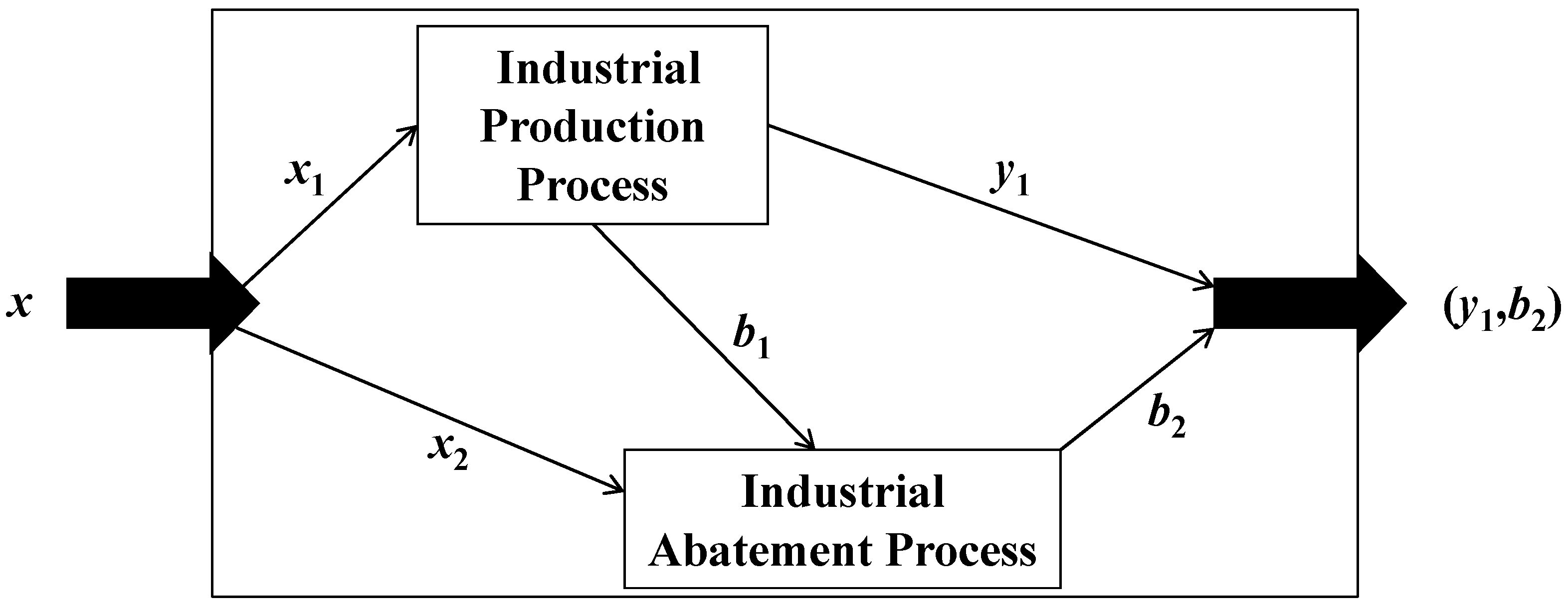
In accordance with the study of Färe et al. [22] (2011) and Tu and Shen [23] (2013), this paper divides the production process into two main phases: production and abatement, which are denoted as P₁ and P₂, respectively. When inserting input x₁ into the production process, we can get output y and pollution b₁. While, when inserting input x₂ into the abatement process, we can reduce pollution b₁ to pollution b₂. We illustrate this setup in Figure 1.

Figure 1. Industrial environmental technology based on network DEA.

Figure 1. Industrial environmental technology based on network DEA.

Define the environmental technology based on network DEA as:

$$P(x)=\{(y,b_2):(y,b_1)\in P_1(x_1),b_2\in P_2(x_2,b_1)\}$$

(1)

Thus, the directional environmental distance function based on network DEA can be expressed as:

$$\overrightarrow{N{D}_o^t}(y^t,x_1^t,x_2^t,b_2^t;g_y^t,-g_b^t)=\sup [\beta :(y^t+\beta g_y^t,b_2^t-\beta g_b^t)\in P^t(x^t)]$$

(2)

When implementing command-and-control regulations, we can choose directional vector $g^t=(y_1^t,0)$ , so that the directional environmental distance function based on network DEA can be calculated by solving the following mathematical programming if producer $k^{\prime }(y_{1,k^{\prime }}^t,x_{1,k^{\prime }}^t,x_{2,k^{\prime }}^t,b_{2,k^{\prime }}^t)$ takes reference technology P^t (x^t) into consideration:

$$\begin{array}{l}\overrightarrow{N{D}_o^t}(y_{1,k^{\prime }}^t,x_{1,k^{\prime }}^t,x_{2,k^{\prime }}^t,b_{2,k^{\prime }}^t;y_{1,k^{\prime }}^t,0)=\max {\beta }_c\begin{array}{ccc}& & \end{array}s.t.\\ \begin{array}{ccc}industrial& production& processs:\end{array}\\ \begin{array}{ccccccc}& & & & & & \end{array}{\displaystyle \sum _{k=1}^K{z}_{k_1}{y}_{1,k,m_1}^t\ge (1+{\beta }_c)y_{1,k^{\prime },m_1}^t},m_1=1,\cdots ,M_1,\\ \begin{array}{ccccccc}& & & & & & \end{array}{\displaystyle \sum _{k=1}^K{z}_{k_1}{b}_{1,k,j_1}^t=b_{1,k^{\prime },j_1}^t},j_1=1,\cdots ,J_1，\\ \begin{array}{ccccccc}& & & & & & \end{array}{\displaystyle \sum _{k=1}^K{z}_{k_1}{x}_{1,k,n_1}^t\le x_{1,k^{\prime },n_1}^t},n_1=1,\cdots ,N_1,\\ \begin{array}{ccccccc}& & & & & & \end{array}{z}_{k_1}\ge 0,k_1=1,\cdots K\\ \begin{array}{ccc}industrial& abatement& process:\end{array}\\ \begin{array}{ccccccc}& & & & & & \end{array}{\displaystyle \sum _{k=1}^K{z}_{k_2}{b}_{2,k,j_2}^t=b_{2,k^{\prime },j_2}^t},j_2=1,\cdots ,J_2,\\ \begin{array}{ccccccc}& & & & & & \end{array}{\displaystyle \sum _{k=1}^K{z}_{k_2}{b}_{1,k,j_1}^t\le b_{1,k^{\prime },j_1}^t},j_1=1,\cdots ,J_1\\ \begin{array}{ccccccc}& & & & & & \end{array}{\displaystyle \sum _{k=1}^K{z}_{k_2}{x}_{2,k,n_1}^t\le x_{2,k^{\prime },n_2}^t},n_2=1,\cdots ,N_2,\\ \begin{array}{ccccccc}& & & & & & \end{array}{z}_{k_2}\ge 0,k_2=1,\cdots K\end{array}$$

(3)

Now, we can get the potential output y_c:

$$y_c=(1+{\beta }_c)y$$

(4)

When enforcing standard energy saving and emissions reduction regulations, we can choose directional vector $g^t=(y_1^t,-b_2^t)$ , so that the directional environment distance function based on network DEA can be calculated by solving the following mathematical programming if producer $k^{\prime }(y_{1,k^{\prime }}^t,x_{1,k^{\prime }}^t,x_{2,k^{\prime }}^t,b_{2,k^{\prime }}^t)$ takes reference technology $P^t(x^t)$ into consideration:

$$\begin{array}{l}\overrightarrow{N{D}_o^t}(y_{1,k^{\prime }}^t,x_{1,k^{\prime }}^t,x_{2,k^{\prime }}^t,b_{2,k^{\prime }}^t;y_{1,k^{\prime }}^t,-b_{2,k^{\prime }}^t)=\max {\beta }_r\begin{array}{ccc}& & \end{array}s.t.\\ \begin{array}{ccc}industrial& production& processs:\end{array}\\ \begin{array}{ccccccc}& & & & & & \end{array}{\displaystyle \sum _{k=1}^K{z}_{k_1}{y}_{1,k,m_1}^t\ge (1+{\beta }_r)y_{1,k^{\prime },m_1}^t},m_1=1,\cdots ,M_1,\\ \begin{array}{ccccccc}& & & & & & \end{array}{\displaystyle \sum _{k=1}^K{z}_{k_1}{b}_{1,k,j_1}^t=b_{1,k^{\prime },j_1}^t},j_1=1,\cdots ,J_1，\\ \begin{array}{ccccccc}& & & & & & \end{array}{\displaystyle \sum _{k=1}^K{z}_{k_1}{x}_{1,k,n_1}^t\le x_{1,k^{\prime },n_1}^t},n_1=1,\cdots ,N_1,\\ \begin{array}{ccccccc}& & & & & & \end{array}{z}_{k_1}\ge 0,k_1=1,\cdots K\\ \begin{array}{ccc}industrial& abatement& process:\end{array}\\ \begin{array}{ccccccc}& & & & & & \end{array}{\displaystyle \sum _{k=1}^K{z}_{k_2}{b}_{2,k,j_2}^t=(1-{\beta }_r)b_{2,k^{\prime },j_2}^t},j_2=1,\cdots ,J_2,\\ \begin{array}{ccccccc}& & & & & & \end{array}{\displaystyle \sum _{k=1}^K{z}_{k_2}{b}_{1,k,j_1}^t\le b_{1,k^{\prime },j_1}^t},j_1=1,\cdots ,J_1\\ \begin{array}{ccccccc}& & & & & & \end{array}{\displaystyle \sum _{k=1}^K{z}_{k_2}{x}_{2,k,n_1}^t\le x_{2,k^{\prime },n_2}^t},n_2=1,\cdots ,N_2,\\ \begin{array}{ccccccc}& & & & & & \end{array}{z}_{k_2}\ge 0,k_2=1,\cdots K\end{array}$$

(5)

Now, we can get the potential output y_r and the potential pollution b_r:

$$y_r=(1+{\beta }_r)y$$

(6)

$$b_r=(1-{\beta }_r)b_2$$

(7)

The potential output and the potential pollution under different environmental policies are indicated in Figure 2. Point A represents the producer’s initial output and emissions. Producers can reach the frontier Point B by improving their technical efficiency under no environmental regulations. Producers can reach the frontier Point C by improving their technical efficiency and expanding production under command-and-control regulations with a given emissions level. Producers can reach the frontier Point D by improving their technical efficiency in the case of production expansion and emissions reduction under the standard energy saving and emissions reduction regulations in place. Comparing Point C with D, it is shown that producers may lose the potential output (y_c – y_r) for reducing the emissions (b – b_r) with standard energy saving and emissions reduction regulations rather than the command-and-control regulations in place. Therefore, in accordance with the methodology of Boyd et al. [20] (2002) and Chen [21] (2011), MPAC is calculated as follows:

$$M\text{P}AC=(y_c-y_r)/(b-b_r)=({\beta }_c-{\beta }_r)y/({\beta }_r{b}_2)$$

(8)

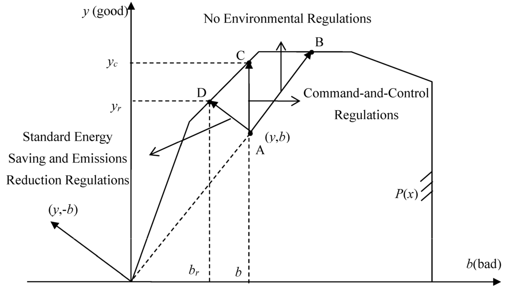
Figure 2. The potential output and potential emissions under different environmental schemes.

Figure 2. The potential output and potential emissions under different environmental schemes.

3.2. Kernel-Based Propensity Score Difference-in-Difference Method

In order to examine the effects of SETPS, we adopt the difference-in-difference method, which is normally used to assess the effectiveness of public policies. We regard SETPS as a policy experiment or natural experiment, the pilot provinces (i.e., Tianjin, Shanxi, Shanghai, Jiangsu, Shandong, Henan) as the treated group or experimental group, non-pilot provinces as the control group, the non-pilot period from 1998 to 2001 as the before treatment period and the pilot period from 2002 to 2011 as the after treatment period. As seen from the model, Y represents APAC and MPAC, and dummy variables period and treated denote period and province, respectively, whether SETPS is implemented or not. Therefore, we can formulate the regression model as follows:

$$Y_{it}={\beta }_0+{\beta }_{1}perio{d}_t+{\beta }_{2}treate{d}_i+{\beta }_{3}perio{d}_t\cdot treate{d}_i+{\mu }_{it}$$

(9)

In Model (9), β₃ examines the effects of SETPS on PAC (including APAC and MPAC) in the past and future. However, the pilot provinces are not randomly chosen, but determined by Chinese governments. It does not meet the requirements of random sampling of the treatment group (or experimental group) in the policy experiment (or natural experiment). Pilot provinces probably obtain this pilot opportunity because of some factors. Therefore, it is difficult to ensure that the PAC changes in both pilot provinces and non-pilot provinces from the non-pilot period to pilot period are due to the same reasons. On the contrary, it is possible that some specific factors cause different changes in PAC between the pilot provinces and non-pilot provinces. In this case, this will lead to a serious estimation bias if using the difference-in-difference method to directly estimate Model (9). The kernel-based propensity score difference-in-difference method is employed to solve this estimation problem in this paper. This estimation method consists of three steps. Firstly, the probit model (or logit model) is used to estimate the propensity score of the samples. Then, the principle of similar propensity score is obeyed to match one or more control groups with treatment groups (or experimental groups). Through this process, we can eliminate the self-selection problem of the treated group (or experimental group) to achieve random selection. Finally, with the matching results, the propensity score is used to formulate a weighting function based on the kernel density function. After that, we can calculate the effect of policy experiments (or natural experiments), namely β₃ estimated in Model (9).

The key issue to apply the kernel-based propensity score difference-in-difference method is to make a reasonable choice on the explanatory variables that determine the pilot provinces in SETPS. This paper considers the fact that Chinese governments may weigh over these six determinants (i.e., emissions intensity, energy intensity, GDP per capita, the proportion of industry sector in GDP, the proportion of urban population and the proportion of state-owned and state-holding industrial enterprises) to make the choice. These six determinants can be classified into three categories as follows:

• Environmental and energy factors: SO₂ emissions intensity (SI) and energy intensity (EIP). In general, the intensity of environmental regulations is determined by the basic conditions of the environment and energy of each province. Emission intensity refers to the SO₂ emissions per unit of energy consumption, which reflects the energy consumption structure. A low emission intensity indicates a large proportion of clean energy (e.g., hydropower, nuclear power and solar energy) or low-carbon energy in the total energy consumption. Energy intensity refers to the energy consumption per unit of the industrial gross output and reflects in the level of energy efficiency or energy-saving technology. A low energy intensity indicates a high energy efficiency or energy-saving technology.
• Macro-economic factors: GDP per capita (GDPP), the proportion of the industrial sector in GDP (industrialization) and the proportion of urban population (urbanization). These indicators reflect the economic development level, the industrialization level and the urbanization level, respectively. Generally speaking, the relatively developed regions are more inclined to implement SETPS.
• Micro-enterprise factor: the proportion of state-owned and state-holding industrial enterprises (state_rate). In terms of the cost-benefit function, the national protection level and the environmental constraints vary across state-owned enterprises and private enterprises (Yan and Guo, 2012) [13]; the efficacy of environmental policies will be significantly different across enterprises of different ownership. Meanwhile, a lower proportion of state-owned and state-holding industrial enterprises implies a higher degree of marketization and is also conducive to the implementation of market-oriented policies. Thus, the proportion of state-owned and state-holding industrial enterprises reflects the ownership structure, as well as the degree of marketization.

In summary, the probit model can be formulated as follows:

$$\begin{array}{l}P(treated=1|x)=\Phi ({\alpha }_{1}S{I}_i+{\alpha }_{2}EI{P}_i+{\alpha }_{3}GDP{P}_i+{\alpha }_{4}industrializatio{n}_i\\ \begin{array}{cc}& \end{array}+{\alpha }_{5}urbanizatio{n}_i+{\alpha }_{6}state\_rat{e}_i+{\nu }_i)\end{array}$$

(10)

4. Data

This study employs balanced panel data covering 29 provinces in China over the period from 1998 to 2011. The industrial enterprises of above designated size are examined as representative of China’s industrial sector in the empirical analysis. The Industrial enterprises of the above designated size are all state-owned enterprises and non-state owned enterprises with annual revenue from principal business over 5 million RMB from 1998 to 2006, and they are industrial enterprises with annual revenue from principal business over 5 million RMB from 2007 to 2010 and are industrial enterprises with annual revenue from principal business over 20 million RMB after 2011. Considering that Qinghai’s volume of SO₂ removed in the period of 2001–2006 was very small (close to 0 if we use units of tons) and that Tibet had lots of missing data, which would affect the relevant calculations in this paper, these two provinces are therefore excluded here. All kinds of data in this paper are obtained mainly from “China Statistical Yearbook from 1999 to 2012” [24], “China Energy Statistical Yearbook from 1997 to 2012 [25]”, “China Compendium of Statistics from 1949 to 2008” [26], “China Statistical Yearbook on Environment 2012” [27] and “China Industry Economy Statistical Yearbook from 2001 to 2012” [28].

The variables in this study are constructed in accordance with Tu and Shen [23] (2013). As for the industrial production process, we choose annual average of employees in the industrial sector (l), net value of the fixed assets in the industrial sector (k) and industrial end-use energy consumption (e) as input variables, while we use industrial gross output (y) as the output variable and the volume of SO₂ emissions by industrial production (s₁) as the emission variable. With regard to the industrial abatement process, we choose the volume of SO₂ emissions by industry production (s₁) and the number of facilities for the treatment of industrial waste gas (GMS) as input variables, while we use the volume of terminal SO₂ emissions by industry (s₂) as the output variable. Paid abatement costs are measured by the investment in the treatment of industrial pollution. Each province’s net value of the fixed assets in the industrial sector and investment in the treatment of industrial pollution are converted into the comparable value, with 1998 as the base year, by using the price index of investment in fixed assets. The industrial gross output and the output of state-owned and state-holding industrial enterprises of each province are also converted into the comparable value, with 1998 as the base year, by using the producer price index for industrial products. Four indicators of industrial enterprises of the above designated size, which are volume of terminal SO₂ emissions, volume of SO₂ removed, end-use energy consumption and number of facilities for treatment of wastes gas, have not been released. Considering that the industrial enterprises of the above designated size account for a large proportion of the industrial sector, we use industrial-level data instead.

The economic data in this study are collected mainly from “China Statistical Yearbook” [24] and partly from “China Compendium of Statistics from 1949 to 2008” [26] and “China Industry Economy Statistical Yearbook from 2001 to 2012” [28]. Meanwhile, missing data are filled by using the linear interpolation method. As for the specific process of industrial end-use energy consumption (please see Tu and Shen [29] (2013)), this paper uses the sum of 20 kinds of end-use energy consumption. In addition, the data on GDP per capita, the proportion of the industrial sector in GDP and the proportion of urban population are sourced from Tu and Shen [29] (2013).

Table 1 gives a brief statistical description of the final sample in terms of output, input and price variables.

Table 1. Statistical description of outputs, inputs and prices variables.

Variable	Observations	Mean	SD	Min	Max
Investment in the Treatment of Industrial Pollution (100 million RMB)	406	4.44	4.70	0.01	33.71
Industrial Gross Output (100 million RMB)	406	9644.52	14,826.62	183.20	93,960.53
Producer Price Indices for Industrial Products (1998 = 1)	406	1.11	0.25	0.85	2.56
Net Value of the Fixed Assets in Industrial Sector (100 million RMB)	406	3032.35	2833.34	181.37	16,896.21
Price Indices for Investment in Fixed Assets (1998 = 1)	406	1.15	0.15	0.96	1.56
Annual Average of Employees in Industrial Sector (10,000 persons)	406	244.20	255.58	11.60	1,568.00
Industrial End-use Energy Consumption (10,000 tons of standard coal equivalent (SCE)	406	3335.09	2773.92	67.46	16,285.17
Number of Facilities for Treatment of Industrial Wastes Gas (set)	406	5348.20	3449.14	292.00	21,702.00
Volume of SO2 Emissions by Industry Production (10,000 tons)	406	115.12	84.93	2.11	592.88
Volume of Terminal SO2 Emissions by Industry (10,000 tons)	406	62.54	38.72	1.93	176.01
Emissions Intensity (ton/ton of SCE)	406	0.02	0.01	0.00	0.08
Energy Intensity (ton of SCE/10,000 RMB)	406	0.76	0.68	0.06	8.47
GDP per Capita (10,000 RMB/person)	406	1.43	1.07	0.22	6.13
The Proportion of Industry Sector (%)	406	42.75	9.34	12.68	63.29
The Proportion of Urban Population (%)	406	45.02	16.21	19.93	89.30
The Proportion of State-owned and State-holding Industrial Enterprises (%)	406	50.16	20.70	10.73	89.88

Table 1. Statistical description of outputs, inputs and prices variables.

Variable	Observations	Mean	SD	Min	Max
Investment in the Treatment of Industrial Pollution (100 million RMB)	406	4.44	4.70	0.01	33.71
Industrial Gross Output (100 million RMB)	406	9644.52	14,826.62	183.20	93,960.53
Producer Price Indices for Industrial Products (1998 = 1)	406	1.11	0.25	0.85	2.56
Net Value of the Fixed Assets in Industrial Sector (100 million RMB)	406	3032.35	2833.34	181.37	16,896.21
Price Indices for Investment in Fixed Assets (1998 = 1)	406	1.15	0.15	0.96	1.56
Annual Average of Employees in Industrial Sector (10,000 persons)	406	244.20	255.58	11.60	1,568.00
Industrial End-use Energy Consumption (10,000 tons of standard coal equivalent (SCE)	406	3335.09	2773.92	67.46	16,285.17
Number of Facilities for Treatment of Industrial Wastes Gas (set)	406	5348.20	3449.14	292.00	21,702.00
Volume of SO2 Emissions by Industry Production (10,000 tons)	406	115.12	84.93	2.11	592.88
Volume of Terminal SO2 Emissions by Industry (10,000 tons)	406	62.54	38.72	1.93	176.01
Emissions Intensity (ton/ton of SCE)	406	0.02	0.01	0.00	0.08
Energy Intensity (ton of SCE/10,000 RMB)	406	0.76	0.68	0.06	8.47
GDP per Capita (10,000 RMB/person)	406	1.43	1.07	0.22	6.13
The Proportion of Industry Sector (%)	406	42.75	9.34	12.68	63.29
The Proportion of Urban Population (%)	406	45.02	16.21	19.93	89.30
The Proportion of State-owned and State-holding Industrial Enterprises (%)	406	50.16	20.70	10.73	89.88

5. Main Empirical Results

5.1. APAC and MPAC

Since the paid abatement costs are measured in terms of the investment in the treatment of industrial pollution, APAC is calculated in terms of the paid abatement costs per unit of desulfurization. Based on the network DEA to measure the MPAC proposed above, we make an estimation on the MPAC for each province in China from 1998 to 2011. By contrast, we also use the traditional method, namely DDF, to measure MAC, and we find that there is a significant difference between the two results. Please see the Appendix,

Table A1. Comparison of MPAC estimated by network DEA and the directional distance function (DDF) (units: 10,000 RMB/ton).

Province/City	MPAC	1998	1999	2000	2001	2002	2003	2004	2005	2006	2007	2008	2009	2010	2011	Mean
Beijing	1	0.00	0.00	0.00	0.00	0.00	0.00	0.00	0.00	0.00	0.00	0.00	0.00	0.00	0.00	0.00
	2	−12.66	108.37	2.39	253.40	0.00	363.96	0.00	0.00	0.00	0.00	0.00	0.00	0.00	0.00	51.10
Tianjin	1	0.00	0.00	0.00	0.00	0.00	0.00	0.00	0.00	0.00	0.00	0.00	0.00	0.00	0.00	0.00
	2	−9.45	122.60	−29.60	39.60	49.67	−20.13	−20.68	0.00	0.00	0.00	0.00	0.00	0.00	0.00	9.43
Hebei	1	0.00	0.00	0.00	0.00	0.00	0.00	0.00	0.00	0.00	0.00	0.00	0.00	0.00	0.00	0.00
	2	−6.31	−11.51	−14.25	−13.72	−15.49	−10.57	−20.68	−30.14	−28.43	−36.99	−58.05	−62.37	−86.03	−75.20	−33.55
Shanxi	1	0.94	1.46	2.74	3.92	6.21	6.68	8.84	13.53	27.19	24.61	37.70	43.06	16.84	23.82	15.54
	2	1.06	3.09	2.47	2.21	7.26	10.66	10.37	10.80	29.90	30.32	34.30	37.54	5.94	14.39	14.31
Inner Mongolia	1	0.78	1.90	2.14	0.00	0.00	0.00	0.00	0.00	0.00	0.00	0.00	0.00	0.00	0.00	0.34
	2	1.29	4.13	0.63	−0.30	−6.95	−11.52	−18.66	−20.24	−25.43	0.00	−97.94	0.00	0.00	0.00	−12.50
Liao	1	0.00	0.00	0.00	0.00	0.00	0.00	0.00	0.00	0.00	0.00	0.00	0.00	0.00	0.00	0.00
	2	1.09	21.51	0.54	39.83	59.71	47.06	41.13	−0.97	17.23	−9.21	−0.25	−53.05	−74.03	−61.19	2.10
Jilin	1	5.66	1.40	0.00	0.00	0.00	0.00	0.00	0.00	0.00	0.00	0.00	0.00	0.00	0.00	0.50
	2	11.62	75.02	6.16	85.54	92.58	84.90	69.87	14.02	44.36	−0.05	26.89	−59.15	−84.42	−75.12	20.87
Heilongjiang	1	0.00	0.00	15.63	20.91	31.20	59.91	88.17	47.47	91.65	112.61	123.79	147.75	172.26	202.68	79.57
	2	9.83	81.44	31.58	171.39	214.03	143.14	164.49	64.83	105.74	119.96	116.90	134.61	144.82	189.20	120.85
Shanghai	1	0.00	0.00	0.00	0.00	0.00	0.00	0.00	0.00	0.00	0.00	0.00	0.00	0.00	0.00	0.00
	2	0.00	0.00	0.00	0.00	0.00	0.00	0.00	0.00	0.00	0.00	0.00	0.00	0.00	0.00	0.00
Jiangsu	1	0.00	0.00	0.00	0.00	0.00	0.00	0.00	0.00	0.00	0.00	0.00	0.00	0.00	0.00	0.00
	2	0.00	0.00	0.00	0.00	0.00	0.00	−20.68	0.00	−28.42	0.00	118.27	0.00	0.00	−42.88	1.88
Zhejiang	1	0.00	0.00	0.00	0.00	0.00	0.00	0.00	0.00	0.00	0.00	0.00	0.00	0.00	0.00	0.00
	2	0.00	0.00	0.00	0.00	0.00	11.22	−20.68	91.71	163.07	176.60	226.52	169.30	38.91	−52.30	57.45
Anhui	1	0.00	0.00	0.00	0.00	0.00	0.00	0.00	0.00	0.00	0.00	0.00	0.00	0.00	0.00	0.00
	2	6.64	4.59	6.62	24.26	28.35	16.66	−18.91	−17.11	−24.63	−36.99	−25.06	−59.15	−64.10	−42.88	−14.41
Fujian	1	0.00	0.00	0.00	0.00	0.00	0.00	0.00	0.00	0.00	0.00	0.00	0.00	0.00	0.00	0.00
	2	5.16	89.16	−17.46	79.40	100.97	84.40	137.10	31.99	−18.15	−36.89	−51.43	−54.67	0.00	0.00	24.97
Jiangxi	1	0.00	0.00	0.00	0.00	0.00	0.00	0.00	0.00	0.00	0.00	0.00	0.00	0.00	0.00	0.00
	2	9.83	19.36	0.20	18.98	27.65	−0.10	−20.56	−21.35	−28.43	−36.89	−32.82	−98.99	−72.32	−82.23	−22.69
Shandong	1	0.00	0.00	0.00	0.00	0.00	0.00	0.00	0.00	0.00	0.00	0.00	0.00	0.00	0.00	0.00
	2	−18.78	−30.18	−43.97	−26.66	−33.11	−27.28	−20.68	−28.47	−28.43	−36.89	−51.43	−59.15	−64.10	−42.88	−36.57
Henan	1	0.00	0.00	0.00	0.00	0.00	0.00	0.00	0.00	0.00	0.00	0.00	0.00	0.00	0.00	0.00
	2	4.06	4.23	−3.63	6.22	5.42	1.91	−11.72	−28.47	−28.43	−36.89	−51.43	−59.15	−64.10	−42.88	−21.78
Hubei	1	0.00	0.00	0.00	0.00	0.00	7.69	0.00	0.00	1.72	0.00	0.00	0.00	0.00	0.00	0.67
	2	9.83	9.28	6.81	25.50	24.48	65.69	18.51	22.23	41.89	50.48	86.20	77.27	−32.79	−54.79	25.04
Hunan	1	0.00	0.00	0.00	0.00	0.00	0.00	0.00	0.00	0.00	0.00	0.00	0.00	0.00	0.00	0.00
	2	1.05	−0.24	−6.87	−6.30	−0.72	−3.53	−15.04	−23.50	−27.24	−36.89	−51.43	−55.72	−64.10	−42.88	−23.81
Guangdong	1	0.00	0.00	0.00	0.00	0.00	0.00	0.00	0.00	0.00	0.00	0.00	0.00	0.00	0.00	0.00
	2	0.00	0.00	0.00	0.00	0.00	0.00	0.00	0.00	0.00	0.00	0.00	0.00	0.00	0.00	0.00
Guangxi	1	0.00	0.00	0.00	0.00	0.00	0.00	0.00	0.00	0.00	0.00	0.00	0.00	0.00	0.00	0.00
	2	−6.08	−7.58	−13.71	−16.45	−19.67	−18.12	−21.56	−23.78	−24.38	−32.96	−45.14	−64.25	−79.23	−13.19	−27.58
Hainan	1	0.00	0.00	0.00	0.00	0.00	0.00	0.00	0.00	0.00	0.00	0.00	0.00	0.00	0.00	0.00
	2	0.00	−40.50	−36.16	63.09	120.68	70.48	67.54	18.65	−67.67	−33.12	11.49	−35.85	−55.49	−57.78	1.81
Chongqing	1	0.00	0.00	0.00	0.00	0.00	0.00	0.00	0.00	0.00	0.00	0.00	0.00	0.00	0.00	0.00
	2	0.81	−7.42	−14.89	−20.12	−24.36	0.00	0.00	0.00	0.00	0.00	0.00	0.00	0.00	0.00	−4.71
Sichuan	1	0.00	0.00	0.00	0.00	0.00	0.00	0.00	0.00	0.00	0.00	0.00	0.00	0.00	0.00	0.00
	2	3.16	21.25	−14.04	−14.85	−10.87	−2.21	−13.29	−25.42	−40.49	−36.99	−51.43	−59.15	−64.10	−51.39	−25.70
Guizhou	1	0.00	0.00	0.00	0.00	0.00	0.00	0.00	0.85	0.00	0.00	0.00	0.00	0.00	0.00	0.06
	2	−5.96	−8.16	−9.89	−12.00	−13.76	−4.95	−8.44	−6.58	−15.84	−20.78	−28.35	−39.02	−44.76	−39.35	−18.42
Yunnan	1	0.00	0.00	0.00	0.00	0.00	0.00	0.00	0.00	0.00	0.00	0.00	0.00	0.00	0.00	0.00
	2	−7.33	−5.33	−10.89	−11.80	−13.24	−5.11	−31.57	−24.08	−19.33	−21.32	−21.29	−33.09	−31.79	−44.42	−20.04
Shaanxi	1	0.00	0.00	0.00	0.00	1.04	0.00	0.00	0.00	0.00	0.00	0.00	0.00	0.00	1.98	0.22
	2	−0.90	−18.48	−22.32	−25.65	−5.47	−28.18	−33.71	−35.00	−39.49	−49.20	−62.53	−80.08	−88.28	−26.98	−36.88
Gansu	1	0.00	0.00	0.00	0.00	0.00	0.00	0.00	0.00	0.00	0.00	0.00	0.00	0.00	0.00	0.00
	2	3.43	16.40	3.37	4.49	−1.41	5.35	7.48	−7.39	9.52	−0.34	−0.81	−5.07	−1.33	−21.93	0.84
Ningxia	1	0.00	0.00	0.00	0.00	0.00	0.00	0.00	0.00	0.00	0.00	0.00	0.00	0.00	0.00	0.00
	2	−9.02	−9.57	−10.88	−14.60	−14.82	−4.89	−10.61	−18.92	−16.19	−23.18	−29.30	−38.26	−45.82	−39.16	−20.37
Xinjiang	1	0.90	3.17	0.00	0.00	0.00	0.00	0.00	0.00	0.00	10.73	17.13	22.39	32.25	35.35	8.71
	2	3.01	18.60	−19.68	−34.59	−33.10	−8.64	−17.65	−11.73	−6.88	0.16	−9.44	4.47	1.61	−3.52	−8.39

Note: “1” is MPAC estimated by network DEA, which was used in this paper, “2” is MPAC estimated by DDF.

, for details. As shown in Table 2, we calculate the national APAC and MPAC from 1998 to 2011 by taking the simple arithmetic average of the 29 provinces.

Table 2. The average pollution abatement costs (APAC) and the marginal pollution abatement costs (MPAC) in China.

Year	APAC (10,000 RMB/ton)			MPAC (10,000 RMB/ton)
	Non-pilot provinces	Pilot provinces	All provinces	Non-pilot provinces	Pilot provinces	All provinces
1998	0.27	0.35	0.28	0.32	0.16	0.29
1999	0.54	0.27	0.49	0.28	0.24	0.27
2000	0.46	0.32	0.43	0.77	0.46	0.71
2001	0.29	0.24	0.28	0.91	0.65	0.86
Subtotal	0.39	0.29	0.37	0.57	0.38	0.53
2002	0.29	0.23	0.28	1.40	1.03	1.33
2003	0.30	0.35	0.31	2.94	1.11	2.56
2004	0.28	0.36	0.30	3.83	1.47	3.35
2005	0.29	0.42	0.32	2.10	2.26	2.13
2006	0.23	0.21	0.23	4.06	4.53	4.16
2007	0.15	0.43	0.21	5.36	4.10	5.10
2008	0.15	0.19	0.16	6.13	6.28	6.16
2009	0.21	0.10	0.19	7.40	7.18	7.35
2010	0.06	0.05	0.06	8.89	2.81	7.63
2011	0.06	0.07	0.06	10.44	3.97	9.10
Subtotal	0.20	0.24	0.21	5.25	3.47	4.89
Total	0.26	0.26	0.26	3.92	2.59	3.64

Table 2. The average pollution abatement costs (APAC) and the marginal pollution abatement costs (MPAC) in China.

Year	APAC (10,000 RMB/ton)			MPAC (10,000 RMB/ton)
	Non-pilot provinces	Pilot provinces	All provinces	Non-pilot provinces	Pilot provinces	All provinces
1998	0.27	0.35	0.28	0.32	0.16	0.29
1999	0.54	0.27	0.49	0.28	0.24	0.27
2000	0.46	0.32	0.43	0.77	0.46	0.71
2001	0.29	0.24	0.28	0.91	0.65	0.86
Subtotal	0.39	0.29	0.37	0.57	0.38	0.53
2002	0.29	0.23	0.28	1.40	1.03	1.33
2003	0.30	0.35	0.31	2.94	1.11	2.56
2004	0.28	0.36	0.30	3.83	1.47	3.35
2005	0.29	0.42	0.32	2.10	2.26	2.13
2006	0.23	0.21	0.23	4.06	4.53	4.16
2007	0.15	0.43	0.21	5.36	4.10	5.10
2008	0.15	0.19	0.16	6.13	6.28	6.16
2009	0.21	0.10	0.19	7.40	7.18	7.35
2010	0.06	0.05	0.06	8.89	2.81	7.63
2011	0.06	0.07	0.06	10.44	3.97	9.10
Subtotal	0.20	0.24	0.21	5.25	3.47	4.89
Total	0.26	0.26	0.26	3.92	2.59	3.64

As we can see from Table 2, China’s APAC remained relatively stable with fluctuations around the mean value of 0.26 (10,000 RMB/ton) during 1998 to 2009, but sharply declined to 0.06 (10,000 RMB/ton) in 2010 and 2011. The mean value of non-pilot provinces and that of the pilot provinces was alternately greater than the other. During the pilot period starting from 2002, the APAC of the pilot provinces was larger than that of non-pilot provinces in the majority of the years. The difference of APAC between the pilot and non-pilot province even reached 0.28 (10,000 RMB/ton) in 2007. However, the APAC in the pilot provinces was less than or equal to non-pilot provinces since 2009.

By contrast, China’s MPAC kept rising in general from 0.26 (10,000 RMB/ton) in 1998 to 9.10 (10,000 RMB/ton) in 2011 and reached 3.64 (10,000 RMB/ton) on average during 1998 to 2011. Comparing the mean value of MPAC between non-pilot provinces and pilot provinces, the MPAC of the pilot provinces was less than that of non-pilot provinces during the non-pilot period, but alternately greater than the other during the pilot period. Nevertheless, the MPAC in the pilot provinces has been lower than non-pilot provinces since 2009.

Additionally, as is shown in Table 3, we calculate the APAC and MPAC of China’s 29 provinces by taking the simple arithmetic annual average of each province.

Table 3. APAC and MPAC of China’s 29 provinces.

Province/City	APAC (10,000 RMB/ton)	MPAC (10,000 RMB/ton)	Province/City	APAC (10,000 RMB/ton)	MPAC (10,000 RMB/ton)
Beijing	2.03	0.00	Chongqing	0.04	0.00
Hebei	0.14	0.00	Sichuan	0.15	0.00
Inner Mongolia	0.11	0.34	Guizhou	0.09	0.06
Liaoning	0.07	0.00	Yunnan	0.05	0.00
Jilin	0.29	0.50	Shaanxi	0.17	0.22
Heilongjiang	0.66	79.57	Gansu	0.04	0.00
Zhejiang	0.16	0.00	Ningxia	0.23	0.00
Anhui	0.03	0.00	Xinjiang	0.50	8.71
Fujian	0.50	0.00	Tianjin	0.44	0.00
Jiangxi	0.02	0.00	Shanxi	0.20	15.54
Hubei	0.08	0.67	Shanghai	0.44	0.00
Hunan	0.07	0.00	Jiangsu	0.16	0.00
Guangdong	0.26	0.00	Shandong	0.16	0.00
Guangxi	0.05	0.00	Henan	0.14	0.00
Hainan	0.19	0.00
Eastern	0.38	0.00	Western	0.16	1.12
Central	0.18	10.74	Nationwide	0.26	3.64

Note: Pilot provinces in bold type. “Eastern”, “Central” and “Western” represent eastern areas, central areas and western areas in China, respectively. Eastern areas include twelve provinces (i.e., Beijing, Tianjin, Hebei, Liaoning, Shanghai, Jiangsu, Zhejiang, Fujian, Shandong, Guangdong, Guangxi and Hainan); central areas include nine provinces (i.e., Shanxi, Inner Mongolia, Jilin, Heilongjiang, Anhui, Jiangxi, Henan, Hubei and Hunan); and western areas include eight provinces (i.e., Chongqing, Sichuan, Guizhou, Yunnan, Shaanxi, Gansu, Ningxia and Xinjiang).

Table 3. APAC and MPAC of China’s 29 provinces.

Province/City	APAC (10,000 RMB/ton)	MPAC (10,000 RMB/ton)	Province/City	APAC (10,000 RMB/ton)	MPAC (10,000 RMB/ton)
Beijing	2.03	0.00	Chongqing	0.04	0.00
Hebei	0.14	0.00	Sichuan	0.15	0.00
Inner Mongolia	0.11	0.34	Guizhou	0.09	0.06
Liaoning	0.07	0.00	Yunnan	0.05	0.00
Jilin	0.29	0.50	Shaanxi	0.17	0.22
Heilongjiang	0.66	79.57	Gansu	0.04	0.00
Zhejiang	0.16	0.00	Ningxia	0.23	0.00
Anhui	0.03	0.00	Xinjiang	0.50	8.71
Fujian	0.50	0.00	Tianjin	0.44	0.00
Jiangxi	0.02	0.00	Shanxi	0.20	15.54
Hubei	0.08	0.67	Shanghai	0.44	0.00
Hunan	0.07	0.00	Jiangsu	0.16	0.00
Guangdong	0.26	0.00	Shandong	0.16	0.00
Guangxi	0.05	0.00	Henan	0.14	0.00
Hainan	0.19	0.00
Eastern	0.38	0.00	Western	0.16	1.12
Central	0.18	10.74	Nationwide	0.26	3.64

Note: Pilot provinces in bold type. “Eastern”, “Central” and “Western” represent eastern areas, central areas and western areas in China, respectively. Eastern areas include twelve provinces (i.e., Beijing, Tianjin, Hebei, Liaoning, Shanghai, Jiangsu, Zhejiang, Fujian, Shandong, Guangdong, Guangxi and Hainan); central areas include nine provinces (i.e., Shanxi, Inner Mongolia, Jilin, Heilongjiang, Anhui, Jiangxi, Henan, Hubei and Hunan); and western areas include eight provinces (i.e., Chongqing, Sichuan, Guizhou, Yunnan, Shaanxi, Gansu, Ningxia and Xinjiang).

As Table 3 shows, Jiangxi exhibits the lowest APAC among all of the 29 provinces with only 0.02 (10,000 RMB/ton), while Qinghai has the highest APAC, and Beijing follows. In terms of regional APAC, eastern areas rank the first, central areas follow and western areas take the last seat.

The “three stages” concept proposed by Tu [30] (2009) is employed to evaluate the change of MPAC for each province during the 1998 to 2011. At the first stage (called the steep stage), MPAC is relatively higher, which means that a huge reduction in output only results in a small reduction in emissions. Therefore, provinces at this stage should put economic development in the first place. At the second stage (called the flat stage), MPAC tends to decline, which means that a slight reduction or even no change in output will lead to a huge reduction in emissions. Provinces at this stage should enhance environmental governance, because a substantial reduction in emissions can be achieved at a low price. Otherwise, they might endure high environmental costs for output growth. At the third stage (called the plateau stage), MPAC is negative, which means that the output will increase instead of decrease, even though the emissions are largely reduced. This is similar to the two-factor model of labor and capital, which indicates that the marginal output declines or even becomes negative when one of two factors grows to a certain level. It is the best opportunity for the provinces at this stage to carry out industrial structure adjustment.

As Table 3 exhibits, 21 of the 29 provinces’ MPAC (include Beijing’s, Tianjin’s, and so on) is zero, which implies that standard energy saving and emissions reduction regulations, compared to command-and-control regulations, are able to meet emission reduction targets without sacrificing economic growth. This conclusion seems inconsistent with common sense, owing to the fact that the calculation of MPAC in this paper is based on network DEA, which takes full account of environmental governance efficiency. To some extent, this proves that it is an effective way to reduce MPAC by improving environmental governance efficiency. These provinces’ MPAC, together with Guizhou’s, Shaanxi’s, Inner Mongolia’s, Jilin’s and Hubei’s, are approximately zero. They are at the flat stage defined by Tu [30] (2009). They should strengthen environmental governance, but pay only a small price for a substantial emissions reduction. Helongjiang exhibits the highest MPAC of 79.57 (10,000 RMB/ton). Shanxi and Xinjiang also exhibit a higher MPAC. These three provinces are at the steep stage and should focus on economic development. In terms of the regional MPAC, central areas rank the first and eastern areas lie at the bottom. In this case, eastern areas are at the flat stage and should enhance environmental governance. Central and western areas are at the steep stage and should encourage economic development. These results are slightly different from Tu [30] (2009), who demonstrated that central areas exhibit the highest MPAC, but western areas exhibit the lowest. This difference is probably due to different calculation ideology. Tu [30] (2009) constructed the calculation formula with the marginal effect of pollution’s inter-period changes on output, while this paper calculates it by comparing different environmental policies under the current reference technology.

5.2. The Effect of SETPS on PAC

As for the dataset of China’s 29 provinces over the 1998–2011 period, the period of 1998–2001 is regarded as a non-pilot period and the period of 2002–2011 as the pilot period. Tianjin, Shanxi, Shanghai, Jiangsu, Shandong and Henan are the six pilot provinces, while the other 23 provinces are non-pilot provinces. Based on the kernel-based propensity score difference-in-difference method, this paper estimates Model (9). At first, this paper calculates the mean of the key variables in pilot and non-pilot provinces over the two periods and then makes a comparison between these two groups of provinces, as shown in Table 4.

Table 4. Comparison on the mean of key variables in pilot and non-pilot provinces (1998–2011).

Variables	Non-pilot period (1998–2001)				Pilot period (2002–2011)
	Non-pilot provinces		Pilot provinces		Non-pilot provinces		Pilot provinces
	Obs.	Mean	Obs.	Mean	Obs.	Mean	Obs.	Mean
APAC (10,000 RMB/ton)	92	0.39	24	0.29	230	0.20	60	0.24
MPAC (10,000 RMB/ton)	92	0.57	24	0.38	230	5.25	60	3.47
Emissions Intensity (ton/ton of SCE)	92	0.03	24	0.03	230	0.02	60	0.02
Energy Intensity (ton of SCE/10,000 RMB)	92	1.17	24	0.79	230	0.67	60	0.43
GDP per Capita (10,000 RMB/person)	92	0.67	24	1.22	230	1.45	60	2.61
The Proportion of Industry Sector (%)	92	36.45	24	45.90	230	42.46	60	52.27
The Proportion of Urban Population (%)	92	37.65	24	46.88	230	45.17	60	54.98
The Proportion of State-owned and State-holding Industrial Enterprises (%)	92	66.59	24	46.12	230	48.20	60	34.13

Note: Dependent variables in bold type. Obs.: Observation.

Table 4. Comparison on the mean of key variables in pilot and non-pilot provinces (1998–2011).

Variables	Non-pilot period (1998–2001)				Pilot period (2002–2011)
	Non-pilot provinces		Pilot provinces		Non-pilot provinces		Pilot provinces
	Obs.	Mean	Obs.	Mean	Obs.	Mean	Obs.	Mean
APAC (10,000 RMB/ton)	92	0.39	24	0.29	230	0.20	60	0.24
MPAC (10,000 RMB/ton)	92	0.57	24	0.38	230	5.25	60	3.47
Emissions Intensity (ton/ton of SCE)	92	0.03	24	0.03	230	0.02	60	0.02
Energy Intensity (ton of SCE/10,000 RMB)	92	1.17	24	0.79	230	0.67	60	0.43
GDP per Capita (10,000 RMB/person)	92	0.67	24	1.22	230	1.45	60	2.61
The Proportion of Industry Sector (%)	92	36.45	24	45.90	230	42.46	60	52.27
The Proportion of Urban Population (%)	92	37.65	24	46.88	230	45.17	60	54.98
The Proportion of State-owned and State-holding Industrial Enterprises (%)	92	66.59	24	46.12	230	48.20	60	34.13

Note: Dependent variables in bold type. Obs.: Observation.

As Table 4 shows, the APAC of the pilot provinces is lower than that of non-pilot provinces in the non-pilot period, but higher than that of non-pilot provinces in the pilot period. This can be explained by the law of diminishing marginal utility. Specifically, when the intensity of environmental governance reaches a certain extent, its effect on emissions reduction tends to diminish. The intensity of environmental regulations in the pilot provinces is higher than that in non-pilot provinces. Therefore, the pilot provinces will incur higher costs in order to achieve the same amount of emissions reduction. The MPAC of the pilot provinces is lower than that of non-pilot provinces in both the non-pilot period and pilot period. This means that the pilot provinces, compared to non-pilot provinces, are in a better place to strengthen environmental governance. In other words, this is the reason, to certain extent, why these provinces are chosen to be the pilots of SO₂ emissions trading. Comparing the environmental and energy factors, no significant difference in the energy structure can be observed between the pilot provinces and non-pilot provinces in both the non-pilot period and pilot period. The energy intensity of the pilot provinces is lower than that of non-pilot provinces in both the non-pilot period and the pilot period. This implies that the level of energy efficiency or energy-saving technology is higher in the pilot provinces, compared to non-pilot provinces. With regard to the macro-economic factors, the pilot provinces outperform non-pilot provinces in both the non-pilot period and pilot period. This result is also in line with the previous judgment that relatively developed regions are more inclined to impose SETPS. As far as the micro-enterprise factors are concerned, the proportion of state-owned and state-holding industrial enterprises in the pilot provinces is smaller than that in non-pilot provinces in both the non-pilot period and pilot period. This is also in line with another previous judgment that a higher marketization level is conducive to the implementation of a market-oriented policy.

Based on Model (10), this paper makes an estimate of propensity score based on the probit model. With regard to the scarcity of non-pilot samples, poor results for propensity scores and matching may occur if merely using one year of data of the 29 provinces in 2001. As is shown in Table 5, this paper regards the dataset of four non-pilot years from 1998 to 2001 as a whole sample to estimate the probit model of the propensity score in order to prevent the sample estimating problem. The environmental and energy factors have a significant positive effect on determining whether a province is qualified as the pilot province for SETPS. It is shown that a province, which has a problematic heavy energy structure and a lower level of energy efficiency (or energy-saving technology), is more likely to be a part of SETPS with other conditions remaining constant. However, the above result is different from the initial understanding of the environmental and energy factors, due to the given simple arithmetic average of provinces when comparing the pilot provinces with non-pilot provinces in Table 4. Table 4 shows that the energy intensity is lower in the majority of the pilot provinces, with Shanxi as an exception, whose energy intensity is 2.20 (ton of SCE/10,000 RMB) on average over the period of 1998 to 2001 and is much higher than the nationwide mean of 1.09 (ton of SCE/10,000 RMB). In addition to the variable of the proportion of urban population, other macro-economic factors show a significant positive effect, as well. In the period from 1998 to 2001, the GDP per capita of the pilot provinces is higher than the nationwide mean of 0.79 (10,000 RMB/person), with Shanxi and Henan as an exception. The proportion of the industrial sector of the six pilot provinces is larger than the nationwide mean of 38.40 (%), among which Tianjin ranks the first with 50.48 (%). The proportions of urban population of Shanxi, Jiangsu, Shandong and Henan are much smaller than the nationwide mean of 39.56 (%), among which Henan only exceeds Hainan with 22.60 (%) over 22.26 (%). As shown in Table 5, the estimated sign of the proportion of urban population is negative, which deviates from the preliminary results in Table 4. This is determined by the higher proportion of urban population in some pilot provinces, such as Tianjin and Shanghai, whose proportion is 76.80 (%) and 84.24 (%), respectively. The micro-enterprise factor of the proportion of state-owned and state-holding industrial enterprises is in line with the expectation. It has a negative, but not significant, impact. In the period from 1998 to 2001, the proportion of state-owned and state-holding industrial enterprises of the pilot provinces was smaller than the nationwide mean of 63.36 (%), with Shanxi as an exception. Among them, Jiangsu has 30.10 (%), which is only larger than Zhejiang’s 21.01 (%) and Guangdong’s 25.96 (%). By the way, Guangdong was approved to be a carbon emissions trading pilot in 2011.

Table 5. Estimated results of the probit model. SI, SO₂ emissions intensity; EIP, energy intensity.

Environmental and energy factors		Macro-economic factors			Micro-enterprise factor
SI	EIP	GDPP	industrialization	urbanization	state_rate	Constant
28.734	0.621	2.305	0.187	−0.047	−0.002	−10.124
17.177 *	0.324 *	0.913 **	0.066 ***	0.022 **	0.014	3.502 ***
Observations	116	log likelihood		−33.076	pseudo-R-squared	0.441

Note: Standard errors in parentheses; *** p < 0.01; ** p < 0.05; * p < 0.1.

Table 5. Estimated results of the probit model. SI, SO₂ emissions intensity; EIP, energy intensity.

Environmental and energy factors		Macro-economic factors			Micro-enterprise factor
SI	EIP	GDPP	industrialization	urbanization	state_rate	Constant
28.734	0.621	2.305	0.187	−0.047	−0.002	−10.124
17.177 *	0.324 *	0.913 **	0.066 ***	0.022 **	0.014	3.502 ***
Observations	116	log likelihood		−33.076	pseudo-R-squared	0.441

Note: Standard errors in parentheses; *** p < 0.01; ** p < 0.05; * p < 0.1.

Upon the estimations of the probit model, we can get propensity scores and then match one or more non-pilot provinces with the pilot provinces according to the principle of similar propensity score. The matching results show that 83.33% of the pilot provinces and 34.78% of non-pilot provinces are matched in the non-pilot period (1998–2001), while 91.67% of the pilot provinces and 44.78% of non-pilot provinces are matched in the pilot period (2002–2011). As seen from Figure 3, this paper chooses the result in 2001 as an example to illustrate the geographic distribution of matching pilot provinces and non-pilot provinces, due to there being little change in matching results over time. In the pilot provinces, Tianjin, Shanxi, Shandong and Henan are matching provinces, but Shanghai and Jiangsu are exceptions. As to the geographic distribution of matching non-pilot provinces, they lie mainly nearby the matching pilot provinces or surround coastal areas.

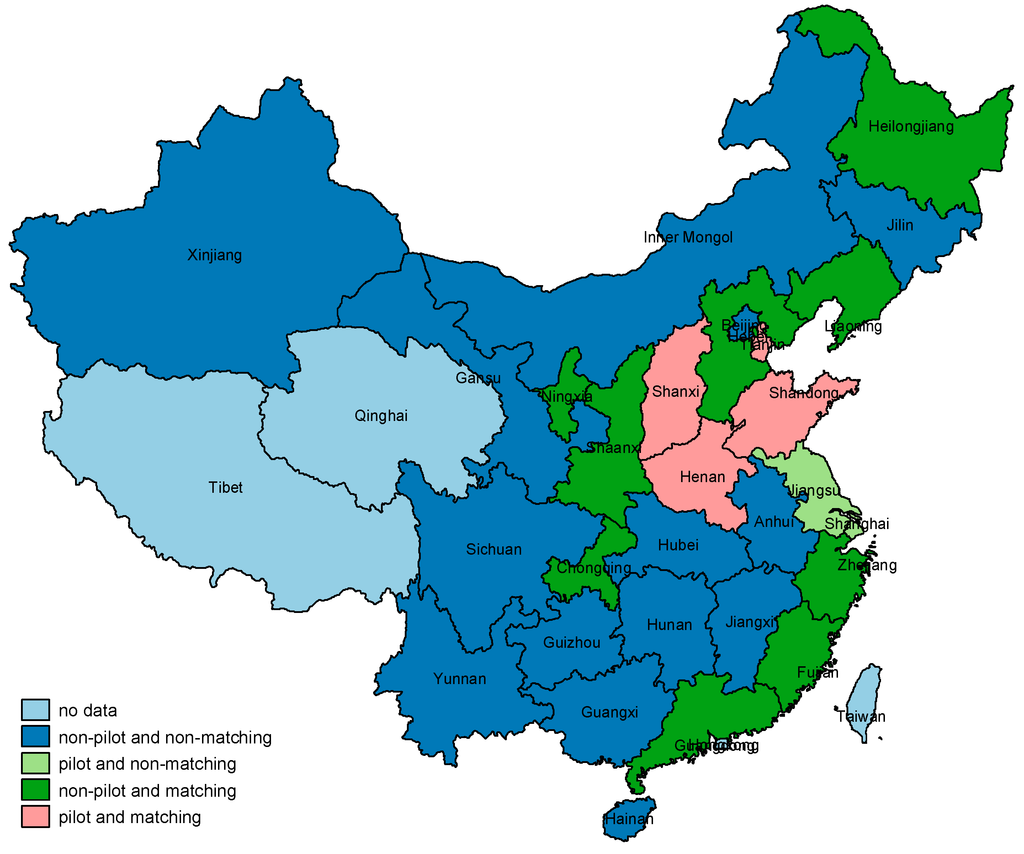
Figure 3. Geographic distribution of matching pilot provinces and non-pilot provinces in 2001.

Figure 3. Geographic distribution of matching pilot provinces and non-pilot provinces in 2001.

As is shown in Table 6, we perform a t-test, which is called the balancing test in this case, on the matching variables between the pilot provinces and non-pilot provinces. It is not difficult to find that each absolute value of difference among matching variables is less than 20, and all of the results of the t-test do not reject the null hypothesis that there is no significant difference among the matching variables between the pilot provinces and non-pilot provinces. In short, the matching results by using the kernel-based propensity score method are proven to be reliable in this paper.

Table 6. Matching balancing test.

Variables	Mean of non-pilot provinces	Mean of pilot provinces	Difference	t-value	Probability
APAC	0.288	0.284	−0.004	0.050	0.959
MPAC	0.935	0.484	−0.451	0.530	0.599
SI	0.027	0.027	0.000	0.100	0.920
EIP	0.943	0.887	−0.055	0.250	0.803
GDPP	0.936	0.983	0.047	0.380	0.703
industrialization	46.019	45.543	−0.476	0.440	0.664
urbanization	42.835	41.823	−1.012	0.210	0.835
state_rate	46.548	46.720	0.172	0.030	0.975

Table 6. Matching balancing test.

Variables	Mean of non-pilot provinces	Mean of pilot provinces	Difference	t-value	Probability
APAC	0.288	0.284	−0.004	0.050	0.959
MPAC	0.935	0.484	−0.451	0.530	0.599
SI	0.027	0.027	0.000	0.100	0.920
EIP	0.943	0.887	−0.055	0.250	0.803
GDPP	0.936	0.983	0.047	0.380	0.703
industrialization	46.019	45.543	−0.476	0.440	0.664
urbanization	42.835	41.823	−1.012	0.210	0.835
state_rate	46.548	46.720	0.172	0.030	0.975

Based on the results of propensity score and matching in the probit model, as shown in Table 7 and Table 8, we can formulate the weighting function by applying the kernel density function and then calculating the effects of SETPS on PAC. This paper regards the dataset of ten pilot years from 2002 to 2011 as a whole sample to obtain the estimates in Table 7, regardless of chronological order. In Table 8, this paper takes chronological order into account and examines the dynamic effects of SETPS on PAC.

Table 7. The effects of SETPS on PAC.

Variables	Non-pilot period (1998–2001)			Pilot period (2002–2011)			Difference-in-difference
	Non-pilot provinces	Pilot provinces	Difference	Non-pilot provinces	Pilot provinces	Difference
APAC	0.288	0.284	−0.004	0.118	0.246	0.127	0.131
	(0.064)	(0.058)	(0.087)	(0.038)	(0.066)	(0.076)	(0.067) *
MPAC	0.935	0.484	−0.451	10.699	3.008	−7.691	−7.240
	(1.001)	(0.435)	(1.092)	(10.581)	(2.838)	(10.955)	(9.932)

Note: Clustered standard errors in parentheses; *** p < 0.01; ** p < 0.05; * p < 0.1.

Table 7. The effects of SETPS on PAC.

Variables	Non-pilot period (1998–2001)			Pilot period (2002–2011)			Difference-in-difference
	Non-pilot provinces	Pilot provinces	Difference	Non-pilot provinces	Pilot provinces	Difference
APAC	0.288	0.284	−0.004	0.118	0.246	0.127	0.131
	(0.064)	(0.058)	(0.087)	(0.038)	(0.066)	(0.076)	(0.067) *
MPAC	0.935	0.484	−0.451	10.699	3.008	−7.691	−7.240
	(1.001)	(0.435)	(1.092)	(10.581)	(2.838)	(10.955)	(9.932)

Note: Clustered standard errors in parentheses; *** p < 0.01; ** p < 0.05; * p < 0.1.

As indicated in Table 7, SETPS has a significant positive effect on APAC, but a negative effect on MPAC, which is not significant. Compared with the mean value in the pilot provinces during the non-pilot period, the APAC in the pilot provinces increased by 45.17% on average, while the MPAC decreased by 2585.7% on average. This shows that SETPS failed to reduce PAC from the past and future perspective. However, this conclusion is based on the dataset of ten pilot years from 2002 to 2011 as a whole sample. Would it be quite different if we investigate the SETPS of each year during the pilot period?

Table 8. The dynamic effects of SETPS on PAC.

Year	APAC		MPAC
	Quantity changes	Percentage changes	Quantity changes	Percentage changes
2002	0.077	26.55	−7.497	−2677.50
	(0.178)		(6.371)
2003	0.161	55.52	–6.051	−2161.07
	(0.267)		(6.709)
2004	0.098	33.79	3.769	1346.07
	(0.120)		(2.623)
2005	0.096	33.10	7.589	2710.36
	(0.109)		(4.995)
2006	0.002	0.69	0.058	20.71
	(0.093)		(0.712)
2007	0.082	28.28	0.435	155.36
	(0.091)		(1.113)
2008	−0.203	−70.00	−42.220	−15,078.57
	(0.191)		(48.084)
2009	−0.486	−167.59	−143.008	−51,074.29
	(0.084) ***		(4.507) ***
2010	−0.031	−10.69	−81.807	−29,216.79
	(0.083)		(50.890)
2011	−0.159	−54.83	−106.000	−37,857.14
	(0.068) ***		(53.962) *

Note: Clustered standard errors in parentheses; *** p < 0.01; ** p < 0.05; * p < 0.1. “Percentage changes” are compared with the mean value in pilot provinces during the non-pilot period.

Table 8. The dynamic effects of SETPS on PAC.

Year	APAC		MPAC
	Quantity changes	Percentage changes	Quantity changes	Percentage changes
2002	0.077	26.55	−7.497	−2677.50
	(0.178)		(6.371)
2003	0.161	55.52	–6.051	−2161.07
	(0.267)		(6.709)
2004	0.098	33.79	3.769	1346.07
	(0.120)		(2.623)
2005	0.096	33.10	7.589	2710.36
	(0.109)		(4.995)
2006	0.002	0.69	0.058	20.71
	(0.093)		(0.712)
2007	0.082	28.28	0.435	155.36
	(0.091)		(1.113)
2008	−0.203	−70.00	−42.220	−15,078.57
	(0.191)		(48.084)
2009	−0.486	−167.59	−143.008	−51,074.29
	(0.084) ***		(4.507) ***
2010	−0.031	−10.69	−81.807	−29,216.79
	(0.083)		(50.890)
2011	−0.159	−54.83	−106.000	−37,857.14
	(0.068) ***		(53.962) *

Note: Clustered standard errors in parentheses; *** p < 0.01; ** p < 0.05; * p < 0.1. “Percentage changes” are compared with the mean value in pilot provinces during the non-pilot period.

As shown in Table 8, the effect of SETPS on APAC showed a general downward trend from 2002 to 2011. SETPS has had a negative effect on APAC since 2008, which reached a peak in 2009 with an APAC reduction of 0.486 (10,000 RMB/ton) and 167.59% in percentage changes. SETPS hardly had a positive effect on APAC before 2008. Such a trend indicates that SETPS has played a certain, but not very outstanding, role in reducing PAC. Meanwhile, the effect of SETPS on MPAC also followed a general downward trend from 2002 to 2011. In the years of 2002 and 2003, SETPS reduced MPAC by 7.497 (10,000 RMB/ton) and 6.051 (10,000 RMB/ton), respectively, up to 2677.50% and 2161.07% in percentage changes. SETPS has been making a positive effect on MPAC since 2004, which once increased by 7.589 (10,000 RMB/ton) and 2710.36% in percentage changes in 2005. After 2008, the effect of SETPS reversed to negative, which reached a bottom in 2009 with −143.008 (10,000 RMB/ton) and −51,074.29% in percentage changes. Such trends are consistent with the conclusion on the mean value comparison between non-pilot and pilot provinces, as shown in Table 2. The APAC and MPAC in the pilot provinces have been constantly lower than non-pilot provinces since 2009. In summary, the year 2009 is a cut-off point for which SETPS began to cause a reduction in PAC.

The previous analyses can lead to the conclusion that the effect of SETPS on MPAC is not significantly negative if we investigate the dataset of ten pilot years from 2002 to 2011 as a whole sample, but the effect is significantly negative in 2009 and 2011 if we investigate each year separately during the pilot period. Meanwhile, the effect of SETPS on APAC was not significantly positive initially, but turned out to be significantly negative in 2009 and 2011. In other words, SETPS began to play a certain role in reducing PAC since 2009. This is in line with the practical experience in other countries that the practical effects of environmental policies needs some time to appear.

6. Conclusions

This paper examines the effects of SETPS on PAC in China during 1998 to 2011. First, this paper calculates MPAC based on the estimated potential output and potential emissions by using network DEA under two different policy scenarios, i.e., command-and-control regulations and standard energy saving and emissions reduction regulations. Then, we analyze the effects of SETPS on APAC and MPAC in the past and future by using the kernel-based propensity score difference-in-difference method. This paper reaches the following conclusions through empirical analysis:

First, SETPS started to show positive effects on reducing PAC since 2009. During 2001 to 2011, SETPS raised APAC by 1,310 RMB per ton on average and reduced MPAC by 72,400 RMB per ton on average, which was not significant. In other words, SETPS failed to reduce PAC as a whole. However, the conclusion would be markedly different if we investigated the effects of SETPS each year of the pilot period separately. SETPS began to show positive effects since 2009 and significantly reduced both APAC and MPAC, especially in 2009 and 2011. Therefore, SETPS began to play an important role in reducing PAC only since 2009.

Second, China, especially non-pilot provinces, should keep putting economic growth in first place because of high PAC. China’s APAC has been fluctuating steadily around the mean value, meanwhile showing a downward trend in recent years. For example, there was a decrease from 0.19 (10,000 RMB/ton) in 2009 to 0.06 (10,000 RMB/ton) in 2010 and 2011. At the same time, China’s MPAC showed an upward trend from 0.29 (10,000 RMB/ton) in 1998 to 9.10 (10,000 RMB/ton) in 2011. This indicates that China is at the stage that it should focus on economic development. Combining the findings on APAC’s and MPAC’s trends, PAC in China, especially in non-pilot provinces, is at the high level. Therefore, China should keep putting economic growth in first place.

Third, the eastern areas should enhance environmental governance, while the central and western areas should encourage economic development. Since these regions are at different stages of environmental governance, the eastern areas rank first in APAC, the central areas follow and western areas lag behind them. However, the conclusion on MPAC is converse. The eastern areas exhibit the lowest MPAC, which indicates that they are at the flat stage. Therefore, the eastern areas should enhance environmental governance; while the central and western areas should encourage economic development, because of their higher MPAC, which indicates that they are at the steep stage.

Based on the above findings, this paper argues that the following counter-measures should be carried out to adjust China’s emissions trading scheme. First of all, China should identify the deficiency of the present emissions trading pilot policies and improve them with respect to their design, as well as their operation. Secondly, China still needs to give priority to economic growth from the perspective of overall economic and environmental development, due to the effects of decreasing APAC and increasing MPAC. Furthermore, China’s PAC has a significant difference among regions. Accordingly, the coordination between economic growth and environment and resources in central and western areas needs to be improved through economic support policies and energy saving technology transfer policies.

7. Limitations and Avenues for Further Investigation

This paper examines the effects of SETPS on PAC by using the kernel-based propensity score difference-in-difference method. Owing to the difficulty in obtaining the official micro-level data in China, we used provincial-level dataset instead in this paper. However, this study paves the way for further research that will be able to obtain a much more reliable estimation with micro-level data. In order to reduce the possibility of unreliable estimation due to the limitation of data, this paper selects a more appropriate estimation method. On the one hand, this paper uses the kernel-based propensity score difference-in-difference method to solve the self-selection problem of the pilot provinces. On the other hand, this paper does a remedial job, such as using four non-pilot years’ data from 1998 to 2001 as a whole sample to estimate the probit model of the propensity score in order to prevent the likely poor results of propensity scores and matching due to the small sample size. In addition, this paper directly uses the difference-in-difference method to estimate Model (9). The results are shown in Appendix

Table A2. The effects of SETPS on PAC based on the difference-in-difference method.

Year	APAC	MPAC
2002−2011	0.246	−5.147
	(0.243)	(8.725)
2002	−0.068	−0.214
	(0.088)	(1.301)
2003	0.030	−2.061
	(0.135)	(2.890)
2004	0.111	−2.852
	(0.215)	(4.592)
2005	0.120	0.271
	(0.215)	(3.152)
2006	0.029	0.054
	(0.225)	(7.110)
2007	0.256	−2.119
	(0.353)	(8.018)
2008	0.137	0.035
	(0.287)	(10.102)
2009	−0.001	−0.264
	(0.338)	(12.107)
2010	0.103	−8.709
	(0.312)	(11.790)
2011	0.100	−9.103
	(0.273)	(13.969)

Note: Clustered standard errors in parentheses; *** p < 0.01; ** p < 0.05; * p < 0.1.

and demonstrate that the kernel-based propensity score difference-in-difference method is reliable in this paper, according to the results of the difference-in-difference method with the same estimated symbol. Nevertheless, the kernel-based propensity score difference-in-difference method is also proven to be a more appropriate estimation method in this paper, because all of the results of the difference-in-difference method are insignificant, due to the self-selection problem.

References

- Coase, R.H. The Problem of Social Cost. J. Law Econ. 1960, 3, 1–44. [Google Scholar] [CrossRef]
- Crocker, T.D. The Structuring of Atmospheric Pollution Control Systems. In The Economics of Air Pollution; Harold, W., Ed.; W.W. Norton: New York, NY, USA, 1966. [Google Scholar]
- Dales, J.H. Pollution, Property and Prices; University Press: Toronto, ON, Canada, 1968. [Google Scholar]
- Montgomery, W.D. Markets in Licenses and Efficient Pollution Control Programs. J. Econ. Theory 1972, 5, 395–418. [Google Scholar] [CrossRef]
- Tietenberg, T.H. Emissions Trading: An Exercise in Reforming Pollution Policy. J. Polit. 1986, 48, 220–222. [Google Scholar] [CrossRef]
- Grubb, M. The Economics of the Kyoto Protocol. World Econ. 2003, 4, 143–189. [Google Scholar]
- Rose, A. Equity Considerations of Trading Carbon Emission Entitlements. In Combating Global Warming: Study on a Global System of Tradable Carbon Emission Entitlements; Barrett, S., Ed.; United Nations: New York, NY, USA, 1992. [Google Scholar]
- Li, Y.; Shen, K. Emission Reduction of China’s Pollution Control Policy—An Empirical Study Based on Provincial Industrial Pollution Data. Manag. World 2008, 7, 8–17. (In Chinese) [Google Scholar]
- Wang, J.; Tu, Z. Emissions Trading: Theory and Practice. Hubei Soc. Sci. 2009, 3, 103–106. (In Chinese) [Google Scholar]
- He, J.; Xiao, B. The Pilot Start-up of the Emissions Trading and the Definition of Market Player. Reform 2010, 1, 155–159. (In Chinese) [Google Scholar]
- Zheng, W. Assessment of Development Trend of Emission Right Trade System under the Background of Low-Carbon Economy. Reform 2010, 4, 104–110. (In Chinese) [Google Scholar]
- Tan, Z.; Chen, D. Regional Carbon Trading Mode and Its Implementation Path. China Soft Sci. Mag. 2012, 4, 76–84. (In Chinese) [Google Scholar]
- Yan, W.; Guo, S. Can Sulfur Dioxide Emissions Trading Policy Reduce Pollution Intensity?—An Empirical Study Based on the Difference in Difference Model. Shanghai J. Econ. 2012, 6, 76–83. (In Chinese) [Google Scholar]
- An, C.; Tang, Y. Research on Decision Model of Enterprises’ Carbon Emission Reduction under Emission Trading System. Econ. Res. J. 2012, 8, 45–58. (In Chinese) [Google Scholar]
- Fan, J.; Zhao, D.; Guo, T. Research on Carbon Emission Trading Mechanism from Consumer Perspective. China Soft Sci. Mag. 2012, 6, 24–32. (In Chinese) [Google Scholar]
- Fan, J.; Zhao, D.; Jin, H. The Effects of Consumption Emissions Trading on Consumer’s Choice—Evidence from Experimental Economics. China Ind. Econ. 2012, 3, 30–42. (In Chinese) [Google Scholar]
- Ferng, J. Allocating the Responsibility of CO2 Over-emissions from the Perspectives of Benefit Principle and Ecological Deficit. Ecol. Econ. 2003, 46, 121–141. [Google Scholar] [CrossRef]
- Cui, L.; Ying, F.; Zhu, L.; Bi, Q.; Zhang, Y. The Cost Saving Effect of Carbon Markets in China for Achieving the Reduction Targets in the “12th Five−Year Plan”. Chin. J. Manag. Sci. 2013, 21, 37–46. (In Chinese) [Google Scholar]
- Li, G.; Ma, Y.; Yao, L. The Intensity and Upgrade Path for China’s Industrial Environmental Regulation—An Empirical Study of the Costs and Benefits of China’s Industrial Environmental Protection. China Ind. Econ. 2010, 3, 31–41. (In Chinese) [Google Scholar]
- Boyd, G.A.; George, T.; Pang, J. Plant Level Productivity, Efficiency, and Environmental Performance of the Container Glass Industry. Environ. Resour. Econ. 2002, 23, 29–43. [Google Scholar] [CrossRef]
- Chen, S. Marginal Abatement Cost and Environmental Tax Reform in China. Soc. Sci. China 2011, 3, 85–100. 222. (In Chinese) [Google Scholar]
- Färe, R.; Grosskopf, S.; Carl, A.P., Jr. Joint Production of Good and Bad Outputs with a Network Application. In Encyclopedia of Energy, Natural Resources and Environmental Economics; Elsevier: San Diego, CA, USA, 2011. [Google Scholar]
- Tu, Z.; Shen, R. Dose Environment Technology Efficiency Measured by Traditional Method Underestimate Environment Governance Efficiency? From the Evidence of China’s Industrial Provincial Panel Data Using Environmental Directional Distance Function Based on the Network DEA Model. Econ. Rev. 2013, 5, 89–99. (In Chinese) [Google Scholar]
- National Bureau of Statistics of China. China Statistical Yearbook 1999–2012; China Statistics Press: Beijing, China, 2013. [Google Scholar]
- National Bureau of Statistics of China. China Energy Statistical Yearbook 1997–2012; China Statistics Press: Beijing, China, 2013. [Google Scholar]
- National Bureau of Statistics of China. China Compendium of Statistics 1949–2008; China Statistics Press: Beijing, China, 2010. [Google Scholar]
- National Bureau of Statistics of China. China Statistical Yearbook on Environment 2012; China Statistics Press: Beijing, China, 2013. [Google Scholar]
- National Bureau of Statistics of China. China Industry Economy Statistical Yearbook 2001–2012; China Statistics Press: Beijing, China, 2013. [Google Scholar]
- Tu, Z.; Shen, R. Industrialization’s, Urbanization’s Dynamic Marginal Carbon Emissions—The Analytical Framework Based on LMDI “Two−Level Perfect Decomposition” Method. China Ind. Econ. 2013, 9, 31–43. (In Chinese) [Google Scholar]
- Tu, Z. The Shadow Price of Industrial SO2 Emission: A New Analytic Framework. China Econ. Q. 2009, 91, 259–282. (In Chinese) [Google Scholar]
© 2014 by the authors; licensee MDPI, Basel, Switzerland. This article is an open access article distributed under the terms and conditions of the Creative Commons Attribution license (http://creativecommons.org/licenses/by/4.0/).