1. Introduction
Urban development with low-density, dispersed, auto-dependent and environmentally and socially impacting characteristics is often referred to as
sprawl [
1]. Communities recognize
sprawl as a concern for many reasons. Local concerns are often placed into the larger context of global trends in urbanization as seen in climate change, water availability [
2] or as some [
3] suggest simply placing in a context of reality to adjust to these changes. Sprawl can increase car use as recognized in Christchurch, New Zealand [
4], it can be a driving force for environmental change in the biosphere [
5], and spatial patterns of urban sprawl are often fragmented [
6] as recognized in the Brussels region in Europe. These spatial patterns of change impact land use which in turn impact the environment. An interesting challenge was raised to ecologists [
7], as well as landscape and urban planners, in how to anticipate social, environmental and economic change and how to manage that change by working with communities to ensure sustainability. Like the definition of sprawl, the causes of sprawl have been debated with some suggesting that developing countries see sprawl as a preference and developed countries see sprawl as a choice [
8]. Whether a choice or preference, sprawl is real and as sprawl moves across the urban continuum from urban to rural fringes, policy makers are becoming increasingly aware of the impacts from sprawl.
These contexts of urban sprawl can be modeled to gain relationship appreciation between
sprawl and landscape change, but how can a community measure this change? Some authors have debated the positive as well as the negative attributes of sprawl [
9,
10]. In Europe it has been measured from a multidimensional perspective [
11], and in Beijing sprawl has been measured using multidimensional indicators [
12], each calculating different sources of data using spatial indices. Can we build on these multidimensional approaches to demonstrate how amount, spatial configuration, and per capita land usage can be measured and combined to form a descriptive amalgamated sprawl index (ASI) to assist policy makers in managing these changes?
Sprawl, is a concern for many stakeholders in the United States of America [
13,
14] and around the world. Sprawl tied with crime as the leading local concern for Americans in a Pew Center poll [
15]. For example, rather than urbanized cities, some [
16] recognized exurban areas as the fastest growing areas. These communities outside of urban areas often do not have the financial/technical resources or political capacity to address this form of urbanization. With relatively recent land conversion rates, America will convert 112 million acres of landscape to urban uses in the next 25 years and another 100 million acres by 2050 [
17]. While China’s government has instituted farmland protection regulation, estimates of total cropland in China for early to mid-1990s range from 125 to 145 million hectares [
18]. The European Environment Agency has reported a loss of agricultural land due to sprawl in the Mediterranean coastal region during the 1990s and most of that was high quality soil for agriculture. Some communities have recognized the metropolitan area development influence on surrounding rural communities and as some [
19] suggest that the landscape is something most people can relate to easily when they see the loss of agricultural land, or other impacts from urban development. Landscape protection becomes a challenge to balance the different interests and values placed on areas of growth around cities. These rural community policy makers understand the importance of measuring sprawl and potentially predicting where it might occur for aesthetic, environmental, logistical, and quality of life, as well as pragmatic financial reasons.
Sprawl has been used to define a variety of conditions, which establish patterns, describe a process or are a result of certain consequences. In The New Global Frontier [
20], a chapter of the book focuses on growth patterns of urban sprawl which are seen as a new challenge to the pressure that comes from the consumption of space in a globalized world. The consumption of open space impacts the environment which suffers from the loss of biodiversity, from accelerating climate change, and from compromising watershed protection. The term
sprawl stems from the conflation of ideology, experience, and effects [
21] and cannot be both a reason and a result. Not only has sprawl been an ambiguous term to define but the scale in which sprawl has been measured tends to focus on the metropolitan or suburban level leaving many areas of the United States and Europe that do not fall in the category of metropolitan or suburb. While U.S. Census data suggest that metropolitan areas are where most growth occurs and will occur, rural areas and states have many counties that do not fit into these definitions of metropolitan areas, and are often underrepresented in sprawl literature and analyses. Some states develop most of the land-use policy at the county level individually that may or may not have land-use decision-making at the metropolitan aggregation. Future projections of land use in Europe suggest that agricultural land has a profound impact on the quality of the landscape and environment, therefore helping to measure landscape change is important for policy makers in these urban continuums [
22].
The purpose of this study was to demonstrate a way to measure urbanization patterns using freely available geospatial data with commonly found analysis software across an urban-rural continuum utilizing established political boundaries. By providing this approach to measuring sprawl to the literature, other regions can add this perspective of how sprawl can be measured and documented in these fringe landscapes. This paper will not argue for or against sprawl and does not attempt to predict sprawl as a cause or effect. Therefore, the paper begins with a review of several sprawl conceptions found in the literature, including geospatial measures to help communicate how sprawl indicators were chosen for this study. This paper supports the literature of defining and measuring urban development patterns by combining amount, spatial configuration, as well as human per capita land usage at the mesoscale with remotely sensed data across the rural-urban continuum through a descriptivenon-parametric multivariate index to support Hasse’s [
1] definition of sprawl characterized by urban development with low-density, that is dispersed, auto-dependent and environmentallyand socially impacting (formating issues).
2. Background: Defining and Measuring Sprawl: What’s Important?
Sprawl has been an elusive term to define and measure [
23,
24]. Sprawl is linked to a plethora of issues including economic [
9,
24], pollution [
25], environment [
26], social capital [
27], transit oriented development [
9], water degradation [
28] and conservation challenges [
29]. The existing literature reveals a variety of spatial and/or non-spatial measures of sprawl from entire Caribbean islands and metropolitan areas to the Census tract scale [
21,
30,
31,
32,
33,
34]. This paper builds on, these approaches and allows for landscape scale comparisons explicitly at a mesoscale utilizing widely available existing classified satellite land use/cover and population data.
Scholars have offered descriptions/definitions of sprawl from Whyte [
35] through more recent conceptions such as Galster
et al. [
21], Clapham [
36], Sutton [
33], Martinuzzi
et al. [
31]. These references are in addition to Ewing’s [
10] widely cited characterization which includes several development types such as: low-density, strip, scattered, and leapfrog. How a person conceptualizes sprawl is an important consideration when measuring. For example, some people may conceptualize sprawl as only an aesthetic condition while other people look to the spatial development form. Sprawl can be conceptualized as relative and transecting across the urban-rural land continuum. The term stems from the conflation of ideology, experience, and effects. When characterizing conditions and traits, sprawl can then be a useful concept describing human settlements occurring in urban or urbanizing areas [
21]. The challenge in addressing sprawl continues to be determining its definition and measurement.
As with other efforts [
10,
21,
33], (Wilson
et al. [
37]), the literature review to determine a common sprawl definition was not entirely conclusive. Some agreement did exist in that sprawl is a relatively wasteful method of urbanization [
34] and is often regarded as a lazy and unrefined urbanization expression [
9]. A strength of one study was its use of a 22 metric model of sprawl to measure 83 metropolitan areas across the nation which included: population, diffusion of homes and workplaces, roads and access, and activity centers [
38]. The metrics were combined into the four dimensions creating an overall Sprawl Index. A unique aspect of the study was measuring sprawl’s impact on quality of life with a key recommendation from this study for taking steps to reduce sprawl and promote smarter growth to improve quality of life. Because this study is not restricted to urban areas, the included rural areas of this study can be associated with other rural areas where policy makers are concerned about encroachment of sprawl from surrounding urban areas. This multidimensional sprawl picture was the first identified during this literature review to analyze related impacts.
There are studies outlining scenarios contributing to sprawl such as rent, demographics, transportation, taxes, and land use regulations [
33,
39]. There are studies that utilize geospatial measures to measure sprawl, in particular, Blankenship [
40] and Clapham’s [
41] use of impervious cover. Another geospatial approach is Irwin’s [
16] statistical model of residential land use pattern change for an exurban area of Cleveland, Ohio, USA. Using land use conversion based on location, a relationship between each land parcel to a series of geospatial variables was developed. The study demonstrated the effectiveness of measuring the rural-urban interface in a spatially explicit manner. One limitation is that the process requires extensive data that may not be readily available in all parts of the country or world.
Galster
et al. [
21] has conducted perhaps the most detailed analysis of sprawl to date according to Song and Knapp [
32]. The Galster
et al. study outlined eight sprawl dimensions: density, continuity, concentration, clustering, centrality, nuclearity, mixed uses, and proximity. Sprawl was defined as low values on one or more of the eight dimensions. Each dimension was defined and tested in multiple urban areas to demonstrate a proof of the concept.
2.1. Urban Rural Continuum: Does Sprawl cross Metropolitan Boundaries?
The literature often keeps the context of sprawl within the metropolitan/urban area with limited examination outside this area [
30,
32,
38,
41,
42,
43]. A reason might be explained by the census (U.S. Census Bureau) reporting over 280 million people living in the United States in the year 2000 with 80% living in metropolitan areas. The remaining 20% of the population lives in non-urban areas, although these areas constitute almost 75% of United States counties. The majority of economic and population growth has occurred in metropolitan regions, mostly in their outer areas [
17]. Looking to the future, conversion of rural lands to urban with an increase in personal income and proximity to existing population centers are predicted to occur [
44].
In relation to agricultural land, the United States Department of Agriculture recognized two kinds of growth: growth at the urban fringe and beyond the urban fringe [
45]. Both affect the amount and productivity of agricultural land and lead to additional opportunities and constraints. Between 1982 and 1997, over half of the newly developed land in the U. S. was converted from farmland and another third from forestland [
46]. Based on landscape pattern metrics, residential development has been shown to account for over 85% of development in the last 30 years, increasingly fragmenting agricultural landscapes [
47]. These fringe areas often extend beyond the metropolitan designated realm into exurban or rural areas.
2.2. Urban Rural Continuum: Does Sprawl cross Census Boundaries?
On the other hand, land use patterns at the census tract scale are important in explaining some aspects of sprawl. The tract scale is a census spatial measure that is larger than neighborhood scale and closer to a community scale of measure. Hasse [
30] provides an approach for measuring geospatial characteristics of development areas for sprawl characteristics. His approach utilized twelve geospatial metrics, such as nearest neighbors, travel time, and impervious surfaces,
etc., to compare location and configuration of three subdivisions. This approach could be used to evaluate and compare other existing developments and development proposals during the site planning review stage. Measuring urban development can also include a regional scale context. A weakness of Hasse’s approach is that it could be especially time consuming if used over regional scales without a high degree of computer automation in image/pattern recognition and analysis.
Through regulations, local government plays an important role in influencing development patterns [
48]. Ulfarsson and Carruthers [
41] recognize how the political and spatial dimensions of metropolitan areas are interconnected. In their study, a five-year interval was used to measure how urban development patterns affected spatial outcomes municipal fragmentation relative to density, spatial urbanized land area extent, property values, and the effect these values have on municipal fragmentation or division. The results indicated that greater municipal fragmentation leads to lower densities, less developed land, and higher property values. Municipal fragmentation also has the potential to push development, a spillover effect, to less regulated areas. The analysis demonstrated the relationship between the built environment, municipal fragmentation and the self-perpetuating effect of a fragmented political landscape. The findings suggest urbanization policies be developed at a larger scale, thus combining these fragmented communities into a larger growth model.
Comparing regions by urban development patterns is important for potentially understanding how different ideologies and policies influence the built form. For example, in the United States, the largest hectare increase in developed land between 1982 and 1997 was in the South [
44]. In addition, the South on average adds more developed area per additional resident. These trends have important implications for land use planning and characterizing urban sprawl and comparing them across the landscape using meso-scaled data is valuable because sprawl is not only found in metropolitan areas, and are also found anywhere growth is occurring
Because sprawl has been studied mostly in urban context and the impact of sprawl is felt beyond the urban continuum, a measure of sprawl is needed that places sprawl indicators into a larger landscape context. Galster’s model is used in a broader landscape to provide policy makers outside of urban areas a means to measure the growth of sprawl. Sprawl is not only for those areas concerned about growth moving away from the center, it is also important for those policy makers to know when it is headed their way. For this reason the measure of sprawl in this study uses county wide measures to help identify where sprawl is impacting the rural landscape.
3. Development Density and Spatial Configuration
Housing density is often cited as an important consideration when characterizing sprawl; however, there is little agreement about what is the appropriate measurement specification [
9]. At what density is development considered sprawl? Scattered development isolates residences and employment opportunities while travel times in sprawled areas typically increase, as do associated environmental damage and energy consumption [
34,
49].
Just as amount or density is often used as sprawl measures, spatial configuration of the development is sometimes included as a measure when characterizing sprawl. Borrowing from landscape ecology methods provides some measurement options. A landscape is a mosaic of habitat patches [
50]. These patches could be habitat for wildlife or they could be human habitat or urbanization. Metrics of landscape pattern attempt to measure two characteristics of the landscape: spatial composition and configuration [
51]. Composition refers to the number and size of different patch types. Configuration refers to the spatial distribution within the landscape. The urbanization scatter pattern becomes apparent in a variety of landscape forms, including leapfrog or discontinuous development [
52]. The results are pieces of urbanized land that sit in isolation from other pieces of urbanized land [
49].
3.1. Study Area
Rural areas might not come to mind as a high growth or sprawling regions; however, this region provides an opportunity to demonstrate an amalgamated index of sprawl across a rural-urban continuum. Kentucky is a state with 120 county governments and numerous smaller geographic jurisdictions making most land use decisions [
53]. Typically, Kentuckians identify home as being at the county scale and many land use decisions are made at the county government level. Therefore, using county geography is important when discussing this region with people. In addition, comparing development patterns across the county helps decision makers recognize that sprawl does not only occur in urban areas and puts his/her county’s patterns in a larger context. By linking the counties into a region, the data can become more useful to policy decision makers in targeting urbanization and its implications to a range of environmental and cultural conditions.
This specific study area was chosen because of the typical characteristics found in growth regions adjacent to metropolitan areas, but also because of some unique designations within this study area. For instance, Lexington-Fayette County has had a defined urban service area since 1958 [
42,
54]. In addition, the study area includes much of the famed “Bluegrass Cultural Landscape” that was placed on the World Monuments Fund 2006 Watch List of the 100 most endangered sites [
55]. One motivation for characterizing urbanization is the inability of many stakeholders (
i.e., policy makers, landowners, developers, and community leaders) to meaningfully quantify and characterize landscape in this way.
The study goal was to create a county level descriptive urban development index using publically available geospatial data that is likely to be available across the United States since [
34] sprawl is about space filling and Ewing [
10] indicates that it is a matter of degree. This study relies on several variables to characterize the multi-dimensional phenomenon as alluded to by previous efforts to measure sprawl [
33]. Multiple metrics based on the amount, spatial configuration, and per capita use of the landscape for urban development were measured and combined to produce an Amalgamated Sprawl Index (ASI).
3.2. Amalgamated Sprawl Index (ASI)
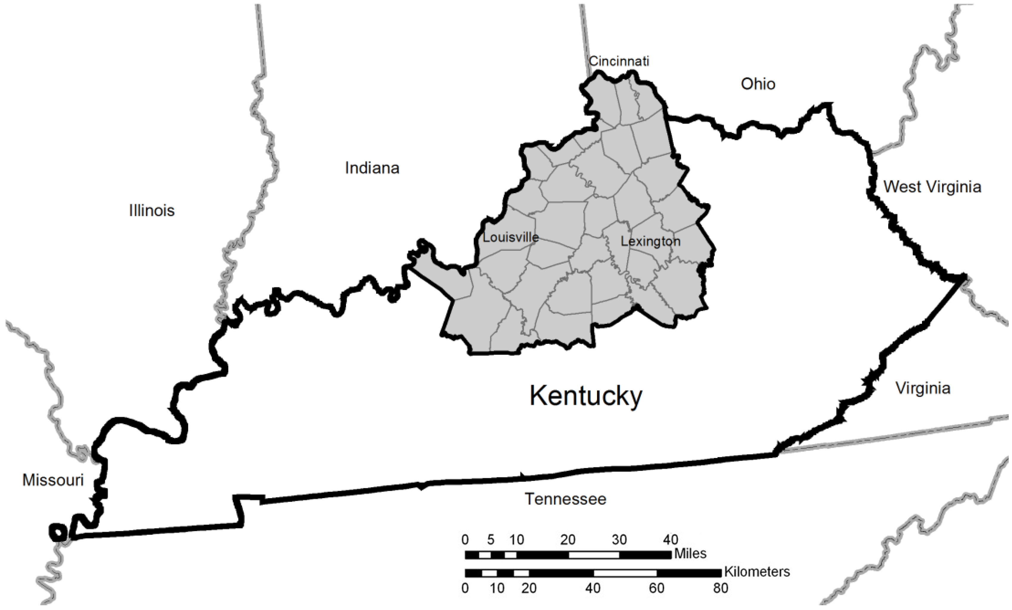
Similar to Ewing’s [
38] sprawl study, demographic data collected from census reports and digital information derived through GIS were tabulated and ranked to form an index. This multi-indicator approach enabled the authors to measure how areas sprawled and to what degree. Some communities recognize the impact to quality of life issues related to sprawl at not only the site scale, but also a larger metropolitan scale. In order to demonstrate the ASI method of sprawl characterization, a 34-county region in north central Kentucky was identified as having exemplar characteristics of development across the urban-rural land continuum. The study area is roughly bounded by Louisville in the west, Lexington in the east and Cincinnati, Ohio, in the north (
Figure 1). One of the important study aspects is that the region encompasses parts of three Metropolitan Statistical Areas (MSA) as well as planning units (counties) not in any MSA. In the Ewing
et al. [
38] study, the Cincinnati, Ohio, Primary Metropolitan Statistical Area (PMSA) was considered just slightly below average in terms of sprawl, ranking 39th out of the 83 areas included in that study.
Figure 1.
This map indicates the area of study in north central Kentucky, USA. The area includes 34 counties which contain some of the fastest growing areas in the region.
Figure 1.
This map indicates the area of study in north central Kentucky, USA. The area includes 34 counties which contain some of the fastest growing areas in the region.
In the current study, the county is the unit of analysis. The county was chosen as the unit because this is the dominant land-use planning jurisdiction within the region. Some study area counties have effectively no land use regulations or review bodies [
56]. Most counties in the study area have experienced human population growth with some counties experiencing almost 50% growth in 11 years (1990–2001) [
57]. The study area counties have a horizontal plane average area of 697 square kilometers [
58] and range in human population from 7,933 to 694,905 people.
3.3. Data and Indicators
The ASI combines readily available demographic data and geospatial data and integrates them within GIS. Data, such as population, development amount and pattern, as well as impervious cover are used in the ASI. Where appropriate, indicators are calculated on a per capita land use basis. The per capita basis allows for more consistent comparisons between counties.
In this study, the raster data used were the 2001 National Land Cover Datasets (NLCD) [
59]. The goal of the NLCD project was to produce a consistent land cover data layer for the conterminous United States using Landsat thematic mapper (TM) data [
60]. As part of the MRLC (Multi-Resolution Land Characteristics) product set, an impervious layer Yang
et al. [
61] was also used in this study. Raster data were processed as an Environmental Systems Research Institute (ESRI) GRID with 30-meter resolution. By combining both geospatial and demographic data, the non-weighted AIS system comprises an overall index with individual measures for characterizing urban development across a region. The ASI is relative only to the counties contained in the study area although the approach could be used across the country.
3.3.1. Indicator Data Utilized
By combining the amount and spatial configuration of urban development with per capita land usage, the data were assembled into a framework of sprawl indicators. A description of how each indicator was measured follows and grouped in categories of amount indicators, spatial configuration indicators, and per capita land usage indicators.
3.3.2. Amount Indicators
Amount variables were chosen to represent physical measurements of urban development in the landscape using 2001 NLCD data and impervious data. The 2001 NLCD data contained classification of urbanized areas in four categories as well as several categories representing forests, agriculture, and water. There have been numerous studies that have defined scenarios that contribute to sprawl such as rent, demographic changes, transportation, tax policies, and land use regulations [
23]. These amount variables help to bring the geospatial context into this study, similar to [
30] multi-indicator approach of sprawl, which help determine how it might occur.
(1)
All Development as of 2001: All development within a county was measured to determine the amount of horizontal space classified as urban development. These areas were identified by reclassifying the four urban classes of the 2001 NLCD data into one urban class while reclassifying all the other classes to a non-urban class. The result is a dichotomous GRID of urban and not urban. Subsequently, the total developed area for each county was calculated. For each county, total land area was determined from the Kentucky Atlas [
58]. A lower county developed percentage developed is considered less sprawling while a county with a higher percentage of the landscape developed is considered more sprawling. Using all development as an indicator helps put this measure into perspective of the spreading out of a community [
62].
(2)
Low Intensity Development as of 2001: Low-intensity development is considered one of the major components of sprawl due to its footprint on the landscape [
29,
63,
64] and this is why it is used here as an indicator. According to the 2001 NLCD metadata, low intensity development is a mixture of constructed materials and vegetation. It is noteworthy for policy makers to be aware of where these developments are occurring in their counties because of their more sprawling character. In this land cover class, impervious surfaces account for 20–49 percent of the land cover and commonly include single-family housing units [
61]. A total area for this low intensity development classification was calculated and then as a percentage was calculated for each county. The lower percentages of low-intensity development were considered less sprawling and the higher percentages were considered more sprawling. The other three classes of development were not considered individually, since the key relationship to sprawl here is considered the “spreading out of limbs” or low intensity development in the way [
62] is inferred.
3.3.3. Spatial Configuration Indictors
Urban geospatial configuration is the second indicator set. For example, a county could have 20% of the landscape considered urbanized (developed). This urbanization could occur in a concentrated area (a single town) or it could occur as more of a quilt worked pattern. A development pattern that is concentrated in an aggregated pattern is considered less sprawling than a quilt worked or disaggregated pattern in this study. In essence, the more “clumpy” the pattern of development, the less sprawling it is considered.
Therefore, a Clumpiness Index is used in this study to address the spatial compactness of urbanization using the NLCD data previously reclassified for the amount indicators (All development, Low-intensity development). The Clumpiness Index was calculated by Fragstats, a spatial pattern analysis program for categorical maps [
65]. Fragstats v.3.3 Build 5 quantifies the spatial configuration of patches (developed areas) within a landscape. Clumpy is calculated from the adjacency land use matrix, which shows the frequency with which different pairs of patch types (including like adjacencies between the same patch types) appear side-by-side in the landscape [
65,
66].
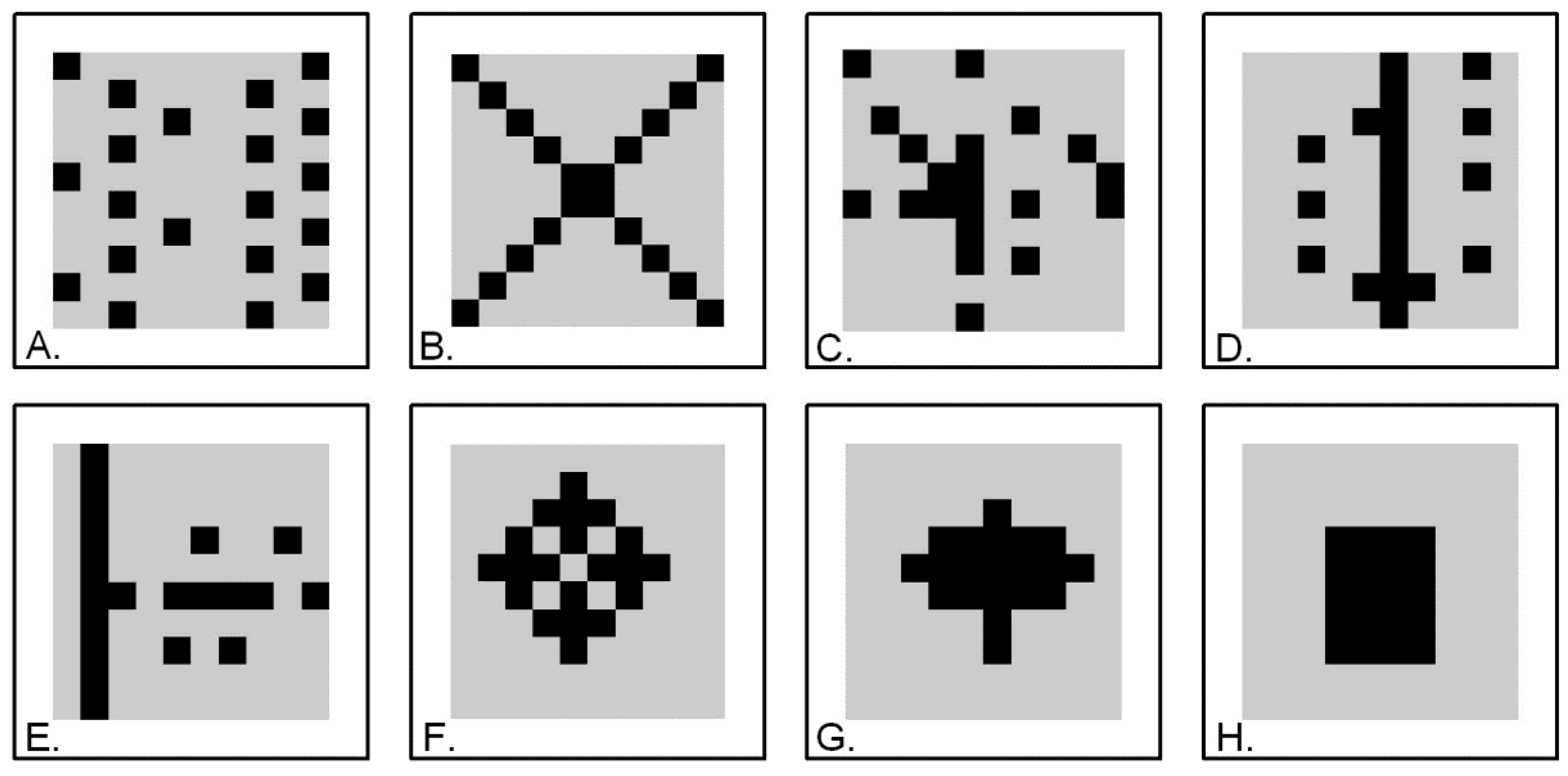
Clumpy equals +1 when attributes are maximally aggregated and −1 when the attributes are maximally disaggregated. Therefore, A higher clumpy score (+1) was considered less sprawling while a lower clumpy score (−1) was considered more sprawling.
Figure 2 has eight example patterns illustrating the Clumpy Index behavior when each hypothetical landscape block is developed at 20%. As the pattern becomes more ‘clumpy’ it becomes less sprawling as depicted in the range of examples A through H with H being most clumpy or least sprawling.
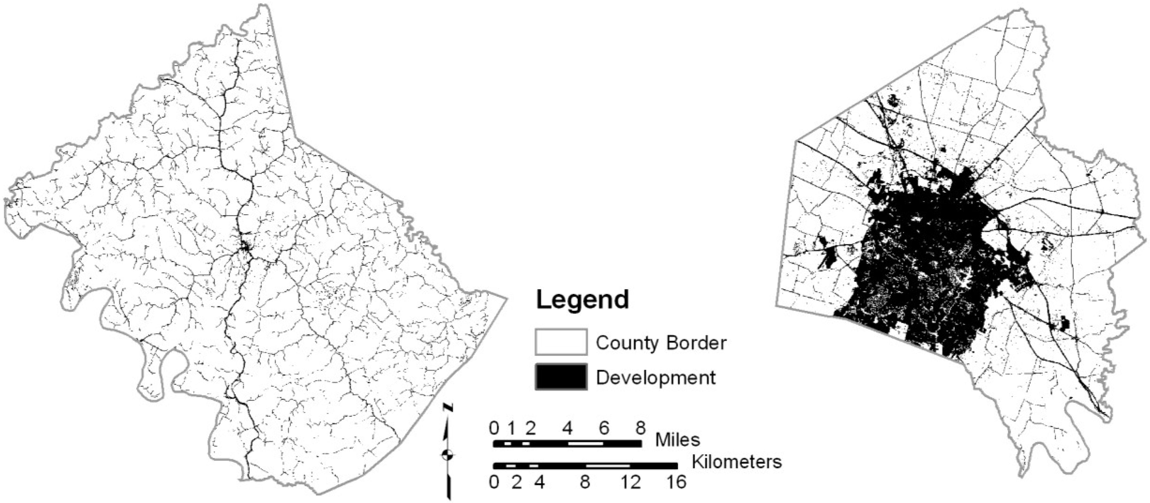
In addition, two figures (
Figure 3 and
Figure 4 below) are shown for visually comparing a more sprawling county (left) with a less sprawling county (right) for the two development classes measured by clumpy in the study area.
(3)
Clumpiness of All Development as of 2001: All development within a county was measured to determine the amount of space within the county that was occupied by development as of 2001 as described in the first amount indicator of this paper. The higher the clumpy index values the lower the indication of sprawl because of the urbanization concentration (
Figure 3).
Figure 2.
These Clumpy diagrams demonstrate a range of density within an area that begins with lower densities (A) and move to higher levels of density found in (H). The more sprawling pattern is seen in (A) with the less sprawling pattern found in (H).
Figure 2.
These Clumpy diagrams demonstrate a range of density within an area that begins with lower densities (A) and move to higher levels of density found in (H). The more sprawling pattern is seen in (A) with the less sprawling pattern found in (H).
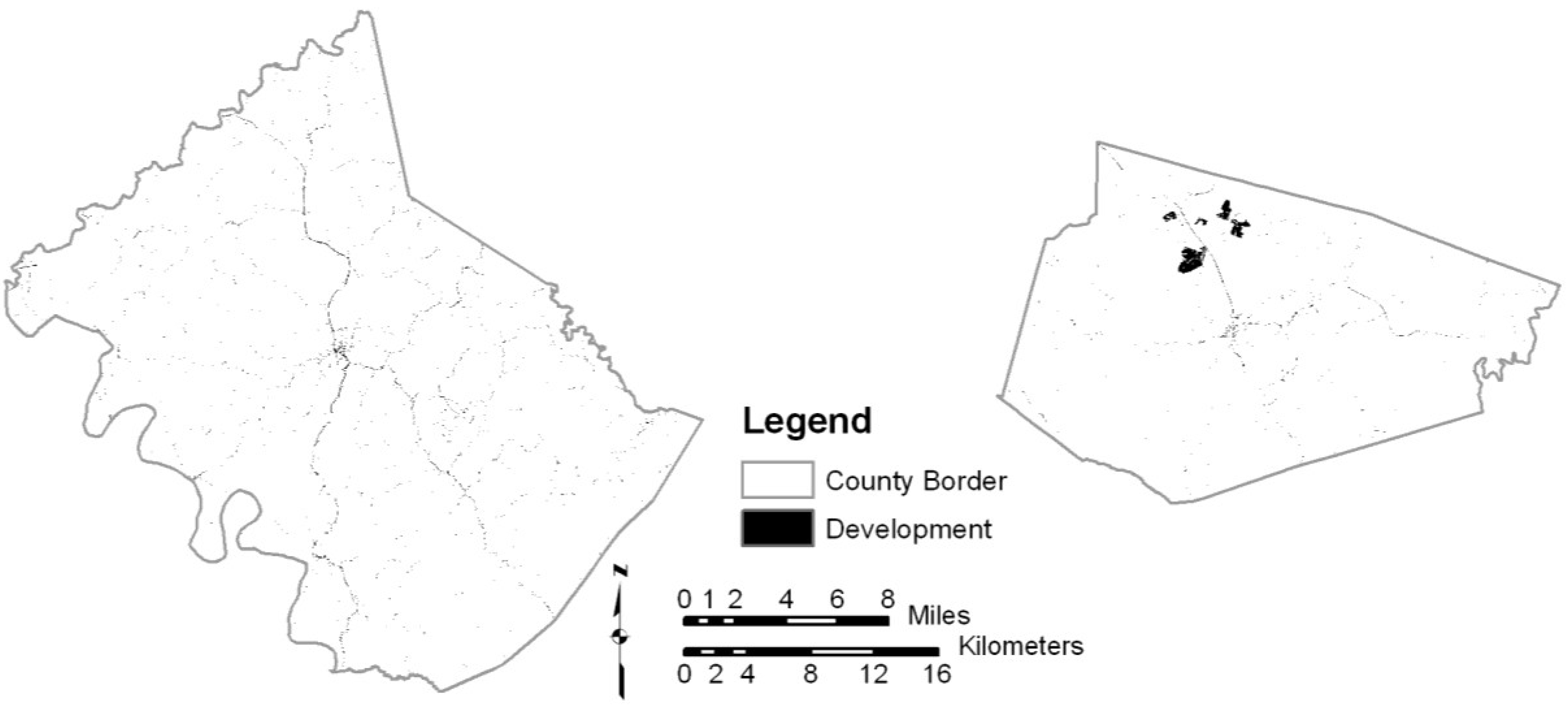
Figure 3.
The two maps indicate a range of county density with one showing more rural character and the other showing a more typical urban or metropolitan pattern. It is important to note that sprawl is not limited to urban areas; growth patterns can take on a sprawling pattern, even in rural areas. Clumpiness helps to define the density of growth.
(4)
Clumpiness of Low-intensity Development in 2001: The 2001 NLCD were reclassified to identify the low-intensity development as described in the second amount indicator of this paper. The higher the clumpy index values the lower the sprawl indication (
Figure 4).
Figure 4.
Even in rural areas, if development is contained in small areas, it defines a less sprawling characteristic.
Figure 4.
Even in rural areas, if development is contained in small areas, it defines a less sprawling characteristic.
3.3.4. Per Capita Land Usage Indictors
Per capita land usage indicators are used to gain a perspective on urbanization at the personal level. For example, if Person A occupies more horizontal space than Person B, Person A is conceptually considered more sprawling. Therefore, in this study, area measures and population (area/population) are used in each of the per capita land usage indicators. It is important that sprawl be seen as something not limited to metro areas, and instead is simply seen as a pattern of density. Even rural areas can have patterns of sprawl.
(5)
2001 Impervious Cover per Capita: Impervious cover has been considered to be a sprawl characteristic [
36,
67]. Total impervious area was calculated on a per county basis and then divided by the number of people living in the county as of 2001 to determine impervious per capita. The population was determined from estimates provided by the Kentucky State Data Center while the NLCD was the source of the impervious cover. Counties with a lower amount of imperviousness per capita were considered less sprawling and counties with higher amounts of imperviousness per capita were considered more sprawling.
(6) Population per Acre (Density): This is a typical density indicator that is often used when describing urban development and was calculated as the number of people per unit area in the county. Higher densities of people per county were considered less sprawling while lower densities were considered more sprawling.
(7) Change in Population Density: The population density change from 1990 to 2001 was calculated for each county. This is used as a temporal component as well as was used to help determine change over time. The counties that increased in density the most were considered less sprawling while counties that increased in density the least (or lost density) were considered more sprawling.
3.4. Amalgamated Sprawl Index Procedures
Conceptually, the ASI approach first measured the spatial amount of urbanization. Second, the ASI used urbanization configuration pattern (Clumpiness). The demographic data (e.g., percent population change, population per acre) are considered the third group of ASI indicators. In total, seven indicator z-scores were combined to produce the descriptive ASI. By not weighting any of the indicators over another indicator, the index then becomes equitable in the distribution of the seven indicators.
3.5. Indicator Standardization
In order to combine indicator variables to form the descriptive ASI, a standardization procedure was necessary. An additional data consideration was required since the data were not normally distributed statistically. Each observation of the seven indicator variables was transformed using a natural log in order to approximate a more normal statistical distribution. After transformation, normality was tested for using the Shapiro-Wilk W test which is typically used for small to medium sized data sets [
68] (
Table 1). Once the data were transformed, a standard score (z score) [
69] was calculated for each observation for each indicator. A z-score is an adjusted score that indicates how many standard deviation units the analogous natural log transformed score is above or below the mean. A z-score of 1 indicates the county on a particular variable is one standard deviation unit above the mean while a −1 indicates a unit below the mean [
70]. A z-score of zero is the mean. This kind of approach is similar to the standardization procedure that was used to map social change by [
71]. The raw scores for the All Development indicator could not be transformed enough to be normally distributed in this study. However, in the end, the transformed indicator was included in the final analysis because of the indicator’s conceptual importance.
Table 1.
The results from testing the raw data for normality before and after natural log transformation. The bold indicates where the natural log did not transform the data enough to be considered normally distributed with the Shapiro-Wilk W test.
Table 1.
The results from testing the raw data for normality before and after natural log transformation. The bold indicates where the natural log did not transform the data enough to be considered normally distributed with the Shapiro-Wilk W test.
| | Before Transformation | After Transformation |
|---|
| Indicator | Shapiro-Wilk (W) | p | Shapiro-Wilk (W) | p |
|---|
| 1. All Development | 0.617 | 0.0001 | 0.857 | 0.0004 |
| 2. Low Intensity Development | 0.602 | 0.0001 | 0.968 | 0.4027 |
| 3. All Development Clumpy | 0.936 | 0.0457 | 0.955 | 0.1732 |
| 4. Low Intensity Development Clumpy | 0.919 | 0.0152 | 0.962 | 0.2801 |
| 5. Impervious Per Capita | 0.923 | 0.0195 | 0.988 | 0.9637 |
| 6. Density Change | 0.749 | 0.0001 | 0.979 | 0.7504 |
| 7. Population Change | 0.899 | 0.0043 | 0.932 | 0.0358 |
3.6. Summing the Indicator Z Scores
In order to create the final ASI, each of the seven indicator z-scores was summed together by county (
Table 2). The individual z-score is relative to the study area mean. Therefore, negative ASI are considered less sprawling than ASI that summed positive relative to the mean. It is important to note that what might be indicated as a sprawling county today could evolve into a compact development in the future as urbanization has been shown to drive building on previously undeveloped sites [
72].
When looking across the entire study area,
Figure 5 indicates where the more sprawling counties are located while
Table 2 contains the individual indicator z-scores as well as the summed z-scores and the resulting sprawl rank. In this study, the least sprawling county was Spencer while the most sprawling county was Bourbon; the average sprawling county was Scott.
Table 2.
The compiled z-scores for each indicator and final amalgamated sprawl index (ASI) (on far right) for each county. A negative score is considered less sprawling while a positive score is more sprawling. The table indicates that Bourbon County has the highest combined rank therefore most sprawling, while Spencer County has the lowest combined rank and therefore least sprawling (both highlighted).
| County Name | All Develop | Low Intensity Develop | Clumpy All Develop | Clumpy Low Intensity Develop | Impervious per capita | Population per acre | Change in Population | AIS Score (Added Z Scores) | AIS Rank |
|---|
| Anderson | −0.606 | −0.325 | 0.098 | 0.215 | −0.145 | −0.300 | −0.836 | −1.898 | 9 |
| Boone | 1.310 | 1.280 | −1.597 | −0.724 | 0.796 | −1.813 | −1.233 | −1.981 | 7 |
| Bourbon | −0.363 | −0.501 | 0.347 | −0.775 | 0.281 | 2.621 | 3.368 | 4.979 | 34 |
| Boyle | 0.066 | 0.033 | −0.511 | −0.049 | 0.004 | 0.429 | 0.694 | 0.666 | 21 |
| Bullitt | 0.190 | 0.855 | −1.532 | −1.986 | −1.178 | −0.940 | −0.660 | −5.251 | 2 |
| Campbell | 1.522 | 1.306 | −0.457 | −0.301 | −0.580 | −0.520 | 1.063 | 2.032 | 27 |
| Carroll | 0.053 | 0.315 | −0.082 | 0.105 | 2.401 | 0.831 | 0.538 | 4.161 | 31 |
| Clark | 0.280 | 0.579 | −0.493 | −0.846 | 0.898 | 0.104 | 0.234 | 0.756 | 22 |
| Fayette | 2.031 | 1.909 | −2.204 | −0.989 | −0.489 | −1.801 | −0.012 | −1.553 | 10 |
| Franklin | 0.787 | 0.870 | −0.842 | −0.605 | 0.416 | −0.140 | 0.581 | 1.067 | 24 |
| Gallatin | −0.212 | 0.018 | 0.237 | 1.001 | 1.376 | −0.347 | −1.157 | 0.916 | 23 |
| Garrard | −0.619 | −1.148 | 1.266 | 1.369 | −0.773 | 0.105 | −0.623 | −0.422 | 15 |
| Grant | −0.572 | −0.184 | 0.545 | 0.342 | 0.087 | −0.435 | −1.068 | −1.286 | 12 |
| Hardin | −0.111 | 0.157 | −0.771 | −0.299 | −0.191 | 0.525 | 1.088 | 0.399 | 19 |
| Harrison | −0.451 | −0.596 | 0.961 | 1.070 | 0.537 | 0.987 | 0.390 | 2.898 | 30 |
| Henry | −0.699 | −0.671 | 1.130 | 0.974 | 0.545 | 0.672 | −0.130 | 1.820 | 26 |
| Jefferson | 3.101 | 2.566 | −2.036 | −0.903 | −0.412 | −1.336 | 1.352 | 2.332 | 28 |
| Jessamine | 0.352 | 0.390 | −0.598 | −0.715 | −0.531 | −1.007 | −0.631 | −2.740 | 4 |
| Kenton | 1.997 | 1.818 | −1.543 | −0.877 | −1.062 | −1.111 | 0.894 | 0.116 | 18 |
| Larue | −0.831 | −1.513 | 0.865 | 0.287 | −0.998 | 0.888 | 0.065 | −1.237 | 13 |
| Madison | 0.424 | 0.591 | −0.405 | −0.743 | 0.482 | −0.588 | −0.435 | −0.674 | 14 |
| Marion | −1.046 | −1.041 | 0.591 | 0.606 | 0.065 | 1.068 | 0.420 | 0.663 | 20 |
| Meade | −1.004 | −1.128 | 1.309 | 0.332 | −1.969 | 0.592 | 0.570 | −1.298 | 11 |
| Mercer | −0.535 | −0.598 | 0.275 | 0.454 | 0.167 | 0.807 | 0.606 | 1.177 | 25 |
| Nelson | −0.758 | −0.576 | 0.211 | 0.331 | −0.456 | −0.139 | −0.560 | −1.945 | 8 |
| Oldham | 0.211 | 0.188 | 0.110 | 0.181 | −1.974 | −1.337 | −1.132 | −3.752 | 3 |
| Owen | −0.753 | −0.834 | 1.504 | 1.664 | 1.775 | 1.138 | −0.086 | 4.406 | 32 |
| Pendleton | −0.613 | −0.865 | 1.371 | 1.664 | 0.546 | 0.558 | −0.252 | 2.410 | 29 |
| Scott | 0.347 | 0.333 | −0.146 | −0.234 | 1.350 | −0.680 | −0.971 | −0.001 | 17 |
| Shelby | −0.609 | −0.158 | −0.365 | −0.457 | 0.370 | −0.299 | −0.847 | −2.366 | 5 |
| Spencer | −0.988 | −0.306 | 0.737 | −2.641 | −1.150 | −0.556 | −1.649 | −6.554 | 1 |
| Trimble | −1.072 | −1.710 | 1.009 | 1.645 | −1.221 | 0.091 | −0.820 | −2.078 | 6 |
| Washington | −0.979 | −1.092 | 1.042 | 1.193 | 1.175 | 1.959 | 1.295 | 4.594 | 33 |
| Woodford | 0.149 | 0.034 | −0.026 | −0.287 | −0.142 | −0.026 | −0.059 | −0.357 | 16 |
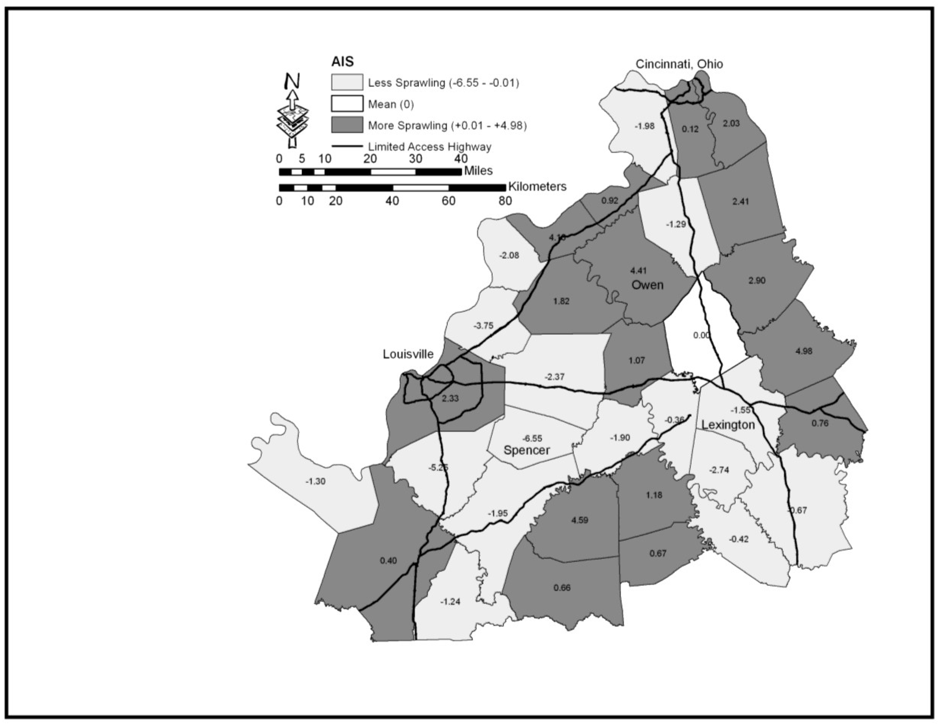
Figure 5.
The darker areas indicate the more sprawling characters when using the ASI, while the lighter areas indicate a less sprawling character.
Figure 5.
The darker areas indicate the more sprawling characters when using the ASI, while the lighter areas indicate a less sprawling character.
4. Findings: Sprawl Increasing or Decreasing?
It is important to be reminded that the roughly triangular study area is anchored by three major population areas of Kentucky (Louisville to the west, Lexington to the south, and Cincinnati to the north) while simultaneously the study area also contains some of the least populated counties of the state (
Figure 5). This approach attempted to span across the urban-rural continuum and not focus analysis only on metropolitan areas as other studies have done. As the sprawl indicators were compiled using standardized z-scores, the results communicated an interesting results set. While sprawl has been measured in this region, it is not necessarily seen as a rapid measure, but sprawl is not necessarily defined by the pace of change, and instead is simply recognized as a density of change. The results depict that sprawl in the study area is found to have more of an extreme that is less sprawling, than the more sprawling extreme.
Spencer County had an ASI score of −6.554 (less sprawling) and Bourbon County had an ASI score of +4.979 (more sprawling), while Scott County had essentially the mean ASI score (−0.001) (
Table 1). None of the counties scored at opposite extremes in any combination of indicators, meaning it was both the least sprawling in one indicator but most sprawling in another; however, some counties did score at extremes in more than one indicator. Fayette County has had a growth boundary in place for more than 50 years but it was not the least sprawling county (Fayette County ASI score −1.553). However, Fayette County did score least sprawling in the Clumpy Index of All Development with a z-score of −2.204. The indicator with the most range from high to low was ‘Change in Population’ which measured as high as +3.648 in one county and low as −1.649 in another county for a difference of 5.017 points, and the indicator with the least amount of difference was Clumpy All Development which had a difference in high and low values of 3.708 points.
4.1. Compiling the Data
Compiling the data suggests that sprawl is occurring over the 34 county area to a “lesser degree” than at a higher degree as depicted with the lowest negative score (−6.554) as opposed to the highest positive score (+4.979). Remember the z-scores that are negative indicate less sprawling while positive z-scores as most sprawling in the 34 county study area. In looking at the indicators, Spencer County actually scored the lowest of the 34 counties in two indicators, Clumpy Low Impact Development, and Change in Population Density, and it was in the “lesser” category in six out of the seven indicators, helping it to compile the lowest aggregate score. While Bourbon County had the highest aggregate score of +4.979 (ranked 34 or most sprawling), it also was most sprawling in two of the indicators: Population Density and Change in Population Density. What is interesting here is that Bourbon County only scored in a positive range in four out of the seven categories which once again justifies why these indicators are not ranked. The level of sprawl for any one indicator can impact the aggregate score when all indicators are compared. Is there value to give weight to any indicator or combination of indicators? While these indicators were not weighted, how might one begin to weight any category differently if they were to view the global impact on resources as asked by [
3]. Should one consider amount of imperviousness more highly as it relates to clean water? So, one limitation or strengthen of this approach, depending on perspective, is where a county measured in any one of the indicators can become a driver in the ASI depending on the study area used. Therefore, indicators that encompass a multi-metric approach using publically available data and software is a study strength overall. Fayette County was not the least sprawling, yet has enacted an urban service boundary for over 50 years. The surrounding counties range in sprawl with one adjoining county in the “less sprawling” category, three adjoining counties in the “mean” level of sprawl, and two counties in the “more sprawling” category. Does this suggest that leap-frogging occurs sometimes, but not others? Multiple indicators help to generate a broader understanding of sprawl; yet, the devil is still in the details. The authors chose to initially limit the amount of indicators to simply test the method and add the ASI approach to the sprawl measure discussion while recognizing other indicators could be included.
Population Change was seen to have the widest range in extreme as a category and an interesting correlation was noticed, this measure also paralleled with the overall ranking of sprawl. Bourbon County had the highest level of population change and also had the highest aggregate z-score, while Spenser County had the lowest level of population change and also had the lowest aggregate z-score. Does this mean that population change is a strong indicator of sprawl as suggested by Hasse and Lanthrop [
46]. In this case, there appears to be a connection to population change and sprawl. Related to this, how does overall population impact sprawl? Jefferson County (city of Louisville) is the most populated county in study area [
73] and ranked as one of the most sprawling with an overall rank of 28 out of 34 (most sprawling). Fayette County, one of the other population center counties, ranked 10 of 34 in sprawl. One might recognize the urban service boundary enacted in Fayette County as a deterrent to sprawl, since Jefferson County does not have an urban service boundary. This is a subjective view but these types of observations reinforce how a multi-indicator approach that include spatial measures and per capita measures can help to describe conditions especially for discussion purposes.
The results also suggest that sprawl may not be occurring where one might think it is in the landscape. For example, it might be suggested that where the county population is higher there would be more sprawling conditions which was not always the case in this study. As one reviews the study area (
Figure 5) and its depiction of sprawl by county extent, the relationship to transportation impacts might be of particular interest as suggested by Ewing
et al. [
38]. In addition, sprawl was not necessarily found within the outer reaches of metropolitan areas as suggested by Carbonell and Yaro [
17]. In contrast, what is the relationship between impervious per capita and population increase as questioned by Jat
et al. [
74] Therefore, this approach of using multiple indicators is an advantage in this case because it takes these different sprawl conceptualization situations into account. By not weighting these indicators, an objective index is compiled.
This study area includes some zoning regulations that limit growth due to “growth boundary regulations” which require specific densities of development. This provides dense growth in some of these more populated counties, which provide a more clumpy or dense area of development. This character is less sprawling; however, many counties do not have these growth boundaries and allow sprawl development, which are indicated by their clumpiness scores.
4.2. Lessons Learned
This study used seven sprawl indicators to form descriptive ASI across the urban-rural continuum similar to other studies [
21,
38]. The strength of this approach is that it uses publically available geospatial and tabular data, and commonly available GIS software and the freely available Fragstats analysis software. The approach demonstrated in this study brings indicators to the per capita landscape usage level for imperviousness, which is an important ecological quality indicator [
75,
76]. Building on Crawford’s trajectories [
77] of residential development, a temporal component was initially discussed; however, since there has not yet been a public accuracy assessment for the 2006 National Land Cover Data, there could be a mismatch between the most recent National Land Cover Data and the 2010 U.S. Census data. A temporal component is something the authors would like to utilize into the study once an accuracy assessment is published.
The ASI approach could be applied at almost any geographic unit of analysis depending on the resolution of the land cover/land use data and human population. Just as Frenkel [
78] and Schwarz [
79] have done, sprawl can be measured in Europe as well. For example, the approach could be applied using watershed boundaries [
36] or any of the commonly used census boundaries. The non-weighting of the indicators helps to provide a simple way of measurement for the amalgamated index. While there was no explicit indicator weighting, the choice of indicators in and of themselves drive the overall ASI in the current form and do not focus on either rural or metropolitan areas, but instead go across the urban-rural continuum.
A conceptual range of indicators in the current sprawl literature was used to develop a descriptive index that could be applied to publically available data and software that most government levels have access. The method can be adjusted to include more/less indicators, or different combinations, but similarly as Jaeger
et al. [
80] it is recommended that a both spatial pattern and per capita data be represented to develop an amalgamated index of sprawl.
5. Discussion
Using ASI is a useful approach to help rural stakeholders visualize urbanization patterns on a landscape scale while tying those patterns back to a unit area they are more likely to have identity with (sense of place) and/or land use decision-making power. This research demonstrates how to measure sprawl at the county scale utilizing readily available data and software. The current literature focuses sprawl studies on metropolitan areas, and sprawl is not limited to metropolitan areas. Many rural areas can also have patterns of sprawl, and the sooner policy makers can recognize sprawl indictors, the more they can plan for encouraging or discouraging sprawl.
The study also combines geospatial data as well as per capita land usage to generate the ASI for a multi-indicator approach. The example study area confirmed the utility of this mesoscale sprawl characterization. It is important that rural areas can recognize the density of growth, and by utilizing per capita indicators, policy makers can trend growth areas and the demographics associated with that growth.
A single development, without a regional context, may not appear to be sprawl so there is no perceived issue to address for a community. Therefore, proactive land use planning is critical in the context of describing regional development patterns [
36]. Understanding how a particular development affects the overall regional development pattern has important implications, particularly for policy makers. These patterns of growth can be measured and compared to temporal indicators that will allow policy makers in these rural areas to begin to recognize sprawl patterns and plan for them. If sprawl is conceptualized in a relative sense, then using amount, spatial configuration, and per capita land usage indicators in an Amalgamated Sprawl Index approach is helpful for visualizing a commonly used term that has been historically difficult to apply descriptive measures from metropolitan to rural areas. As planners and policy makers become more aware of ecological impacts to sprawl, these communities with limited resources need methods to predict where sprawl may occur as they plan for more sustainable measures to design for this growth.
6. Conclusions
Policy makers are becoming increasingly aware of the impacts from sprawl as it moves across the urban continuum. While U.S. Census data suggest that metropolitan areas are where most growth occurs and will occur, rural areas and states have many counties that do not fit into these definitions of metropolitan areas, and are often underrepresented in sprawl literature and analyses. It can cost communities financial/technical resources to plan and address sprawl, and often these surrounding rural areas do not have these resources. These rural community policy makers understand the importance of measuring sprawl and potentially predicting where it might occur for aesthetic, environmental, logistical, and quality of life, as well as pragmatic financial reasons. The purpose of this study was to demonstrate a way to measure urbanization patterns using freely available geospatial data with commonly found analysis software across an urban-rural continuum utilizing established political boundaries.
Looking to the future, conversion of rural lands to urban are predicted to occur. Municipal fragmentation also has the potential to push development, a spillover effect, to less regulated areas. A measure of sprawl is needed that places sprawl indicators into a larger landscape context, and the measure of sprawl in this study uses county wide measures to help identify where sprawl is impacting the rural landscape. Just as amount or density is often used as sprawl measures, spatial configuration of the development is sometimes included as a measure when characterizing sprawl. The study goal was to create a county level descriptive urban development index using publically available geospatial data that is likely to be available across the United States since sprawl is about space filling.
Similar to Ewing’s sprawl study, demographic data collected from census reports and digital information derived through GIS were tabulated and ranked to form an index. This multi-indicator approach enabled the authors to measure how areas sprawled and to what degree. The ASI combines readily available demographic data and geospatial data and integrates them within GIS. Where appropriate, indicators are calculated on a per capita land use basis allowing for more consistent comparisons between counties. The ASI approach could be applied at almost any geographic unit of analysis depending on the resolution of the land cover/land use data and human population. Using ASI is a useful approach to help rural stakeholders visualize urbanization patterns on a landscape scale while tying those patterns back to a unit area they are more likely to have identity with (sense of place) and/or land use decision-making power.


