1. Introduction
Day visits constitute one of the most significant of all leisure activities. Just within England the latest estimates suggested that there are currently around 900 million tourism day visits made each year generating over £37 billion of tourism spending [
1]. This clearly reflects a substantial demand for the recreational services of the countryside which is second only to towns and cities as a day visit destination. However, while there is considerable attention paid to the overall level of such demand, research into the drivers of the precise pattern of visits and why some resources attract greater numbers of visits than others is, we argue, less complete. In particular we highlight the failure of previous studies to fully incorporate the spatial context of recreational resources within demand modeling. This paper sets out to extend existing methodologies so as to address these deficiencies.
In modeling demand for outdoor recreation the key methodology is the travel cost approach [
2]. This proposes that the number and value of visits made to any given recreational site should be a function of the travel time and associated costs which an individual faces in visiting it; their income and other socio-economic and demographic factors; the facilities and their quality offered at the site; and location factors including the substitute sites available to the individual. Given this then, ceteris paribus, demand for outdoor recreation sites should be linked to the costs of visiting those sites which, under certain assumptions [
3], allows us to infer the value of those visits. While this method was first suggested over 60 years ago [
4] and has been growing in use since the seminal work of Clawson and Knetsch [
5], it has been dominated by studies which focus upon variables describing on-site facilities and the characteristics of those interviewed
via on-site surveys. For instance, Scarpa
et al. show that both subjective and objective forest attributes, such as recreational facilities, type of coverage and size of trees, are important drivers of individuals’ Willingness To Pay (WTP) for forests [
6]. WTP is the maximum amount a person would be willing to pay, sacrifice or exchange for a good, and the value can be estimated using several methodologies. Scarpa
et al.’s estimation of the mean WTP for single forests is based on a value function that only includes forest and individual characteristics, but fails to account, however, for off-site characteristics. As in most other Contingent Valuation studies, the effect of the availability, distribution and accessibility of substitute sites is completely ignored. This causes two problems: (i) studies have generally failed to include objective measures of substitute availability thus risking the biasing of demand and valuation estimates; and (ii) reliance upon on-site and survey derived respondent characteristics limits the transferability for which generally available secondary source data is preferable. A lack of transferability necessitates that new surveys be undertaken for each policy decision.
The issue of transferability has become of central academic and policy interest in recent years [
6,
7,
8,
9,
10,
11] with the realization that resource constraints limit decision makers’ ability to commission new studies. However, most of the benefits transfer literature has focused almost exclusively upon the estimation of marginal (per visit) values at the expense of assessing the number of visits to which such values should be applied. As we have shown within another context (single site contingent valuation studies [
12]), this strategy raises the prospect of major error as it is the number of visits rather than their marginal value which is liable to be the principal driver of the aggregate value of site creation or improvement.
The present paper focuses upon three issues vital to the successful transfer of recreation studies:
- (i)
We switch the research focus from the estimation of marginal values to the assessment of the quantity demand for visits, thus addressing a major driver of error in assessments of aggregate recreation value;
- (ii)
Although we use survey data to develop our models of recreation demand, we only use predictor variables which are readily available as national coverages of secondary data (e.g., digital map and census derived measures). This substantially enhances the transferability of findings to previously un-surveyed locations;
- (iii)
We use a geographical information system (GIS) to derive further explanatory variables, parameterizing the influence of the location of recreational sites upon demand by introducing new measures of demand drivers such as the spatial distribution of substitutes.
These study aims are addressed through a case study of a typical day-visit recreational resource; multi-purposes, open-access woodland in the UK. We use what is, to our knowledge, the largest survey ever employed for recreational demand modeling, comprising more than 10,000 interviews with day visitors to Forestry Commission woodlands all over Great Britain. Furthermore we employ multilevel modeling techniques to address the inherently clustered nature of data collected from surveys at multiple sites. We also make novel use of detailed GIS environmental characterizations to determine travel costs, the characteristics of outset areas, and the availability and type of substitutes. The practical and theoretical benefits of the approach adopted are discussed.
2. Methodology
The empirical focus of this research concerns the estimation of recreational visitor numbers at a sample of Forestry Commission woodlands across Great Britain. The Forestry Commission is the largest land manager in Britain and the biggest provider of outdoor recreation, being the government agency responsible for the protection and expansion of more than 750,000 hectares of Britain’s forests and woodlands [
13]. Recreational use is a significant aspect of woodland management; 77% of all adults reported visiting woodlands in 2009 [
13]. In addition, woodlands facilitate a wide range of recreational pursuits including walking, cycling, horse riding, orienteering, camping, fishing and bird watching. Public forests also provide a range of key facilities including picnic sites, camping sites, holiday cabins, marked trails, cycle ways, horse riding routes, and information centers.
Development of our empirical demand model draws upon responses from the 1996, 1997 and 1998 Forestry Commission visitor surveys conducted at 40 forest sites across Great Britain. Each site had one interviewer, who interviewed on a continuous survey basis such that when one interview was completed the next individual passing was then interviewed. For groups of two or more people, one person was selected to be interviewed. A count of individuals or groups not interviewed during the survey period was recorded by the interviewer.
Table 1 lists the sites for which survey information was provided and the number of interviews conducted at each. This number is subdivided into day-trippers and holidaymakers, based upon individuals’ responses.
The survey effort expended at each site as measured by survey hours is an important determinant of the number of interviews completed. Therefore, the number of interviews at a site was divided by the amount of survey effort at the site and standardized to a period of a 24 hour day.
Table 1.
Site names, Forest District, numbers of visitors surveyed by type, and survey effort.
Table 1.
Site names, Forest District, numbers of visitors surveyed by type, and survey effort.
| Site Number | Site Name | Forest District | Numbers of Visitor Surveyed | Survey Effort
(Hours) |
|---|
| Total Visitors | Day Visitors | Holiday Visitors |
|---|
| 3 | Afan Argoed | Coed y Cymoed, Wales | 458 | 381 | 76 | 157.0 |
| 6 | Alice Holt | South East England | 217 | 209 | 6 | 82.0 |
| 8 | Back O Bennachie | Buchan, Scotland | 100 | 92 | 8 | 69.0 |
| 9 | Beechenhurst | Forest of Dean, England | 128 | 84 | 43 | 34.0 |
| 14 | Black Rocks | Sherwood and Lincolnshire, England | 161 | 123 | 38 | 72.0 |
| 15 | Blackwater | New Forest, England | 179 | 82 | 93 | 35.0 |
| 17 | Blidworth Woods | Sherwood and Lincolnshire, England | 216 | 211 | 2 | 106.0 |
| 18 | Bolderwood | New Forest, England | 343 | 148 | 194 | 58.0 |
| 20 | Bourne Wood | Northants, England | 211 | 200 | 11 | 59.5 |
| 33 | Chopwell | Kielder, England | 125 | 123 | 2 | 31.0 |
| 34 | Christchurch | Forest of Dean, England | 132 | 26 | 104 | 24.0 |
| 40 | Countesswells | Kincardine, Scotland | 212 | 209 | 3 | 64.0 |
| 43 | Cycle Centre | Forest of Dean, England | 222 | 154 | 67 | 88.0 |
| 44 | Dalby | North York Moors, England | 305 | 157 | 148 | 72.0 |
| 46 | Delamere | West Midlands, England | 684 | 264 | 6 | 153.0 |
| 49 | Dibden | New Forest, England | 215 | 206 | 9 | 89.0 |
| 51 | Donview | Buchan, Scotland | 144 | 126 | 18 | 66.0 |
| 61 | Garwnant | Coed y Cymoed, Wales | 358 | 274 | 83 | 80.5 |
| 66 | Glentrool | Newton Steward, Scotland | 321 | 114 | 205 | 100.0 |
| 68 | Grizedale | Lakes, England | 265 | 68 | 197 | 51.0 |
| 72 | Hamsterley | Kielder, England | 160 | 119 | 40 | 52.0 |
| 80 | Kielder | Kielder, England | 104 | 38 | 64 | 26.5 |
| 83 | Kings Wood | South East England | 102 | 95 | 7 | 72.0 |
| 84 | Kirkhill | Kincardine, Scotland | 207 | 197 | 10 | 107.0 |
| 86 | Kylerhea | Fort Augustus, Scotland | 210 | 9 | 200 | 95.0 |
| 95 | Mabie | AE, Scotland | 686 | 355 | 315 | 108.0 |
| 111 | Queens View | Tay, Scotland | 270 | 41 | 228 | 96.0 |
| 117 | Salcey | Northants, England | 196 | 185 | 9 | 54.0 |
| 119 | Sherwood Pines | Sherwood and Lincolnshire, England | 680 | 517 | 163 | 208.5 |
| 121 | Simonside Hills | Kielder, England | 136 | 98 | 37 | 45.5 |
| 126 | Symonds Yat | Forest of Dean, England | 255 | 103 | 152 | 66.0 |
| 128 | Thetford High Lodge | East Anglia, England | 687 | 535 | 149 | 148.5 |
| 129 | Thieves Wood | Sherwood, England | 307 | 304 | 2 | 108.0 |
| 130 | Thrunton Woods | Kielder, England | 142 | 89 | 52 | 48.0 |
| 134 | Tyrebagger | Kincardine, Scotland | 149 | 139 | 9 | 71.0 |
| 137 | Waters Copse | New Forest, England | 172 | 75 | 97 | 86.5 |
| 141 | Wendover | South East England | 117 | 112 | 5 | 42.0 |
| 143 | Westonbirt Ab | Westonburt Arboretum, England | 440 | 349 | 86 | 44.5 |
| 147 | Willingham Woods | Sherwood and Lincolnshire, England | 176 | 163 | 12 | 124.0 |
| 153 | Wyre | West Midlands, England | 670 | 567 | 101 | 130.5 |
Although the sample of visitors included both day visitors and holiday makers, unfortunately there was no information available for holidaymakers on their place of stay during their holiday. Hence it was necessary to define outset locations as the home location rather than any temporary address (e.g., a holiday residence). Nevertheless, tests were made to determine if any significant bias was associated with this assignation by stratifying the sample into holidaymakers and day-trippers and undertaking separate analyses for each (results not shown here for brevity). The results obtained were generally comparable; unsurprisingly travel time to substitutes was somewhat more important for day visitors as were the demographic characteristics of the outset location. However, the models did not fundamentally differ in either the type of variables included or the strength of effect, and hence we conclude that the models developed here have general applicability regardless of visitor type.
2.1. Environmental and Socio-Demographic Characterization
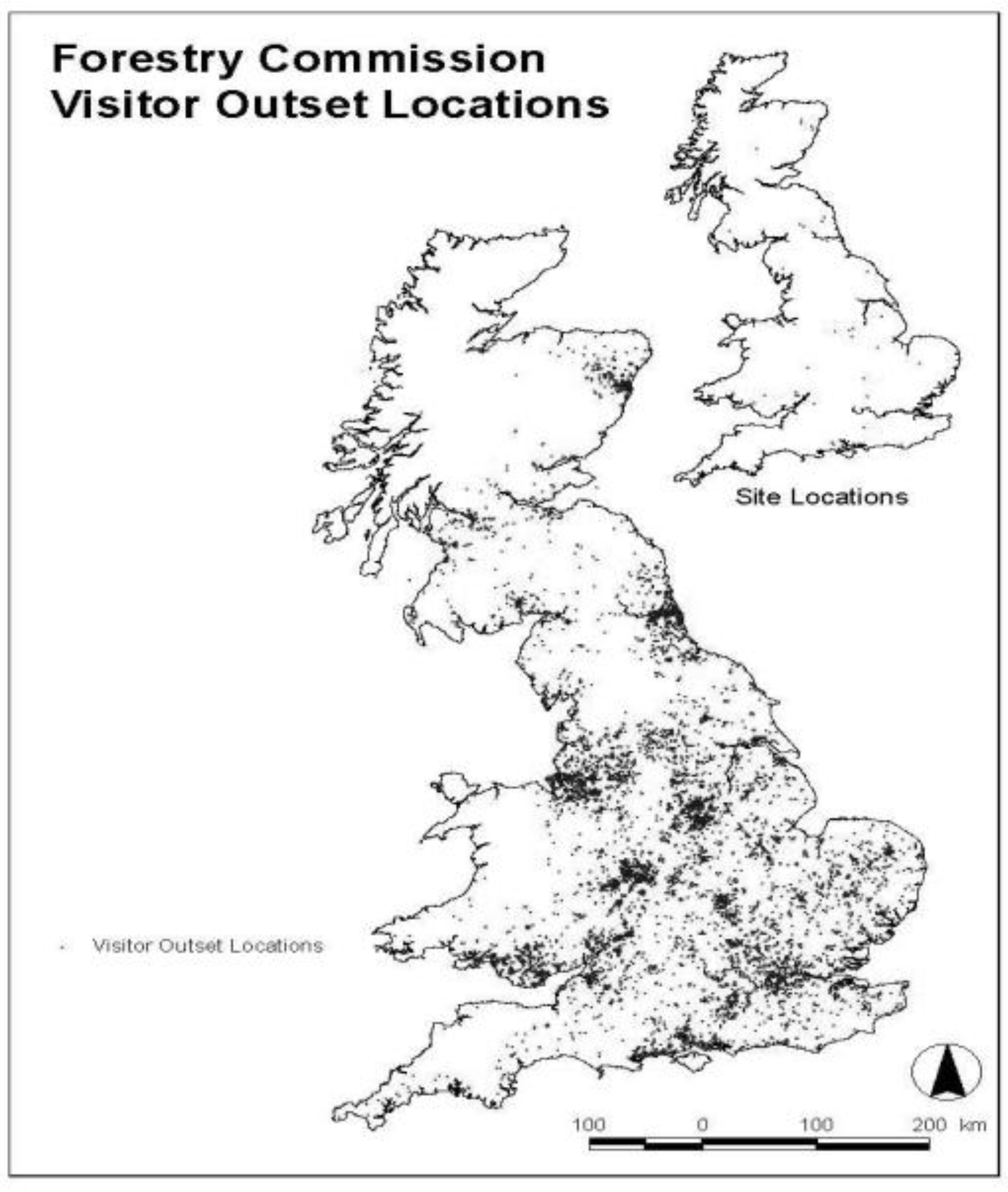
Accurate determination of the visitors’ home outset locations is a key piece of information as this provides the reference point for identification of the spatial drivers of visit demand. Postcodes of visitors’ home address locations were supplied and used to obtain an outset grid reference from the UK Central Postcode Directory (CPD). A total of 10,862 visitor interview records with usable postcodes were obtained, with corresponding residential locations being mapped in
Figure 1. So that geographical variations in visit rates could be examined, visitors were then assigned to outset zones based on their location. Outset zones were delineated based on the boundaries of Local Authority Districts, of which there were 451 in Great Britain at the time of analysis. Districts were chosen because they are large enough to each provide an adequate number of visitor arrivals from each, yet small enough to preserve an acceptable amount of homogeneity of population characteristics within their boundaries.
The calculation of travel times from the outset zone of residents to the site at which they were surveyed was undertaken using the ArcGIS package. The population weighted centroid of each outset zone was identified, and a route was developed to estimate the road based travel time from these centroids to all sites. Following the methodology of Brainard
et al. each section of the road network was accorded an average speed which reflected data from the Department of Transport which accounted for road designation, and urban/rural status [
14]. Travel times were then calculated between origins and destinations based on the assumption that visitors would choose the route which minimized time. Bateman
et al. show a very strong correspondence between such GIS generated travel times and those reported by woodland visitors interviewed in an on-site survey [
15].
Figure 1.
Visitor outset locations.
Figure 1.
Visitor outset locations.
As far as reasonable we sought to allow the analysis to identify potential substitute and complementary attractions by including data on a wide array of sites and facilities ranging from highly similar alternative forests and woodlands, through other outdoor open access sites (including heathland, sandy beaches, other coastline, rivers, inland waterways and canals, scenic areas, and national parks) and built amenities (zoos and wildlife parks, theme parks, National Trust properties, and historic houses). Towns and cities were identified so as to provide a surrogate indicator for some of the attractions not directly measured (e.g., cinemas, shopping centers, sports centers,
etc.). A variety of data sources were employed in this undertaking (including the remote-sensed CEH UK Land Cover Database for 1990, Bartholomew’s 1:250,000 Digital Database for Great Britain, the Scottish Council for National Parks, the (former) Countryside Commission for Scotland, internet sources (e.g.,
www.daysoutuk.com), the International Zoo Yearbook [
16] and the Good Zoo Guide [
17]).
Travel time values for substitutes were calculated using the same methodology as for the forest sites. However, the size of a substitute feature (e.g., an area of lakeland) may affect its accessibility as small sites can be treated as single point locations, but larger ones are likely to have a greater number of access points, with some closer and some further from outset locations. To account for this, accessibility scores were weighted according to the area covered by each substitute location so that scores were higher for smaller than larger features. Next, to place proportionally greater weight upon substitute features that were more proximal to visitor outset zone locations, these scores were further divided by the square of travel time from each outset origin. Previous research suggests that a squared power produced a good fit to observed visitor patterns [
18], so this was used.
In addition to the measure of weighted accessibility described above, a further indicator of substitute accessibility was computed as the percentage of each outset zone and surroundings covered by each substitute considered. To account for edge effects that may exist for residents living very close to district boundaries, the availability of substitute facilities in neighboring zones was considered by a procedure whereby each outset zone was amalgamated with its contiguous (boundary sharing) neighbors. The area of each substitute was then calculated for each of these amalgamated zones, and assigned to the principal outset zone. For linear features such as rivers and canals, a buffering technique was first applied to give the features a 20-metre width, which was assumed to be a reasonable approximation of real world widths.
As the propensity to seek generalized outdoor recreation experiences such as those provided by forestry may be associated with factors such as wealth, ethnicity, or household structure, a range of population socio-demographic characteristics for each outset zone were calculated from the UK Census of Population. In total 27 indicators were generated, covering transport availability, affluence and deprivation, education, ethnicity, age and family size. These indicators were also weighted by population density to compute the geographical distribution of population demographic characteristics that may influence visitor numbers.
2.2. Generation of Travel Cost Values
The transferable demand function is principally derived from regression models that predict visitation rates from outset zones. Typically, the dependent variable has a skewed distribution, reflecting that the majority of outset zones will provide no visitors to any given site, and hence a Poisson regression model [
19] suitable for count data analysis is employed, as was the case here.
For this study, the desired response variable yi would ideally be set as the total number of visitors to a site. However, observed visitor numbers will of course be conditioned by the degree of interview time on-site. To account for variations in survey effort, the number of interviews recorded at each site from each outset zone was divided by the amount of survey effort expended at that site. Survey effort was initially measured in hours, but this figure was divided by 24 so that the variable became a measure of effort in 24 hour periods. To further allow for variations in population across outset zones, the natural logarithm of the outset zone population was modeled as an offset. This means that our dependent variable is in effect a visitor rate.
One of the most fundamental problems of applying such models arises when the factors influencing the probability of visitors attending any individual site are seen to be operating at a variety of scales. For example, some sites may be either more or less attractive to visitors than others due to factors not captured in those site characteristics that are measured. This means such sites generate more or less visitors than would be predicted from the values of the predictor variables used to describe them. If this is the case the assumption of independence in the residuals from the regression model is violated. Due to such intra-unit correlation, the standard errors may be underestimated and the parameter estimates may be unreliable. Hence, to account for intra-unit correlation and produce efficient parameter estimates and standard errors, this study applied a multilevel (random coefficient) modeling approach using the MLWin software package [
20]. A two level structure was used of outset zones (level 1) nested within sites (level 2). Model building followed a staged approach which screened for multicollinearity within estimated models.
The model detailed above provides a prediction of the number of visitors interviewed at each site adjusted for survey effort. However, estimates of total visitation numbers within a specified period (here taken to be one year) are clearly of greater policy use. As we have discussed in other contexts, the conversion processes entailed in such translations can be a major source of error [
12]. This is typically a result of sparse aggregation data, in this case concerning the relationship between the numbers interviewed and actual annual arrivals. The only available data here were annual arrival estimates provided by the Forestry Commission for a subset of five sites included in the preceding analysis.
First, the predictions for each site were multiplied by a ratio of surveyed to unsurveyed (noted as being present but not interviewed) groups, based on information supplied by the Forestry Commission. Next, the temporal distribution of survey effort was directly incorporated in the regression model; variables were created detailing, for each site, the proportion of total effort undertaken in each month of the year. As there were too few surveys (and too little corresponding variation) within the months from October to April to justify their separate inclusion, only separate variables for each of the months May to September were included within these models. Thus their coefficients, measured as the proportion of total survey effect in each of the months, reflect departures from the base case of interviews outside this period. Estimated values for these coefficients conformed to expectations, with the greatest survey effort being expended in the summer period when visits are highest. Their control for seasonality effects upon survey effort meant that the inclusion of these variables within the model was justified on the grounds that it is likely to provide a superior basis for aggregation to annual visitor predications. The aggregation to annual visits was then achieved by multiplying the derived 24 hour predictions of arrivals (now adjusted for the seasonality in survey effort) by 365.25.
The models estimated here are amenable to calculations of travel cost values incurred by visitors for trips to woodlands, as the travel time variable can readily be related to travel cost estimates. In calculating travel cost, allowance was made for both travel expenditure and travel time values. The procedure used was as follows and is provided in Equation 1. The travel time
T (mins) of each party interviewed from outset location
j was multiplied by one-third [
21,
22] of the regional hourly wage rate
W (£) [
23] of outset location
j to calculate travel cost. Travel expenditure from outset location
j was calculated as the product of travel time from
j and an assumed average speed of 40 mph (specified as 0.67 miles per min) at average costs
C per mile. Summing the travel time value and travel expenditure resulted in the travel cost per group from
j, and this was multiplied by the total number of party visits
Pj from outset zone
j to calculate
j’s travel cost. To obtain the total value of travel costs per site
i, the travel costs per outset location were summed on a per site basis. Finally, resulting value was divided by the number of party visits
Si to the site to calculate the average value
Vi of a group visit to each site as shown in Equation (1)
Note that the value, Vi, does not include any element of the consumer surplus. The consumer surplus is the amount that forest visitors would have been willing to pay for their visits but were not required to do so. This value would be higher than our own estimate, which was based only on observed costs from travel. Thus our travel cost estimates may underestimate the true value of forest resources.
3. Results
3.1. The Best Fit Model for Day Visitors and Holidaymakers Combined
Table 2 shows the best fit model obtained to predict arrivals at survey sites. All prior expectations were satisfied. Controlling for population in each outset zone, by far the dominant factor determining visits is the negative influence of higher travel times. In many respects this is not surprising, however the strength and significance of this relationship has an important policy message, that it is the location of a site which primarily determines its level of use.
Table 2.
Best-fit model predicting recreational demand for a sample of Forestry Commission woodland sites across Britain. Dependent variable: rates of all visitor types (day-trip and holidaymaker) interviewed from each outset zone, adjusted for survey effort.
Table 2.
Best-fit model predicting recreational demand for a sample of Forestry Commission woodland sites across Britain. Dependent variable: rates of all visitor types (day-trip and holidaymaker) interviewed from each outset zone, adjusted for survey effort.
| Variable | Coefficient | s.e. | t | p |
|---|
| Constant | –11.730 | 1.775 | –6.608 | *** |
| Travel time to site | –2.563 | 0.026 | –98.615 | *** |
| Travel time to nearest inland water | 0.226 | 0.044 | 5.199 | *** |
| Travel time to nearest heathland | 0.170 | 0.023 | 7.274 | *** |
| Travel time to nearest coast | 0.153 | 0.022 | 6.888 | *** |
| Travel time to nearest National Trust Site | 0.105 | 0.040 | 2.642 | ** |
| Travel time to nearest large urban area | 0.044 | 0.014 | 3.095 | ** |
| Percentage of outset district and surrounding districts classified as woodland | –0.048 | 0.012 | –4.105 | *** |
| Percentage of outset district and surrounding districts classified as British Waterways canals | –0.018 | 0.002 | –9.588 | *** |
| Percentage of outset district households with children | 1.157 | 0.293 | 3.952 | *** |
| Percentage of outset district households with retired head | 0.668 | 0.234 | 2.854 | ** |
| Percentage of outset district population classified as Social Class 1 or 2 (affluent) | 0.703 | 0.086 | 8.173 | *** |
| Percentage of outset district population classified as non-white ethnicity | –0.109 | 0.029 | –3.710 | *** |
| Presence of visitor information centre at site | 0.640 | 0.273 | 2.341 | * |
| Early interviewing effort (7am to 10am) | –0.093 | 0.030 | –3.082 | ** |
| ‘Scottish Tour’ site indicator | 1.485 | 0.299 | 4.967 | *** |
| Between site variance parameter | 0.581 | 0.133 | 4.368 | *** |
One of the key contributions of our analysis is the intensive treatment of substitution effects upon visits. We assessed these effects through two sets of variables. A first set calculates substitute availability in terms of the proximity to potential arrival destinations. A second set of substitute indicators considered the intensity of recreational opportunities in and around outset zones.
Table 2 shows that the signs on the variables measuring the availability of both types of substitute are in the direction expected; those measuring travel time to substitutes are positive, illustrating that outset locations far from alternative substitutes will generate more woodland visits. The negative signs on those variables measuring the area of each substitute around the outset locations show that visitors will be less likely to visit woodlands if there are more alternative destinations around their home. Again this has a clear policy message that providing additional recreational facilities in an area which is already well endowed with such opportunities will generate lower levels of visitation than the provision of new sites in areas which are currently poorly provided for. While commonsense, to our knowledge this is the first time such relationships have been quantified.
Table 2 continues by providing evidence of the extent to which the socio-economic and demographic characteristics of outset zones influence the rate of visitation from those zones. Areas which have higher levels of young children, retired or higher social classes are all associated with elevated numbers of visitors. This result suggests that families with young children may well be more disposed to outdoor activities and that the retired have less time constraints than others. Similarly higher income groups enjoying greater mobility are more likely to engage in woodland recreation. This latter relation is likely to substantially reflect the present spatial distribution of woodlands which are generally not located within low income areas. A policy of locating woodlands nearer to low income households should go some way to allowing for this effect. In Great Britain the increasing importance of agri-environmental schemes as a source of income for farmers means that the conversion of land from arable to woodland use is a more feasible proposition than has been the case in the past, and Government funding has also been made available for the creation of ‘Community Woodlands’, although the benefits of such initiatives take many years to be fully realized. Hence in the shorter term other possibilities, such as enhancing recreational opportunities in existing woodlands for low income groups, may also be important [
24]. Even controlling for socio-economics, the model shows that areas with more ethnic populations yield fewer visitors, a result that may reflect tastes or imperfect control for the lower accessibility of woodlands to the primarily urban ethnic community.
Out of the numerous site facility and quality variables gathered, only the presence of information boards at a site proved to exert a significant impact upon the numbers interviewed. Even this may well be acting as a proxy for other facilities or site characteristics or a problem of endogeneity as the decision to install a notice board may well depend on there being sufficient visitors to warrant its construction. What this does show is that, in comparison to the strength of the travel time variable for example, it is the location of recreational woodland rather than its specific facilities (above the common facilities of woodland walks and car parking) which determines visitation.
Two final control variables were significant. Least interesting of these is the negative coefficient of the ‘Early interviewing effort (7 am to 10 am)’ variable which allows for variation in the distribution of survey effort across the day, here reflecting the lower interview rate achieved when interviewers had higher proportions of their survey effort focused upon very early hours of the day when visitor numbers were low. More interesting is the fact that sites located in Scotland (labeled as ‘Scottish tour’ sites in
Table 2) have a higher number of visitors interviewed than might be expected from their characteristics. Discussions with Forestry Commission staff suggests that this may reflect the influence of touring holidaymakers increasing the number of visitors above that which would otherwise be expected for sites with such small local populations.
Examination of the between-site (level 2) residual variance showed no particular trend across sites. We believe the best-fit model is richer than models provided by most previous research and consistently in accordance with prior expectations derived from theory and previously observed empirical regularities. Given this, it appears that the model should be suitable for predicting visitor trends across all sites, which we now consider.
3.2. Transferring the Best-Fit Model
The main question after estimating a transferable visitation rate function is if the model can provide useful input to the real world planning and decision-making process.
Table 3 details predicted arrivals for each site, based on the coefficients obtained in the best-fit regression model when that site was omitted (
i.e., adhering to best-practice, out-of-sample prediction methods). Sites marked with an asterisk in the table are those located in Scotland. This provides an assessment of the likely performance of the model in a policy situation where no survey based information is known about a given target site. Inspection of
Table 3 shows that while the overall trend of results is encouraging, there is substantial error at certain sites with both under- and over predicted numbers.
Table 3.
Transferred predictions of interview numbers for all visitor types from the best-fit model.
Table 3.
Transferred predictions of interview numbers for all visitor types from the best-fit model.
| Site Number | Site Name | Observed Visitor Numbers Surveyed | Predicted Visitor Numbers Surveyed | Difference Observed-Predicted | Ratio Observed-Predicted |
|---|
| 3 | Afan Argoed | 458 | 1086.61 | –628.61 | 2.37 |
| 6 | Alice Holt | 217 | 701.55 | –484.55 | 3.23 |
| 8 | Back O Bennachie* | 100 | 71.95 | 28.05 | 0.72 |
| 9 | Beechenhurst | 128 | 111.33 | 16.67 | 0.87 |
| 14 | Black Rocks | 161 | 303.21 | –142.21 | 1.88 |
| 15 | Blackwater | 179 | 305.06 | –126.06 | 1.70 |
| 17 | Blidworth Woods | 216 | 906.70 | –690.70 | 4.20 |
| 18 | Bolderwood | 343 | 668.10 | –325.10 | 1.95 |
| 20 | Bourne Wood | 211 | 132.35 | 78.65 | 0.63 |
| 33 | Chopwell | 125 | 94.50 | 30.50 | 0.76 |
| 34 | Christchurch | 132 | 50.38 | 81.62 | 0.38 |
| 40 | Countesswells* | 212 | 121.69 | 90.31 | 0.57 |
| 43 | Dean Cycle Centre | 222 | 180.60 | 41.40 | 0.81 |
| 44 | Dalby | 305 | 225.60 | 79.40 | 0.74 |
| 46 | Delamere | 684 | 1086.18 | –402.18 | 1.59 |
| 49 | Dibden | 215 | 57.71 | 157.29 | 0.27 |
| 51 | Donview* | 144 | 128.88 | 15.12 | 0.90 |
| 61 | Garwnant | 358 | 286.10 | 71.90 | 0.80 |
| 66 | Glentrool* | 321 | 167.45 | 153.55 | 0.52 |
| 68 | Grizedale | 265 | 107.09 | 157.91 | 0.40 |
| 72 | Hamsterley | 160 | 134.23 | 25.77 | 0.84 |
80
83 | Kielder
Kings Wood | 104
102 | 28.08
134.84 | 75.92
–32.84 | 0.27
1.32 |
| 84 | Kirkhill* | 207 | 935.21 | –728.21 | 4.52 |
| 86 | Kylerhea* | 210 | 59.65 | 150.35 | 0.28 |
| 95 | Mabie* | 686 | 618.66 | 67.34 | 0.90 |
| 111 | Queens View* | 270 | 307.90 | –37.90 | 1.14 |
| 117 | Salcey | 196 | 550.64 | –354.64 | 2.81 |
| 119 | Sherwood Pines | 680 | 2317.93 | –1637.93 | 3.41 |
| 121 | Simonside Hills | 136 | 25.42 | 110.58 | 0.19 |
| 126 | Symonds Yat | 255 | 112.73 | 142.27 | 0.44 |
| 128 | Thetford High Lodge | 687 | 650.38 | 36.62 | 0.95 |
| 129 | Thieves Wood | 307 | 801.27 | –494.27 | 2.61 |
| 130 | Thrunton Woods | 142 | 49.94 | 92.06 | 0.35 |
| 134 | Tyrebagger* | 149 | 612.53 | –463.53 | 4.11 |
| 137 | Waters Copse | 172 | 97.09 | 74.91 | 0.56 |
| 141 | Wendover | 117 | 211.98 | –94.98 | 1.81 |
| 143 | Westonbirt Ab | 440 | 174.80 | 265.20 | 0.40 |
| 147 | Willingham Woods | 176 | 158.90 | 17.10 | 0.90 |
| 153 | Wyre | 670 | 1749.85 | –1079.85 | 2.61 |
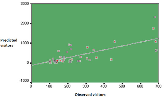
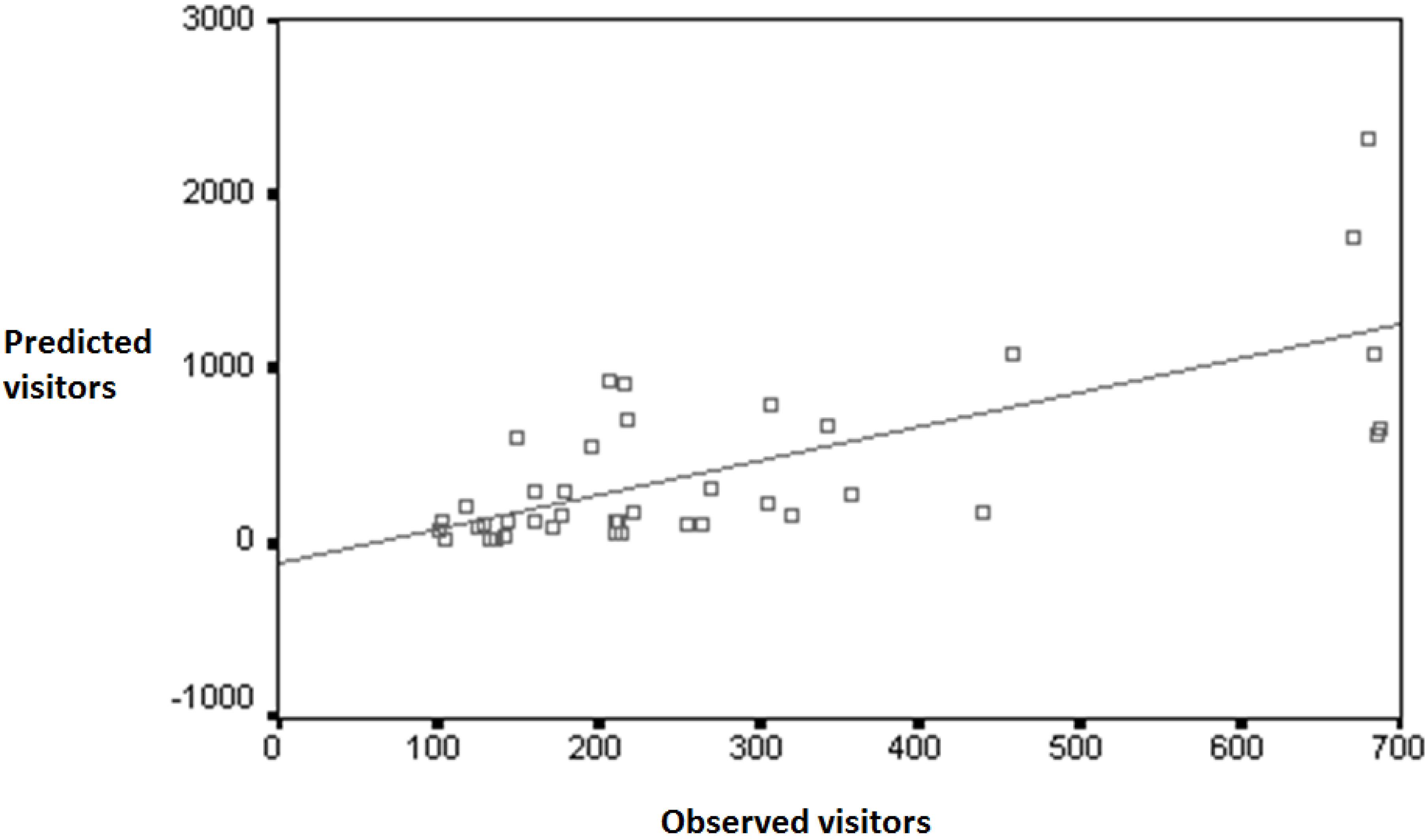
In order to further inspect the relationship between observed and predicted interview numbers,
Figure 2 provides a measure of observed
versus predicted visits (using our model from
Table 2). The included regression line indicates the expected positive relation between observed and predicted values. According to a simple correlation test (ρ = 0.709; p < 0.001) and a χ2-test examining the ability of the model to predict visits (χ2 = 11.00; p < 0.001), the model performs well overall. However, inspection of
Figure 2 suggests some degree of systematic deviation between predicted and observed visit (interview) rates. In particular observed visit rates appeared to be truncated at roughly 700 interviews. It may be that interviewers were instructed to finish interviewing, or decided to do so of their own accord, once this level was reached. Accepting that this will militate against a clean test of our model it is nevertheless clear that this best-fit model differentiates well between sites with high and low visitor interview numbers.
Figure 2.
Plot of observed and predicted visitor interview numbers.
Figure 2.
Plot of observed and predicted visitor interview numbers.
3.3. Estimates of Annual Arrivals
The output from the regression model was then used to predict annual arrivals at the subset of sites at which actual arrival data was available as a comparator. Unfortunately the Forestry Commission was only able to supply estimates of total visitor numbers for five of the sites in their survey dataset. Even these were supplied with strong caveats regarding their likely accuracy; hence we have no perfect criterion measure of actual visits and have to accept these rather imperfect estimates at this restricted number of locations. Given these caveats, comparisons at these sites are given in
Table 4.
Table 4.
Comparison of Forestry Commission and model estimates of annual visits to five woodlands.
Table 4.
Comparison of Forestry Commission and model estimates of annual visits to five woodlands.
| Site Name | Forestry Commission Estimate of the Number of Party Visits p.a. | Model Prediction of Number of Party Visits p.a. |
|---|
| Beechenhurst | 72,845 | 79,504 |
| Blidworth Woods | 63,849 | 116,553 |
| Chopwell | 33,708 | 71,334 |
| Mabie | 51,704 | 56,561 |
| Symonds Yat | 77,525 | 108,154 |
| Total | 299,631 | 432,106 |
The overall correspondence between Forestry Commission and model-derived estimates of arrivals has a ratio of 1.44. Given the prior caveats, the comparative ranking of sites is perhaps more important. The top three sites and lower two sites are consistent across the two sets of estimates suggesting that the model can robustly distinguish between high and low visitation sites. Given the uncertainty with regard to the Forestry Commission estimates of overall annual totals, we feel this is a satisfactory finding.
3.4. Estimation of Travel Cost Values
Using our previously described methodology, travel cost values were generated separately for all visitors, day-trippers and holidaymakers to yield the values detailed in
Table 5. As expected, travel costs are higher for holidaymaker than day-trip visitors. It is important to recall that the values detailed in
Table 5 are travel costs rather than consumer surplus values which would require further information than was available in the Forestry Commission data (see [
2] for details). Combined with the predicted annual visitor numbers from the 5 sites for which Forestry Commission estimates were available, the travel cost values placed by visitors on each site can be estimated and are presented in
Table 6. A comparison of the values in
Table 6 with the regression model coefficients used to generate them (
Table 2), shows the predominant driver of differences in site value is population accessibility (specified from travel time), with the accessibility of substitute sites being of secondary importance, and site characteristics having the smallest influence.
Table 5.
Travel cost value for all visitors, day-tripper and holidaymakers for each site.
Table 5.
Travel cost value for all visitors, day-tripper and holidaymakers for each site.
| Site Number | Site Name | All Visitors | Day Visitors | Holiday Visitors |
|---|
| 3 | Afan Argoed | 8.62 | 4.02 | 31.76 |
| 6 | Alice Holt | 4.30 | 4.09 | 11.10 |
| 8 | Back O Bennachie | 12.24 | 6.61 | 77.01 |
| 9 | Beechenhurst | 14.00 | 8.79 | 24.26 |
| 14 | Black Rocks | 9.32 | 5.17 | 22.78 |
| 15 | Blackwater | 19.62 | 8.16 | 29.85 |
| 17 | Blidworth Woods | 2.95 | 2.74 | 26.46 |
| 18 | Bolderwood | 18.71 | 6.58 | 27.97 |
| 20 | Bourne Wood | 5.73 | 4.88 | 21.10 |
| 33 | Chopwell | 4.02 | 4.00 | 5.25 |
| 34 | Christchurch | 18.15 | 14.72 | 18.79 |
| 40 | Countesswells | 3.63 | 2.79 | 62.24 |
| 43 | Cycle Centre | 13.13 | 7.93 | 25.21 |
| 44 | Dalby | 20.54 | 12.06 | 29.54 |
| 46 | Delamere | 4.53 | 4.44 | 6.62 |
| 49 | Dibden | 3.85 | 3.48 | 12.25 |
| 51 | Donview | 15.48 | 8.13 | 66.92 |
| 61 | Garwnant | 11.12 | 5.22 | 30.72 |
| 66 | Glentrool | 35.77 | 13.84 | 47.78 |
| 68 | Grizedale | 25.59 | 10.38 | 30.83 |
| 72 | Hamsterley | 16.49 | 11.14 | 32.65 |
| 80 | Kielder | 35.79 | 19.50 | 45.00 |
| 83 | Kings Wood | 17.38 | 15.62 | 41.27 |
| 84 | Kirkhill | 5.11 | 3.26 | 41.53 |
| 86 | Kylerhea | 85.83 | 58.30 | 87.13 |
| 95 | Mabie | 20.28 | 6.43 | 36.47 |
| 111 | Queens View | 57.25 | 27.19 | 62.84 |
| 117 | Salcey | 3.78 | 3.14 | 17.22 |
| 119 | Sherwood Pines | 8.95 | 3.85 | 25.13 |
| 121 | Simonside Hills | 17.66 | 8.74 | 41.57 |
| 126 | Symonds Yat | 19.76 | 11.76 | 25.19 |
| 128 | Thetford High Lodge | 11.64 | 7.74 | 25.74 |
| 129 | Thieves Wood | 2.58 | 2.52 | 12.78 |
| 130 | Thrunton Woods | 19.34 | 6.01 | 42.45 |
| 134 | Tyrebagger | 4.56 | 3.39 | 22.93 |
| 137 | Waters Copse | 18.98 | 8.24 | 27.28 |
| 141 | Wendover | 4.96 | 4.61 | 12.78 |
| 143 | Westonbirt Ab | 11.75 | 8.59 | 24.91 |
| 147 | Willingham Woods | 8.28 | 7.18 | 22.92 |
| 153 | Wyre | 6.81 | 4.65 | 18.95 |
Table 6.
Estimated travel cost values to five woodlands for converted model predictions of annual visitor numbers.
Table 6.
Estimated travel cost values to five woodlands for converted model predictions of annual visitor numbers.
| Site Name | Travel Cost Value |
|---|
| Beechenhurst | £990,619 |
| Blidworth Woods | £564,116 |
| Chopwell | £374,503 |
| Mabie | £1,417,418 |
| Symonds Yat | £1,211,324 |
| Total | £4,557,980 |
4. Discussion and Conclusions
The main objective of the study was to develop a model to predict visitation rates at recreational sites, taking account of the accessibility and facilities of the resource, the availability of substitutes and variation in population characteristics. A GIS-based methodology was developed to analyze the spatial distribution of these various determinants which were then modeled within a hierarchical (multilevel) zonal travel cost framework. Allowance was made for survey effort and the resulting model performs well against all prior expectations. The strongest predictor of visitor arrivals is accessibility (travel time) but strongly significant substitution effects were identified for competing natural and man-made resources. Household characteristics also affect visitation rates in expected ways.
The methodology developed through this paper allows the policy analyst to parameterize a wide set of visit demand determinants. As such we refine a highly flexible policy formulation and analysis tool which sits well with the drive of governments internationally towards evidence-based policy making.
The research is presented with some caveats. The travel cost methodology adopted assumes that the woodland at which each survey was undertaken was the sole destination on the trip, and also that no pleasure, or utility, was obtained from the journey. In situations where this was not the case, for example where enjoyment was derived from scenic driving or sight-seeing along the way, the value attached to the recreational site may be overestimated. In this respect, WTP values from the analysis may overestimate true figures. We also benefitted here from Great Britain being an island state, meaning we did not have the problem of ‘edge effects’ (e.g., the proximal availability of substitutes that we did not have information on across a border) that would occur if our analysis had been based on a jurisdiction surrounded by others. Although information was available that allowed day visitors and holidaymakers to be differentiated, no details were recorded on the holiday location of holidaymakers, and hence our analysis was based upon the measurement of travel times from home for this group. This restricted the ability of our analysis to differentiate between the motivations for visiting a particular region for a holiday, and the choice the specific forest site. There was also evidence of truncation of interview numbers at heavily visited locations, suggesting that there were survey capacity limitations that may have prevented us differentiating some sites with very high visitor numbers. A further restriction lies in the fact that the Forestry Commission were unable to supply large numbers of annual visitor numbers for calibration purposes and even those that were provided came with strong caveats regarding their likely accuracy. This is not an unusual state of affairs. While the UK has good survey data concerning the outdoor activities of households, this is not spatially explicit and there is a clear need for such data to inform both research and planning.
The methodology developed here is deliberately designed for general applicability and transfer. A notable feature is the utilization of generally available national coverage databases for generating the predictors of visits. Key data sources were the Ordnance Survey and UK Census; data that are available to researchers and policy makers alike. Furthermore, while the initial processing of data takes some time, once generated the data surfaces should be valid for some considerable time and require only occasional updating. Road networks, the availability of substitutes and the socioeconomic and demographic profiles of regions only change gradually with time and we estimate than updating would only be needed at most every five years with longer periods (such as the ten year gap between Census dates) probably being acceptable for most analyses. Of course, one disadvantage of this focus on infrastructure and physical features is that matters of culture and perception are not encompassed. For example, authors such as Stedman [
25] have shown that physical features do contribute to feelings of sense of place in forest environments, yet cultural components such as constructed meanings and place attachment can also important. These undoubtedly also contribute to the value of forest resources, yet we were not able to incorporate such considerations in our work. One implication of this is that our models may be more appropriate for strategic-level planning where population-wide decisions are being made. However, our failure to incorporate the more experiential characteristics of sites into our transfer functions might mean that further surveys would be required for operational considerations, such as those associated with woodland design.
Individual analyses can of course readily posit policy induced changes such as the creation of new recreational opportunities, although it should be noted that different resource types may have differing transition profiles; the creation of a new lake may result in a rapid transition to maximum visitation levels but this may be less true for woodlands where the impact upon visitation of the naturally slow rate of forest establishment needs to be allowed for.
Whilst a number of limitations of the work have been highlighted, the function transfer model developed here explicitly addresses one of the major empirical problems facing successful function transfer; spatial complexity between sites. Previous work has faced severe problems in addressing this issue. The issue is important because even the most fundamental predictor of visit numbers, travel time, has strong spatial heterogeneity. Geographical Information Systems coupled with high quality digital map databases provide novel opportunities to produce measures of the underlying determinants of recreational visits. Furthermore, these measures can be obtained in a consistent manner for both surveyed study sites and un-surveyed target sites. It is this consistency, compatibility, availability and richness of measures which provides the quantitative measurements vital for successful function transfer. Although we find that the location characteristics are still the main drivers of site visits, we argue that for increased reliability future recreation and valuation studies, using both revealed and stated preference methods, should attempt to include indicators that reflect the availability of different type of substitutes in their value functions.
It is likely that the demand from decision makers for benefit transfer applications will continue to increase in the future, primarily due to the increasing emphasis being placed on outdoor recreation and the expense and time-consuming nature of survey data collection. Inexpensive benefit transfer estimates are frequently required as organizations now have to be more commercially accountable. Consequently improving the robustness of benefit transfer techniques is likely to remain a topic for significant research in the future.

