Integrated AI Framework for Sustainable Environmental Management: Multivariate Air Pollution Interpretation and Prediction Using Ensemble and Deep Learning Models

Abstract

Accurate prediction, forecasting and interpretability of air pollutant concentrations are important for sustainable environmental management and protecting public health. An integrated artificial intelligence (AI) framework is proposed to predict, forecast and analyse six major air pollutants, such as particulate matter concentrations (PM_2.5 and PM₁₀), ground-level ozone (O₃), carbon monoxide (CO), nitrogen dioxide (NO₂), and sulphur dioxide (SO₂), using a combination of ensemble and deep learning models. Five years of hourly air quality and meteorological data are analysed through correlation and Granger causality tests to uncover pollutant interdependencies and driving factors. The results of the Pearson correlation analysis reveal strong positive associations among primary pollutants (PM_2.5–PM₁₀, CO–nitrogen oxides NO_x and VOCs) and inverse correlations between O₃ and NO_x (NO and NO₂), confirming typical photochemical behaviour. Granger causality analysis further identified NO₂ and NO as key causal drivers influencing other pollutants, particularly O₃ formation. Among the 23 tested AI models for prediction, XGBoost, Random Forest, and Convolutional Neural Networks (CNNs) achieve the best performance for different pollutants. NO₂ prediction using CNNs displays the highest accuracy in testing (R² = 0.999, RMSE = 0.66 µg/m³), followed by PM_2.5 and PM₁₀ with XGBoost (R² = 0.90 and 0.79 during testing, respectively). The Air Quality Index (AQI) analysis shows that SO₂ and PM₁₀ are the dominant contributors to poor air quality episodes, while ozone peaks occur during warm, high-radiation periods. The interpretability analysis based on Shapley Additive exPlanations (SHAP) highlights the key influence of relative humidity, temperature, solar brightness, and NO_x species on pollutant concentrations, confirming their meteorological and chemical relevance. Finally, a deep-NARMAX model was applied to forecast the next horizons for the six air pollutants studied. Six formulas were elaborated using input data at times (t, t − 1, t − 2, …, t − n) to forecast a horizon of (t + 1) hours for single-step forecasting. For multi-step forecasting, the forecast is extended iteratively to (t + 2) hours and beyond. A recursive strategy is adopted for this purpose, whereby the forecast at (t + 1) is fed back as an input to generate the forecasts at (t + 2), and so forth. Overall, this integrated framework combines predictive accuracy with physical interpretability, offering a powerful data-driven tool for air quality assessment and policy support. This approach can be extended to real-time applications for sustainable environmental monitoring and decision-making systems.

1. Introduction

Inadequate air quality has well-documented adverse impacts on human health and the environment [1]. Major pollutants such as PM_2.5, PM₁₀, O₃, CO, NO₂, and SO₂ in urban areas pose significant risks, so accurate prediction and precise short-term forecasting of their concentrations can support early warning and mitigation.

Recent advances in air-quality modelling, prediction and forecasting combine rich observational datasets with powerful machine learning (ML) and deep learning (DL) methods to improve prediction and forecasting accuracy and interpretability. Most of them highlight a trend towards hybrid, multivariate, and ensemble models that improve prediction accuracy and interpretability.

Table 1. Recent advanced approaches for predicting various air atmospheric pollutants.

Model/Approach Name	Key Features	Primary Application/Target	Key Findings/Performance	Reference
MVAR (MultiVariate AutoRegressive)	Multivariate Autoregressive Training; Meteorological Coupled Spatial Transformer; handles 120 h forecasts.	Multiple pollutants (PM2.5, PM10, O3, CO, NO2, SO2) simultaneously.	Reduces dependency on long-time-window data; learns interactions between pollutants and their spatial responses.	[2]
AirCast	Fuses weather & chemical data; Vision Transformer; frequency-weighted MAE loss function.	PM2.5 and PM10, especially during rare extreme events (e.g., dust storms).	33% reduction in PM2.5 forecast error vs. persistence baseline; outperformed CAMS physics model in regional forecasts.	[3]
Stacking Ensemble Model	Combines predictions from multiple base models (e.g., MLP, SVR, RF) in a stacking framework.	PM2.5 concentration forecasting.	Superior results: MAE (6.67), RMSE (8.80), and R2 (0.91) outperformed traditional single models.	[4]
AQP-EDLMRA	Ensemble voting of LSTM, DBN, SAE; hyperparameters optimised with Mud Ring Algorithm.	Prediction of multiple air pollutants (PM2.5, NOx, COx, SOx).	Demonstrated improved forecasting performance in comparative tests on air quality data.	[5]
MVAR (MultiVariate AutoRegressive)	Multivariate Autoregressive Training; Meteorological Coupled Spatial Transformer; handles 120 h forecasts.	Multiple pollutants (PM2.5, PM10, O3, CO, NO2, SO2) simultaneously.	Reduces dependency on long-time-window data; learns interactions between pollutants and their spatial responses.	[2]
Autoencoders (AEs) & Sparse AEs (SAEs)	Uses AEs/SAEs for feature compression and denoising; models pollution as a classification task (quartiles).	Next-hour concentration of NO2, PM10, and SO2 in a port-industrial area.	AEs are better for moderate levels; SAEs are better for extreme concentrations (Q1 & Q4); the combination enhances forecasting.	[6]
LSTM (Long Short-Term Memory)	Captures long-term temporal dependencies; sequence-to-sequence architecture; hyperparameter tuning (layers, hidden units, dropout).	Time-series forecasting of O3 and other pollutants using meteorological and pollutant data.	Outperformed standard ANN for daily O3 prediction (R2 ≈ 0.69 vs. 0.68). Effective for short-term and recursive multi-step forecasting.	[7]
CNN (Convolutional Neural Network)	Extracts spatial structures and local patterns; it can process gridded data from spatially interpolated sensors.	Short-term PM2.5/PM10 forecasting using spatially distributed station data.	“Interpolated CNN” achieved R2 > 0.97 for short-term PM prediction in Korea, showing strong spatial pattern extraction.	[8]
CNN–LSTM Hybrid (with Attention)	Combines spatial feature extraction (CNN) and temporal sequence modelling (LSTM); attention mechanism enhances feature weighting.	O3 and PM prediction integrating spatial-temporal dependencies.	CNN + LSTM + Attention model achieved R2 = 0.97 for ozone forecasting, demonstrating superior spatio-temporal modelling capacity.	[9]
Transformer Network	Employs self-attention for global temporal dependency modelling; supports direct multi-step prediction; effective for long-term dependencies.	Long-term air quality forecasting (PM, O3, etc.) using pollution and meteorological data.	Shown to outperform traditional models for 7–24 h forecasts; well-suited for long-horizon predictions due to attention mechanism.	[10]
Hybrid Spatio-Temporal (e.g., KSC-ConvLSTM, GAT-BiLSTM)	Integrates KNN for nearest-neighbour data selection, attention-based ConvLSTM, and/or graph layers to capture spatial correlations.	Spatio-temporal PM2.5 prediction using geographically distributed data.	KSC-ConvLSTM outperformed CNN-LSTM for Beijing PM2.5 forecasting; GAT-BiLSTM effectively captures spatial relations.	[11,12]
Ensemble and Feature-Level Hybrids	Combines multiple model predictions (e.g., LSTM, CNN-LSTM, Transformer) via averaging or meta-learning; integrates pollution-weather feature embeddings.	Robust and adaptive air quality forecasting across varying meteorological regimes.	Ensembling improved reliability and generalisation; feature-level fusion enhanced detection of local/global and linear/nonlinear relationships.	[11]

summarises key advanced approaches:

However, in most cases, high-quality pre-processing is very important for these models. All data should be standardised and normalised, missing entries should be removed or imputed (e.g., using linear interpolation or time-series imputation), and outliers and anomalies should be identified and removed. Multicollinearity can be decreased using correlation analysis and methods such as PCA [12]. Temperature, wind, and humidity, for example, are critical in influencing the dispersion of air pollutants, and their inclusion significantly enhances the accuracy of AI-based models, according to previous research, which emphasises the need for careful integration of meteorological factors [11]. For instance, ozone (O₃) production is strongly influenced by high temperatures and sunlight [13], whereas PM may be washed away by precipitation [14]. Wind speed and direction, as well as rainfall, may also directly affect the precursors of air pollutants. The most pertinent predictors can be found using feature-selection algorithms, such as El Mghouchi’s GEO-based FS [14]. Building on the framework outlined in [14], this study aims to deepen understanding of the complex interactions among major air pollutants and various atmospheric and meteorological variables.

The specific objectives are as follows:

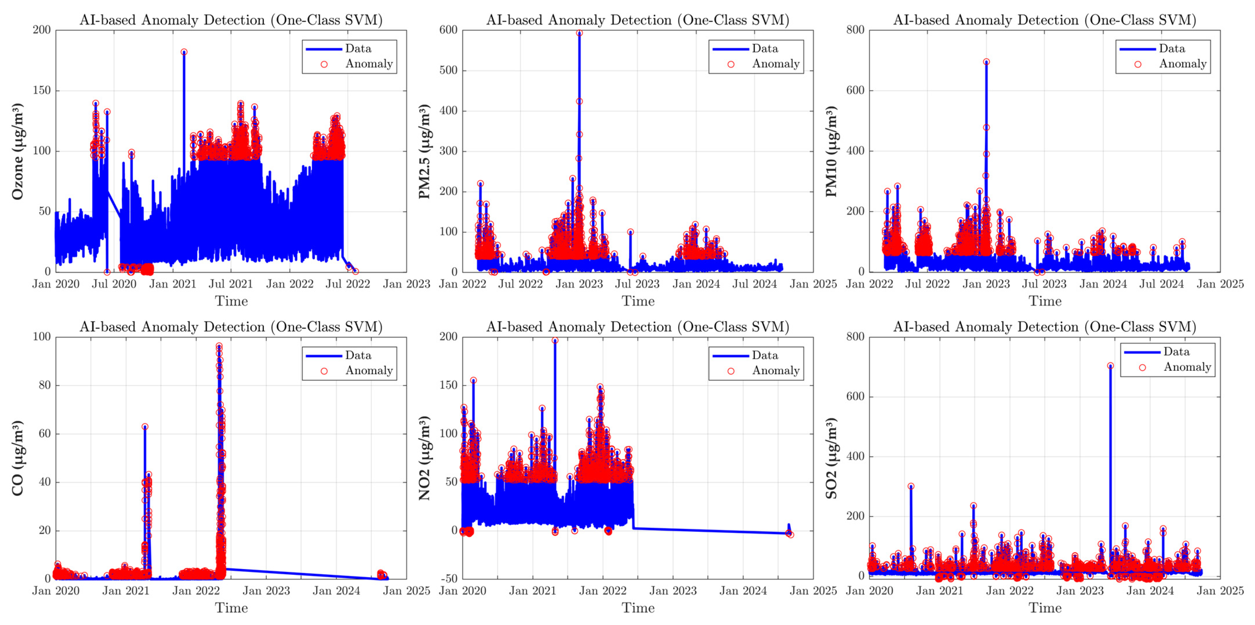
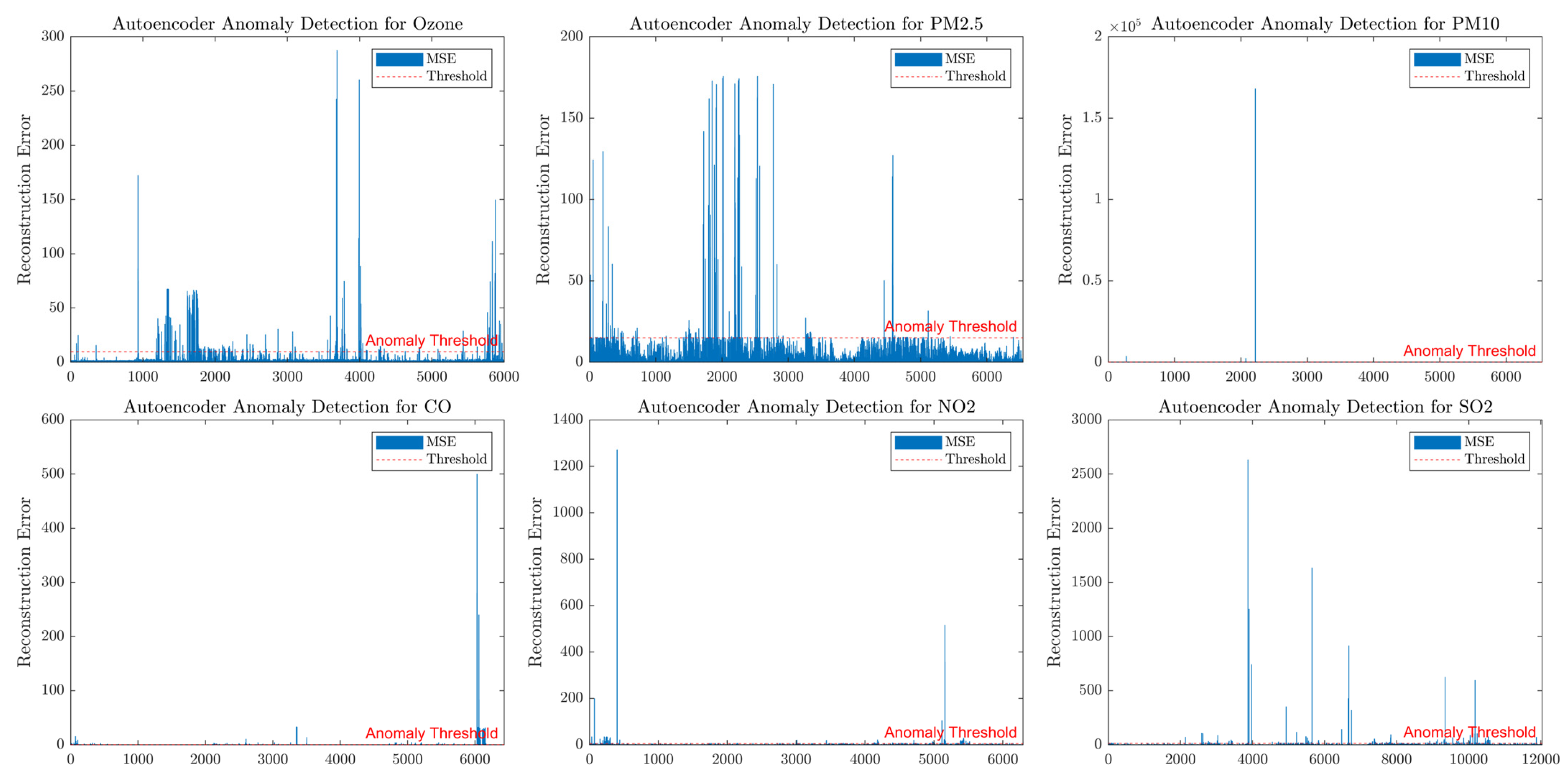
• Data Pre-processing: Implement robust pre-processing procedures, including advanced imputation methods for short missingness intervals (MICE and KNN), anomaly detection (OCSVM and autoencoders), and frequency-domain denoising (Singular Spectrum Analysis), to ensure high data quality and reliability. The result for this analysis is provided in Appendix A (Figure A1, Figure A2, Figure A3 and Figure A4).
• Trend and Temporal Variability Analysis: Investigate the temporal patterns and long-term trends of six key air pollutants—PM_2.5, PM_10, O₃, CO, NO₂, and SO₂ and the Air Quality Index (AQI). Each pollutant exhibits distinct temporal behaviours influenced by emission sources, atmospheric chemistry, and meteorological dynamics.
• Correlation and Relationship Assessment: Examine the interrelations between the six pollutants and meteorological variables through regression and cross-correlation analyses to quantify their mutual dependencies and influence mechanisms.
• Causality Analysis: Apply the Granger causality test to identify potential directional relationships between meteorological parameters and pollutant concentrations, determining whether past values of one variable can reliably predict future values of another.
• AI-based prediction models: Our approach involved implementing 23 ML and DL algorithms, optimising parameters via Randomised Search CV, Grid Search and Adam Optimizer (

  Table A1. Hyperparameter Search Space for Machine Learning Models.

  Model	Optimisation Method	Hyperparameter Name	Search Range/Grid
  Random Forest (RF)	RandomizedSearchCV	n_estimators	[100, 300, 500]
  		max_depth	[10, 20, 30, None]
  		min_samples_split	[2, 5, 10]
  Gradient Boosting (GBoost)	RandomizedSearchCV	n_estimators	[100, 300, 500]
  		learning_rate	[0.01, 0.05, 0.1]
  		max_depth	[3, 5, 7]
  XGBoost	RandomizedSearchCV	n_estimators	[100, 500, 1000]
  		learning_rate	[0.01, 0.05, 0.1, 0.3]
  		max_depth	[3, 5, 7, 9]
  		colsample_bytree	[0.6, 0.8, 1.0]
  Support Vector Machine (SVM)	RandomizedSearchCV	C	[0.1, 1, 10, 100]
  		kernel	[‘rbf’, ‘linear’, ‘poly’]
  K-Nearest Neighbours (KNN)	RandomizedSearchCV	n_neighbors	[3, 5, 7, 11, 15]
  		weights	[‘uniform’, ‘distance’]
  Decision Tree (DT)	RandomizedSearchCV	max_depth	[None, 10, 20, 50]
  		min_samples_leaf	[1, 2, 4]
  Tree Bagger (TreeBag)	RandomizedSearchCV	n_estimators	[10, 50, 100]
  		max_samples	[0.5, 0.7, 1.0]
  Gaussian Process (GPR)	RandomizedSearchCV	alpha	[1 × 10−10, 1 × 10−5, 1 × 10−2]
  		kernel	[RBF, Matern, RationalQuadratic]
  Kernel Ridge (KRR)	RandomizedSearchCV	alpha	[0.1, 1.0, 10.0]
  		gamma	[0.01, 0.1, 1, 10]
  Linear Ridge (LRR)	RandomizedSearchCV	alpha	[0.01, 0.1, 1.0, 10.0, 100.0]
  Bayesian Ridge (BayesLR)	RandomizedSearchCV	n_iter	[300]
  		alpha_1/lambda_1	[1 × 10−6, 1 × 10−4]

  and

  Table A2. Configuration and Optimisation of Deep Learning & Specialised Models.

  Model Class	Specific Model(s)	Hyperparameter/Configuration	Value/Search Space	Optimisation Strategy
  FNN/ANN/DNN	ANN, FNN, DNN, FCNN	Hidden Layers	[1, 2, 3]	Adam Optimizer + Early Stopping
  		Neurons per Layer	[32, 64, 128, 256]
  		Activation	ReLU (Hidden), Linear (Output)
  		Dropout Rate	[0.0, 0.2, 0.5]
  CNN	Convolutional Neural Network	Conv1D Layers	[1, 2]	Adam Optimizer + Early Stopping
  		Filters	[16, 32, 64]
  		Kernel Size	[3, 5, 7]
  		Dense Neurons	[50, 100]
  RNN	LSTM, LSTM-RNN	LSTM Layers	[1, 2]	Adam Optimizer + Early Stopping
  		Units	[32, 64, 128]
  ResNet	Residual Neural Network	Residual Blocks	[2, 3]	Adam Optimizer + Early Stopping
  		Filters	[32, 64]
  ELM	Extreme Learning Machine	Hidden Neurons	[500, 1000, 1500]	Random Projection (Fixed Weights)
  GAM	Generalised Additive Model	n_splines	[20, 25, 30]	Grid Search via GCV

  in the Appendix A). We combined the best-performing model with feature selection strategies to create a high-precision hybrid AI model for air pollutant prediction.
• Feature Selection (FS): We employed statistical and machine learning-based feature selection methods to identify the most informative predictors, improving model interpretability and forecasting accuracy while reducing model complexity.
• Model Development: We developed and compared multi-step predicting models for the six pollutants using advanced AI algorithms such as XGBoost, Random Forest, CNN, and LSTM to determine the most effective approach for each pollutant.
• Hybrid Architecture Exploration: We designed and evaluated hybrid AI frameworks capable of simultaneously capturing temporal dependencies and spatial correlations in pollutant data.
• Model Evaluation: We assessed model performance using key statistical metrics, including the coefficient of determination (R²), root mean square error (RMSE), mean absolute percentage error (MAPE), and mean absolute error (MAE) on unseen test data.
• Model Explainability: We applied SHAP value analysis to interpret model predictions, identify dominant features influencing pollutant levels, and strengthen the scientific and policy relevance of the results.
• Forecasting Horizon Assessment: We conducted both short-term (one hour) and long-term (several hours ahead) forecasts to evaluate the robustness and generalisation capability of the proposed Deep-NARMAX model under varying temporal scales.

This article is organised as follows: Section 2 provides an overview of the study area and the dataset, detailing the data pre-processing steps, including the identification and treatment of anomalies, outliers, and missing values; and the temporal variability of air pollutants; and describes the AI-Based models; the study framework; and the evaluation criteria adopted by the study. Section 3 presents and discusses the findings, including the cross-correlation analysis between the six targeted pollutants and the predictors considered; the Granger Causality tests, the Shapley Additive Explanations; the feature selection analysis; the identification of the most effective AI-based models for predicting and forecasting the six air pollutants; and temporal evolution analysis of the Air Quality Index (AQI). Finally, Section 4 summarises the main conclusions of the study.

2. Materials and Methods

2.1. Study Area and Data Sources

This work concentrates on Craiova, the most developed city in southwestern Romania (Figure 1), using local monitoring data. With sub-Mediterranean influences, Craiova features a transitional temperate continental climate. During summer, temperatures range from 25 °C to 37 °C, with values exceeding 37 °C during heatwaves. Five urban heat islands have been identified in the city centre. The city faces air pollution issues, but it possesses features that could help address this. In general, during winter, the weather is cold, with frost, snow, and occasionally fog. January is recorded as the coldest month of the year (from −8 °C to 3 °C). Cold snaps occur periodically and can bring temperatures below −15 °C.

This study aims to combine air pollutant measurements (e.g., PM, NO_x, CO, VOCs, SO₂, benzene, toluene, xylenes, etc.) with meteorological parameters (solar brightness, temperature, relative humidity, precipitation, wind speed/direction) to forecast pollution levels. Prior Craiova studies have used five-year datasets (2020–2024) comprising around 20 pollution and weather variables from multiple stations [14]. Built on this dataset, this new approach will help develop deep learning models that integrate atmospheric conditions and pollutant precursors for multi-step forecasting.

The primary data is publicly available and sourced from all four air quality monitoring stations (IDs: DJ1, DJ2, DJ3, and DJ5) in Craiova. They belong to the National Environmental Protection Agency (https://www.calitateaer.ro/, accessed on 29 April 2025). The data include hourly concentrations of key pollutants—PM_2.5, PM₁₀, O₃, NO, NO₂, NO_x, CO, SO₂, benzene, toluene, ethylbenzene, m-/p-/o-xylene—as well as meteorological parameters (solar brightness, temperature, RH, precipitation, wind speed and direction) [11,14] (see

Table 2. The predictor and target variables considered in this study.

Predictor’s Number & Target’s Number	Index	Parameter	Unit
Predictor 1	$u_1$	Nitric monoxide	μg/m3
Predictor 2	$u_2$	Nitrogen oxides	μg/m3
Predictor 3	$u_3$	Benzene	μg/m3
Predictor 4	$u_4$	Ethylbenzene	μg/m3
Predictor 5	$u_5$	m-Xylene	μg/m3
Predictor 6	$u_6$	o-Xylene	μg/m3
Predictor 7	$u_7$	p-Xylene	μg/m3
Predictor 8	$u_8$	Toluene	μg/m3
Predictor 9	$u_9$	Precipitations	mm
Predictor 10	$u_{10}$	Relative humidity (RH)	%
Predictor 11	$u_{11}$	Solar brightness	W/m2
Predictor 12	$u_{12}$	Temperature (T)	°C
Predictor 13	$u_{13}$	Wind velocity	m/s
Predictor 14	$u_{14}$	Wind direction	grN
Target 1	$y_1$	Ozone	μg/m3
Target 2	$y_2$	PM2.5	μg/m3
Target 3	$y_3$	PM10	μg/m3
Target 4	$y_4$	CO	μg/m3
Target 5	$y_5$	NO2	μg/m3
Target 6	$y_6$	SO2	μg/m3

). One example dataset for Craiova consists of approximately 20 variables collected from four monitoring stations over five years [14]. As a mid-sized industrial city, the air quality in Craiova is affected by local traffic, the centralised heating system, industry, residential complex construction, and weather; for instance, seasonal studies show that ozone accumulation on sunny days is driven by VOC and NO_x precursors and by strong sunlight [14]. Data pre-processing (e.g., missing value imputation, outlier filtering, and interpolation) will be necessary to clean the multi-year time series. Exploratory analysis (correlation and principal component analysis) will reveal how variables relate; for example, ozone often shows a strong positive correlation with temperature and sunshine and a negative correlation with humidity [13].

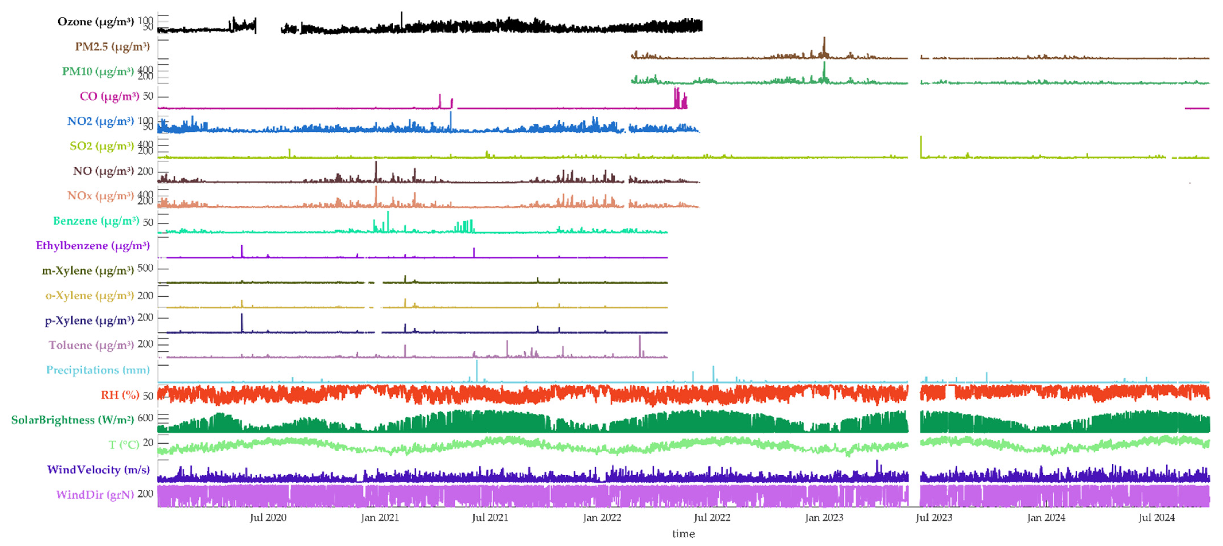
Figure 2 illustrates the temporal distribution of air pollutants and meteorological variables from January 2020 to September 2024, while Figure 3 shows the percentage of missing values by variables. The dataset includes six target pollutants (O₃, PM_2.5, PM₁₀, CO, NO₂, and SO₂) along with a set of predictor variables such as nitrogen oxides (NO, NO_x), volatile organic compounds (benzene, ethylbenzene, xylenes, and toluene), and meteorological parameters (precipitation, relative humidity, solar brightness, temperature, wind velocity, and wind direction). Several discontinuities are observed in the time series, indicating periods of missing data, likely due to sensor downtime or data-acquisition interruptions. Despite these gaps, the time series displays consistent temporal and seasonal behaviour, demonstrating the overall reliability of the monitoring network.

To address missing data, the rmmissing function available in MATLAB 2024a was employed. This function automatically removes entries with missing values from an array or table. Specifically, when applied to a vector, it eliminates any element containing missing data; when applied to a matrix or table, it removes any row that includes missing values.

Clear seasonal and interannual patterns are visible across most pollutants. Ozone concentrations exhibit a distinct annual cycle, with higher levels during summer months, reflecting the role of solar radiation and temperature in photochemical ozone formation. In contrast, PM_2.5 and PM₁₀ show irregular peaks, typically associated with episodic pollution events such as dust intrusions, traffic-related emissions, or biomass burning. Combustion-related pollutants, including CO and NO₂, tend to increase during colder months, reflecting higher fuel consumption and reduced atmospheric dispersion. SO₂ concentrations remain generally low, punctuated by occasional spikes that may indicate localised industrial or heating activities.

The synchronous fluctuations of NO and NO₂ (NO_x) highlight their common origin from vehicular and combustion sources. Volatile organic compounds (VOCs) such as benzene, xylenes, and toluene exhibit similar episodic increases, often aligning with NO_x peaks. This alignment provides strong confirmation of their co-emission from traffic or industrial activities, providing a reliable basis for further research and policy decisions. Conversely, ozone tends to vary inversely with NO_x and VOC levels, consistent with the photochemical titration processes that govern ozone dynamics in urban and suburban environments.

Meteorological parameters also display clear periodic behaviours. Relative humidity (RH) and temperature (T) exhibit inverse seasonal trends, with high RH during cooler months and elevated temperatures in summer. Solar brightness follows the expected annual solar cycle and coincides with the observed ozone peaks, emphasising the importance of radiation in ozone formation. Wind velocity and direction show marked short-term variability, reflecting their role in pollutant dispersion and transport. Sporadic precipitation events are associated with temporary decreases in particulate matter concentrations, suggesting wet deposition and atmospheric cleansing effects.

2.2. AI-Based Modelling Framework

The AI-based modelling framework used to analyse the six major air pollutants builds on the foundation established in our previous study [14]. The methodological approach integrates Machine Learning (ML) and Deep Learning (DL) algorithms explicitly designed for prediction, feature engineering, dimensionality reduction, and time-series forecasting.

For predictive modelling, 23 ML and DL algorithms were implemented, optimised, and compared to determine the most accurate model for each pollutant. The evaluated models include: Artificial Neural Network (ANN), Decision Tree (DT), Support Vector Machine (SVM), Extreme Learning Machine (ELM), Gradient Boosting Machine (GBoost), Extreme Gradient Boosting (xGBoost), Random Forest (RF), Tree Bagger (TreeBag), Generalised Linear Regression (GLR), Gaussian Process Regression (GPR), Linear Regression (LR), Generalised Additive Model (GAM), Kernelised Ridge Regression (KRR), K-Nearest Neighbours (KNN), Linear Ridge Regression (LRR), Bayesian Linear Regression (BayesLR), Convolutional Neural Network (CNN), Feedforward Neural Network (FNN), Deep Neural Network (DNN), Residual Neural Network (ResNet), Fully Connected Neural Network (FCNN), Long Short-Term Memory (LSTM), and LSTM-based Recurrent Neural Network (LSTM-RNN).

The best-performing model from this prediction stage was further integrated with Feature Selection (FS) and SHAP value analysis to identify the most influential predictors, enhancing model interpretability and forecasting accuracy. As detailed in [14], 50 feature selection techniques were compared to identify the most effective variable reduction strategies.

In the final stage, future pollutant concentrations were forecasted using advanced statistical and AI-based time-series models. A Deep Nonlinear Autoregressive Moving Average (Deep-NARMAX) model with Exogenous inputs was implemented to capture nonlinear dependencies between pollutants and meteorological variables, providing a robust framework for multi-step air quality forecasting.

To ensure reproducibility, the forecasting setup is defined as follows:

–

Input Layer: The models utilise a look-back window of past hours of meteorological and pollutant data to capture relationships between them and the target variable. Each target studied here is forecasted alone.

–

Forecasting Horizon: The study evaluates two horizons: one-step (1 h ahead) and multi-step ahead.

–

Multi-step Strategy: The Deep-NARMAX model employs a sliding-window approach, using input data at times (t, t − 1, t − 2, …, t − n) to forecast a horizon of (t + 1) hours for single-step forecasting. For multi-step forecasting, the forecast is extended iteratively to (t + 2) hours and beyond. A recursive strategy is adopted for this purpose, whereby the prediction at (t + 1) is fed back as an input to generate the prediction at (t + 2), and so forth.

2.3. Framework and Evaluation Criteria

2.3.1. Study Framework

Below is the operational framework followed in this study:

• Data ingestion: Import raw data, timestamp normalisation, flag missing values;
• Pre-processing: Remove anomaly and suspect values, gap imputation, outlier handling, resampling;
• Exploratory analysis: Analyse trend, distributions, diurnal/seasonal plots, cross-correlation & causality;
• Data splitting: Divided data into Train/Test subsets (0.7/0.3) using blocked rolling CV + final chronological holdout;
• Prediction Model development: Find candidate models (XGBoost, RF, CNN, LSTM…) → hyperparameter optimisation;
• Feature engineering: Find the best predictors for each air pollutant using various FS techniques, permutation importance, and partial dependence;
• Evaluation and diagnostics: Compute statistical metrics;
• Explainability: Computing SHAP value;
• Forecasting Model development: Find the best formula for each pollutant using Deep-NARMAX architecture;
• Reporting and deployment: produce standardised plots (diurnal/seasonal, heatmaps, SHAP), store models and scalers, prepare for real-time inference.

2.3.2. Evaluation Criteria and Statistical Indices

In this study, a composite statistical evaluation approach based on a performance score (φ) was developed and described to assess the effectiveness of various prediction models—Equation (1). This performance score serves as an integrated metric for ranking and comparing regression models, providing a unified framework for quantifying their predictive accuracy and robustness.

$$\mathrm{\phi }=\mathrm{r}\mathrm{a}\mathrm{n}\mathrm{k}\left(\mathrm{M}\mathrm{B}\mathrm{E}\right)+\mathrm{r}\mathrm{a}\mathrm{n}\mathrm{k}\left(\mathrm{R}\mathrm{M}\mathrm{S}\mathrm{E}\right)+\mathrm{r}\mathrm{a}\mathrm{n}\mathrm{k}\left(\mathrm{M}\mathrm{A}\mathrm{P}\mathrm{E}\right)+\mathrm{r}\mathrm{a}\mathrm{n}\mathrm{k}\left(\mathrm{T}\mathrm{S}\right)+\mathrm{r}\mathrm{a}\mathrm{n}\mathrm{k}\left({\mathrm{R}}^2\right)+\mathrm{r}\mathrm{a}\mathrm{n}\mathrm{k}\left(\mathrm{W}\mathrm{I}\mathrm{A}\right)+\mathrm{r}\mathrm{a}\mathrm{n}\mathrm{k}\left(\mathrm{S}\mathrm{B}\mathrm{F}\right)$$

(1)

where MBE (Mean Bias Error), RMSE (Root Mean Square Error), standard deviation σ and TS (Test Statistic) are known as indicators of dispersion (indicators of error), while R² (Coefficient of Determination), WIA (Willmott’s Index of Agreement) and SBF (Slope of Best-Fit line) are known as indicators of overall performance. Collectively, these metrics provide a comprehensive evaluation of each model’s precision, consistency, and reliability in both prediction and forecasting tasks [15].

Expressions for these metrics are given below:

$$\mathrm{M}\mathrm{B}\mathrm{E}={\displaystyle \frac{1}{\mathrm{K}}}\sum \left({\mathrm{H}}_{\mathrm{p}}^{\mathrm{i}}-{\mathrm{H}}_{\mathrm{m}}^{\mathrm{i}}\right)$$

(2)

$$\mathrm{R}\mathrm{M}\mathrm{S}\mathrm{E}={\left({\displaystyle \frac{1}{\mathrm{K}}}\sum {\left({\mathrm{H}}_{\mathrm{p}}^{\mathrm{i}}-{\mathrm{H}}_{\mathrm{m}}^{\mathrm{i}}\right)}^2\right)}^{{\displaystyle \frac{1}{2}}}$$

(3)

$$\mathrm{M}\mathrm{A}\mathrm{P}\mathrm{E}={\displaystyle \frac{100}{\mathrm{K}}}\sum \left|{\displaystyle \frac{\left({\mathrm{H}}_{\mathrm{p}}^{\mathrm{i}}-{\mathrm{H}}_{\mathrm{m}}^{\mathrm{i}}\right)}{{\mathrm{H}}_{\mathrm{m}}^{\mathrm{i}}}}\right|$$

(4)

$$\mathrm{T}\mathrm{S}={\left[{\displaystyle \frac{\left(\mathrm{K}-1\right){\mathrm{M}\mathrm{B}\mathrm{E}}^2}{\left({\mathrm{R}\mathrm{M}\mathrm{S}\mathrm{E}}^2-{\mathrm{M}\mathrm{B}\mathrm{E}}^2\right)}}\right]}^{1/2}$$

(5)

$$\mathsf{\sigma }={\left[{\displaystyle \frac{\mathrm{K}\left({\mathrm{R}\mathrm{M}\mathrm{S}\mathrm{E}}^2-{\mathrm{M}\mathrm{B}\mathrm{E}}^2\right)}{\left(\mathrm{K}-1\right)}}\right]}^{1/2}$$

(6)

$${\mathrm{R}}^2=1-{\displaystyle \frac{\sum {\left({\mathrm{H}}_{\mathrm{p}}^{\mathrm{i}}-{\mathrm{H}}_{\mathrm{m}}^{\mathrm{i}}\right)}^2}{\sum {\left({\mathrm{H}}_{\mathrm{m}}^{\mathrm{i}}-\overline{{\mathrm{H}}_{\mathrm{m}}}\right)}^2}}$$

(7)

$$\mathrm{S}\mathrm{B}\mathrm{F}={\displaystyle \frac{\left[\sum \left({\mathrm{H}}_{\mathrm{p}}^{\mathrm{i}}-\overline{{\mathrm{H}}_{\mathrm{p}}}\right)\left({\mathrm{H}}_{\mathrm{m}}^{\mathrm{i}}-\overline{{\mathrm{H}}_{\mathrm{m}}}\right)\right]}{\sum {\left({\mathrm{H}}_{\mathrm{m}}^{\mathrm{i}}-\overline{{\mathrm{H}}_{\mathrm{m}}}\right)}^2}}$$

(8)

$$\mathrm{W}\mathrm{I}\mathrm{A}=1-{\displaystyle \frac{\left[\sum {\left({\mathrm{H}}_{\mathrm{p}}^{\mathrm{i}}-{\mathrm{H}}_{\mathrm{m}}^{\mathrm{i}}\right)}^2\right]}{\sum {\left[\left|{\mathrm{H}}_{\mathrm{p}}^{\mathrm{i}}-\overline{{\mathrm{H}}_{\mathrm{m}}}\right|+\left|{\mathrm{H}}_{\mathrm{m}}^{\mathrm{i}}-\overline{{\mathrm{H}}_{\mathrm{m}}}\right|\right]}^2}}$$

(9)

where K is the total number of observations; ${\mathrm{H}}_{\mathrm{p}}^{\mathrm{i}}$, ${\mathrm{H}}_{\mathrm{m}}^{\mathrm{i}}$ and $\overline{\mathrm{H}}$ are the ith predicted value, ith measured value and mean value, respectively.

3. Results and Discussion

3.1. Temporal Variability of Air Pollutants

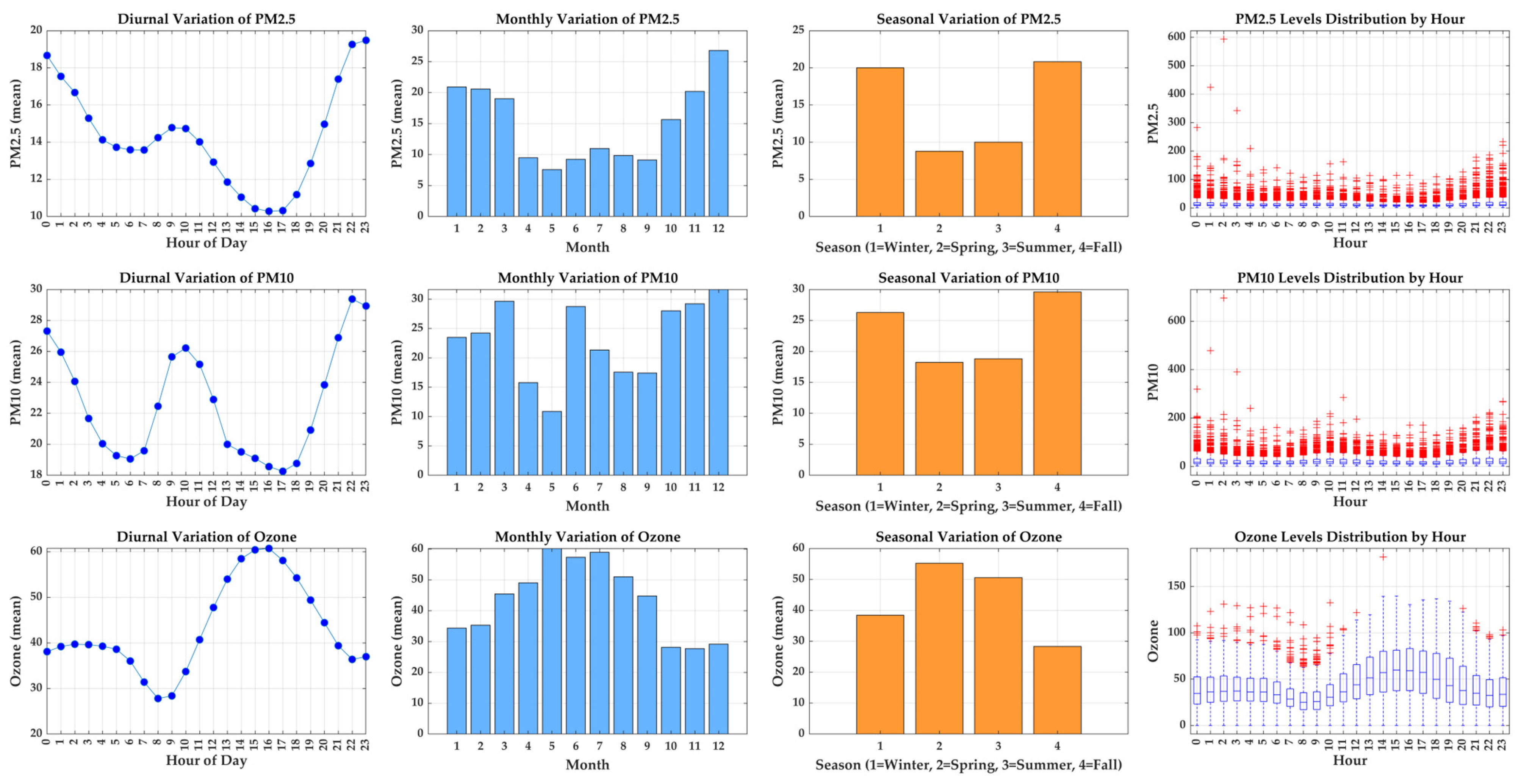
Figure 4 presents the diurnal, monthly, and seasonal variations in PM_2.5, PM₁₀, and O₃ concentrations, together with their hourly distribution profiles. Distinct temporal patterns are evident for each pollutant, reflecting differences in emission sources, atmospheric processes, and meteorological influences.

The diurnal variation in PM_2.5 exhibits two pronounced peaks: one during the early morning hours and another at night, with a minimum in the afternoon. Traffic emissions, domestic heating, and limited atmospheric dispersion during stable nocturnal conditions primarily drive this behaviour. The afternoon minimum corresponds to enhanced mixing and dilution due to solar heating and stronger winds. Similarly, PM₁₀ shows a bimodal diurnal pattern, consistent with the accumulation of coarse particles from traffic, resuspension, and local emissions during morning and evening rush hours.

On a monthly and seasonal scale, both PM_2.5 and PM₁₀ concentrations are highest during winter and fall and lowest during summer. This seasonal pattern can be attributed to the combined effects of increased combustion sources in colder months, weaker vertical mixing, and frequent temperature inversions that trap pollutants near the surface. Conversely, higher summer temperatures and stronger atmospheric circulation promote particle dispersion and removal, resulting in lower particulate matter levels.

In contrast, ozone (O₃) exhibits an inverse temporal behaviour. The diurnal variation shows a typical photochemical pattern, with low concentrations in the early morning and a clear peak in the afternoon (around 14:00–16:00), coinciding with maximum solar radiation and photochemical activity. Ozone levels decrease again in the evening due to titration with nitrogen oxides and reduced photochemical production. On a seasonal basis, ozone reaches its maximum during spring and summer, reflecting enhanced sunlight intensity, higher temperatures, and favourable photochemical conditions for ozone formation, whereas winter values remain significantly lower.

The hourly boxplots further highlight variability in pollutant levels, showing greater dispersion and occasional high outliers at night for PM_2.5 and PM₁₀, and in the afternoon for ozone. These outliers represent pollution episodes likely driven by local emission peaks or specific meteorological conditions.

Figure 5 illustrates the diurnal, monthly, and seasonal variations of carbon monoxide (CO), sulphur dioxide (SO₂), and nitrogen dioxide (NO₂) concentrations, along with their hourly distributions. These pollutants are strongly linked to combustion sources such as vehicular traffic, industrial activities, and domestic heating, as reflected in their temporal patterns.

The diurnal variation in CO shows an early-morning minimum, followed by a steady increase throughout the day, peaking in the late evening. This pattern suggests that CO accumulation is influenced by both rush-hour traffic and reduced atmospheric dispersion during nighttime. The monthly and seasonal analyses indicate that CO levels peak in spring, with markedly lower concentrations in summer. Springtime enhancement could be linked to a combination of residual heating emissions, local meteorological stagnation, and potential long-range transport episodes.

For SO₂, the diurnal pattern exhibits a pronounced daytime peak around midday, following a nighttime minimum. This increase coincides with the onset of industrial and domestic activities and with vertical mixing of pollutants after sunrise. Monthly, SO₂ concentrations remain relatively stable, showing only slight increases during colder months. Seasonally, the pollutant maintains high and nearly constant levels across winter, spring, and fall, which may indicate continuous background emissions from traffic, industrial, or residential combustion sources.

The NO₂ time series displays a classic bimodal diurnal structure, characterised by morning and evening peaks, coinciding with peak vehicular traffic, and a distinct midday trough associated with photochemical reactions that convert NO₂ into ozone under intense sunlight. Monthly and seasonal trends show elevated NO₂ levels in winter and fall, with levels declining in spring and reaching minimum values in summer. These variations result from increased heating and transport emissions, reduced atmospheric mixing in cold months, and enhanced photochemical removal during warm, sunny periods.

The hourly boxplots further emphasise the variability of each pollutant, showing larger ranges and more pronounced outliers during the morning and evening hours for NO₂ and CO, while SO₂ displays occasional extreme values that may be linked to short-term industrial or emission spikes.

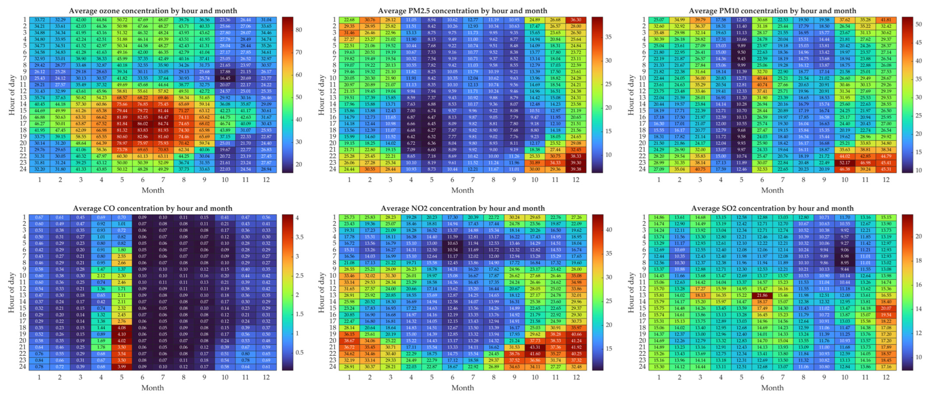
Figure 6 presents the hourly and monthly mean concentrations of the six key pollutants—PM_2.5, PM₁₀, O₃, CO, NO₂ and SO₂—highlighting their distinct temporal signatures across different months and times of day.

The ozone distribution shows a pronounced daytime maximum, peaking around midday to early afternoon (11:00–16:00), especially during late spring and summer months (May–August). This pattern aligns with enhanced photochemical production under intense solar radiation and higher temperatures. Conversely, nighttime ozone levels remain low due to titration with nitrogen oxides. Both PM_2.5 and PM₁₀ exhibit elevated concentrations during winter and early spring, with notable peaks in December–March and reduced levels in summer. Their diurnal cycles are relatively stable but tend to rise during morning and evening hours, reflecting local emission sources (traffic, domestic heating) and limited boundary-layer mixing under colder conditions. CO shows evident seasonal variability, with high concentrations in spring and winter and low levels in summer. Its diurnal profile shows late-evening maxima, consistent with traffic activity and reduced nighttime dispersion. NO₂ displays a typical bimodal pattern, characterised by peaks during morning and evening rush hours and minima around midday when photochemical conversion to ozone is strongest. Higher values during winter and fall confirm the strong dependence of NO₂ on combustion emissions and atmospheric stability. Finally, SO₂ concentrations remain relatively moderate throughout the year but show slight increases during winter and fall, likely associated with domestic heating and lower atmospheric mixing heights. Diurnal variation is modest, with minor increases at midday linked to industrial and traffic-related emissions.

3.2. Cross-Correlation Analysis

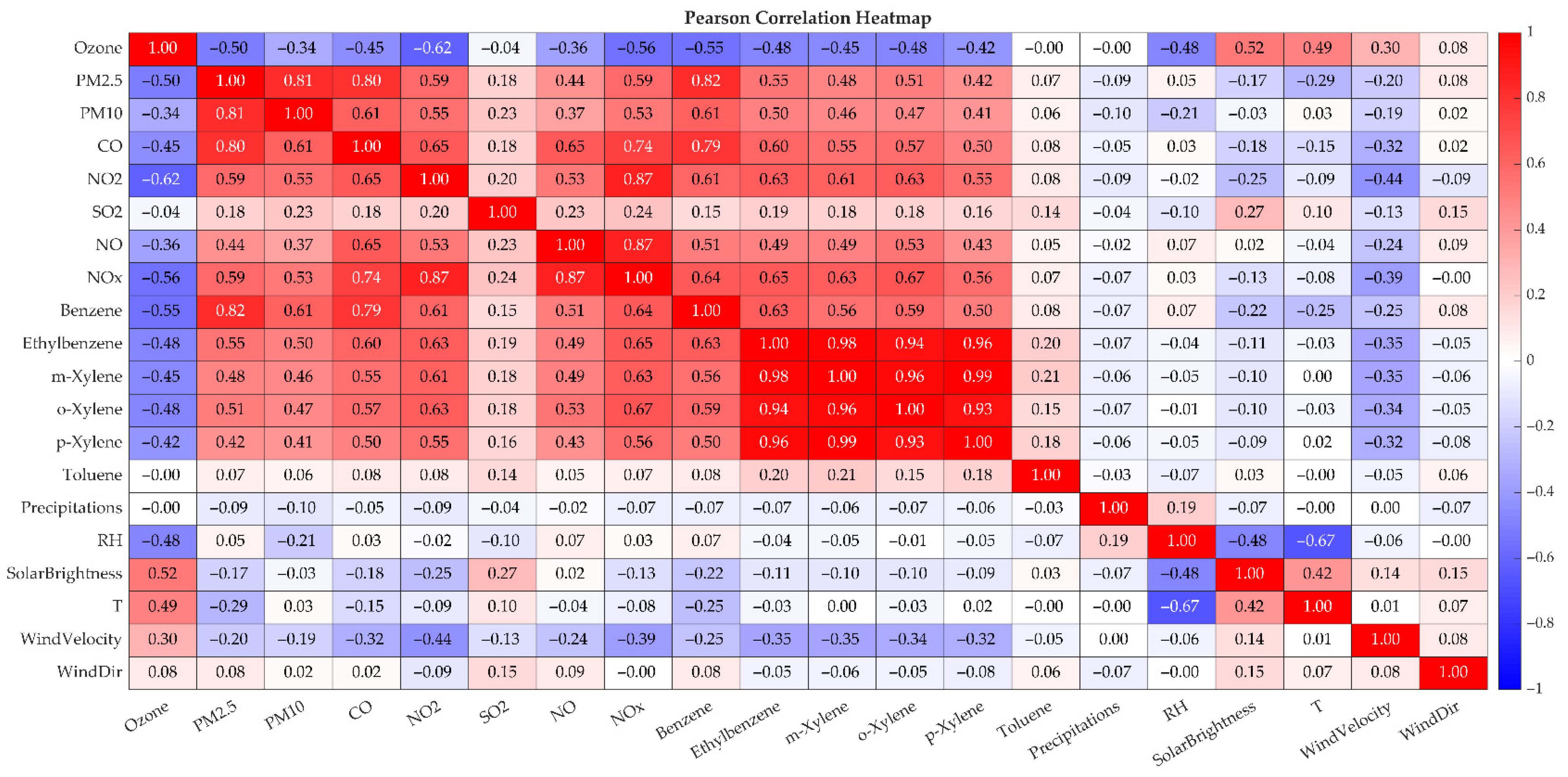
Cross-correlation analysis measures the similarity between two time series as a function of their relative displacement. This method assesses the direction and strength of linear correlations between the air pollutants under study and the influencing variables, as well as the time lags at which these relationships are strongest [16]. Figure 7 illustrates the Pearson correlation coefficients among the pollutants (PM_2.5, PM₁₀, O₃, CO, NO₂, SO₂) and the set of meteorological and gaseous predictor variables. Several notable patterns emerge, revealing both direct and inverse dependencies that highlight the interplay between primary emissions, secondary formation, and meteorological influence. The ozone (O₃) concentration shows strong negative correlations with NO₂ (r = −0.62), NO_x (r = −0.56), and CO (r = −0.45), indicating that high levels of primary pollutants coincide with reduced ozone due to titration reactions and limited photochemical production. This inverse relationship is consistent with the NO titration effect observed in high-traffic urban environments, where fresh nitric oxide (NO) emissions scavenge ozone (NO + O₃ → NO₂ + O₂), particularly during periods of low solar radiation or high vehicle activity. Conversely, ozone is positively correlated with solar brightness (r = 0.52) and temperature (r = 0.49), confirming the role of photochemical activity under intense solar radiation and warm conditions. Particulate matter (PM_2.5 and PM₁₀) exhibits a strong mutual correlation (r = 0.81), confirming their shared sources and atmospheric behaviour. Both pollutants correlate highly with CO (r = 0.80 and 0.61), NO₂ (r = 0.59 and 0.55), suggesting that they originate from traffic and combustion emissions. Additionally, PM_2.5 exhibits a robust correlation with benzene (r = 0.82) and other aromatic hydrocarbons, suggesting that fine particulate pollution is linked to volatile organic compound (VOC) emissions. The relationship between CO and NO₂ is also strong (r = 0.65), consistent with their common vehicular source. Meanwhile, SO₂ shows only weak to moderate correlations with most pollutants (maximum r = 0.24 with NO₂), implying distinct or more sporadic emission sources, such as industrial and domestic fuel combustion. Meteorological variables show expected influences: relative humidity (RH) is inversely correlated with ozone (r = −0.48) and temperature (r = −0.67), whereas solar brightness is positively associated with temperature (r = 0.42) and inversely with PM_2.5 and PM₁₀. These relationships highlight how meteorological conditions regulate pollutant dispersion and secondary formation processes.

3.3. Granger Causality Tests

A statistical hypothesis test called Granger causality is used to determine if one time series can accurately predict another [17]. To determine whether historical values of meteorological and other air variables can significantly predict future pollution, and vice versa, this study will employ Granger causality tests. This test helps identify directional relationships between variables, providing insights into potential causal influences.

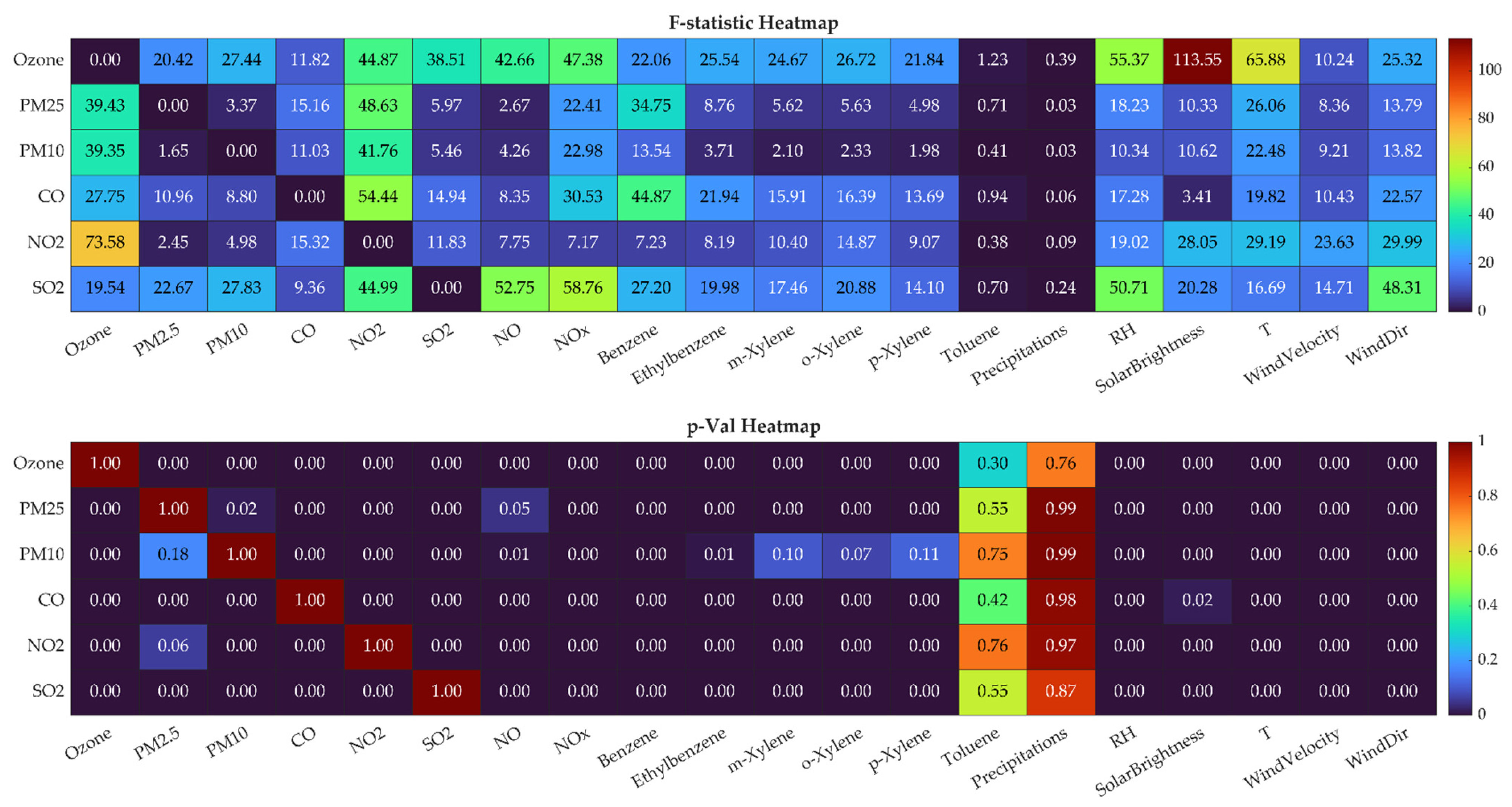
Figure 8 and

Table 3. Granger Causality Summary.

Target Variable	Significant Predictors (p-Val < 0.05 and F-Statistic > 15)	Most Influential (p = 0)	Brief Interpretation
Ozone	PM2.5, PM10, NO2, SO2, NO, NOx, Benzene, Ethylbenzene, m-Xylene, o-Xylene, p-Xylene, RH, Solar Brightness, T, Wind direction	Solar Brightness (p = 0.0000, F = 113.55) and T (p = 0.0000, F = 65.88)	O3 is strongly controlled by temperature and Solar Brightness.
PM2.5	O3, CO, NO2, NOx, Benzene, RH, T	NO2 (p = 0.0000, F = 48.63) and O3 (p = 0.0000, F = 39.43)	Photochemical and nitrogen-based pollutants drive fine-particle formation; meteorological factors also contribute to it.
PM10	O3, NO2, NOx, T	NO2 (p = 0.0000, F = 41.76) and O3 (p = 0.0000, F = 39.35)	Oxidant chemistry and gas-phase precursors influence the dynamics of coarse particles.
CO	O3, NO2, NOx, Benzene, Ethylbenzene, m-Xylene, o-Xylene, RH, T, Wind direction	NO2 (p = 0.0000, F = 54.44) and Benzene (p = 0.0000, F = 44.87)	Traffic-related species and aromatics modulate CO temporal behaviour.
NO2	O3, CO, RH, Solar Brightness, T, Wind velocity, Wind direction	O3 (p = 0.0000, F = 73.58)	Photochemical oxidation and pressure/meteorology affect NO2 variability.
SO2	O3, PM2.5, PM10, NO2, NO, NOx, Benzene, Ethylbenzene, m-Xylene, o-Xylene, RH, Solar Brightness, T, Wind direction	NOx (p = 0.0000, F = 58.76) and NO (p = 0.0000, F = 52.75)	Sulphur oxide levels are linked to combustion, nitrogen oxides, humidity, and transport.

present the results of the Granger causality test among the pollutants studied and their predictor variables, expressed as F-statistic and p-value heatmaps. This analysis identifies potential directional (causal) influences between pollutants and influencing factors, revealing both short-term and lagged interdependencies that go beyond simple correlation.

The F-statistic heatmap (top panel) highlights several statistically significant causal relationships. Among the pollutants, NO₂ appears to exert a strong causal effect on ozone (F = 73.58, p < 0.001), reflecting the well-known photochemical titration effect, in which NO₂ and NO participate in ozone formation and depletion cycles. Similarly, NO₂ has significant effects on CO (F = 44.87) and PM_2.5 (F = 34.75), suggesting that vehicular and combustion emissions contribute simultaneously to both particulate and gaseous pollutants.

Meteorological variables also show significant causal effects on pollutant levels. Solar brightness and temperature strongly influence ozone (F = 113.55 and 65.88, both with p < 0.001), underscoring the role of photochemical activity and thermal enhancement in ozone formation. Conversely, relative humidity (RH) exerts a negative causal influence on ozone (F = 55.37, p < 0.001), suggesting that it reduces photochemical efficiency by increasing cloud cover and moisture.

The p-value heatmap (bottom panel) confirms these relationships, indicating that most causal links between pollutants and meteorological variables are statistically significant at the 95% confidence level (p < 0.05). Notably, insignificant relationships (p > 0.05) are observed between ozone and precipitation, or between ozone and toluene, indicating weaker short-term dynamic links with these variables.

Overall, the Granger causality analysis reveals that ozone dynamics are primarily governed by NO₂, solar brightness, and temperature, while NO₂-related traffic emissions mainly influence PM and CO concentrations. These findings reinforce the conclusion that photochemical and combustion processes jointly drive the temporal evolution of air pollutants, validating their inclusion as predictors in subsequent modelling and forecasting frameworks.

3.4. Temporal Evolution of the Air Quality Index (AQI)

In this subsection, air quality is analysed using the computed Air Quality Index (AQI) for the six major pollutants. According to the World Health Organisation (WHO) guidelines, the overall air quality level is determined by the maximum AQI value among pollutants, which serves as a representative indicator of the general air quality.

While this approach is widely adopted, it inherently overlooks pollutant-specific health impacts. We argue that air quality should ideally be assessed individually for each pollutant, as the dominant pollutant may not always reflect the cumulative or differential exposure risks. This perspective might be further explored in future studies.

In the present work, however, we adhere to the WHO-recommended methodology by first computing the AQI for each pollutant and then identifying the maximum index value to categorise air quality into the standard classes: Good, Moderate, Unhealthy for Sensitive Groups, Unhealthy, Very Unhealthy, and Hazardous. The detailed classification thresholds and pollutant-specific requirements are summarised in

Table 4. U.S. EPA AQI Breakpoints (in µg/m³) ** [18,19].

AQI Category	AQI Range	PM2.5 (24 h)	PM10 (24 h)	O3 (8 h)	CO (8 h)	SO2 (1 h)	NO2 (1 h)
Good	0–50	0.0–9.0	0–54	0–107.9	0–5039	0–91.7	0–99.6
Moderate	51–100	9.1–35.4	55–154	108.0–137.2	5040–10,763	91.8–196.5	99.7–188.0
Unhealthy for Sensitive Groups	101–150	35.5–55.4	155–254	137.3–166.6	10,764–14,198	196.6–484.7	188.1–676.8
Unhealthy	151–200	55.5–125.4	255–354	166.7–205.8	14,199–17,633	484.8–796.5	676.9–1220.1
Very Unhealthy	201–300	125.5–225.4	355–424	205.9–392.0	17,634–34,808	796.6–1582.5	1220.2–2348.1
Hazardous	301–400	225.5–350.4	425–504	-	34,809–46,258	1582.6–2106.5	2348.2–3852.1
Hazardous	401–500	350.5–500.4	505–604	-	46,259–57,708	2106.6–2629.0	3852.2–4757.1
Good	0–50	0.0–9.0	0–54	0–107.9	0–5039	0–91.7	0–99.6
Moderate	51–100	9.1–35.4	55–154	108.0–137.2	5040–10,763	91.8–196.5	99.7–188.0

** Note: SO₂ and NO₂ breakpoints were converted from ppb using 1 ppb SO₂ = 2.62 µg/m³ and 1 ppb NO₂ = 1.88 µg/m³. The EPA AQI calculation for these gases officially uses the ppb values, so using these converted µg/m³ values may introduce minor rounding discrepancies.

.

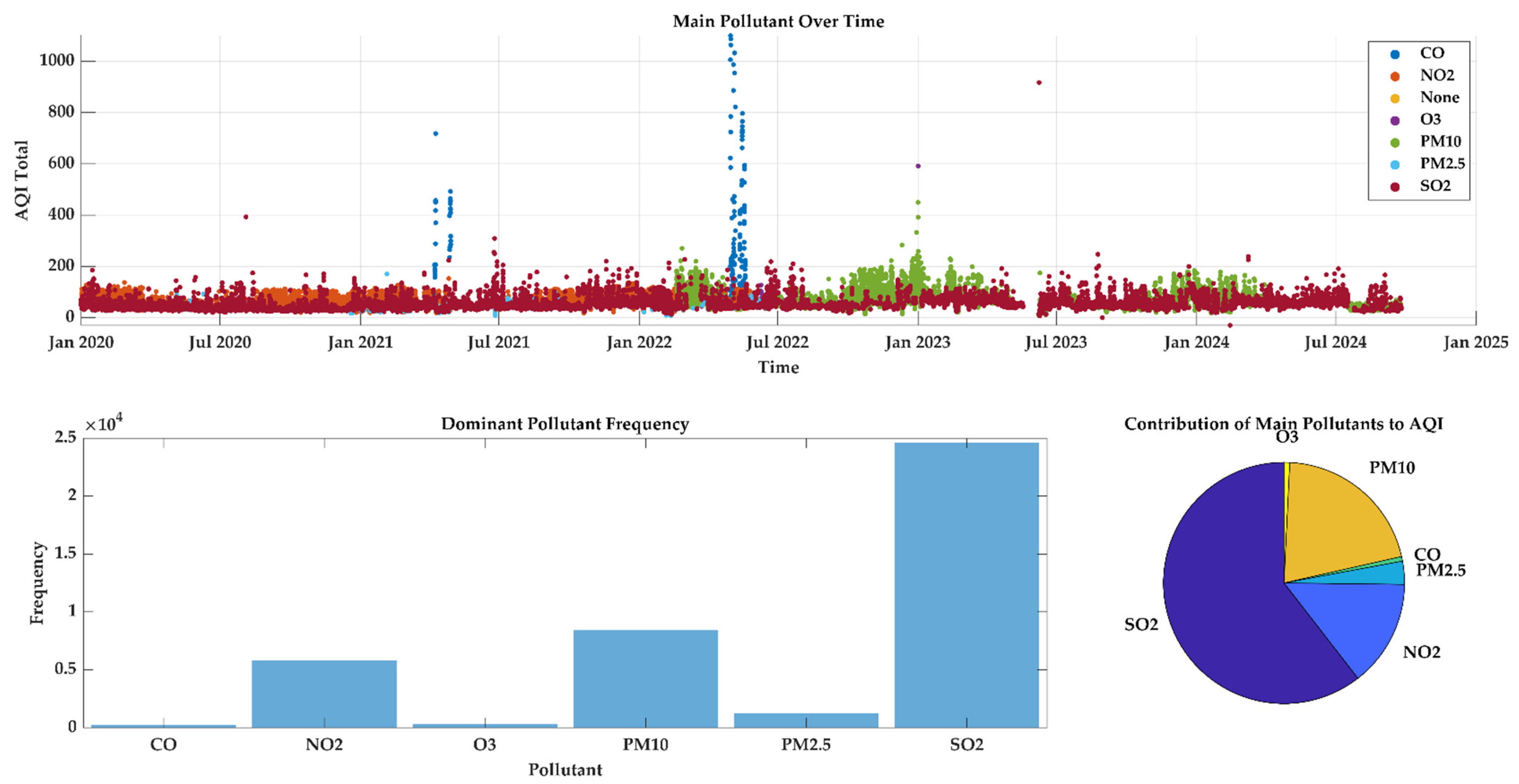
The upper panel (Figure 9) illustrates the evolution of the total AQI, the maximum AQI among the six pollutants, from January 2020 to September 2024, highlighting the dominant pollutant at each point in time. Overall, the AQI fluctuates within low to moderate levels for most of the study period, suggesting generally acceptable air quality with occasional pollution peaks. A notable spike is observed during mid-2022, where AQI values exceeded 1000, primarily driven by CO, indicating an episode of severe air pollution likely associated with either a local emission event (e.g., combustion, traffic congestion, or industrial release) or meteorological stagnation. Periods dominated by SO₂ and PM₁₀ are recurrent, especially during winter and spring, when atmospheric conditions typically favour pollutant accumulation.

The lower-left panel presents the frequency of dominance among the six major pollutants. The analysis reveals that SO₂ overwhelmingly dominates the AQI contribution, accounting for the highest frequency of exceedances, followed by PM₁₀ and NO₂. This pattern suggests that industrial emissions and vehicular exhaust remain the primary drivers of air quality degradation in the region. The lower frequencies of CO, O₃, and PM_2.5 indicate that these pollutants, while important, play a secondary role in determining daily AQI dominance.

The pie chart on the lower right quantifies the relative contributions of the primary pollutants to the total AQI. SO₂ is the leading contributor, accounting for more than half of the total AQI burden. PM₁₀ and NO₂ follow with moderate shares, reflecting the combined effects of vehicular traffic, industrial activities, and resuspended dust. In contrast, CO and PM_2.5 contribute minimally, and O₃ plays a relatively minor role during the analysed period. This distribution indicates that primary pollutants—particularly those directly emitted from combustion sources—dominate over secondary pollutants such as ozone.

Collectively, Figure 9 underscores that the air quality in the study area is primarily influenced by SO₂, PM₁₀, and NO₂, with occasional severe pollution episodes linked to CO spikes. The dominance of these pollutants underscores the need for targeted emission control strategies focused on fuel quality, industrial desulphurisation, and particulate matter abatement. Moreover, the observed temporal variations highlight the influence of seasonal meteorology and anthropogenic activities on pollutant dynamics.

3.5. Best AI-Based Predicting Models

Table 5. A statistical analysis of the best AI-based model in predicting each of the six pollutants.

Stage	Variable	AI-Based Model	R2	MBE	MAE	RMSE	MAPE	σ
Training	PM2.5	xGBoost	0.991	−1.58 × 10−8	1.801	2.477	0.185	2.478
	PM10	xGBoost	0.986	−2.85 × 10−8	4.289	6.046	0.440	6.049
	Ozone	Random Forest	0.964	−0.014	4.827	6.690	0.040	6.690
	CO	xGBoost	0.950	−1.97 × 10−10	0.154	0.518	0.001	0.518
	NO2	CNN	0.999	0.134	0.210	0.504	0.001	0.485
	SO2	Random Forest	0.874	0.010	1.675	4.146	0.013	4.146
Testing	PM2.5	xGBoost	0.897	−0.007	6.032	10.995	1.446	11.009
	PM10	xGBoost	0.791	−0.483	12.136	19.454	2.910	19.472
	Ozone	Random Forest	0.888	−0.004	8.0121	10.821	0.157	10.822
	CO	xGBoost	0.639	−0.004	0.216	1.123	0.004	1.123
	NO2	CNN	0.999	0.120	0.218	0.662	0.003	0.651
	SO2	Random Forest	0.407	0.042	2.891	7.198	0.052	7.199

summarises the statistical performance of the best-performing AI-based models for each pollutant during training and testing. The results demonstrate the high predictive accuracy and generalisation capability of the selected models across all pollutants, albeit with varying degrees of robustness.

For PM_2.5 and PM₁₀, the XGBoost model achieved outstanding performance during training (R² = 0.99 and 0.99, respectively) and maintained high accuracy during testing (R² = 0.90 for PM_2.5; R² = 0.79 for PM₁₀). Despite slight performance degradation during testing, the results confirm the model’s strong ability to capture particulate dynamics driven by complex nonlinear interactions among VOCs and meteorological variables.

Ozone (O₃) and sulphur dioxide (SO₂) were best predicted by Random Forest models, achieving R² = 0.96 and 0.87 during training, and 0.89 and 0.41 during testing, respectively. The relatively lower testing correlation for SO₂ reflects its more episodic and source-dependent nature, which can limit model generalisation.

Carbon monoxide (CO) prediction using XGBoost yielded R² = 0.95 on training and 0.64 in testing, suggesting that CO variability is influenced by highly transient emission patterns, such as traffic intensity.

Finally, nitrogen dioxide (NO₂), modelled using a Convolutional Neural Network (CNN), showed exceptional predictive stability with R² values above 0.99 for both phases and minimal errors (RMSE < 0.7 µg/m³), highlighting the CNN’s capability to learn spatiotemporal features effectively.

Overall, these findings confirm that ensemble-based (XGBoost, Random Forest) and deep learning (CNN) architectures outperform conventional models, demonstrating their suitability for nonlinear air quality prediction tasks and providing a robust foundation for further deployment in real-time forecasting systems.

Table 6. Performance Comparison with Recent Multivariate Air Pollution Prediction Studies.

Study (Ref)	Model Architecture	Horizon	Target	R2	RMSE
Li et al. [20]	Residual Nested LSTM (NLSTM) + DSWT (wavelet)	Hourly	PM2.5	0.96	27.56
			PM10	0.94	32.93
			O3	0.92	7.17
			CO	0.94	584.0
			NO2	0.89	6.93
			SO2	0.89	7.12
Havaei et al. [21]	Multi-timescale Attention Neural ODE (MA-NODE)	Daily	PM2.5	0.953	2.716
			PM10	0.949	7.001
			O3	0.957	2.020
			CO	0.929	0.157
			NO2	0.946	3.366
			SO2	0.903	0.673
Narmeen Fatima et al. [22]	Kalman-Attention BiGRU	Hourly	PM2.5	0.957	0.166
			PM10	0.960	0.208
			O3	0.93	0.004
			CO	0.937	0.005
			NO2	0.937	0.003
			SO2	0.665	6.41 × 10−4
Dey [23]	CNN + Stacked LSTM (C2SLSTM)	Hourly	PM2.5	0.804	0.288
			CO	0.807	0.290
			NO2	0.91	0.288
Yuan et al. [9]	CNN-LSTM + Attention	Hourly	O3	0.971	3.59
Ihsan Uluocak et al. [24]	Hybrid CNN-LSTM and CNN-GRU	Daily	NO2	From 0.920 to 0.955	From 0.244 to 0.269

summarises performance comparison with recent multivariate air pollution prediction studies between 2020 and 2025.

3.6. Shapley Additive Explanations

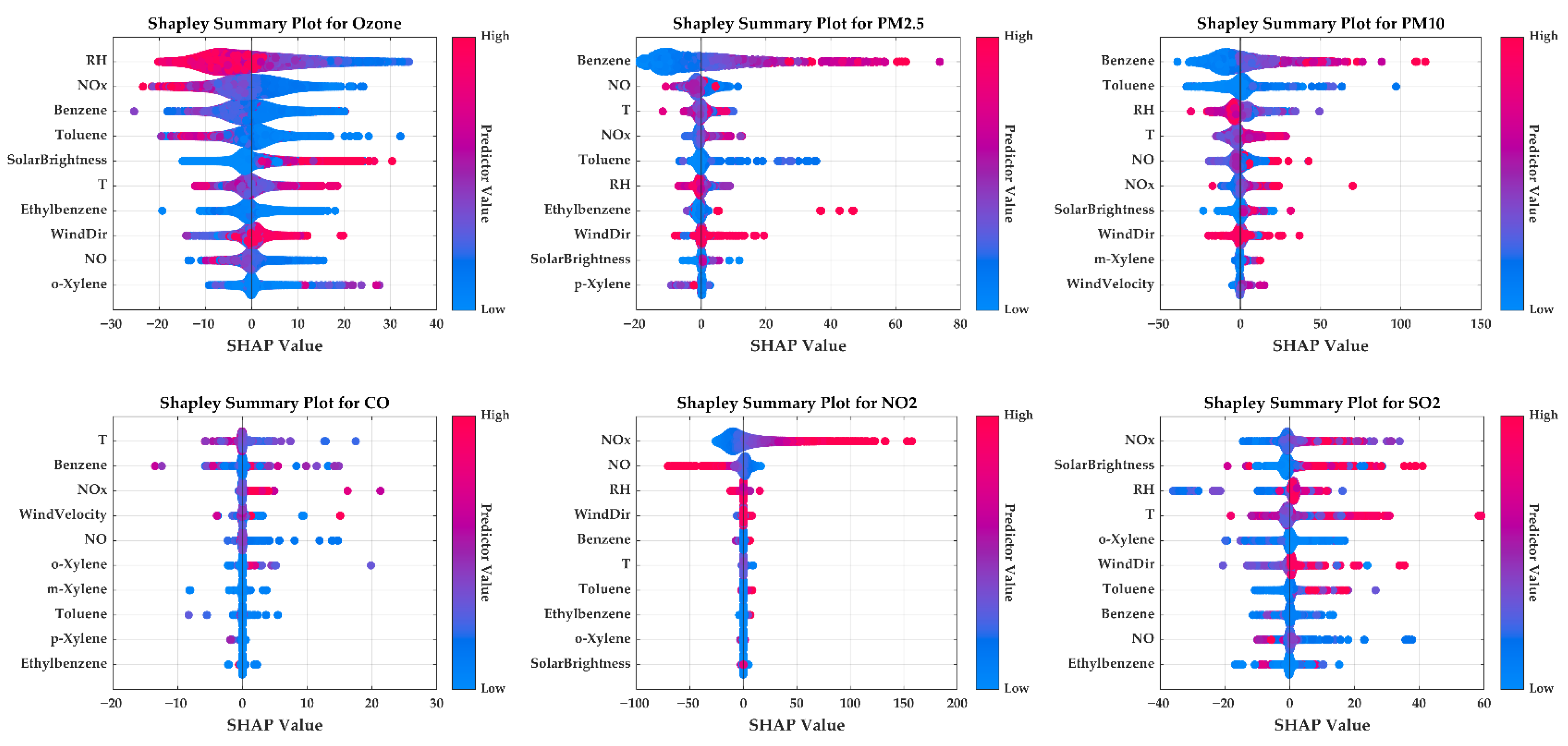
Figure 10 illustrates the Shapley Additive Explanations (SHAP) results for the six pollutants, highlighting the most influential meteorological and chemical predictors affecting their concentrations. For ozone (O₃), relative humidity (RH), NO_x, solar brightness, and temperature are the dominant variables. High RH and NO_x exhibit negative SHAP values, indicating ozone suppression under humid or NO-rich conditions, whereas intense solar radiation and elevated temperatures enhance photochemical ozone formation.

For PM_2.5 and PM₁₀, benzene, toluene, NO₂ and NO are the main predictors, reflecting the role of combustion-related VOCs and nitrogen oxides in secondary particle formation. High VOC levels contribute positively to particulate accumulation, while humidity has a moderate positive effect, especially on PM₁₀, due to hygroscopic growth. In the case of carbon monoxide (CO), temperature, benzene, and NO_x exert the most significant influence, indicating a strong link between CO levels and vehicular emissions. For nitrogen dioxide (NO₂), NO dominates, reflecting direct chemical coupling, whereas RH reduces NO₂ through wet deposition. For sulphur dioxide (SO₂), the most influential variables are NO_x, solar brightness, RH, and temperature: dry, sunny conditions enhance concentrations, whereas high humidity promotes SO₂ removal.

Overall, SHAP results confirm that NO_x, VOCs (benzene, toluene, xylenes), and key meteorological factors (RH, temperature, solar brightness) consistently drive pollutant behaviour, underscoring the intertwined effects of emission sources and atmospheric processes on air quality dynamics.

3.7. Feature Selection

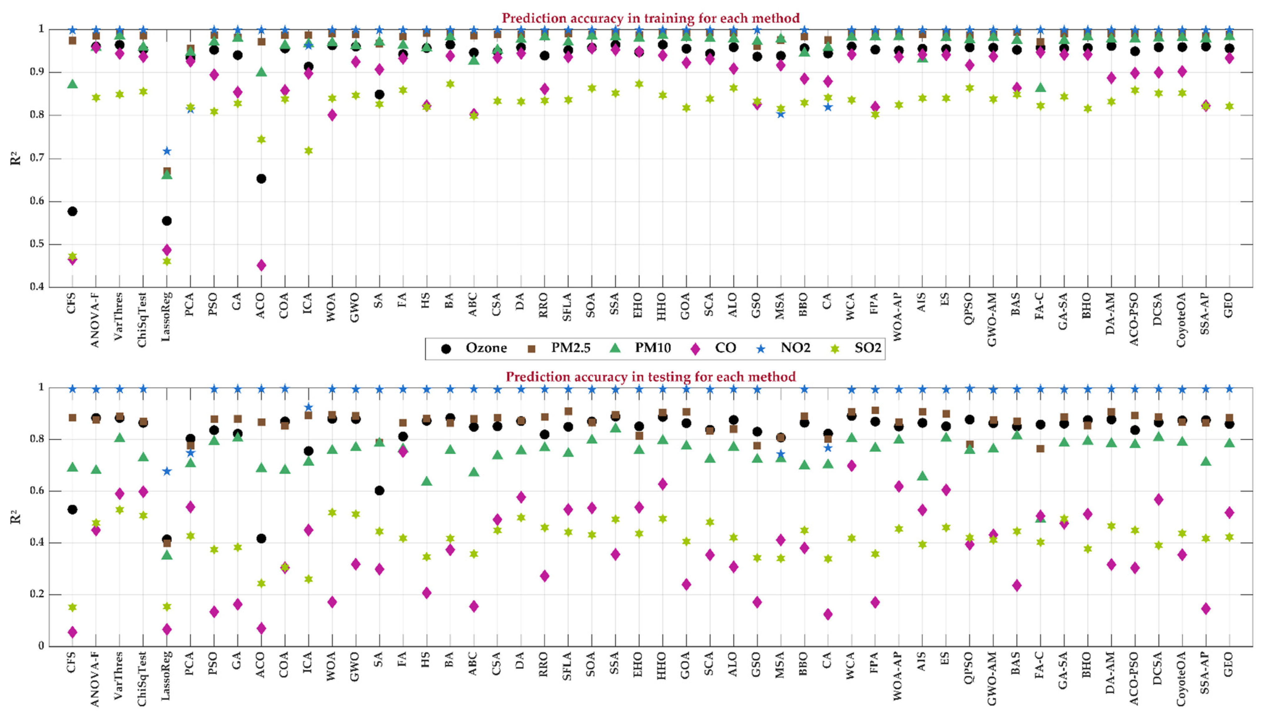
Figure 11 summarises the best features selected by each of the fifty-feature section (FS) methods. Figure 12 presents a comprehensive statistical comparison of the prediction accuracy achieved by the hybrid AI-based FS framework across all evaluated methods for the six pollutants. This is performed for both training and testing stages.

The figure displays the R² values for both training and testing phases, allowing a clear assessment of the robustness, generalisation, and stability of each FS technique when coupled with the predicting model. The results highlight substantial variability in predictive performance across methods, confirming that FS directly and significantly influences model prediction accuracy.

During the training phase, most FS techniques yield strong predictive behaviour for O₃, PM_2.5, PM₁₀, CO, and NO₂, with R² values generally exceeding 0.85. This result indicates that the hybrid AI–FS architecture successfully captures the intrinsic structure and nonlinear relationships within the high-dimensional dataset. Some traditional methods, such as CFS, ANOVA-F, Chi-square Test, and LassoReg, show moderate performance, while most bio-inspired and swarm-intelligence-based optimisers—such as PSO, GA, GWO, HHO, and SSA—achieve consistently higher R² values, often approaching or exceeding 0.95 for specific pollutants. The elevated clustering of points near the top of the training plot reflects the ability of these optimisers to search the feature space and efficiently identify informative subsets.

In contrast, the testing phase (bottom panel) reveals greater variability across methods, providing more insight into their generalisation capability and susceptibility to overfitting. While pollutants such as O₃, PM_2.5, and NO₂ maintain high predictive quality—with many methods sustaining R² values above 0.80—the performance for CO, PM₁₀, and especially SO₂ shows more dispersed patterns. This behaviour highlights the increased difficulty of modelling pollutants with irregular emissions or episodic fluctuations. Notably, some FS techniques that perform well during training (e.g., ACO, BA, and CSA) show a clear drop in testing accuracy, suggesting potential overfitting. Conversely, methods such as PSO, GA, GWO-AM, and several adaptive or hybrid metaheuristics demonstrate superior stability, preserving high R² values during testing across pollutants.

A recurring trend is the comparatively lower accuracy for SO₂ across nearly all FS methods, with many testing R² values falling between 0.20 and 0.50. This finding aligns with the pollutant-specific results from the prediction analysis. It reinforces the notion that SO₂ exhibits highly irregular, source-dependent behaviour that is less predictable through data-driven approaches alone. On the other hand, the consistently high performance for NO₂, with many FS techniques achieving R² ≈ 1 during both training and testing, illustrates a strong and stable relationship between NO₂ variability and the selected explanatory variables.

Table 7. A summary of the best hybrid AI-based FS model for each pollutant.

Variable	Stage	FS Algorithm	R2	MBE	MAE	RMSE	MAPE	Sd	Predictors
Ozone	Training	DA-AM	0.961	−0.003	4.981	6.889	0.042	6.889	NO, NO2, Benzene, Ethylbenzene, o-Xylene, RH, SolarBrightness, T, WindVelocity, and WindDir
	Testing	SSA	0.889	−0.036	8.1251	10.983	0.160	10.984	NO, NO2, Benzene, Ethylbenzene, m-Xylene, o-Xylene, p-Xylene, Toluene, Precipitations, RH, SolarBrightness, T, WindVelocity, and WindDir
PM2.5	Training	WOA-AP	0.992	−1.57 × 10−8	1.777	2.466	0.182	2.468	NO, NO2, Benzene, o-Xylene, p-Xylene, Toluene, Precipitations, RH, SolarBrightness, T, WindVelocity, and WindDir
	Testing	GOA	0.906	−0.088	5.220	8.994	1.251	9.005	NO, NO2, Benzene, Ethylbenzene, m-Xylene, o-Xylene, p-Xylene, Toluene, RH, SolarBrightness, T, WindVelocity, and WindDir
PM10	Training	HHO	0.985	−2.80 × 10−8	4.109	5.782	0.422	5.785	NO, NO2, Benzene, Ethylbenzene, m-Xylene, o-Xylene, p-Xylene, Toluene, Precipitations, RH, SolarBrightness, T, WindVelocity, and WindDir
	Testing	SOA	0.797	0.237	12.445	19.992	2.984	20.015	NO, NO2, Benzene, Ethylbenzene, m-Xylene, o-Xylene, Toluene, Precipitations, RH, SolarBrightness, T, and WindDir
CO	Training	EHO	0.948	−1.91 × 10−10	0.136	0.464	0.001	0.464	NO, NO2, Benzene, Ethylbenzene, m-Xylene, o-Xylene, T, WindVelocity, and WindDir
	Testing	WCA	0.698	0.003	0.203	0.912	0.003	0.912	NO, NO2, Benzene, Ethylbenzene, m-Xylene, o-Xylene, Toluene, Precipitations, RH, SolarBrightness, T, and WindDir
NO2	Training	WOA-AP	0.998	−1.48 × 10−8	0.348	0.672	0.002	0.672	NO, NO2, m-Xylene, o-Xylene, p-Xylene, Precipitations, RH, T.
	Testing	QPSO	0.997	−0.010	0.444	1.083	0.008	1.083	NO, NO2, Benzene, Ethylbenzene, m-Xylene, p-Xylene, Toluene, T, WindVelocity, and WindDir
SO2	Training	EHO	0.873	0.002	1.663	3.992	0.013	3.992	NO, NO2, Benzene, Ethylbenzene, m-Xylene, o-Xylene, p-Xylene, Toluene, Precipitations, RH, SolarBrightness, T, WindVelocity, and WindDir
	Testing	VarThres	0.527	0.037	2.787	5.666	0.050	5.666	NO, NO2, Benzene, Ethylbenzene, m-Xylene, o-Xylene, p-Xylene, Toluene, Precipitations, RH, SolarBrightness, T, WindVelocity, and WindDir

summarises the statistical analysis of the best hybrid AI-based FS model across all FS methods studied for predicting each of the six pollutants.

3.8. Deep-NARMAX Models

Table 8. The best deep-NARMAX model in forecasting each of the six pollutants.

Model	R2	MBE	MAE	RMSE	MAPE	σ	Formulas
Deep-NARMAX for Ozone	0.932	0.109	5.566	8.520	0.032	8.520	$y_1\left(t\right)=0.99196y(t-1)-0.0016691y_1(t-2)y_1(t-2)+0.00013797u_{11}(t-3)y_1(t-1)+0.00028867u_2(t-2)u_{10}(t-3)+0.00098228u_{10}(t-3)y_1(t-1)$
Deep-NARMAX for PM2.5	0.869	0.677	5.34	10.244	0.384	10.225	$y_2\left(t\right)=1.0984y_2(t-1)-0.053469u_5(t-1)y_2(t-1)+1.5699u_5(t-1)-0.0086861u_1(t-4)y_2(t-1)+0.0005778u_2(t-4)u_2(t-4)$
Deep-NARMAX for PM10	0.886	1.047	9.012	15.66	0.648	15.631	$y_3\left(t\right)=1.0455y_3(t-1)-0.083506u_5(t-1)y_3(t-1)+3.7494u_5(t-1)-0.00050732y_3(t-3)y_3(t-3)+0.003139u_1(t-1)y_3(t-3)$
Deep-NARMAX for CO	0.923	0.015	0.106	0.541	0.001	0.541	$y_4\left(t\right)=1.0765y_4(t-1)-0.16009u_9(t-4)y_4(t-1)-0.099211u_6(t-1)y_4(t-1)+0.00051757u_2(t-1)u_6(t-1)+0.001278u_{11}(t-5)y_4(t-3)$
Deep-NARMAX for NO2	0.848	−0.383	4.71	7.708	0.025	7.699	$y_5\left(t\right)=1.0196y_5(t-1)+0.051584u_{10}(t-3)-0.0028079u_{10}(t-3)y_5(t-1)-0.00054561u_{11}(t-1)y_5(t-1)+0.00055194u_1(t-1)u_{11}(t-1)$
Deep-NARMAX for SO2	0.731	−0.152	1.465	4.989	0.008	4.986	$y_6\left(t\right)=0.9325y_6(t-1)-0.0027844y_6(t-1)y_6(t-1)+0.0018718u_{10}(t-3) y_6(t-1)-0.00096318u_2(t-5)y_6(t-1)+0.039091u_1(t-2)u_{13}(t-3)$
Deep-NARMAX for Ozone	0.932	0.109	5.566	8.520	0.033	8.520	$y_1\left(t\right)=0.99196y(t-1)-0.0016691y_1(t-2)y_1(t-2)+0.00013797u_{11}(t-3)y_1(t-1)+0.00028867u_2(t-2)u_{10}(t-3)+0.00098228u_{10}(t-3)y_1(t-1)$

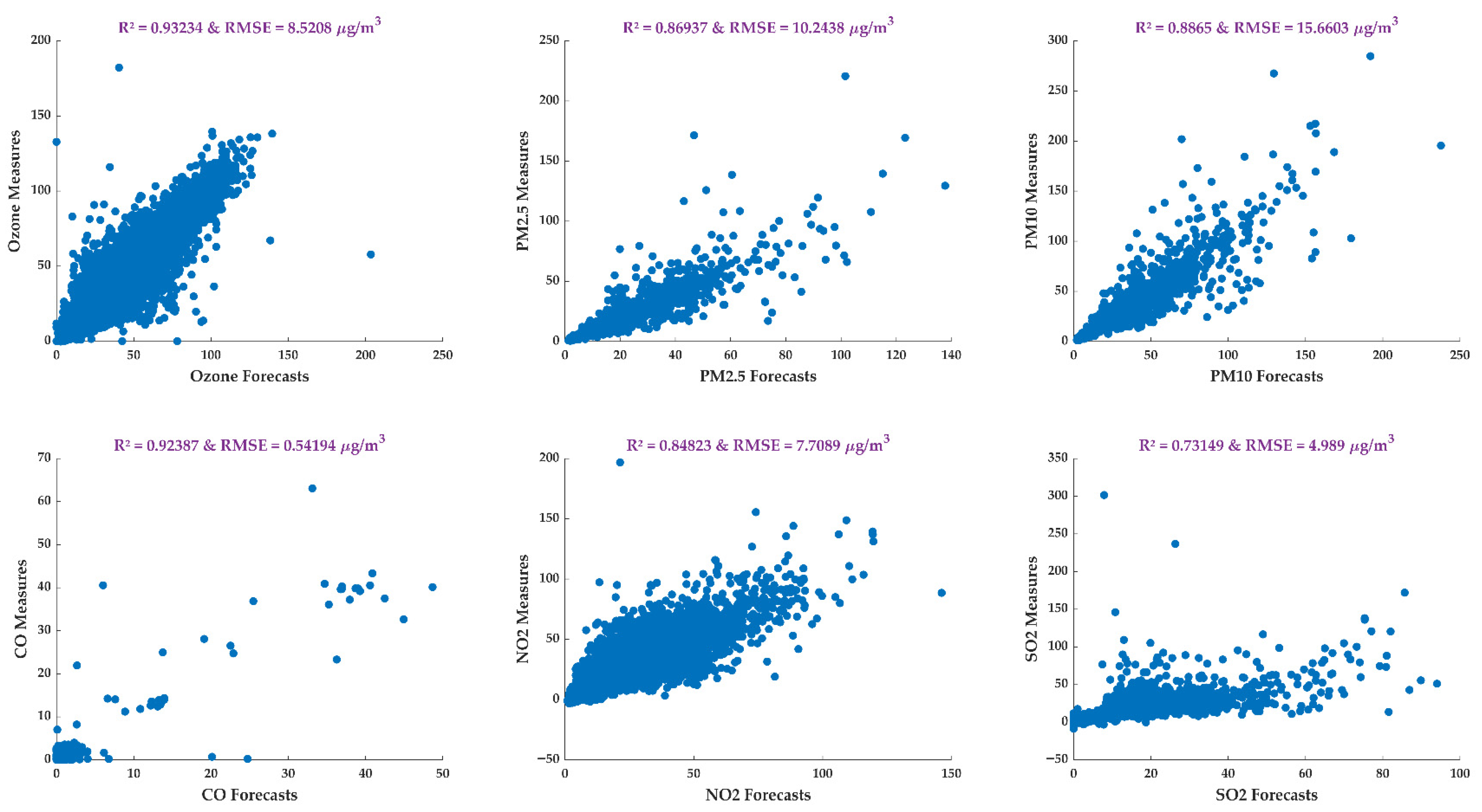
summarises the best-performing Deep-NARMAX models for forecasting the concentrations of the six pollutants included in this study, along with the statistical analysis and the model formulas, highlighting the most commonly employed features. Figure 13 illustrates the corresponding scatter plots. Each subplot compares the observed and predicted values and reports the corresponding R² and RMSE metrics.

For ozone, the Deep-NARMAX model achieves the highest predictive accuracy among all pollutants, with an R² of 0.93. The figure shows a tight alignment between observed and forecast values, especially in the moderate concentration range, indicating that the model effectively learns the photochemical processes driving ozone formation. Deviations are most pronounced at high concentrations, where nonlinear atmospheric chemistry and meteorological interactions become more complex. Even so, forecast performance remains excellent.

The models for PM_2.5 and PM₁₀ also show strong predictive capability, achieving R² values of 0.87 and 0.89, respectively. Both scatter plots show a clear linear trend, though a wider spread is observed at higher concentrations. PM₁₀ shows slightly greater dispersion than PM_2.5, which can be attributed to coarse particles generated by dust events and mechanical processes, which are more challenging to model deterministically. Nevertheless, the results confirm that Deep-NARMAX can reliably reproduce temporal fluctuations in particulate pollutants.

For CO, the model achieves R² = 0.92, with a compact cluster of points near the identity line. The model demonstrates high accuracy in capturing both baseline and peak concentrations. In contrast, the results for NO₂ show a moderate increase in dispersion, particularly at concentrations above 100 µg/m³. With R² = 0.85, the Deep-NARMAX model still performs well, but the increased scatter reflects the complexity of the coupled NO–NO₂–O₃ chemical system. Rapid titration effects and dependence on solar radiation introduce significant variability, challenging short-term forecasting models.

Among the six pollutants, SO₂ is the most difficult, yielding the lowest performance (R² = 0.73). The scatter plot displays higher vertical dispersion, indicating both underestimation and overestimation across a broad concentration range. This reduced accuracy is consistent with the episodic nature of SO₂ emissions, typically driven by industrial combustion sources and abrupt short-lived events, which are harder for data-driven models to learn from limited historical patterns. Despite this, the model still reasonably well captures the general temporal behaviour of SO₂.

4. Conclusions

This study presents a comprehensive, fully integrated AI-driven framework for understanding, predicting, and forecasting the complex dynamics of air pollution from multivariate environmental and atmospheric data. By combining correlation analysis, Granger causality, feature selection, model interpretability, and deep nonlinear forecasting models, the framework ensures both statistical robustness and physical transparency in interpreting pollutant behaviour.

The results highlight the effectiveness of advanced machine learning and deep learning techniques in capturing the nonlinear interactions between pollutants and meteorological variables. Ensemble learning models such as XGBoost and Random Forest, as well as deep neural architectures such as CNNs, consistently outperformed traditional methods on prediction tasks. Feature selection experiments—spanning fifty techniques—showed that metaheuristic and swarm-intelligence-based optimisers provide the most accurate and stable predictor subsets. These methods yielded higher and more reliable R² scores for O₃, PM_2.5, PM₁₀, NO₂, and CO, whereas SO₂ proved the most challenging to model due to its episodic and source-dependent nature.

SHAP-based interpretability analysis confirmed the dominant role of meteorological conditions, especially relative humidity, temperature, wind patterns, and solar radiation, in shaping pollutant concentrations. The NO₂–NO–O₃ photochemical triad also emerged as a central driver of ozone dynamics, while SO₂ and PM₁₀ were frequently identified as the main contributors to deteriorating air quality. These insights bridge the gap between data-driven modelling and atmospheric science by linking model behaviour to known chemical and physical processes.

Forecasting experiments using the Deep-NARMAX framework demonstrated a strong alignment between predicted and observed concentrations, with R² values ranging from 0.73 to 0.93 and low dispersion indicators across pollutants. Ozone, PM_2.5, PM₁₀, and NO₂ showed particularly robust forecast performance, confirming the suitability of nonlinear dynamic models for short-term air quality forecasting. Although the forecasting accuracy for CO and SO₂ was comparatively lower, the results remain satisfactory given the inherent irregularity and noise in these pollutants.

The Air Quality Index (AQI) assessment provided additional insights into temporal patterns of air quality under WHO and EPA guidelines. While current AQI standards rely solely on the maximum pollutant sub-index, our findings suggest that pollutant-specific AQI assessments offer a more informative and nuanced understanding of exposure risks. This approach highlights the importance of revisiting multi-pollutant AQI formulations in future research.

In summary, the proposed hybrid AI framework shows high predictive accuracy, interpretability, and generalisability, providing a powerful tool for real-time air quality prediction and forecasting, as well as for evidence-based environmental policy planning. Future work will focus on expanding the framework to spatiotemporal modelling using real-time sensor networks, incorporating uncertainty quantification, and developing improved multi-pollutant AQI metrics that more accurately reflect actual health risks.