Hourly Regional Rainfall–Runoff Prediction Using Transformer with Water Conservation Constraints

Abstract

This paper introduces MC-former, a Transformer-based rainfall-runoff model designed for hourly regional runoff prediction. Unlike the original Transformer, MC-former integrates a water-balance-guided constraint into the attention layer and enforces physical consistency through a penalty structure. Additionally, MC-former transforms the aggregated input embeddings into the frequency domain via a Fourier transform, enabling more effective modeling of long-range dependencies in hourly runoff data. We tested MC-former on two tasks: regional rainfall-runoff simulation and runoff prediction for ungauged basins with similar hydrogeological units. In the first task, MC-former outperformed baseline models in prediction accuracy. In the second, it improved performance under ungauged conditions, with a notable increase in the Nash–Sutcliffe efficiency coefficient (NSE) in the HUC03 region, surpassing the baseline by nearly 0.08. Furthermore, adopting a strategy of training MC-former with hydrological data from climatically and geologically similar regions further enhanced its predictive accuracy, as demonstrated by consistently higher NSE and Pearson-r values. The MC-former model can support sustainable water resources management and enable transferable prediction of rainfall runoff in ungauged basins.

1. Introduction

Rainfall-runoff prediction has always been one of the core topics in hydrology [1]. Against the backdrop of global climate change leading to increased frequency and intensity of extreme precipitation events, hourly-level rainfall–runoff prediction is particularly crucial for supporting rapid decision-making and effective disaster prevention [2]. Hourly-level prediction can capture the instantaneous dynamics of rainfall peaks and runoff responses, which is essential for real-time response measures including urban flood control, flash flood warning, reservoir operation, and population evacuation. The rainfall–runoff process is influenced by multiple factors including meteorological conditions, watershed topography, and soil characteristics, exhibiting high nonlinearity and spatiotemporal variability [3]. These characteristics pose challenges for traditional conceptual and process-based hydrological models, particularly for hourly-scale prediction. In practice, achieving satisfactory performance often requires nontrivial parameterization and extensive calibration, and the computational burden can become substantial when repeated model evaluations are needed for calibration and sensitivity/uncertainty analyses in large-sample settings. Moreover, model structural simplifications and parameter uncertainty may limit performance for fast hydrological responses at sub-daily scales, motivating data-driven alternatives [4].

To overcome the limitations of traditional models, data-driven methods have gradually become a research hotspot in rainfall–runoff prediction [5,6]. Compared with traditional methods, data-driven approaches can provide higher prediction accuracy and generalization ability by mining complex spatiotemporal patterns in historical data. With the accumulation of high-resolution meteorological and watershed data, machine learning technologies, especially deep learning methods, have made significant progress in rainfall–runoff prediction [7], offering new possibilities for hourly-level prediction.

Although deep learning continuously improves prediction accuracy through optimizing model architectures, its black-box nature remains a significant challenge in the field of disaster prevention. Low interpretability models may undermine decision-makers’ trust, thereby affecting the quality and efficiency of disaster prevention decisions [8]. Therefore, enhancing model interpretability while ensuring prediction accuracy has become a research frontier in the hydrology field [9,10]. Researchers typically address this issue through two approaches: introducing physical constraints and incorporating relevant variables into model calculations. In terms of introducing physical constraints, ref. [11] modified the LSTM architecture using left stochastic matrices to redistribute water among memory units, ensuring water conservation and thus performing excellently in high-flow prediction. Ref. [12] combined reservoir physical mechanism encoding with differentiable modeling strategies to integrate prior physical knowledge into deep learning models, achieving accurate prediction of reservoir operations. Some studies incorporate physical constraints into the loss function of neural networks to implement interpretable physical information in graph neural network flood forecasting models [13]. By adding relevant variables, researchers introduce guiding processes into models based on hydrological physical mechanisms. For example, ref. [14] proposed an entity-aware long short-term memory network for regional hydrological simulation, which significantly outperformed traditional models by directly learning similarities between meteorological data and static watershed attributes, and surpassed region-specific and watershed-specific calibration models in both performance and interpretability. Furthermore, ref. [15,16] significantly improved the simulation accuracy of rainfall-induced flood inundation processes by incorporating topographic data. For catchment-scale rainfall–runoff sequence modeling, topographic information is typically provided as static watershed attributes rather than being explicitly modeled.

In the field of deep learning, Transformer architecture has demonstrated excellent performance in natural language processing, computer vision, and other domains due to its powerful self-attention mechanism [17,18]. Its unique design enables efficient processing of complex patterns in sequential data, making it particularly suitable for high-dimensional spatiotemporal data in rainfall-runoff prediction. Refs. [19,20] pointed out that Transformer-based prediction models are more capable of handling long-term sequence prediction tasks compared to LSTM, as their self-attention mechanism can effectively capture long-distance dependencies. However, some research has indicated [21] that the basic Transformer shows insufficient recognition of long-term memory effects in the time dimension on benchmark datasets such as the CAMELS runoff dataset, requiring further improvements to adapt to the complex dynamics of hydrological systems. The Transformer-based model proposed by [22] significantly outperformed LSTM-based sequence-to-sequence models in 7-day-ahead runoff prediction and demonstrated that its parallel computing capability is more suitable for processing large-scale datasets. Subsequently, a pyramid Transformer rainfall–runoff model was proposed [23], which achieves accurate modeling of regional rainfall runoff by integrating information from different temporal resolutions. Compared to daily runoff prediction tasks, hourly-level prediction involves 24 times more data volume, with more drastic numerical changes, significantly increasing the demand for efficient computation and long-term sequence modeling capabilities [24], while also requiring the model to be more robust. Currently, research on using water balance constraints for deep learning models has mostly focused on daily-scale data, and there are no existing improvements with physical constraints for Transformer-based models.

Reliable hourly rainfall–runoff prediction is essential for sustainable water resources management, including flood early warning, resilient infrastructure operation, drought preparedness, and ecological flow protection. In many regions, decision-making is constrained by limited monitoring capacity and the prevalence of ungauged or poorly gauged basins, which introduces substantial uncertainty in risk assessment and water allocation. Improving predictive skill while maintaining physically plausible behavior therefore contributes to sustainability goals by supporting timely and robust hydrological decision-making under data scarcity and hydro-climatic variability.

Based on the above challenges and opportunities, this study adopts an hourly-level dataset from hundreds of watersheds in the United States and proposes a novel Transformer regional rainfall–runoff model. The model enhances the accuracy and reliability of hourly-level regional rainfall–runoff prediction by incorporating water balance constraints. Additionally, we evaluate the model’s performance across different types of catchment areas.

The contributions of this research are mainly reflected in two aspects. First, we propose a Transformer model for regional runoff prediction that transforms time-domain data into frequency domain for computation and controls the model output to maintain physical rationality through a water balance encoder. Second, we apply the model to an hourly Rainfall–Runoff dataset, demonstrating its advantages compared to baseline models. The paper is structured as follows: Section 2 provides a detailed introduction to the proposed method and model design; Section 3 explains the experimental design and datasets; Section 4 presents experimental results and analysis; Section 5 summarizes the research contributions and outlines future directions.

2. Methods

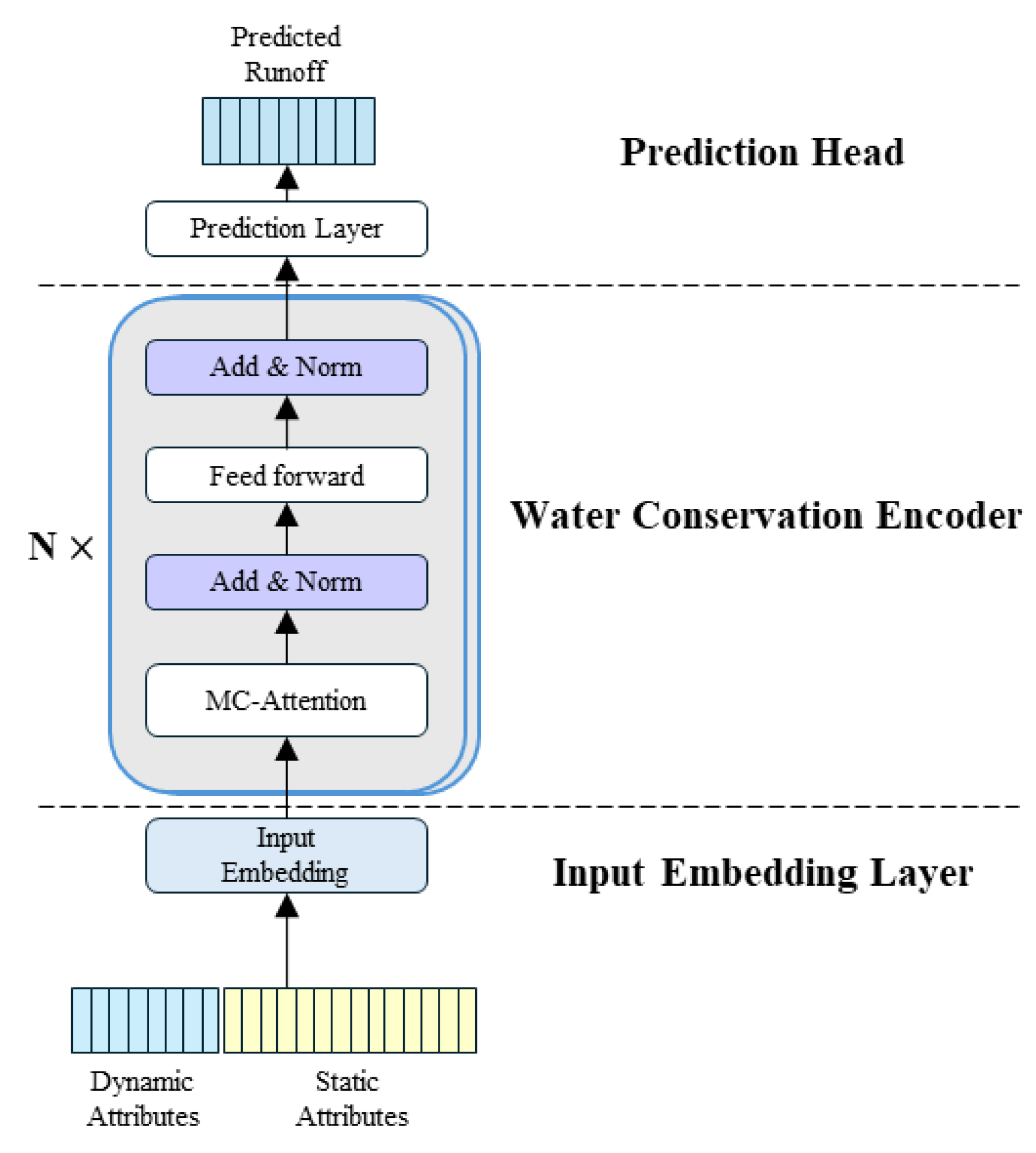
We propose a Transformer-based regional rainfall–runoff model, named MC-former, whose architecture consists of an input embedding layer, a physics-constrained Transformer encoder, and a regression prediction head, as illustrated in Figure 1. The functions of each component are introduced in the following subsections.

2.1. Input Embedding Layer

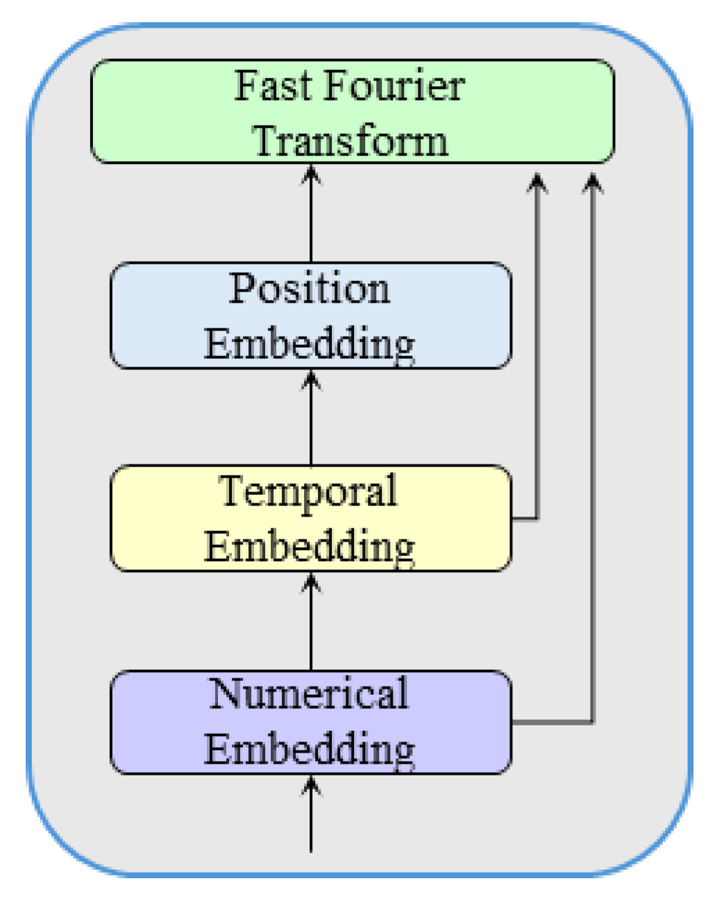
The input embedding layer generates a comprehensive embedding representation for time series data, combining original numerical features, temporal features, and positional information. The input embedding layer structure is shown in Figure 2. When using Transformer architecture models for regional rainfall–runoff modeling, watershed static attributes can effectively distinguish different target watersheds [25], reducing the possibility of catastrophic forgetting in the model. In this context, ref. [14] pointed out that directly concatenating watershed static attributes with dynamic meteorological data is more efficient than independently computing watershed static attributes. Therefore, watershed static attributes are concatenated with dynamic meteorological variables to form the input sequence of the model. Different types of input features are normalized separately using min–max scaling to eliminate scale differences and improve training stability.

First, the input sequence undergoes linear transformation, mapping each input feature to a high-dimensional space to obtain numerical embeddings. After that, temporal information is mapped to the embedding space. Most time series forecasting models based on Transformer architecture require hierarchical global timestamp information to encode seasonal and long-term ordinal information [26,27] to obtain temporal embeddings. Finally, positional embeddings are used to generate a position vector for each time step’s input position. We adopt the most commonly used sine and cosine functions in Transformer-like models for positional embedding, with the specific formula as follows:

$$PE\left(i,2k\right)=\sin \left({\displaystyle \frac{i}{{\mathrm{10,000}}^{\frac{2k}{d_{model}}}}}\right)$$

(1)

$$PE\left(i,2k+1\right)=\cos \left({\displaystyle \frac{i}{{\mathrm{10,000}}^{\frac{2k}{d_{model}}}}}\right)$$

(2)

The three embeddings are added to combine numerical, temporal, and positional features. Zhou [28] pointed out that frequency domain representation can effectively capture and model frequency features in time series, thereby improving model performance, especially when processing time series data with obvious periodicity or frequency patterns. Since rainfall–runoff data typically exhibits significant seasonal or periodic variations, we apply fast Fourier transform to the combined input embedding (which integrates numerical, temporal, and positional information), converting the time domain data into frequency domain data for computation in the encoder layer, and enriching long-range temporal dependencies, as expressed in Equation (3):

$$E= E_{num}+E_{temp}+E_{pos} , F={\mathcal{F}}_t\left(E\right)$$

(3)

where ${\mathcal{F}}_t(·)$ denotes the 1D FFT applied along the time dimension, and the encoder then takes $F$ as its input. Here, the Fourier transform is employed as a representation-level transformation to expose periodic and long-range temporal patterns to the attention mechanism, rather than as a strict physical spectral analysis of the hydrological signal.

2.2. Physics-Constrained Transformer Encoder

The model we propose is based on the Transformer model, whose encoder consists of multiple encoder layers, each composed of an attention layer and a feed-forward network layer. The core component of the attention layer is the attention mechanism. The attention mechanism calculates the similarity between query vectors (Query) and key vectors (Key) and uses this as weights to perform a weighted sum of value vectors (Value), thereby enabling the model to dynamically aggregate different positions in the input sequence. The process can be described as follows:

$$Attention\left(Q,K,V\right)=f\left(Similarity\left(Q,K\right)·V\right)$$

(4)

where $Q$ is the query vector, $K$ is the key vector, $V$ is the value vector, and the function f transforms the result into an output. This output can then be used for further computations in the neural network.

Depending on the method of calculating similarity, there are also many variants of the attention mechanism, among which the original Transformer adopts the most common scaled dot-product attention. The correlation between each query vector and key vector is described by the attention weight matrix, and the attention weight calculation formula is as follows:

$$W_{attn}=softmax\left({\displaystyle \frac{Q{K}^T}{\sqrt{d_k}}}\right)$$

(5)

where $d_k$ is the dimension of the key.

The output of the scaled dot-product attention can be simplified as follows:

$$Attention=W_{attn}·V$$

(6)

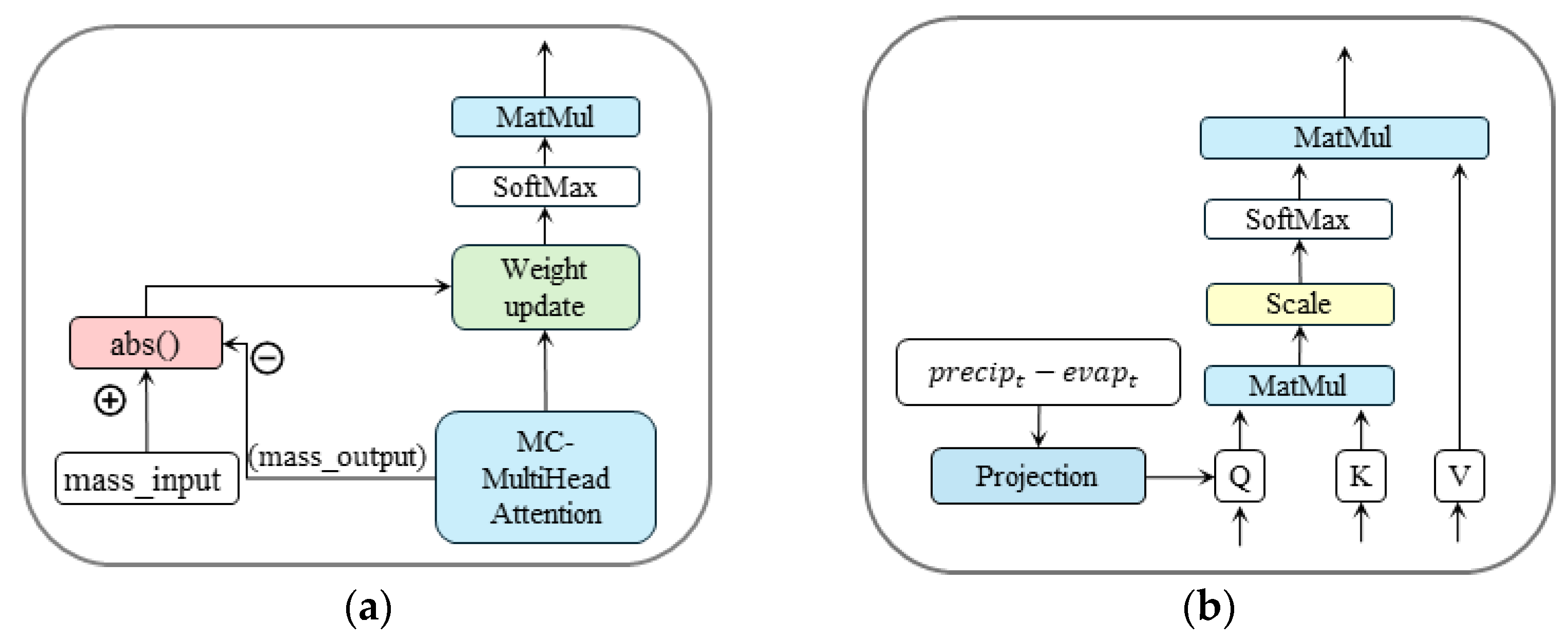
We define MC-attention (mass conserving attention) as a modified self-attention mechanism in which cumulative water input and a layer-wise mass-tracking state are explicitly tracked, and their discrepancy is used to bias attention weights toward physically consistent aggregation.

Compared with standard scaled dot-product attention, MC-attention introduces two key modifications: (1) re-engineering the forward propagation of the multi-head attention module to maintain the layer-wise mass-tracking state, and (2) integrating cumulative water-input signals into the attention computation. The overall structure is illustrated in Figure 3.

Following a simplified conceptual view of the surface water balance, precipitation and evapotranspiration are used to construct a cumulative input water signal that serves as a guiding constraint rather than an explicit discharge equation. Specifically, the cumulative input water volume from the beginning of the input sequence to time step i is defined as follows:

$$mas{s}_{input}\left(i\right)=\sum _{t\le i}\left(preci{p}_t-eva{p}_t\right)$$

(7)

where $preci{p}_t$ denotes the rainfall amount at time $t$, and $eva{p}_t$ denotes the potential evapotranspiration at time $t$. This cumulative net-input term is used as a guiding constraint signal rather than an explicit runoff generation equation. Storage-related processes such as initial basin storage, groundwater delay, and subsurface routing are not explicitly represented in Equation (6). This does not imply zero initial storage; rather, storage dynamics are not explicitly parameterized here and are expected to be learned implicitly from long input sequences and catchment attributes.

We enhance the calculation method of query vectors in the attention layer by projecting the input quality term onto each query, allowing the model to learn and preserve the patterns of water quantity transformation. Meanwhile, to continuously track the amount of water discharged by the model during the self-attention calculation at each layer, we maintain a cumulative water amount from the previous layer output ${mass}_{output}^{(l-1)}$ for each query position.

If the encoder has a total of k layers, $l\in \left\{1,\dots ,k\right\},$ we set ${mass}_{output}^{\left(0\right)}\equiv 0$. Following the practice in MC-LSTM, we designate the 0th output channel of each encoder layer as discharge. This choice is empirically justified through a sensitivity analysis (Appendix A.1), which shows that the model is not overly sensitive to channel selection, while channel 0 provides the most stable and robust performance across basins. Then, the accumulated water volume from the previous layer output at the $i$-th time step can be described as follows:

$${mass}_{output}^{\left(l-1\right)}\left(i\right)=\sum _{k=1}^{l-1}{h}_{i,0}^{\left(k\right)}=\sum _{k=1}^{l-1}{discharge}_i^{\left(k\right)}$$

(8)

where $h_{i,0}^{\left(k\right)}$ denotes the 0th output channel of the $k$-th encoder layer at time step $i$. This quantity represents a layer-wise mass-tracking state rather than a physical time integration; it is used to monitor the cumulative discharge generated across encoder layers.

For Transformer architecture, due to the lack of recurrent structures, relying solely on water quantity input to guide attention to achieve water conservation is not realistic. We need to guide the attention layer output toward consistent water-conservation behavior. Therefore, it is necessary to calculate the difference between the input water quantity and the output water quantity of each encoder layer to obtain the water quantity difference penalty term to bias the attention computation in the $l$-th layer:

$$W_{penalty}^{\left(l\right)\left(i\right)}=\left|mas{s}_{input}\left(i\right)-{mass}_{output}^{\left(l-1\right)}\left(i\right)\right|$$

(9)

where $mas{s}_{input}$ is the input cumulative water amount, and ${mass}_{output}^{\left(l-1\right)}$ is the output cumulative water amount from the previous layer. In implementation, $W_{penalty}^{\left(l\right)\left(i\right)}$ is computed for each query time step i and then broadcast along the key dimension to form a penalty matrix compatible with the L × L attention-weight matrix. For each encoder layer, the cumulative output water mass is tracked in a layer-wise manner. Before computing attention in the $l$-th layer, the model uses the mass-tracking state ${mass}_{output}^{\left(l-1\right)}$ accumulated up to the immediately preceding layer $\left(l − 1\right)$ at each time step $i$. After the attention output of layer $l$ is obtained, this mass-tracking state is updated and passed to the next layer, enabling progressive enforcement of mass conservation across the depth of the network. The resulting water-mass discrepancy is incorporated into the attention weight computation of the current layer, guiding the attention mechanism toward physically consistent runoff generation.

After obtaining the water-mass difference penalty term, we can adjust the weights of the water conservation attention in each encoder layer by taking the logarithm of the standard attention weight matrix W and subtracting the penalty term:

$${\tilde{L}}^{\left(l\right)}=\log \left(W_{attn}^{\left(l\right)}+\epsilon \right)-\lambda ·W_{penalty}^{\left(l\right)}$$

(10)

where $\lambda$ is the coefficient regulating the conservation strength, and $\epsilon$ is a small value to prevent the log calculation from becoming zero. Here, $W_{attn}^{\left(l\right)}$ ∈ ${\mathrm{R}}^{\mathrm{L}\times \mathrm{L}}$ is the row-wise softmax-normalized attention-weight matrix.

When $\lambda > 0$, it makes the attention bias toward the group of keys that are better for water conservation. Afterwards, we renormalize ${\tilde{L}}^{\left(l\right)}$ by applying a row-wise softmax over the key dimension, and use the resulting normalized weights to combine V, obtaining the conservation-guided attention output:

$$Attentio{n}_{output}=softmax\left({\tilde{L}}^{\left(l\right)}\right)·V$$

(11)

After the attention layer output undergoes residual connection and layer normalization, it enters the feed-forward network layer. After performing linear transformation and nonlinear activation function calculations on the input, residual connection and layer normalization operations are performed again, and the output result is sent to the prediction head.

2.3. Prediction Head

In time series forecasting tasks, encoder-only architectures demonstrate excellent performance in many scenarios, especially when efficiently processing long sequence data [29]. First, we use inverse Fourier transform to convert the runoff frequency domain predictions from the encoder output into time domain predictions. Then, we use a linear layer as the prediction head to generate the time-domain-predicted runoff sequence. It should be noted that the inverse Fourier transform in MC-former is not intended to reconstruct a physically interpretable time-domain signal from a strictly linear spectral representation. The inverse FFT is used as a representation-level mapping to project learned frequency-aware features back to the time domain for prediction, rather than as a strict inverse spectral operator. Multi-step forecasts are generated autoregressively (rolling), i.e., the model produces one-step-ahead predictions iteratively until the full forecast horizon is obtained.

2.4. Metrics and Benchmark

For performance evaluation, we adopt the following metrics: Nash–Sutcliffe efficiency (NSE), Pearson correlation coefficient (r), Kling–Gupta efficiency (KGE), and mean squared error (MSE).

NSE is a metric that measures the degree of agreement between the hydrological model’s predictions and observed data. Its value ranges from negative infinity to 1, with a value closer to 1 indicating better model fit. The formula for calculating NSE is as follows:

$$\mathrm{N}\mathrm{S}\mathrm{E}=1-{\displaystyle \frac{{\sum }_{i=1}^n{\left(Q_{sim,i}-Q_{obs,i}\right)}^2}{{\sum }_{i=1}^n{\left(Q_{sim,i}-\overline{Q_{obs}}\right)}^2}}$$

(12)

where $Q_{obs,i}$ is the observed runoff at time step $i$, $Q_{sim,i}$ is the predicted runoff at time step $i$, $n$ is the number of time steps, and $\overline{Q_{obs}}$ is the mean of the observed runoff.

The Pearson correlation coefficient is commonly used to evaluate the linear relationship and correlation between hydrological model predictions and measured data. The closer the value is to 1, the stronger the linear relationship between the model predictions and measured values, indicating good model performance. The calculation formula for the Pearson correlation coefficient is as follows:

$$\mathrm{r}={\displaystyle \frac{cov\left(Q_{sim},Q_{obs}\right)}{\sigma \left(Q_{sim}\right)·\sigma \left(Q_{obs}\right)}}$$

(13)

where $cov\left(Q_{sim},Q_{obs}\right)$ is the covariance between simulated and observed data; $\sigma \left(Q_{sim}\right)$, $\sigma \left(Q_{obs}\right)$ are the standard deviations of simulated and observed data.

KGE comprehensively evaluates model performance by integrating multiple metrics. Its value ranges between negative infinity and 1, with the KGE value closer to 1 indicating a better fit of the model to the data. The calculation formula for KGE is as follows:

$$\mathrm{K}\mathrm{G}\mathrm{E}=1-\sqrt{{\left(\mathrm{r}-1\right)}^2+{\left({\displaystyle \frac{\sigma \left(Q_{sim}\right)}{\sigma \left(Q_{obs}\right)}}-1\right)}^2+{\left({\displaystyle \frac{\overline{Q_{sim}}}{\overline{Q_{obs}}}}-1\right)}^2}$$

(14)

MSE is a commonly used loss function in regression tasks, used to measure the mean squared error between model predictions and actual values. Its formula is as follows:

$$\mathrm{M}\mathrm{S}\mathrm{E}={\displaystyle \frac{1}{n}}\sum _{i=1}^n{\left(Q_{sim,i}-Q_{obs,i}\right)}^2$$

(15)

In addition to NSE, KGE, Pearson correlation, and MSE, three flow regime-specific metrics are used to further diagnose model performance under different runoff conditions: high flow bias (FHV), medium flow bias (FMS), and low flow bias (FLV). These metrics quantify relative bias under high-, medium-, and low-flow conditions, respectively, and complement NSE and KGE by explicitly assessing flood peaks, normal flow stability, and low-flow behavior. These metrics are defined mathematically as follows:

$$\mathrm{F}\mathrm{H}\mathrm{V}= {\displaystyle \frac{{\sum }_{i\in {\mathsf{{\rm T}}}_H}\left(Q_{sim,i}-Q_{obs,i}\right)}{{\sum }_{i\in {\mathsf{{\rm T}}}_H}{Q}_{obs,i}}}\times 100$$

(16)

$$\mathrm{F}\mathrm{L}\mathrm{V}={\displaystyle \frac{{\sum }_{i\in {\mathsf{{\rm T}}}_L}\left(Q_{sim,i}-Q_{obs,i}\right)}{{\sum }_{i\in {\mathsf{{\rm T}}}_L}{Q}_{obs,i}}}\times 100$$

(17)

$$\mathrm{F}\mathrm{M}\mathrm{S}={\displaystyle \frac{{\sum }_{i\in {\mathsf{{\rm T}}}_M}\left(Q_{sim,i}-Q_{obs,i}\right)}{{\sum }_{i\in {\mathsf{{\rm T}}}_M}{Q}_{obs,i}}}\times 100$$

(18)

${\mathsf{{\rm T}}}_H{,\mathsf{{\rm T}}}_M,{\mathsf{{\rm T}}}_L$ are defined based on quantiles of the observed discharge $Q_{obs}$. Specifically, ${\mathsf{{\rm T}}}_H$ denotes the set of time indices corresponding to high-flow conditions, defined as the top 2% of observed flows. ${\mathsf{{\rm T}}}_M$ represents medium-flow conditions, defined as observations between the 20% and 70%. ${\mathsf{{\rm T}}}_L$ corresponds to low-flow conditions, defined as the bottom 30% of observed flows. These percentile-based definitions ensure that the flow regimes are determined in a basin-specific and scale-invariant manner.

We will use the Transformer model [25] and the LSTM model [24] as baseline models to compare with our proposed model. All baseline models were reimplemented/retrained under the same experimental setup and data splits as MC-former (training/validation/test), rather than using published performance values. Both baseline models also use static watershed variables for computation; in other words, the baseline models also have regional runoff prediction capabilities. The hyperparameter values for the baseline models follow the specifications in their respective papers, while other training settings (e.g., input window, optimizer, and early-stopping criterion) are kept consistent across models whenever applicable to ensure a fair comparison.

3. Data and Experimental Setup

3.1. Dataset

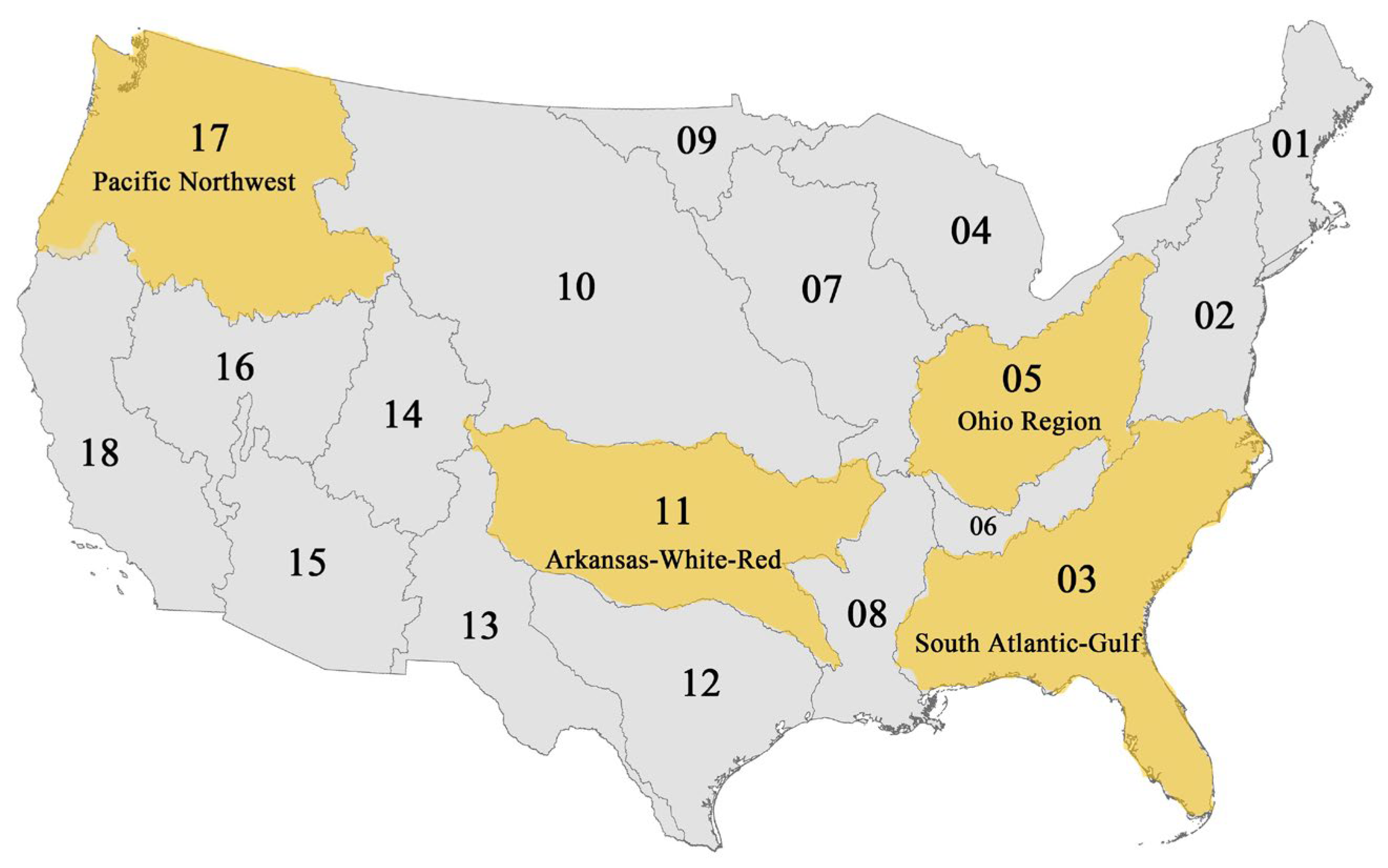
Our task is to achieve regional rainfall-runoff prediction at an hourly scale using the model; therefore, we need static watershed attributes and hourly-level dynamic data. We selected the same 27 static watershed attributes from the CAMELS dataset [30] to participate in the model calculation, as shown in

Table 1. Meteorological forcings and catchment attributes.

Meteorological forcings

Total precipitation

Potential evaporation

Shortwave radiation

Specific humidity

Temperature

Static catchment attributes

Precipitation-Mean

PET-Mean: mean daily potential evapotranspiration

Aridity-Index: ratio of PET mean to Precipitation mean

Precip-Seasonality: estimated by representing annual precipitation and temperature as sin waves, where positive (negative) values indicate precipitation peaks during the summer (winter)

Snow-Fraction: fraction of daily precipitation with temperatures below 0

High-Precip-Frequency: frequency of high-precipitation days (≥5 times mean daily precipitation)

High-Precip-During: average duration of high-precipitation events (number of consecutive days with ≥5 times mean daily precipitation)

Low-Precip-Frequency: frequency of dry days (less than 1 mm/day)

Low-Precip-During: Average duration of dry periods (number of consecutive days with precipitation less than 1 mm/day)

Catchment-Mean-Elevation

Catchment-Mean-Slope

Catchment-Area

Forest-Fraction: fraction of catchment covered by forest

LAI-Max: maximum monthly mean of leaf area index

LAI-Difference: difference between the max. and min. mean of the leaf area index

GVF-Max: maximum monthly mean of green vegetation fraction

GVF-Difference: difference between the maximum and minimum monthly mean of the green vegetation fraction

Soil-Depth-Pelletier: depth to bedrock (maximum 50 m)

Soil-Depth-STATSGO: soil depth (maximum 1.5 m)

Soil-Porosity: volumetric porosity

Soil-Conductivity: saturated hydraulic conductivity

Max-Water-Content: maximum water content of the soil

Sand-Fraction

Silt-Fraction

Clay-Fraction

Carbonate-Rocks-Fraction: fraction of the catchment area characterized as carbonate sedimentary rocks

Geological-Permeability: surface permeability (log10)

. The CAMELS dataset includes data from 671 catchments in the United States, which can be divided into 18 hydrologic units based on the hydrologic unit code map provided by the United States Geological Survey. As shown in Figure 4, these hydrologic units correspond to geographical regions that represent the watershed of a major river or the combined watershed of multiple rivers. Additionally, we adopted the USGS hourly runoff values used by [24] and the NLDAS-2 hourly meteorological data product [31] recorded since 1979, and we used consistent processing methods. The meteorological forcing inputs are shown in Table 1. From the original 671 CAMELS basins, a total of 471 basins were retained for this study. Basin selection was based solely on data availability and temporal consistency at the hourly scale. Specifically, basins with missing periods in hourly USGS streamflow records, irregular hourly sampling, or incomplete temporal overlap between USGS streamflow and basin-averaged NLDAS-2 meteorological forcings were excluded. No filtering was performed based on hydro-climatic conditions, basin size, or physiographic attributes.

3.2. Experimental Design

3.2.1. Rainfall-Runoff Prediction in 471 Basins

In this experiment, our objective was to demonstrate the performance of the proposed model and baseline models in regional rainfall–runoff modeling. This paper uses data from 471 valid catchments, and all selected watersheds are within the coverage of the CAMELS dataset. The dataset was divided into a training set (1 October 1980–30 September 1995), a validation set (1 October 1995–30 September 2000), and a test set (1 October 2000–30 September 2005). The training set was used to update learnable parameters through backpropagation, after which the model was applied to the validation set to evaluate its accuracy on unseen data. After determining the optimal hyperparameters, the test set is used to evaluate the model performance. In this work, our objective is regional rainfall–runoff hindcasting given observed meteorological forcings, rather than long-term extrapolation across changing climate regimes. The effects of climate variability are therefore implicitly reflected in the meteorological inputs (e.g., precipitation and temperature). Moreover, the temporally separated training, validation, and test splits provide an implicit evaluation under different climate conditions. Explicit treatment of non-stationarity and regime-aware modeling is beyond the scope of this study and is left for future work.

3.2.2. Rainfall–Runoff Prediction in Different Hydrogeological Units

In this experiment, our objective is to investigate the model’s performance in different hydrogeological units and the impact of hydro-climatic and physiographic similarity of hydrogeological units on ungauged streamflow prediction performance. Based on the hydrogeological unit system established by the United States Geological Survey, and considering flow diversity and experimental representativeness, we selected four hydrogeological units for the experiment, as shown in

Table 2. Hydrogeological Unit Information.

Hydrogeological Unit Code	Climate and Topography
HUC03	Humid subtropical climate with hot, humid summers, mild winters, and frequent tropical cyclones. The region features vast coastal plains with dense river networks, wetlands, and gradually rising hills/low mountains. Dominated by sedimentary plains and shallow soils.
HUC05	Humid continental climate with warm, humid summers and cold winters. Precipitation is evenly distributed year-round. Characterized by low to medium mountains, river valleys, and floodplains.
HUC11	Humid subtropical to temperate sub-humid climate with hot, humid summers, mild winters, and frequent thunderstorms. Terrain includes the Ozark Plateau, plains, hills, river valleys, and alluvial plains, transitioning from mountainous to flat areas.
HUC17	Maritime climate along the coast with abundant precipitation; inland areas experience a temperate climate with snowy winters and dry summers. Precipitation mainly occurs in winter. The region is marked by varied terrain including the Cascade and Coast Mountains, cliffs, canyons, and volcanic landforms.

. Ref. [25] to conduct the experiment, in order to verify the model’s performance in ungauged basins. The model training did not involve data from the target watershed during any period; it was trained only on similar watersheds.

3.3. Hyperparameter Settings and Experimental Environment

We employed a hyperparameter grid search to determine the model’s hyperparameters. Due to computational resource limitations, we first selected three sets of hyperparameters in 30 watersheds, then applied them to all watersheds to find the optimal set, as shown in

Table 3. The values of hyperparameters.

Hyperparameters	Value
Batch size	256
Dropout rate	0.1
$\lambda$	0.5
Seq_len	336
Learning rate	0–10: 0.001 11–20: 0.0005 21–30: 0.0001
epoch	30
d_model	512
n_heads	8
n_layers	2

. We conducted a sensitivity analysis of λ (Appendix A.2) and found that λ = 0.5 was within a stable range that balanced accuracy and conservation. All models were implemented based on Python 3.9 using the PyTorch (2.4.1) framework. The libraries we used for data processing included Numpy (1.24.4), Pandas (1.3.3), and Matplotlib (3.7.0). All experiments were conducted on a single NVIDIA GeForce RTX 3080 (24 GB memory).

4. Results and Discussion

We used the relevant metrics described in Section 2.4 to assess model performance, demonstrate the runoff prediction performance of MC-former in various scenarios, and analysed the impact of different training data on the accuracy of prediction in ungauged basins.

4.1. Predict Performance of 471 Basins

This experiment used 18 types of hydrogeological units, totalling 471 watershed data for regional rainfall–runoff modelling, and the results of each model’s performance metrics are shown in

Table 4. 471 Basins Runoff Prediction Performance.

Model	MSE	Median NSE	Mean NSE	Median KGE	Mean KGE	Median Pearson	Mean Pearson
MC-former	0.011	0.593	0.556	0.656	0.615	0.796	0.770
Transformer	0.009	0.546	0.519	0.643	0.613	0.761	0.749
LSTM	0.012	0.562	0.531	0.622	0.596	0.771	0.754

. Overall, although the Transformer baseline shows a slight advantage in MSE, MC-former achieves better performance on the other major metrics (including NSE, KGE, and Pearson correlation). In particular, MC-former yields higher NSE and KGE than both Transformer and LSTM, suggesting improved efficiency and better reproduction of runoff dynamics. Note that a lower MSE does not necessarily imply better hydrological skill; the Transformer tends to produce smoother, mean-biased hydrographs with reduced variance, which can dampen peaks and flow variability. As a result, NSE and KGE, being more sensitive to bias and variance matching, become worse even when the MSE is slightly lower.

Additionally, we present the cumulative distribution function (CDF) plots of NSE for the first 12 h runoff predictions of all models in Figure 5. The MC-former model consistently outperforms the other two benchmark models (Transformer and LSTM) on these two performance metrics. The CDF curve of MC-former is steeper and rapidly approaches 1, indicating that it can provide high-accuracy predictions in most cases. The above results demonstrate the powerful capability of MC-former in regional rainfall–runoff modelling. With regard to attention mechanism and water balance constraints, MC-former is more suitable for large-scale hydrological datasets than traditional Transformer and LSTM models.

4.2. Predict Performance of Specific Hydrogeological Units

4.2.1. Predict Performance of Different Hydrogeological Units

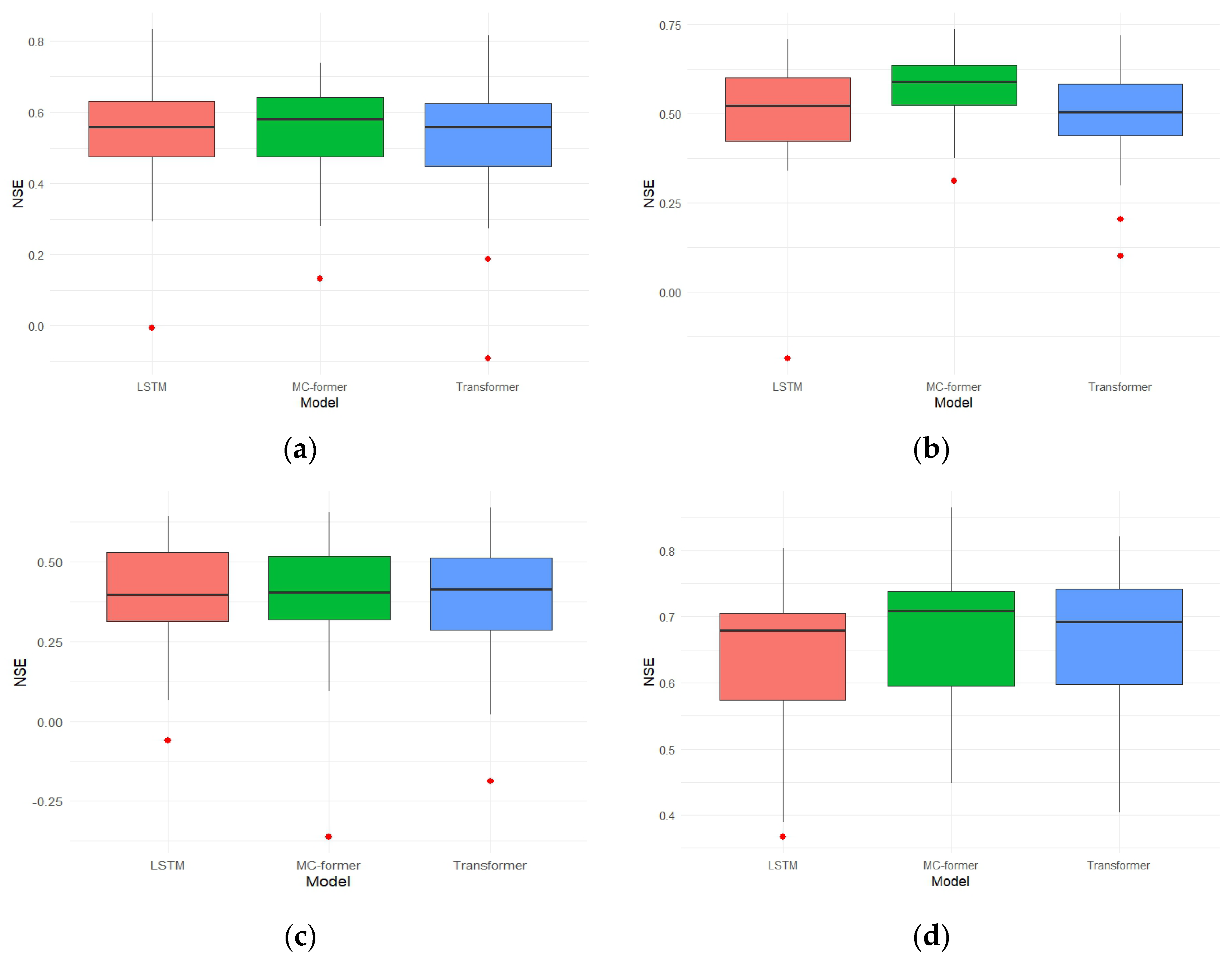
We modelled each hydrogeological unit separately to investigate the model’s runoff prediction performance across different hydrogeological units and compared it with the baseline models. The corresponding boxplots are shown in Figure 6. Our model achieved a higher median NSE than the two baseline models across all four hydrogeological units, with the most significant gap observed in the HUC05 region.

We also analysed other metrics for each model across different hydrogeological units, as shown in

Table 5. KGE and Pearson Value for each Model.

Model	HUC03		HUC05		HUC11		HUC17
	KGE	r	KGE	r	KGE	r	KGE	r
MC-former	0.655	0.790	0.685	0.765	0.534	0.688	0.680	0.851
Transformer	0.601	0.771	0.646	0.742	0.475	0.669	0.671	0.848
LSTM	0.608	0.778	0.659	0.752	0.459	0.688	0.629	0.824

. Overall, MC-former demonstrates superior performance across most evaluation metrics and hydrogeological units, although improvements may manifest differently across metrics in specific regions. For example, in HUC11, the Pearson correlation of MC-former is comparable to that of LSTM, while improvements are observed in other efficiency- and error-based metrics. These results suggest that imposing a water-conservation constraint helps regulate the model’s behavior toward physically plausible runoff generation and improves overall predictive performance compared to the baseline models.

4.2.2. Predict Performance of Ungauged Basins

As mentioned previously, ungauged performance was one of the metrics for evaluating whether models have truly learned regional hydrological relationships. To improve the statistical reliability of our conclusions, we randomly selected 5–10 ungauged basins within each HUC region for evaluation. The median NSE of each model across the selected ungauged basins is reported in

Table 6. Median NSE value of each model in Ungauged Basins.

Model	HUC03 (n = 5)	HUC05 (n = 7)	HUC11 (n = 10)	HUC17 (n = 10)
MC-former	0.562	0.607	0.588	0.742
Transformer	0.484	0.506	0.511	0.720
LSTM	0.479	0.517	0.506	0.734

. The results indicate that MC-former generally achieved higher NSE values across the evaluated ungauged basins, with more pronounced improvements in the HUC03 region, where baseline models exhibited relatively weaker performance. On average, MC-former improved NSE by approximately 0.08 compared to the baseline models.

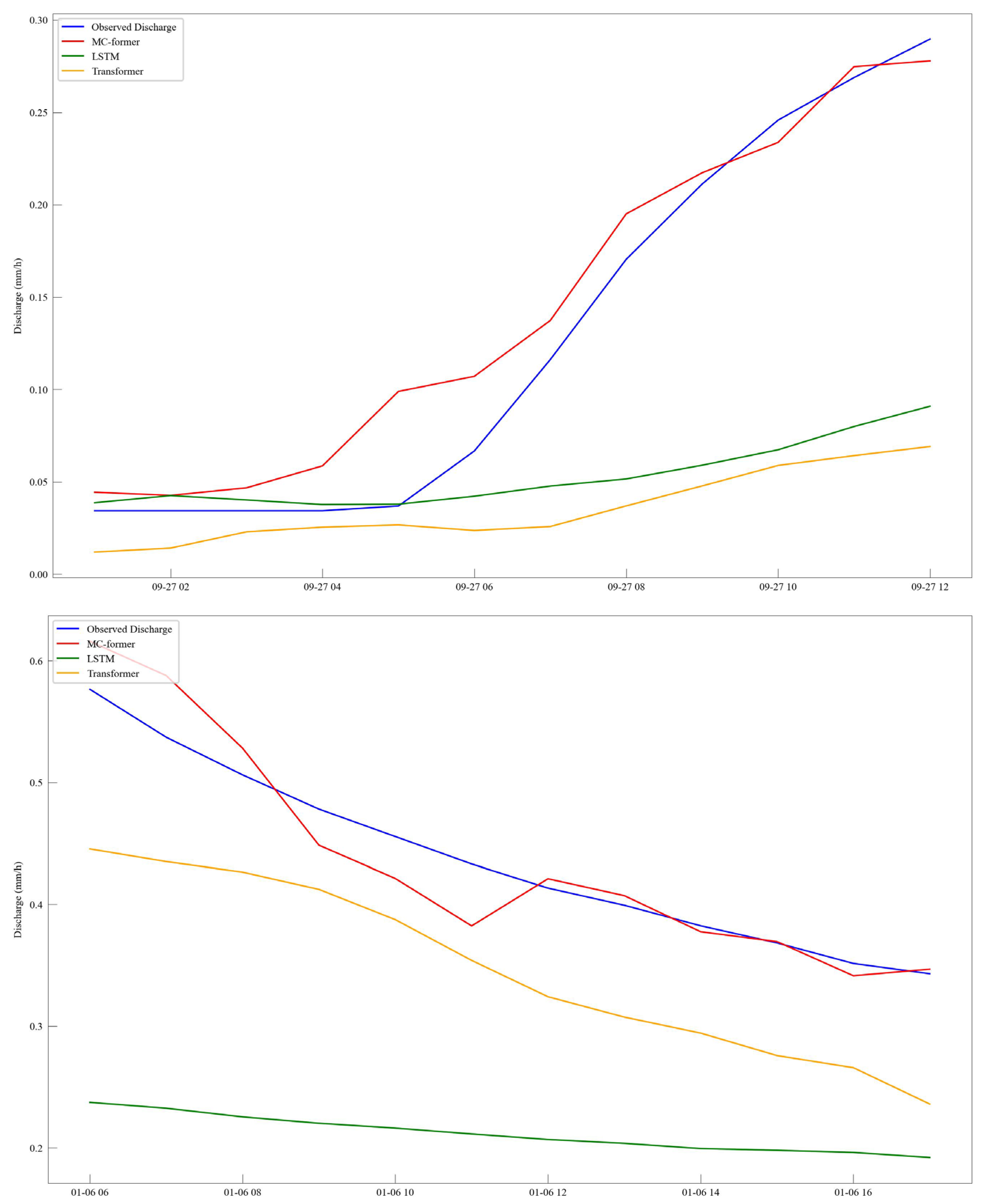
Additionally, we also show the runoff variations of each model during random consecutive 12-h periods in 03144000. As shown in Figure 7, the MC-former curve has smaller fluctuations compared to the baseline models and can well predict peak flows, further demonstrating the excellent generalization of the MC-former model, indicating that it can better learn regional hydrological relationships, thereby improving ungauged runoff prediction performance.

4.2.3. Regional Proximity Effect for Ungauged Basin Forecasting

Hydro-climatic and physiographic similarity is hypothesized to be a key factor enabling effective knowledge transfer in ungauged basin prediction. To evaluate the influence of basin similarity on model performance, we designed two groups of region-combination experiments: (HUC05, HUC06, HUC17) and (HUC04, HUC07, HUC12). The similarity classification follows a Euclidean-distance criterion computed using the hydro-climatic and physiographic variables listed in

Table 7. Climate and Topography in Different HUC Regions.

HUC	p_Mean (mm/day)	q_Mean (mm/day)	Runoff_Ratio	Pet_Mean (mm/day)	Elev_Mean (m)	Slope_Mean (m/km)
HUC05	3.516	1.549	0.435	2.520	526.363	26.491
HUC06	4.501	2.205	0.479	2.859	858.472	72.368
HUC17	5.218	4.083	0.709	2.389	1077.201	111.887
HUC04	2.649	1.081	0.403	2.276	363.053	10.524
HUC07	2.709	0.764	0.281	2.472	264.130	5.773
HUC12	2.553	0.382	0.135	3.635	320.985	10.339

. Specifically, we compute pairwise Euclidean distances in the standardized variable space (to remove scale effects across different attributes). Before distance computation, each variable in Table 7 is standardized by z-score normalization (zero mean and unit variance) across the six HUC regions considered. Euclidean distances are then computed in this standardized space with equal weights assigned to all variables, avoiding subjective tuning of attribute importance. Based on the computed distances, HUC05 is classified as similar to HUC06 and dissimilar to HUC17; likewise, HUC04 is classified as similar to HUC07 and dissimilar to HUC12. This multi-pair design reduces the risk that our conclusions are driven by a single regional comparison and provides a more balanced assessment of similarity-based transfer for ungauged basin prediction.

Therefore, we modeled runoff using two training strategies: one using rainfall–runoff data from similar region (e.g., HUC05 + HUC06) for model training; the other using rainfall–runoff data from dissimilar region (e.g., HUC05 + HUC17) for model training. The results are shown in

Table 8. Ungauged basins Prediction Performance Under Different Strategies.

Strategy	NSE	KGE	Pearson	FHV	FMS	FLV	MSE
Dissimilar (HUC05 + HUC17) (n = 5)	0.566	0.780	0.779	0.236	−15.548	−649.21	0.007
Similar (HUC05 + HUC06) (n = 5)	0.734	0.701	0.864	−21.335	−19.143	−3.03	0.004
Dissimilar (HUC04 + HUC12) (n = 5)	0.498	0.484	0.722	−13.103	−12.081	−652.703	0.007
Similar (HUC04 + HUC07) (n = 5)	0.559	0.495	0.776	−42.088	−12.659	−50.464	0.005

.

Based on the analysis of multiple performance metrics, training with hydro-climatically similar regions consistently leads to better overall prediction accuracy for ungauged basins. In both regional groups, the similarity-based strategies (HUC05 + HUC06 and HUC04 + HUC07) achieve higher NSE and Pearson correlation coefficients, together with lower MSE values, indicating improved overall error control and representation of flow dynamics. In contrast, training with hydro-climatically dissimilar regions shows a clear advantage in peak-flow representation. For both HUC05 and HUC04 groups, the dissimilar-region strategies yield FHV values that are substantially closer to zero than those obtained with similar-region training, suggesting reduced bias in simulating high-flow extremes. These results demonstrate that hydro-climatic similarity primarily governs overall predictive accuracy, while exposure to dissimilar-region data can enhance the model’s ability to capture peak-flow behavior. Consequently, the choice of training strategy should be guided by the specific prediction objectives, balancing general accuracy against improved representation of hydrological extremes.

5. Conclusions

This study developed MC-former, a physics-constrained Transformer framework for hourly regional rainfall–runoff prediction, in which attention aggregation is guided by water-balance-based constraints. Extensive experiments across 471 basins indicate that the proposed physics-guided attention mechanism yields robust performance gains over baseline models, while enhancing physics-guided interpretability in data-driven hydrological modelling.

Beyond overall accuracy gains, the results provide two key insights for regional and ungauged basin prediction. First, training with hydro-climatically and physiographically similar regions substantially improves general predictive skill, indicating that attribute-based similarity offers a principled basis for regional knowledge transfer. Second, incorporating complementary dissimilar-region data can help mitigate bias in peak-flow simulation, suggesting a trade-off between overall accuracy and extreme-event representation.

Despite these advantages, the proposed framework may face limitations under extreme flash-flood conditions and in snow-dominated basins, where additional physical processes are not explicitly represented. From a sustainability perspective, the combination of physics-guided attention and similarity-aware regional training provides a practical pathway for improving hydrological forecasting in data-scarce regions. Future work will focus on uncertainty quantification and further interpretability analysis to support more robust and decision-relevant water resources management.

References

1. Koh, V.K.Z.; Li, Y.; Kek, X.Y.; Shafiee, E.; Lin, Z.; Wen, B. A review of recent hybridized machine learning methodologies for time series forecasting on water-related variables. J. Hydrol. 2025, 656, 132909. [Google Scholar] [CrossRef]
2. Qiao, L.; Livsey, D.; Wise, J.; Kadavy, K.; Hunt, S.; Wagner, K. Predicting flood stages in watersheds with different scales using hourly rainfall dataset: A high-volume rainfall features empowered machine learning approach. Sci. Total Environ. 2024, 950, 175231. [Google Scholar] [CrossRef] [PubMed]
3. Konapala, G.; Mishra, A. Quantifying Climate and Catchment Control on Hydrological Drought in the Continental United States. Water Resour. Res. 2020, 56, e2018WR024620. [Google Scholar] [CrossRef]
4. Rahman, K.U.; Pham, Q.B.; Jadoon, K.Z.; Shahid, M.; Kushwaha, D.P.; Duan, Z.; Mohammadi, B.; Khedher, K.M.; Anh, D.T. Comparison of machine learning and process-based SWAT model in simulating streamflow in the Upper Indus Basin. Appl. Water Sci. 2022, 12, 178. [Google Scholar] [CrossRef]
5. Lim, B.; Arık, S.Ö.; Loeff, N.; Pfister, T. Temporal Fusion Transformers for interpretable multi-horizon time series forecasting. Int. J. Forecast. 2021, 37, 1748–1764. [Google Scholar] [CrossRef]
6. Tikhamarine, Y.; Souag-Gamane, D.; Ahmed, A.N.; Sammen, S.S.; Kisi, O.; Huang, Y.F.; El-Shafie, A. Rainfall-runoff modelling using improved machine learning methods: Harris hawks optimizer vs. particle swarm optimization. J. Hydrol. 2020, 589, 125133. [Google Scholar] [CrossRef]
7. Kratzert, F.; Klotz, D.; Brenner, C.; Schulz, K.; Herrnegger, M. Rainfall–runoff modelling using Long Short-Term Memory (LSTM) networks. Hydrol. Earth Syst. Sci. 2018, 22, 6005–6022. [Google Scholar] [CrossRef]
8. Shen, C. A Transdisciplinary Review of Deep Learning Research and Its Relevance for Water Resources Scientists. Water Resour. Res. 2018, 54, 8558–8593. [Google Scholar] [CrossRef]
9. Tripathy, K.P.; Mishra, A.K. Deep learning in hydrology and water resources disciplines: Concepts, methods, applications, and research directions. J. Hydrol. 2024, 628, 130458. [Google Scholar] [CrossRef]
10. Shi, J.; Stebliankin, V.; Narasimhan, G. The Power of Explainability in Forecast-Informed Deep Learning Models for Flood Mitigation. arXiv 2023, arXiv:2310.19166. [Google Scholar] [CrossRef]
11. Hoedt, P.J.; Kratzert, F.; Klotz, D.; Halmich, C.; Holzleitner, M.; Nearing, G.; Hochreiter, S.; Klambauer, G. MC-LSTM: Mass-Conserving LSTM. In Proceedings of the International Conference on Machine Learning, Virtual, 18–24 July 2021; Volume 139. [Google Scholar]
12. Yu, B.; Zheng, Y.; He, S.; Xiong, R.; Wang, C. Physics-encoded deep learning for integrated modeling of watershed hydrology and reservoir operations. J. Hydrol. 2025, 657, 133052. [Google Scholar] [CrossRef]
13. Taghizadeh, M.; Zandsalimi, Z.; Nabian, M.A.; Shafiee-Jood, M.; Alemazkoor, N. Interpretable physics-informed graph neural networks for flood forecasting. Comput.-Aided Civ. Infrastruct. Eng. 2025, 40, 2629–2649. [Google Scholar] [CrossRef]
14. Kratzert, F.; Klotz, D.; Shalev, G.; Klambauer, G.; Hochreiter, S.; Nearing, G. Towards learning universal, regional, and local hydrological behaviors via machine learning applied to large-sample datasets. Hydrol. Earth Syst. Sci. 2019, 23, 5089–5110. [Google Scholar] [CrossRef]
15. He, J.; Zhang, L.; Xiao, T.; Wang, H.; Luo, H. Deep learning enables super-resolution hydrodynamic flooding process modeling under spatiotemporally varying rainstorms. Water Res. 2023, 239, 120057. [Google Scholar] [CrossRef] [PubMed]
16. Song, W.; Guan, M.; Yu, D. SwinFlood: A hybrid CNN-Swin Transformer model for rapid spatiotemporal flood simulation. J. Hydrol. 2025, 660, 133280. [Google Scholar] [CrossRef]
17. Devlin, J.; Chang, M.-W.; Lee, K.; Toutanova, K. BERT: Pre-training of Deep Bidirectional Transformers for Language Understanding. In Proceedings of the North American Chapter of the Association for Computational Linguistics, Minneapolis, MN, USA, 2–7 June 2019. [Google Scholar]
18. Dosovitskiy, A.; Beyer, L.; Kolesnikov, A.; Weissenborn, D.; Zhai, X.; Unterthiner, T.; Dehghani, M.; Minderer, M.; Heigold, G.; Gelly, S.; et al. An Image is Worth 16x16 Words: Transformers for Image Recognition at Scale. arXiv 2020, arXiv:2010.11929. [Google Scholar]
19. Wu, H.X.; Xu, J.H.; Wang, J.M.; Long, M.S. Autoformer: Decomposition Transformers with Auto-Correlation for Long-Term Series Forecasting. In Proceedings of the Advances in Neural Information Processing Systems 34 (Neurips 2021), Virtual, 6–14 December 2021; Volume 34. [Google Scholar]
20. Zhou, H.Y.; Zhang, S.H.; Peng, J.Q.; Zhang, S.; Li, J.X.; Xiong, H.; Zhang, W.C. Informer: Beyond Efficient Transformer for Long Sequence Time-Series Forecasting. In Proceedings of the Thirty-Fifth AAAI Conference on Artificial Intelligence, Thirty-Third Conference on Innovative Applications of Artificial Intelligence and the Eleventh Symposium on Educational Advances in Artificial Intelligence, Virtual, 2–9 February 2021; Volume 35, pp. 11106–11115. [Google Scholar]
21. Liu, J.; Bian, Y.; Lawson, K.; Shen, C. Probing the limit of hydrologic predictability with the Transformer network. J. Hydrol. 2024, 637, 131389. [Google Scholar] [CrossRef]
22. Yin, H.; Guo, Z.; Zhang, X.; Chen, J.; Zhang, Y. RR-Former: Rainfall-runoff modeling based on Transformer. J. Hydrol. 2022, 609, 127781. [Google Scholar] [CrossRef]
23. Yin, H.; Zhao, X.; Zhang, X.; Zhang, Y. Multi-step regional rainfall-runoff modeling using pyramidal transformer. J. Hydrol. 2025, 656, 132935. [Google Scholar] [CrossRef]
24. Gauch, M.; Kratzert, F.; Klotz, D.; Nearing, G.; Lin, J.; Hochreiter, S. Rainfall-runoff prediction at multiple timescales with a single Long Short-Term Memory network. Hydrol. Earth Syst. Sci. 2021, 25, 2045–2062. [Google Scholar] [CrossRef]
25. Yin, H.; Zhu, W.; Zhang, X.; Xing, Y.; Xia, R.; Liu, J.; Zhang, Y. Runoff predictions in new-gauged basins using two transformer-based models. J. Hydrol. 2023, 622, 129684. [Google Scholar] [CrossRef]
26. Jin, C.; Xu, Q.; Chen, X.; Cai, J.; Meng, H. Enhancing runoff prediction accuracy of deep learning model using baseflow separation method and timestamp information. J. Hydrol. 2025, 662, 134044. [Google Scholar] [CrossRef]
27. Nie, Y.; Nguyen, N.H.; Sinthong, P.; Kalagnanam, J. A Time Series is Worth 64 Words: Long-term Forecasting with Transformers. arXiv 2023, arXiv:2211.14730. [Google Scholar] [CrossRef]
28. Zhou, T.; Ma, Z.; Wen, Q.; Wang, X.; Sun, L.; Jin, R. FEDformer: Frequency Enhanced Decomposed Transformer for Long-term Series Forecasting. In Proceedings of the International Conference on Machine Learning, Baltimore, MD, USA, 17–23 July 2022; Volume 162. [Google Scholar]
29. Liu, Y.; Hu, T.; Zhang, H.; Wu, H.; Wang, S.; Ma, L.; Long, M. iTransformer: Inverted Transformers Are Effective for Time Series Forecasting. arXiv 2024, arXiv:2310.06625. [Google Scholar] [CrossRef]
30. Newman, A.J.; Clark, M.P.; Sampson, K.; Wood, A.; Hay, L.E.; Bock, A.; Viger, R.J.; Blodgett, D.; Brekke, L.; Arnold, J.R.; et al. Development of a large-sample watershed-scale hydrometeorological data set for the contiguous USA: Data set characteristics and assessment of regional variability in hydrologic model performance. Hydrol. Earth Syst. Sci. 2015, 19, 209–223. [Google Scholar] [CrossRef]
31. Xia, Y.; Mitchell, K.; Ek, M.; Sheffield, J.; Cosgrove, B.; Wood, E.; Luo, L.; Alonge, C.; Wei, H.; Meng, J.; et al. Continental-scale water and energy flux analysis and validation for the North American Land Data Assimilation System project phase 2 (NLDAS-2): 1. Intercomparison and application of model products. J. Geophys. Res. Atmos. 2012, 117, 016051. [Google Scholar] [CrossRef]
Figure 1. The structure of MC-Former.
Sustainability 18 00536 g001
Figure 2. The structure of Input Embedding Layer.
Sustainability 18 00536 g002
Figure 3. The structure of Attention layer: (a) the structure of MC-attention, different from normal Transformer model—we use (mass_input—mass_output) to update attention weight; (b) the structure of MC-MultiHeadAttention—we use projection to make the model learn physical rules.
Sustainability 18 00536 g003
Figure 4. The four selected hydrological units.
Sustainability 18 00536 g004
Figure 5. Cumulative distribution functions of Nash–Sutcliffe efficiency for 12 h-ahead runoff predictions across 471 basins during the test period (1 October 2000–30 September 2005).
Sustainability 18 00536 g005
Figure 6. NSE boxplots for different HUC regions: (a) NSE value of Region HUC03; (b) NSE value of Region HUC05; (c) NSE value of Region HUC11; (d) NSE value of Region HUC17.
Sustainability 18 00536 g006
Figure 7. Observed and predicted hourly runoff hydrographs for USGS basin 03144000 over a representative continuous 12-h window in the test period.
Sustainability 18 00536 g007