Figure 1.
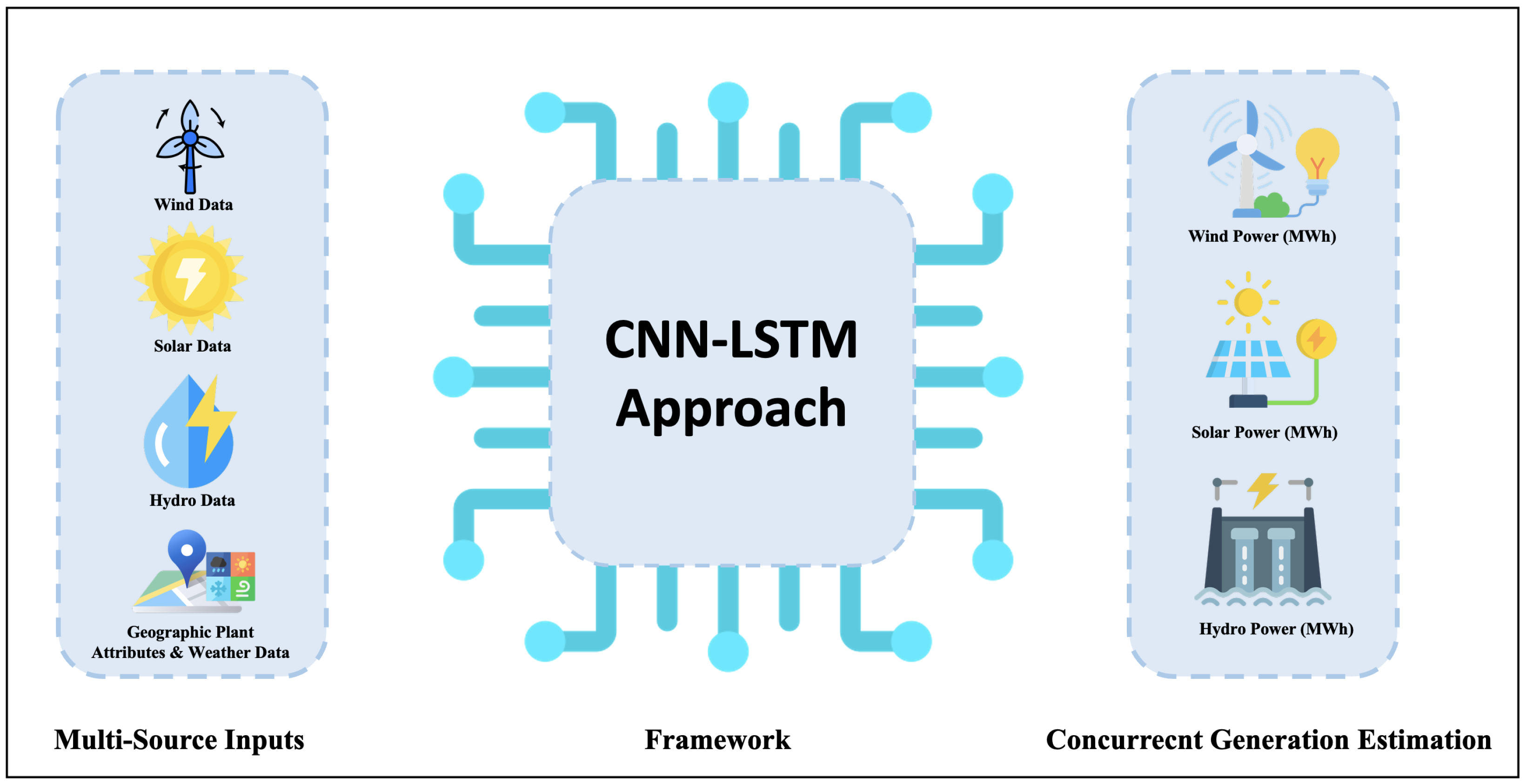
Conceptual framework of the CNN-LSTM approach for multi-source renewable energy estimation. The model integrates diverse inputs including solar, wind, hydro, and spatial weather data into a single deep learning architecture to produce concurrent generation estimates for each energy type.
Figure 1.
Conceptual framework of the CNN-LSTM approach for multi-source renewable energy estimation. The model integrates diverse inputs including solar, wind, hydro, and spatial weather data into a single deep learning architecture to produce concurrent generation estimates for each energy type.
Figure 2.
Summary of related studies (2024–2025). The studies listed in the table correspond to the following references: Abid et al. [
5], Nurhayati et al. [
6], Abirami et al. [
7], Sudasinghe et al. [
8], Ye et al. [
9], Jang et al. [
10], and Khan et al. [
11].
Figure 2.
Summary of related studies (2024–2025). The studies listed in the table correspond to the following references: Abid et al. [
5], Nurhayati et al. [
6], Abirami et al. [
7], Sudasinghe et al. [
8], Ye et al. [
9], Jang et al. [
10], and Khan et al. [
11].
Figure 3.
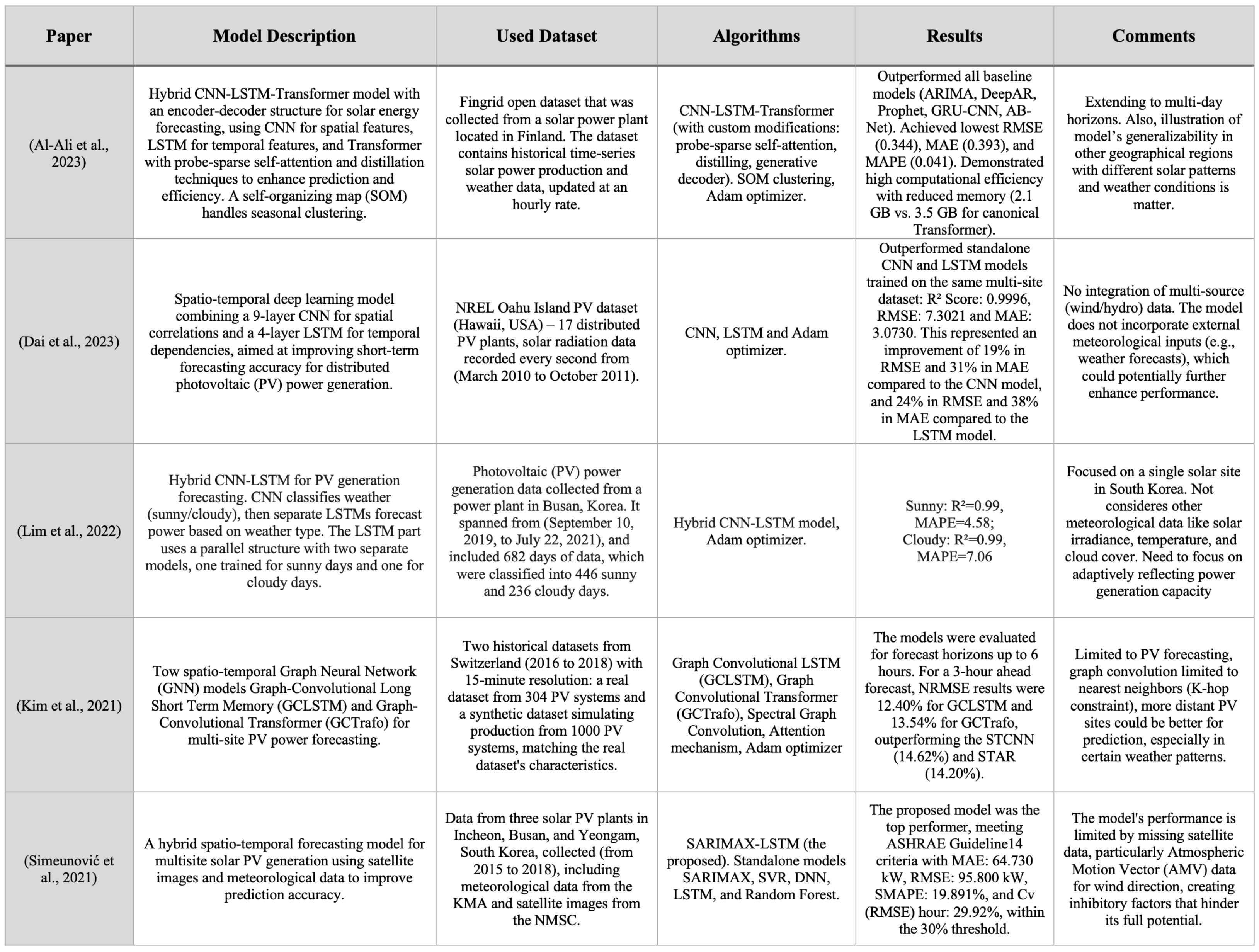
Summary of related studies (2021–2023). The studies listed in the table correspond to the following references: Al-Ali et al. [
12], Dai et al. [
13], Lim et al. [
14], Kim et al. [
16], and Simeunović et al. [
15].
Figure 3.
Summary of related studies (2021–2023). The studies listed in the table correspond to the following references: Al-Ali et al. [
12], Dai et al. [
13], Lim et al. [
14], Kim et al. [
16], and Simeunović et al. [
15].
Figure 4.
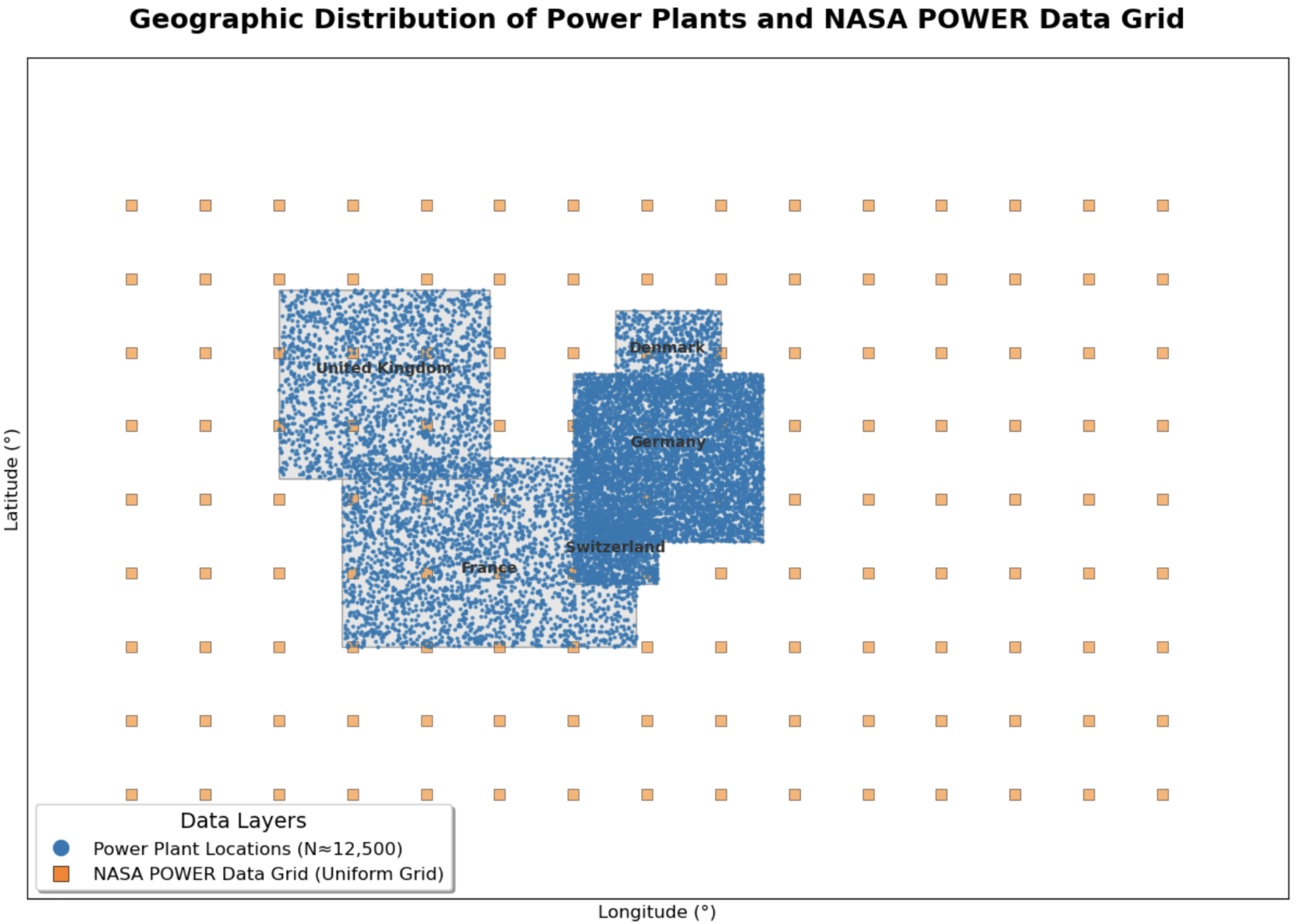
Geographic distribution of the power plant locations and the NASA POWER data grid used in this study. The dense blue points represent the locations of the 12,299 unique power plants, concentrated within the five study countries (United Kingdom, France, Germany, Switzerland, and Denmark). The sparse orange squares represent the uniform grid of the satellite-derived meteorological data. This visualization highlights the spatial mismatch that necessitates the use of the cKDTree algorithm for accurate feature matching.
Figure 5.
The S-shaped relationship between wind speed and the physics-informed Capacity Factor. This curve, generated using a hyperbolic tangent function, models the non-linear response of a wind turbine to varying wind speeds.
Figure 5.
The S-shaped relationship between wind speed and the physics-informed Capacity Factor. This curve, generated using a hyperbolic tangent function, models the non-linear response of a wind turbine to varying wind speeds.
Figure 6.
The proposed CNN-LSTM model architecture. The model features a two-branch design to process sequential weather data and static plant attributes in parallel. The outputs are concatenated and passed into a final prediction head to estimate the Capacity Factor.
Figure 6.
The proposed CNN-LSTM model architecture. The model features a two-branch design to process sequential weather data and static plant attributes in parallel. The outputs are concatenated and passed into a final prediction head to estimate the Capacity Factor.
Figure 7.
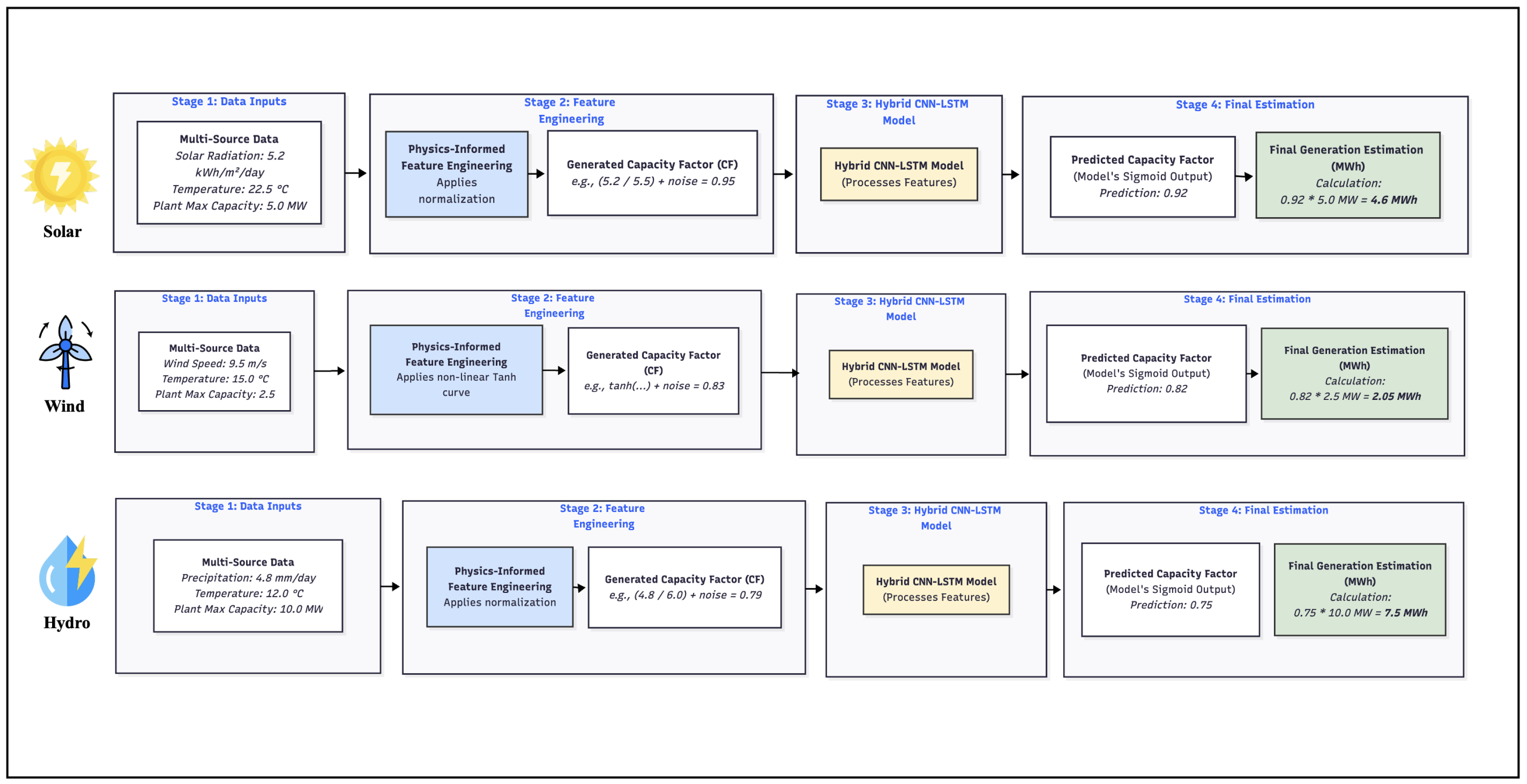
End-to-end workflow examples for Solar, Wind, and Hydro energy estimation. Each row demonstrates the four main stages of the proposed framework: (1) ingestion of source-specific spatio-temporal data; (2) application of physics-informed feature engineering to generate a normalized Capacity Factor; (3) processing through the unified hybrid CNN-LSTM model; and (4) conversion of the model’s predicted Capacity Factor into a final, real-world generation estimation in MWh.
Figure 8.
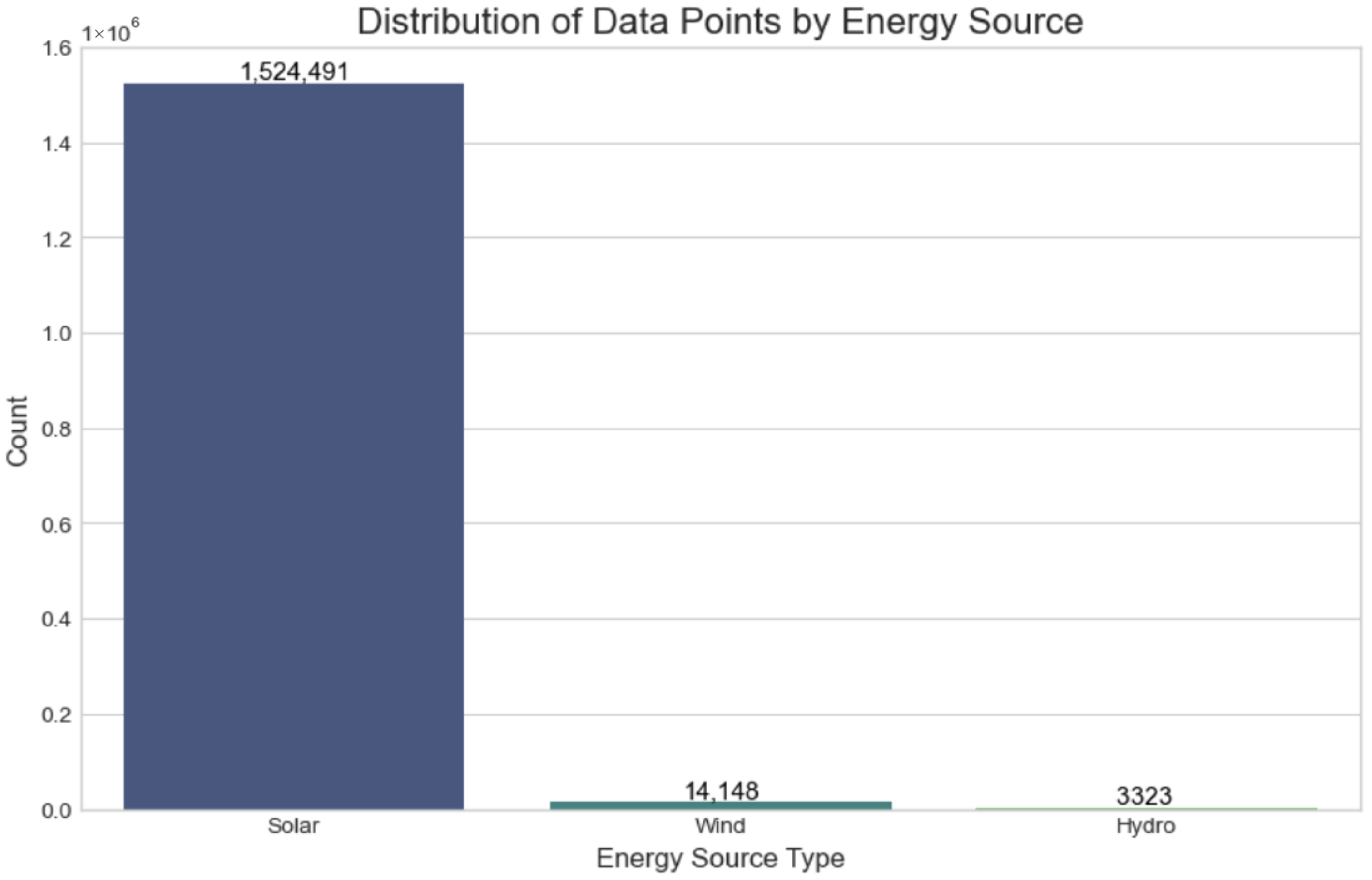
Distribution of the 1,541,962 data points by energy source, showing the significant imbalance with a predominance of solar records in the dataset.
Figure 8.
Distribution of the 1,541,962 data points by energy source, showing the significant imbalance with a predominance of solar records in the dataset.
Figure 9.
Correlation heatmap of the key numerical variables. A strong positive correlation is evident between temperature and solar radiation, while other features show weaker relationships, indicating their relative independence.
Figure 9.
Correlation heatmap of the key numerical variables. A strong positive correlation is evident between temperature and solar radiation, while other features show weaker relationships, indicating their relative independence.
Figure 10.
Forecast comparison of the first 100 test samples. The CNN-LSTM model (red) follows the actual generation (black) and baseline models, demonstrating its capability to capture rapid ramp-up and ramp-down events.
Figure 10.
Forecast comparison of the first 100 test samples. The CNN-LSTM model (red) follows the actual generation (black) and baseline models, demonstrating its capability to capture rapid ramp-up and ramp-down events.
Figure 11.
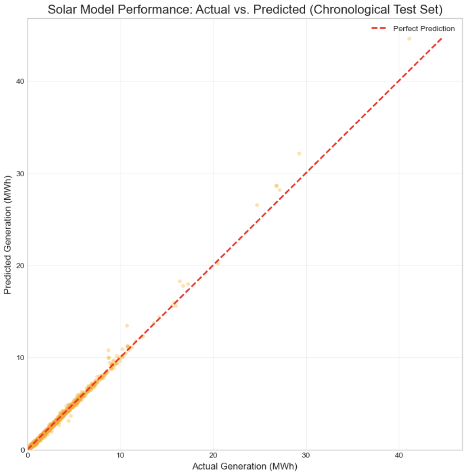
Actual vs. Predicted solar power generation on the chronological test set. The alignment along the diagonal confirms the model’s predictive accuracy.
Figure 11.
Actual vs. Predicted solar power generation on the chronological test set. The alignment along the diagonal confirms the model’s predictive accuracy.
Figure 12.
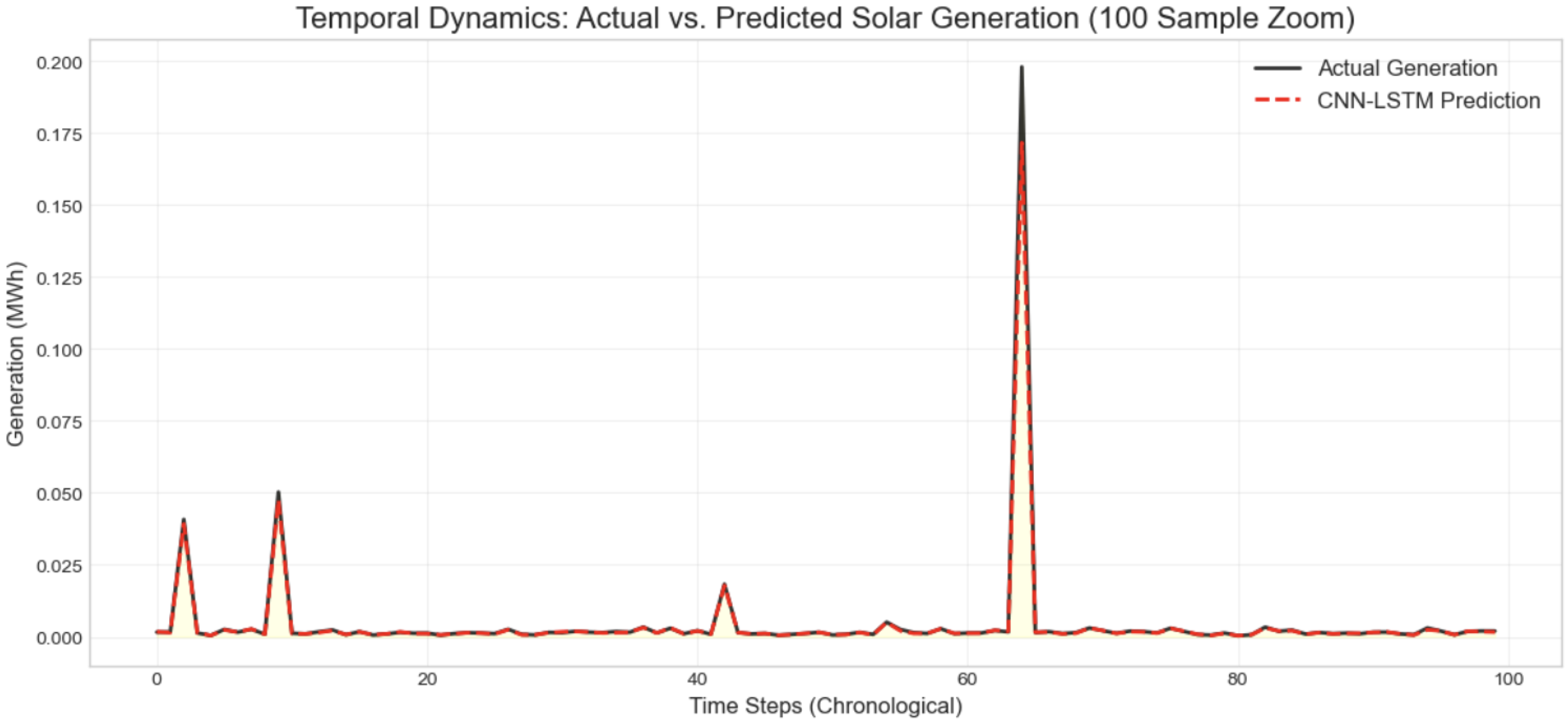
Temporal Dynamics: A 100-sample zoom of Actual vs. Predicted Solar Generation. The model accurately captures the intermittent nature of solar power, including the zero-generation periods during the night.
Figure 12.
Temporal Dynamics: A 100-sample zoom of Actual vs. Predicted Solar Generation. The model accurately captures the intermittent nature of solar power, including the zero-generation periods during the night.
Figure 13.
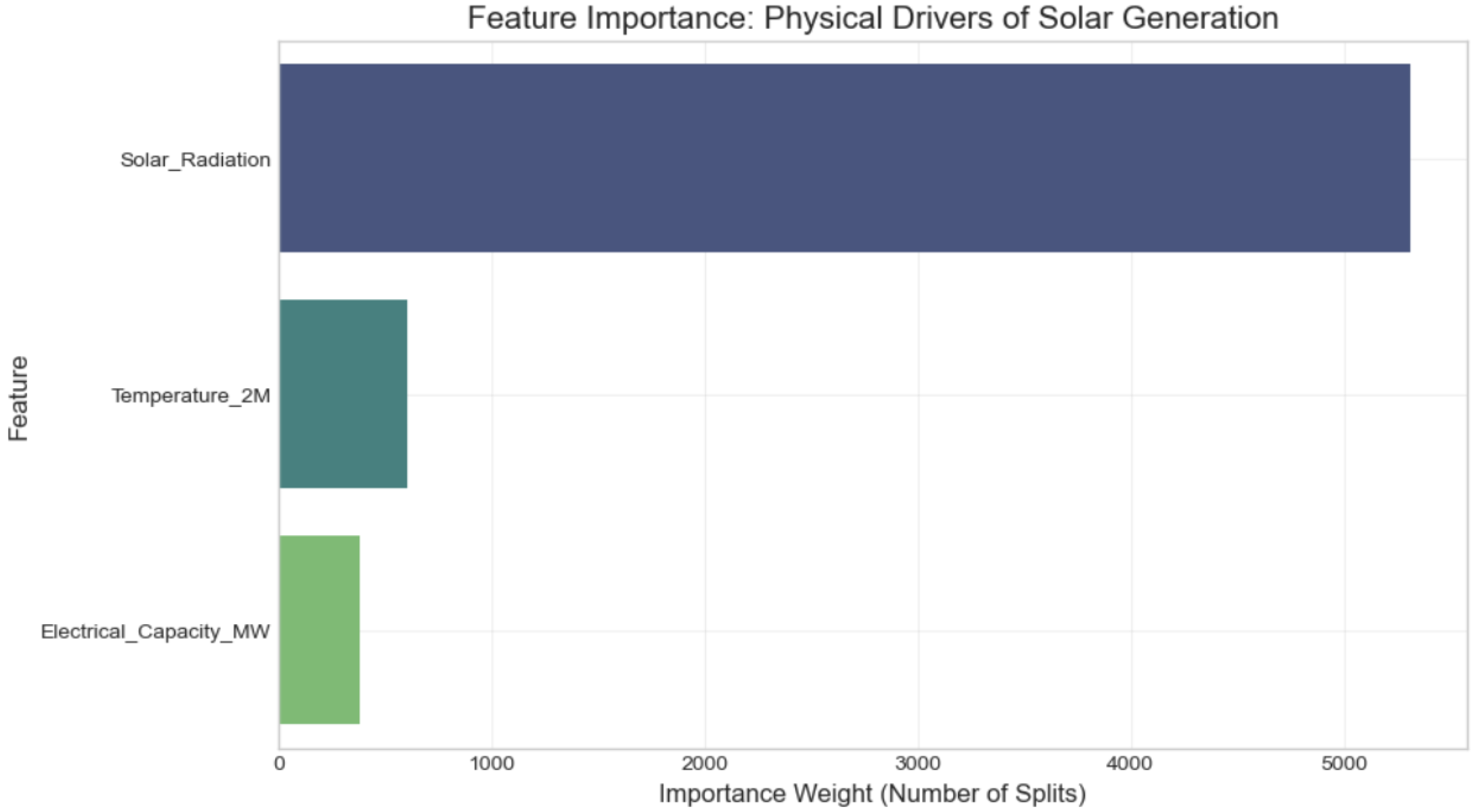
Feature Importance analysis for Solar Generation. The results confirm that Solar Radiation is the primary driver, validating the physical soundness of the dataset features.
Figure 13.
Feature Importance analysis for Solar Generation. The results confirm that Solar Radiation is the primary driver, validating the physical soundness of the dataset features.
Figure 14.
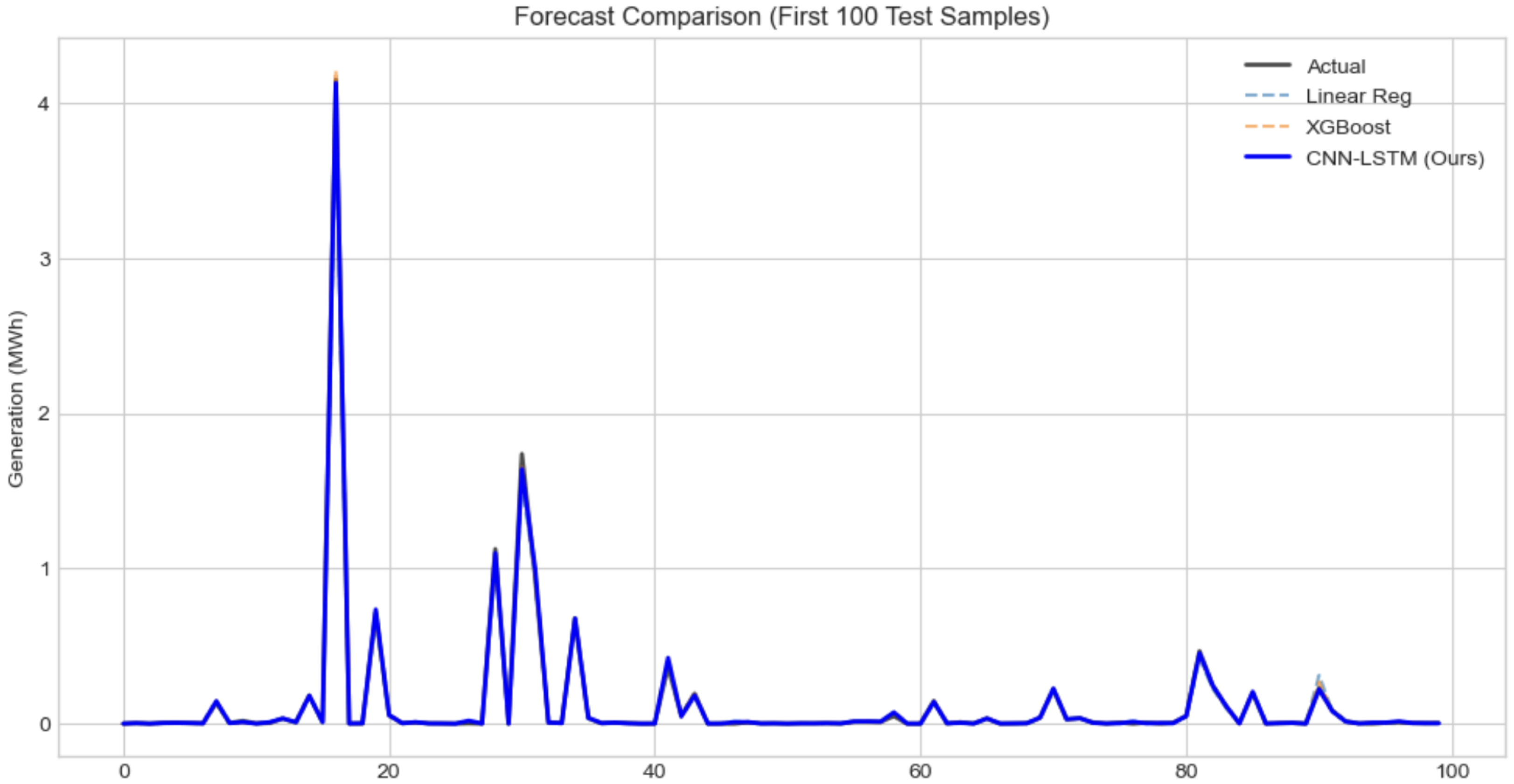
Forecast comparison for Wind Generation. The CNN-LSTM model successfully tracks the rapid, non-linear fluctuations of wind power, outperforming the baselines in capturing peak volatility.
Figure 14.
Forecast comparison for Wind Generation. The CNN-LSTM model successfully tracks the rapid, non-linear fluctuations of wind power, outperforming the baselines in capturing peak volatility.
Figure 15.
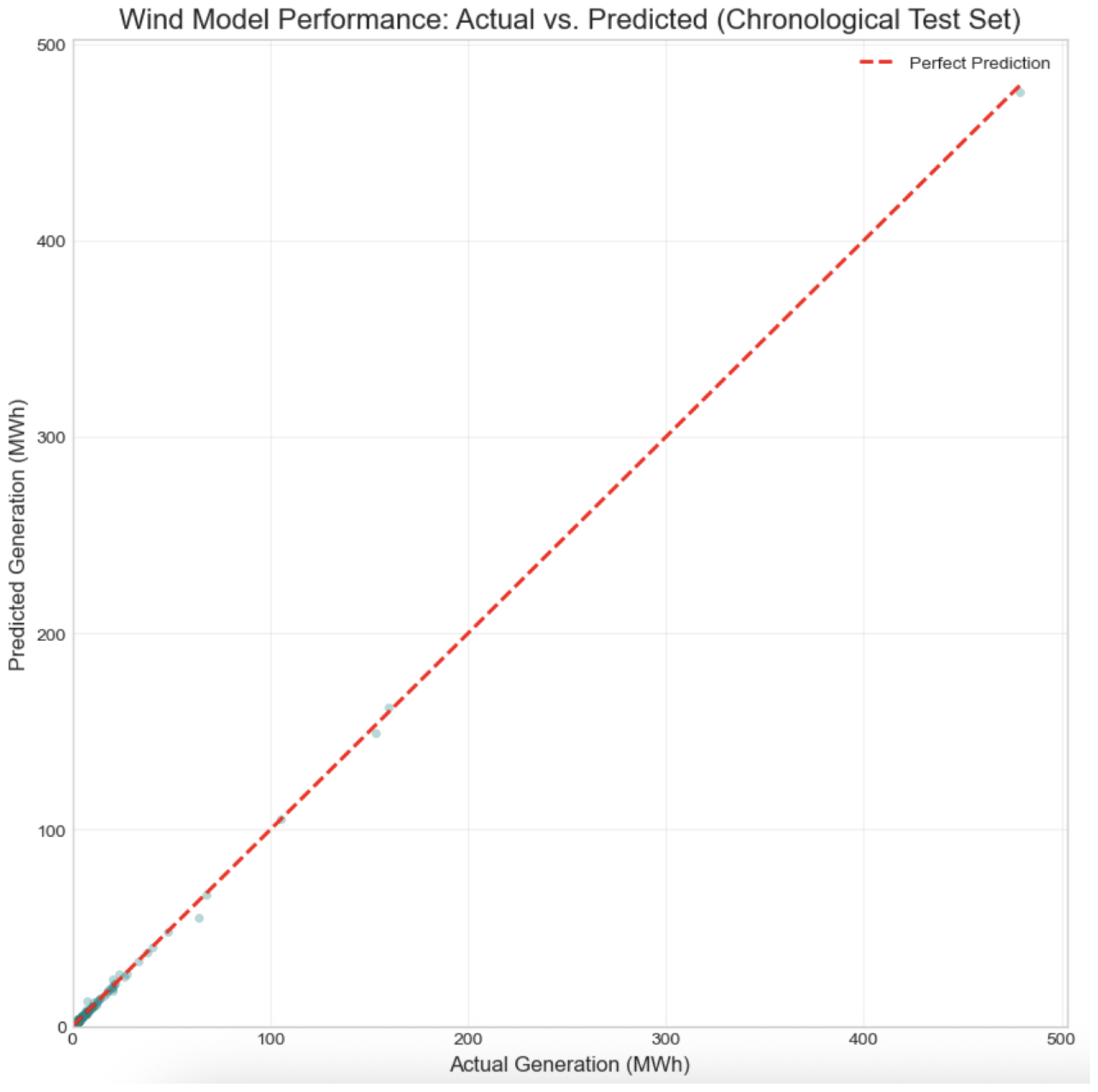
Actual vs. Predicted wind power generation. The strong linear alignment confirms that the physics-informed Tanh transformation successfully linearized the learning task for the neural network.
Figure 15.
Actual vs. Predicted wind power generation. The strong linear alignment confirms that the physics-informed Tanh transformation successfully linearized the learning task for the neural network.
Figure 16.
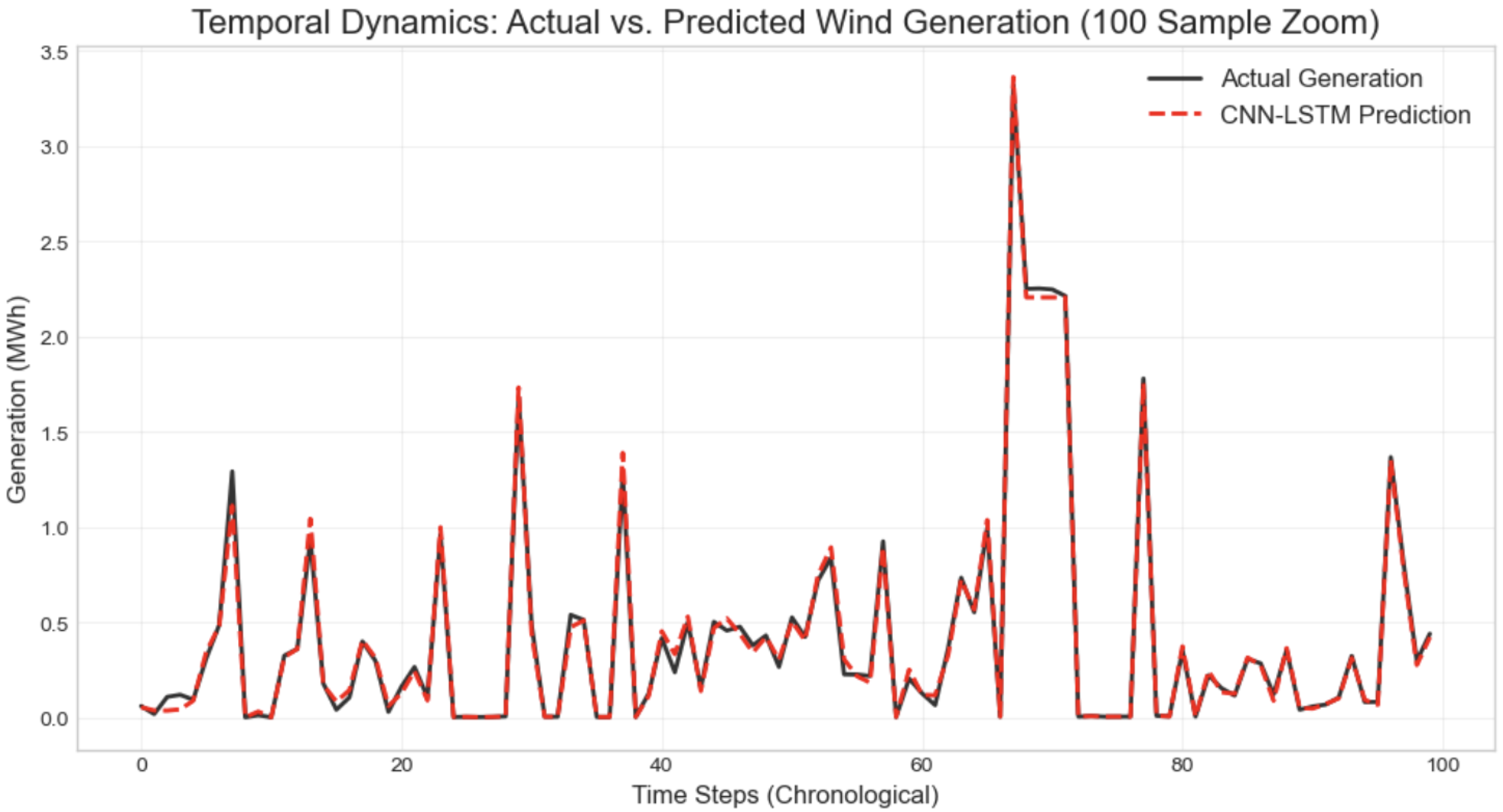
Temporal Dynamics: A zoom of Actual vs. Predicted Wind Generation. The model accurately captures the volatility and intermittency inherent in wind power.
Figure 16.
Temporal Dynamics: A zoom of Actual vs. Predicted Wind Generation. The model accurately captures the volatility and intermittency inherent in wind power.
Figure 17.
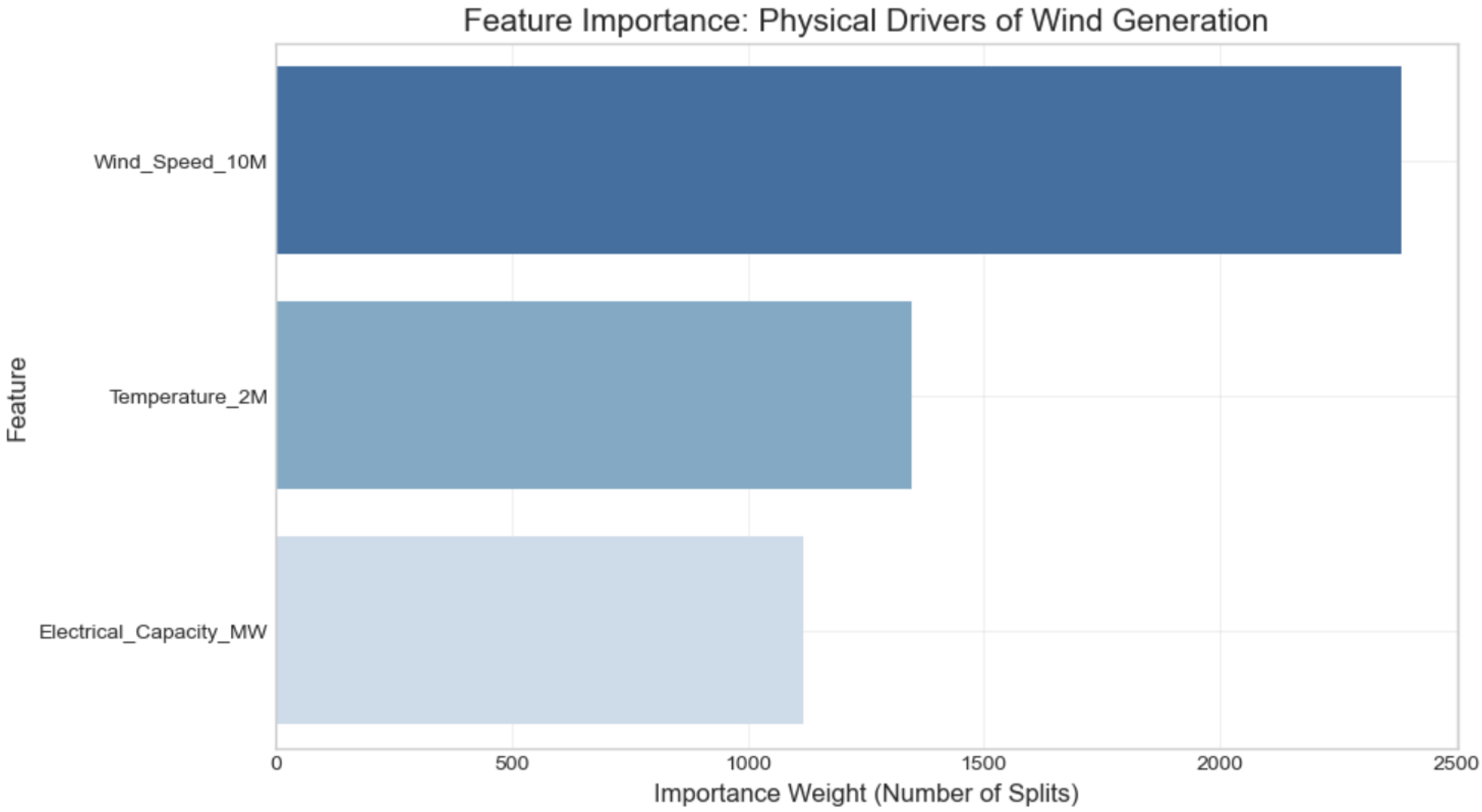
Feature Importance analysis for Wind Generation. The model correctly identifies Wind Speed as the primary physical driver, consistent with aerodynamic principles.
Figure 17.
Feature Importance analysis for Wind Generation. The model correctly identifies Wind Speed as the primary physical driver, consistent with aerodynamic principles.
Figure 18.
Forecast comparison for Hydro Generation. The model successfully identifies the timing of generation events, critical for reservoir management.
Figure 18.
Forecast comparison for Hydro Generation. The model successfully identifies the timing of generation events, critical for reservoir management.
Figure 19.
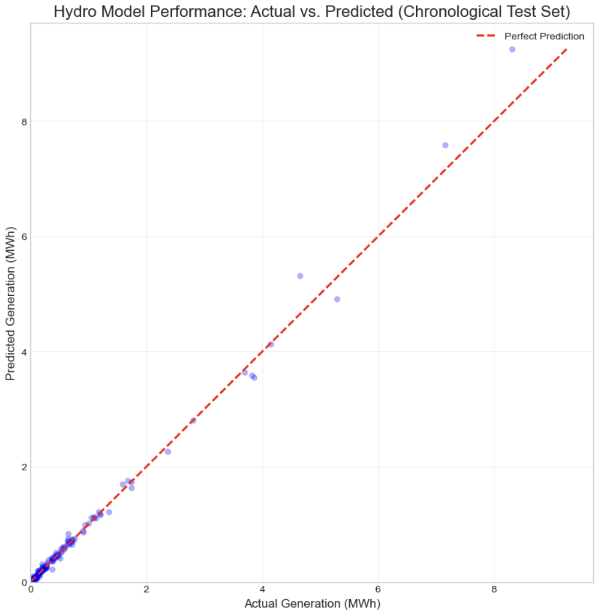
Actual vs. Predicted hydro power generation. The close correlation demonstrates the model’s effectiveness even on the smallest data subset.
Figure 19.
Actual vs. Predicted hydro power generation. The close correlation demonstrates the model’s effectiveness even on the smallest data subset.
Figure 20.
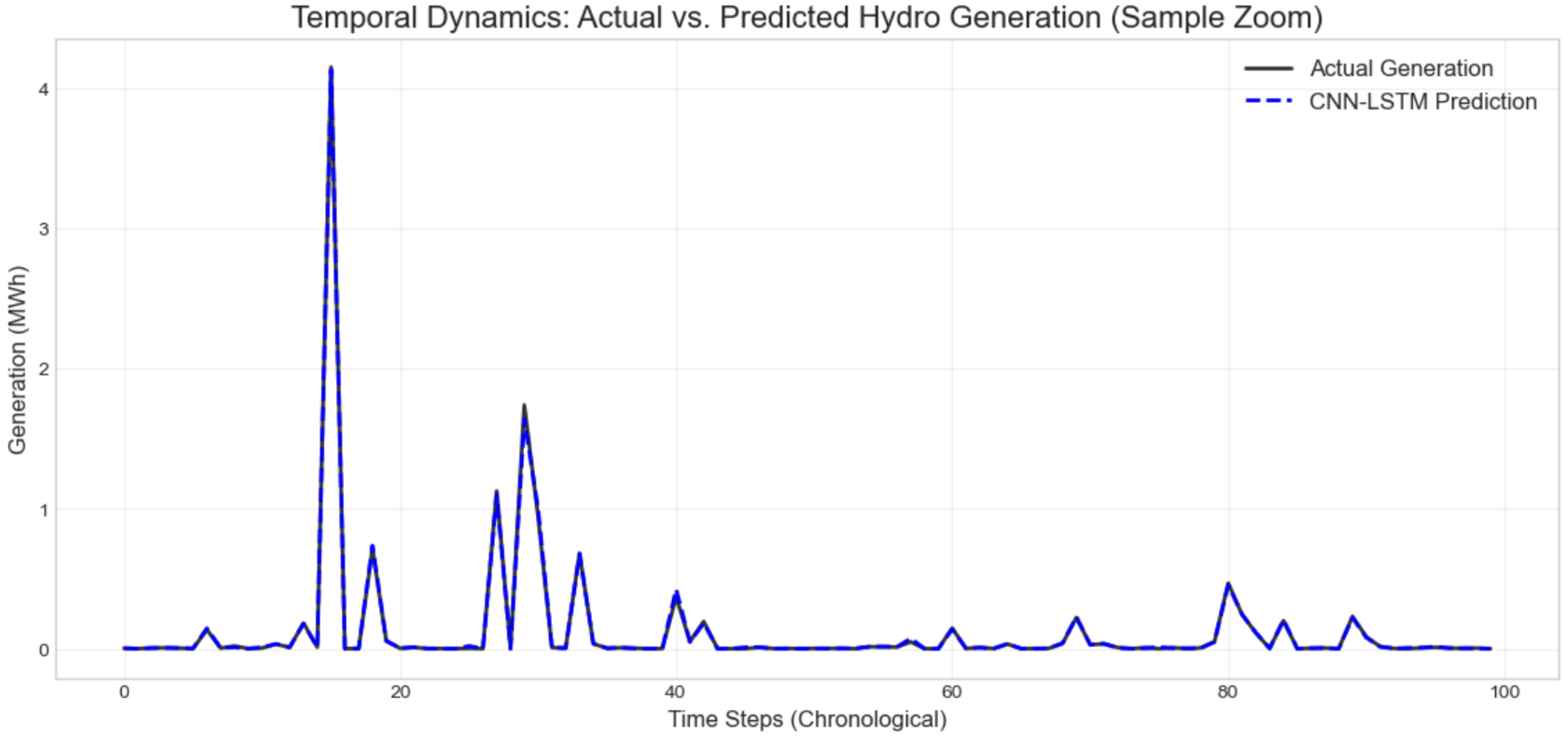
Temporal Dynamics: A zoom of Actual vs. Predicted Hydro Generation. The model accurately captures the timing of generation spikes driven by precipitation events.
Figure 20.
Temporal Dynamics: A zoom of Actual vs. Predicted Hydro Generation. The model accurately captures the timing of generation spikes driven by precipitation events.
Figure 21.
Feature Importance analysis for Hydro Generation. Precipitation is correctly identified as the dominant driver, validating the model’s physical interpretability.
Figure 21.
Feature Importance analysis for Hydro Generation. Precipitation is correctly identified as the dominant driver, validating the model’s physical interpretability.
Figure 22.
Model Accuracy () and Error (RMSE) comparison across all energy sources. The proposed CNN-LSTM model (green bar) demonstrates consistent high performance, matching baselines in linear tasks and surpassing them in complex non-linear tasks (Wind).
Figure 22.
Model Accuracy () and Error (RMSE) comparison across all energy sources. The proposed CNN-LSTM model (green bar) demonstrates consistent high performance, matching baselines in linear tasks and surpassing them in complex non-linear tasks (Wind).
Table 1.
Description of Key Raw Variables Used in the Study.
Table 1.
Description of Key Raw Variables Used in the Study.
| Variable Name | Description | Source |
|---|
| Power Plant Attributes |
| electrical_capacity | The maximum rated power output of the plant in Megawatts (MW). | OPSD [18] |
| lat, lon | The geographic latitude and longitude coordinates of the power plant. | OPSD [18] |
| energy_source_level_2 | The primary type of renewable energy source (Solar, Wind, or Hydro). | OPSD [18] |
| commissioning_date | The date on which the power plant was commissioned. | OPSD [18] |
| country | The two-letter country code where the plant is located. | OPSD [18] |
| Meteorological Data |
| T2M | Temperature at 2 m above the surface, in degrees Celsius. | NASA POWER [19] |
| WS10M | Wind speed at 10 m above the surface, in meters per second. | NASA POWER [19] |
| ALLSKY_SFC_SW_DWN | All-sky surface shortwave downward irradiance (total solar radiation), in kWh/m2/day. | NASA POWER [19] |
| PRECTOTCORR | Bias-corrected precipitation, in millimeters per day (mm/day). | NASA POWER [19] |
Table 2.
Spatio-Temporal Feature Matching Algorithm. This table outlines the procedural pipeline for associating each power plant with its nearest weather data point using the cKDTree algorithm for computationally efficient spatial querying.
Table 2.
Spatio-Temporal Feature Matching Algorithm. This table outlines the procedural pipeline for associating each power plant with its nearest weather data point using the cKDTree algorithm for computationally efficient spatial querying.
| Input | plant_data (DataFrame with plant ‘lat’, ‘lon’, ‘date’) weather_data (DataFrame with weather ‘lat’, ‘lon’, ‘date’)
|
| Output | |
| Algorithm | plant_coords = Get unique [lat, lon] pairs from plant_data weather_coords = Get unique [lat, lon] pairs from weather_data
// Build a KD-Tree for efficient lookups weather_tree = cKDTree(weather_coords)
// Query the tree for the nearest weather point index distances, indices = weather_tree.query(plant_coords, k=1)
// Retrieve coordinates of the nearest neighbors nearest_coords = weather_coords[indices] plant_data[‘matched_lat’] = nearest_coords[:, 0] plant_data[‘matched_lon’] = nearest_coords[:, 1]
// Merge datasets on date and matched coordinates merged_data = pd.merge(plant_data, weather_data, on=[‘date’, ‘matched_lat’, ‘matched_lon’]) Return merged_data
|
Table 3.
Layer-by-Layer Specification and Functional Description of the CNN-LSTM Architecture.
Table 3.
Layer-by-Layer Specification and Functional Description of the CNN-LSTM Architecture.
| Layer (Type) | Output Shape | Param # | Purpose |
|---|
| Block 1: Sequential Branch (Spatio-Temporal Processing) |
| Input_Seq | (None, 1, 2) | 0 | Receives sequential weather data (2 features, 1 time step). |
| Conv1D | (None, 1, 80) | 240 | Extracts local spatial/temporal patterns from weather inputs. |
| LSTM | (None, 80) | 51,520 | Models long-range temporal dependencies from the extracted features. |
| Dropout | (None, 80) | 0 | Regularization to prevent overfitting in the sequential branch. |
| Block 2: Static Branch (Attribute Processing) |
| Input_Static | (None, 1) | 0 | Receives static plant capacity data. |
| Dense | (None, 80) | 160 | Creates a non-linear representation of the static input. |
| Dropout_1 | (None, 80) | 0 | Regularization for the static branch. |
| Dense_1 | (None, 40) | 3240 | Further processes the static feature representation. |
| Block 3: Integration and Prediction Head |
| Concatenate | (None, 120) | 0 | Merges the feature vectors from the sequential and static branches. |
| Dense_2 | (None, 150) | 18,150 | Learns higher-level interactions from the combined features. |
| Dropout_2 | (None, 150) | 0 | Regularization for the prediction head. |
| Dense_3 | (None, 75) | 11,325 | Further refines the feature representation before output. |
| Block 4: Output Layer |
| Output (Dense) | (None, 1) | 76 | Produces the final prediction. Uses a ‘sigmoid’ activation to constrain the output to the [0, 1] range, matching the Capacity Factor. |
| Total Params | | 84,711 | |
| Trainable Params | | 84,711 | |
| Non-trainable Params | | 0 | |
Table 4.
Key Hyperparameters and Configurations Used for Model Training.
Table 4.
Key Hyperparameters and Configurations Used for Model Training.
| Parameter | Setting |
|---|
| Model Architecture |
| CNN Filters/LSTM Units | 80 |
| Dense Layer Units | 80, 40, 150, 75 |
| Activation Functions | ReLU (hidden), Sigmoid (output) |
| Dropout Rate | 0.4 |
| Training Configuration |
| Optimizer | Adam |
| Learning Rate | 0.0005 |
| Loss Function | Binary Cross-Entropy |
| Batch Size | 1024 (Solar), 512 (Wind), 64 (Hydro) |
| Epochs | 50–100 (with Early Stopping) |
| Early Stopping Patience | 5–10 epochs |
| Data Handling |
| Train-Test Split | Chronological (80% train, 20% test) |
| Feature Scaling | MinMaxScaler (range [0, 1]) |
Table 5.
Software and hardware tools used in the implementation.
Table 5.
Software and hardware tools used in the implementation.
| Category | Tool and Version |
|---|
| OS/Hardware | Apple MacBook Air (M1, 2020), 8 GB RAM |
| Language | Python 3.10 |
| Notebooks | Jupyter Notebook 7.3.2. |
| Visualization | Matplotlib 3.9, Seaborn 0.13.2 |
| Data Handling | Pandas 2.2.3, NumPy 1.26.4, SciPy |
| Machine Learning | scikit-learn 1.6.1, XGBoost 2.0.3 |
| Deep Learning | TensorFlow 2.18.0 (with Keras API) |
Table 6.
Performance Comparison of Solar Estimation Models (Test Set).
Table 6.
Performance Comparison of Solar Estimation Models (Test Set).
| Model | RMSE (MWh) | R2 Score |
|---|
| Linear Regression (Baseline) | 0.0098 | 0.9988 |
| XGBoost (Baseline) | 0.0097 | 0.9988 |
| Proposed CNN-LSTM | 0.0164 | 0.9967 |
Table 7.
A random sample of predictions for solar power generation (Test Set).
Table 7.
A random sample of predictions for solar power generation (Test Set).
| Sample Index | Actual (MWh) | Predicted (MWh) | Error (MWh) |
|---|
| 56,266 | 0.0062 | 0.0064 | −0.0003 |
| 256,361 | 0.0021 | 0.0020 | 0.0001 |
| 185,186 | 0.0013 | 0.0011 | 0.0002 |
| 184,360 | 0.0012 | 0.0013 | −0.0000 |
| 252,670 | 0.0010 | 0.0009 | 0.0001 |
| 274,176 | 0.0199 | 0.0198 | 0.0001 |
| 199,415 | 0.0034 | 0.0035 | −0.0001 |
| 93,433 | 0.0005 | 0.0005 | −0.0001 |
Table 8.
Performance Comparison of Wind Estimation Models (Test Set).
Table 8.
Performance Comparison of Wind Estimation Models (Test Set).
| Model | RMSE (MWh) | R2 Score |
|---|
| Linear Regression (Baseline) | 2.9180 | 0.9228 |
| XGBoost (Baseline) | 0.3328 | 0.9990 |
| Proposed CNN-LSTM | 0.2681 | 0.9993 |
Table 9.
A random sample of predictions for wind power generation (Test Set).
Table 9.
A random sample of predictions for wind power generation (Test Set).
| Sample Index | Actual (MWh) | Predicted (MWh) | Error (MWh) |
|---|
| 1025 | 0.0115 | 0.0388 | −0.0273 |
| 1413 | 0.2621 | 0.2178 | 0.0443 |
| 2238 | 1.9584 | 1.9651 | −0.0067 |
| 2771 | 0.1957 | 0.0784 | 0.1174 |
| 196 | 0.0022 | 0.0024 | −0.0002 |
| 1846 | 0.1032 | 0.0644 | 0.0388 |
| 322 | 1.3017 | 1.3025 | −0.0009 |
| 2554 | 0.5134 | 0.1705 | 0.3429 |
Table 10.
Performance Comparison of Hydro Estimation Models (Test Set).
Table 10.
Performance Comparison of Hydro Estimation Models (Test Set).
| Model | RMSE (MWh) | R2 Score |
|---|
| Linear Regression (Baseline) | 0.0518 | 0.9933 |
| XGBoost (Baseline) | 0.0273 | 0.9981 |
| Proposed CNN-LSTM | 0.0562 | 0.9922 |
Table 11.
A random sample of predictions for hydro power generation (Test Set).
Table 11.
A random sample of predictions for hydro power generation (Test Set).
| Sample Index | Actual (MWh) | Predicted (MWh) | Error (MWh) |
|---|
| 281 | 0.0000 | 0.0003 | −0.0003 |
| 286 | 0.0000 | 0.0002 | −0.0002 |
| 473 | 0.0019 | 0.0068 | −0.0050 |
| 227 | 0.0000 | 0.0008 | −0.0008 |
| 436 | 0.0003 | 0.0002 | 0.0001 |
| 360 | 0.0820 | 0.0754 | 0.0067 |
| 648 | 0.0126 | 0.0485 | −0.0359 |
| 465 | 0.0495 | 0.0484 | 0.0011 |
Table 12.
Consolidated Performance Summary for All Models (Chronological Test Set).
Table 12.
Consolidated Performance Summary for All Models (Chronological Test Set).
| Energy Source | Model | RMSE (MWh) | Score |
|---|
| Solar | Linear Regression | 0.0098 | 0.9988 |
| | XGBoost | 0.0097 | 0.9988 |
| | Proposed CNN-LSTM | 0.0164 | 0.9967 |
| Wind | Linear Regression | 2.9180 | 0.9228 |
| | XGBoost | 0.3328 | 0.9990 |
| | Proposed CNN-LSTM | 0.2681 | 0.9993 |
| Hydro | Linear Regression | 0.0518 | 0.9933 |
| | XGBoost | 0.0273 | 0.9981 |
| | Proposed CNN-LSTM | 0.0562 | 0.9922 |
Table 13.
Analytical Comparison of the Proposed Framework with Traditional Methods.
Table 13.
Analytical Comparison of the Proposed Framework with Traditional Methods.
| Capability | Traditional Methods (e.g., ARIMA, XGBoost) | Proposed Spatio-Temporal CNN-LSTM |
|---|
| Non-Linearity | Limited. ARIMA assumes linearity; XGBoost handles non-linearity but lacks physics awareness. | The deep architecture with ReLU activations and Tanh target scaling inherently models complex, non-linear functions (e.g., Wind). |
| Spatial Context | Typically uses single or averaged weather data points, ignoring local variations. | The Conv1D layer extracts spatial patterns, and the cKDTree preprocessing ensures hyper-local weather data is used. |
| Temporal Context | Limited. ARIMA captures basic auto-correlation, while XGBoost has no innate sequence awareness. | The LSTM layer is specifically designed to learn patterns from sequential data, capturing time-dependent dynamics. |
| Physics-Informed | Requires extensive manual feature engineering; struggles with domain concepts. | The Tanh-based Capacity Factor is a built-in, physics-informed feature that guides the model towards realistic physical constraints. |
| Generalizability | A model tuned for one energy source often requires re-engineering for others. | The single, unified architecture performed exceptionally well across three different energy sources and five countries. |
