How Urban Distance Operates: A Nonlinear Perspective on Talent Mobility Intention in the Yangtze River Delta

Abstract

Based on micro-level job seeker data from 41 cities in China’s Yangtze River Delta, this study employs threshold regression to examine how inter-city distance influences talent mobility. The results reveal that distance exerts a negative impact on mobility intention and moderates the relationship between a destination’s economic level and mobility. Notably, significant threshold effects are identified at 164.1 km and 271.5 km, delineating three spatial regimes. Short-distance flows (<164.1 km) show the highest intensity, driven by strong economic incentives and high mobility. In contrast, medium-distance flows (164.1–271.5 km) prove least attractive due to offsetting effects, while long-distance flows (>271.5 km) rebound slightly as talent selectively targets major economic hubs, with distance exhibiting only weak inhibition. Crucially, these nonlinear patterns remain robust after addressing endogeneity concerns via the 2SLS method, substituting spatial distance with temporal distance, and controlling for housing prices and cultural factors. Heterogeneity analysis further indicates that individuals with bachelor’s degrees, those above age 30, and talent in labor-intensive industries exhibit greater sensitivity to distance. Conversely, knowledge-intensive sectors and top-tier economic cities demonstrate broader spatial tolerance and stronger cross-regional attraction capabilities. These findings provide a quantitative basis for developing differentiated regional talent policies.

1. Introduction

China is undergoing a large-scale, multi-tiered wave of talent mobility. According to the Seventh National Population Census, the size of China’s floating population has reached 376 million, with a steadily increasing proportion of individuals possessing specialized knowledge and skills. This demographic shift has transcended mere labor migration to become a critical determinant of urban sustainability. The efficient spatial allocation of such high-quality human capital is essential for fostering innovation ecosystems and ensuring the long-term economic and social vitality of urban regions. As the most economically dynamic region in China, the Yangtze River Delta is witnessing intensifying competition for talent, reflecting a strategic consensus that talent retention is the cornerstone of sustainable regional development. Within this context, geographical distance, as a key factor influencing talent mobility intentions, has long been a focus of academic inquiry. As early as the 1960s, the ‘push–pull’ theory proposed that distance may function as a barrier to migration [1], a perspective widely corroborated by subsequent studies regarding the inhibitory effect of distance on mobility intention. However, in terms of the underlying mechanisms, most existing research has adopted a linear perspective, largely overlooking the complex dynamics of talent migration under geographical constraints.

Talent migration is ultimately driven by the goal of maximizing returns on human capital. Relocating to cities with greater economic capacity typically offers the potential for higher income and enhanced career development opportunities. Conversely, greater distance significantly elevates migration costs, including the loss of familial support, the disruption of social networks, and the risks associated with cultural adaptation. Variations in geographical distance lead to complex, nonlinear changes in both perceived benefits and costs. Consequently, the mobility decisions of job seekers essentially represent a dynamic trade-off between these factors. This mechanism suggests that the influence of distance on mobility intention may not be adequately captured by a simple linear inhibitory relationship. Nevertheless, existing studies have yet to fully elucidate how geographical distance shapes job seekers’ cost–benefit calculus or to establish clear quantitative thresholds for what constitutes ‘short’ versus ‘long’ distance.

Building on this foundation, this study utilizes micro-level data on job seekers from 41 cities in the Yangtze River Delta and employs a threshold regression model to empirically address the following questions: (1) Does inter-city distance exert a nonlinear threshold effect on talent mobility intention? (2) How does geographical distance influence the costs and benefits perceived by job seekers? The potential marginal contributions of this research are twofold: (1) It elucidates the mechanisms by which a destination’s economic level and migration distance function across varying distance intervals, thereby enriching talent mobility theories by considering multiple distinct dimensions of heterogeneity, including education level, age, sector, and city economic hierarchy. (2) By quantifying distance thresholds through an empirical model, it transforms the abstract concepts of ‘short’ and ‘long’ distance into actionable parameters for governance, providing a quantitative basis for formulating targeted talent policies.

2. Literature Review

2.1. Factors Influencing Talent Mobility

The ‘push–pull theory’ has served as a foundational framework for examining talent mobility in previous research. Bogue [2] initially proposed that population movement aims to improve living conditions, where favorable factors in destination areas act as ‘pull’ forces and unfavorable conditions in original areas serve as ‘push’ forces. The outcome of migration is determined by the relative strength of these forces. Lee [1] further refined this theory by introducing the concept of intermediate obstacles, including distance, physical barriers, linguistic and cultural differences, and migrants’ subjective valuations of these factors.

In recent years, research on the factors influencing talent mobility has become increasingly diversified. City economic development [3] and amenities [4] remain recognized as significant determinants of talent inflow. Studies by Ding et al. [5] and Jiang et al. [6] both indicate that economic factors are the primary consideration for university graduates when selecting a city. Jia and Guo [7] observed that population migration in central and western China predominantly gravitated toward administrative centers, with floating population hotspots largely concentrated in provincial capitals and economically dynamic regions. Xie et al. [8] found that, in addition to economic factors, urban amenities, such as consumer and cultural facilities, and social atmosphere also contribute to attracting returnees. However, some studies argue that the role of pure economic attractiveness has diminished. Wang et al. [9] noted that economic incentives are becoming less decisive in destination choices, as people increasingly prefer cities that offer better employment opportunities and settlement support. Scholars have also adopted more specific and micro-level perspectives, examining how industrial transfer [10], housing policies [11], air pollution [12], environmental inequality [13], and even talent categories [14] influence talent mobility to varying degrees.

2.2. Geographical Distance and Talent Mobility

Although Cairncross [15] claimed that the communications revolution has profoundly ‘shrunk the world,’ effectively heralding the ‘death of distance’ as an economic and social constraint, numerous studies have consistently shown that distance remains a significant factor influencing individual decisions in areas such as learning collaboration [16] and job seeking [17]. Regarding migration distance, Gu [18] reveals that distance friction and social ties still influence both highly educated and less educated migrants. Liu and Li [10] found that most cities exhibit a positive migration distance decay parameter, indicating that the number of migrants declines as distance increases. Notably, the Yangtze River Delta region demonstrates a relatively high distance decay parameter. Halás et al. [19] observed that in the Czech Republic, migration flows of up to 50 km accounted for the majority (70.8%) of moves between municipalities, with shorter distances of 15 km and 25 km contributing 39.2% and 55.7% of flows, respectively. Subsequent research further confirmed that short-distance migration in the Czech Republic is characterized by an upper distance limit of approximately 50 km [20].

As research advances, scholars have begun to examine the interaction between factors such as economics, amenities, and geographical distance, finding that the influence of geographical distance on talent mobility may be nonlinear. Shi et al. [21] demonstrate the multidimensional nature of nonlinear push–pull effects, showing that economic and employment factors exert stronger pull effects at the destination than push effects at the origin, whereas the opposite holds for factors related to living environment and gender differences. Na and Liu [22] found that geographical distance has a strong negative impact on talent mobility, though this effect is mitigated in cities with stronger academic or economic capacity. Zhao et al. [23] revealed that migration does not decay linearly with distance but rather follows a nonlinear pattern in Shenzhen, China. This nonlinear relationship reflects the dynamic interplay between costs and opportunities and the trade-offs involved in migration decision-making.

The existing literature demonstrates a substantial body of research on talent mobility, with scholars having extensively analyzed its influencing factors. However, regarding the specific impact of geographical distance on talent flows, two aspects warrant further investigation: First, the trade-off between advantages and disadvantages in talent migration, particularly under different distance conditions, requires further discussion. Second, although prior research has acknowledged the role of inter-city distance in talent mobility, there is a lack of granular analysis, especially in quantifying distance thresholds, which limits its practical applicability as a concrete policy reference.

3. Research Design

3.1. Research Hypothesis

Early theoretical work, notably by [1], proposed that geographical distance acts as a deterrent to population movement. This view remains prevalent in contemporary scholarship, where a consensus generally holds that inter-city distance exerts a significant negative impact on talent mobility. Specifically, the mechanisms through which inter-city distance influences talent mobility intention manifest primarily in the following aspects:

1. Attachment to specific locales, such as one’s birthplace, educational institution, or family location. Individuals often develop strong emotional bonds with places associated with significant life events, emotional experiences, and identity formation. These locales carry profound personal memories and emotional weight. Numerous studies have documented migrants’ preferences for relocating to areas where they have kinship ties [24,25] or pre-existing place attachment [4,26]. This tendency is particularly pronounced among individuals with strong localist sentiments, a characteristic often observed in Chinese society. Such emotional connections reinforce the role of proximate spaces as the primary sphere of social interaction, thereby fostering a distinct preference for short-distance migration among talented individuals.

2. Costs associated with the loss of social and professional networks represent a critical consideration in migration decisions. Long-term residence and employment in a city allow individuals to accumulate extensive social resources, including colleagues, friends, and professional partners. Within China’s relationship-oriented society (guanxi), such networks provide not only emotional support but also generate valuable career opportunities. In a familiar environment, it is easier to establish trust and collaborative relationships, thereby reducing transaction costs and enhancing work efficiency. For instance, Haug [27] finds that social capital at the destination encourages plans to emigrate, while social ties in the current place of residence deter return migration. Similarly, Jin et al. [28] argue that support from family, friends, teachers, and classmates helps first-tier cities attract university graduates. Crucially, shorter distances facilitate the maintenance of existing social networks, whereas long-distance migration tends to weaken or sever these connections, requiring substantial time and effort to rebuild them in a new location.

3. Adjustments to cultural practices and lifestyle habits. Different cities possess distinct cultural backgrounds and local customs that shape residents’ values and daily behaviors. Long-distance mobility may expose individuals to dialect barriers [29], unfamiliar food, climatic differences, and varying holiday traditions, all of which can negatively affect living comfort and quality of life. When migration occurs within a shorter distance, these challenges can be significantly mitigated. Based on the above analysis, the following hypothesis is proposed:

Hypothesis 1.

Talent mobility intention is negatively correlated with inter-city distance.

Neoclassical migration theory [30,31,32,33] posits that the decision to migrate stems from a rational cost–benefit calculation. While economic gains constitute a primary benefit of migration, geographical distance often plays a decisive role in determining the associated costs. Wang et al. [34] found that migration decisions in China result from a rational trade-off between expected salary and relocation costs. Similarly, Bjerke and Mellander [35] demonstrate that the prospect of achieving higher income is a key motivator for talent migration in Sweden. Although cities with greater economic capacity can offer higher potential returns, increasing distance forces migrants to bear significant marginal costs, such as those related to transportation, time, and information search, while also confronting heightened risks related to social network disruption and cultural adaptation in the new city. Consequently, when economic attractiveness is held constant, greater inter-city distance can erode the net benefits of mobility and suppress the willingness to move. This leads to the following hypothesis:

Hypothesis 2.

Inter-city distance negatively moderates the impact of a destination’s economic level on talent mobility intention.

Building upon the cost–benefit framework, a growing body of research highlights the complex, nonlinear interplay between geographical distance and economic factors [21,22,23]. For example, Meng et al. [36] found that high-speed rail significantly influences employment in neighboring areas. The relative benefits and costs accessible to talent are highly sensitive to geographical scale. Shorter distances typically afford greater cultural and lifestyle proximity, alongside more resilient familial and social networks. As distance increases, these comparative advantages diminish, while monetary and psychological costs of mobility rise substantially. This dynamic trade-off suggests that the mechanisms through which economic disparities influence talent mobility are not uniform but are instead moderated by discrete distance intervals. The influence of an inter-city destination’s economic level on talent mobility may therefore exhibit distinct nonlinear characteristics across different geographical thresholds.

Hypothesis 3.

A threshold effect characterizes the relationship between inter-city distance and talent mobility intention in the context of a destination’s economic level.

Studies by Rezaei and Mouritzen [37] and MacLachlan and Gong [38] underscore the pivotal role of Chinese-style social networks (guanxi) and familial ties, respectively, in shaping talent mobility decisions. Inter-city distance directly determines commuting feasibility and time, which in turn governs the frequency of interaction with original social networks and family. At shorter distances, frequent daily or weekly commuting allows individuals to readily access support from family and existing professional circles, substantially lowering the psychological costs and adaptation risks of relocation. This mitigating effect intensifies as distance decreases. However, once distance exceeds a critical threshold, commuting frequency drops precipitously, shifting to monthly or even quarterly patterns. Beyond this point, further increases in distance no longer yield significant reductions in commuting frequency. Consequently, the relative weight of distance in the migration decision diminishes, and talent begins to evaluate potential destinations more comprehensively, prioritizing economic benefits, total migration costs, and overall urban livability. This behavioral shift implies that across varying distance intervals, the effect of migration distance on talent mobility intention is likely nonlinear. Thus, the following hypothesis is proposed:

Hypothesis 4.

A threshold effect exists in the influence of inter-city distance on talent mobility intention.

3.2. Research Methods

A standard ordinary least squares (OLS) regression was employed to examine the impact of inter-city distance on talent mobility intention. The econometric model is specified as follows:

$$\begin{array}{ll}{Intension}_{ij}={\beta }_0+{\beta }_1{Distance}_{ij}& +{\beta }_2{ln\_GDP}_j+{\beta }_3{ln\_Income}_j+\\ & +{\beta }_{4}Structur{e}_j+{\beta }_{5}Educatio{n}_j+{\beta }_{6}Sn+v_{ij}\end{array}$$

(1)

where Intention_ij represents the talent mobility intention from city i to city j, Distance_ij denotes the distance between city i and city j, ln_GDP_j, ln_Income_j, l n_Structure_j, Education_j, and Sn are control variables representing a destination’s economic level, income level, industrial structure, and education level, and whether the place of residence and the inflow destination are within the same province, respectively. Subsequently, an interaction term between inter-city distance and economic level (Distance_ij × ln_GDP_j) was incorporated into the model to examine the moderating effect of distance. The model is specified as follows:

$$\begin{array}{ll}{Intension}_{ij}& ={\beta }_0+{\beta }_{1}Distanc{e}_j+{\beta }_{2}ln\_GD{P}_j+{\beta }_{3}Distanc{e}_{ij}\times ln\_GD{P}_j\\ & +{\beta }_{4}ln\_Incom{e}_j+{\beta }_{5}Structur{e}_j+{\beta }_{6}Educatio{n}_j+{\beta }_{7}Sn+v_{ij}\end{array}$$

(2)

‘Short’ and ‘long’ are defined as two turning points of inter-city distance. First, we test whether the first threshold and the second threshold are significant and calculates the threshold values. Then, the original sample is divided into different intervals based on the threshold values for regression analysis to estimate the coefficients of the variables in each interval. The threshold model for a destination’s economic level is specified as follows:

$$\begin{array}{c}Intensio{n}_{ij}={\beta }_0+{\beta }_{1}Distanc{e}_{ij}+{\beta }_{2}ln\_GD{P}_j\times I\left(distance\le {\gamma }_1\right)\\ +{\beta }_{3}ln\_GD{P}_j\times I\left({\gamma }_1<distance\le {\gamma }_2\right)+{\beta }_{4}ln\_GD{P}_j\times I\left(distance>{\gamma }_2\right)\\ +{\beta }_{5}ln\_Incom{e}_j+{\beta }_{6}Structur{e}_j+{\beta }_{7}Educatio{n}_j+{\beta }_{8}Sn+v_{ij}\end{array}$$

(3)

where I(⋅) is an indicator function that takes the value 0 when the expression in parentheses is false and 1 otherwise. ${\gamma }_1$ and ${\gamma }_2$ represent the first threshold value and the second threshold value, respectively. In practice, the value of ${\gamma }_1$ is estimated first, and then the second threshold value ${\gamma }_2$ is estimated while keeping the first threshold value fixed. The model for testing the threshold effect of inter-city distance on the relationship between distance and talent mobility intention follows a similar specification.

3.3. Data Source

3.3.1. Study Area

The Yangtze River Delta, located on the eastern coast of China, is one of the nation’s most economically dynamic, open, and innovative regions, and correspondingly exhibits the highest frequency of talent mobility. This study focuses on 41 cities within this region, comprising the following:

One municipality: Shanghai.

Thirteen cities in Jiangsu province: Nanjing (provincial capital), Wuxi, Xuzhou, Changzhou, Suzhou, Nantong, Lianyungang, Huai’an, Yancheng, Yangzhou, Zhenjiang, Taizhou, and Suqian.

Eleven cities in Zhejiang province: Hangzhou (provincial capital), Ningbo, Wenzhou, Shaoxing, Huzhou, Jiaxing, Jinhua, Quzhou, Zhoushan, Taizhou, and Lishui.

Sixteen cities in Anhui province: Hefei (provincial capital), Wuhu, Ma’anshan, Tongling, Chizhou, Anqing, Xuancheng, Chuzhou, Bengbu, Huaibei, Huainan, Suzhou, Fuyang, Bozhou, Lu’an, and Huangshan.

The geographical distribution of these 41 cities within the Yangtze River Delta is shown in Figure 1.

3.3.2. Dependent Variable

The dependent variable in this study is talent mobility intention. While previous research has relied on employment destination records of university graduates [5], the China Migrant Dynamic Monitoring Survey [25], and national population sample surveys [39], this study utilizes data from professional social networking platforms to construct a measure of talent mobility. Online job-seeking platform data have gained increasing recognition in studies of talent mobility due to their objectivity and representativeness [8,9]. The specific procedures adopted are as follows:

High-level talent is defined as individuals with at least a bachelor’s degree. On the 51job platform, residence cities and desired job cities were specified. Data were collected in early January 2025 to include job seekers active within the preceding six months, resulting in residence-intended destination records. For example, a query for Shanghai to Nanjing returned 19,900, indicating that 19,900 job seekers whose residence was Shanghai had posted resumes targeting Nanjing as their desired work location within the past six months.

Records where the residence city and intended destination were the same were excluded from the talent mobility count, as no inter-city movement was involved. After this exclusion, 1640 valid records were obtained. To mitigate bias arising from varying city sizes, talent mobility intention was expressed as the number of job seekers per 100,000 registered population of the residence city, calculated by dividing the number of job seekers by the household registration population of the residence city. The spatial differentiation of GDP and talent mobility intention across the 41 cities is shown in Figure 2.

3.3.3. Independent Variable

The independent variable is the geographical distance between cities, calculated based on their longitude and latitude coordinates.

3.3.4. Control Variables

Control variables include the following: (1) Economic level. Talent mobility is significantly driven by the economic capacity of the inflow city. This variable is measured as the logarithm of the GDP of the destination city. (2) Income level. This is represented by the logarithm of the per capita disposable income of the destination city. (3) Industrial structure. This is measured according to the proportion of the tertiary industry. (4) Education level. This is captured by the number of secondary school teachers per 10,000 registered population in the destination city. (5) Same-province dummy. This is manually set to 1 if the residence city and destination city belong to the same province, and 0 otherwise. Relevant variables and data sources are summarized in

Table 1. Variable description.

Variable	Description	Data Source
Intention	Talent mobility intention	51job platform
Distance	Inter-city distance	National Geomatics Center of China
Ln_GDP	Economic level	Prefecture-level City Statistical Yearbooks
Ln_Income	Income level	Prefecture-level City Statistical Yearbooks
Structure	Industrial structure	Prefecture-level City Statistical Yearbooks
Ln_ed	Education level	Prefecture-level City Statistical Yearbooks
Sn	Same-province dummy	Manually set

.

4. The Impact of Inter-City Distance on Talent Mobility Intention

4.1. Descriptive Statistical and Correlation Analysis

Descriptive statistics and Pearson correlation analyses were conducted using Stata 16.

Table 2. Descriptive statistics.

Variable	Mean	Std.	Min	Max
Intention	11.22	35.56	0.00	409.68
Distance	308.40	155.95	21.2	802
Ln_GDP	8.431	0.91	6.91	10.70
Ln_Income	10.91	0.26	10.51	11.33
Structure	50.03	6.64	41.56	74.12
Ln_ed	5.52	0.65	3.82	6.84
Sn	0.31	0.46	0.00	1.00

presents the descriptive statistics of the variables, wherein a destination’s economic level and per capita income are expressed in logarithmic form.

Table 3. Correlation analysis.

Variable	1	2	3	4	5	6	7
1 Intention	1
2 Distance	−0.264 ***	1
3 Ln_GDP	0.448 ***	−0.071 ***	1
4 Ln_Income	0.334 ***	−0.063 **	0.682 ***	1
5 Structure	0.457 ***	0.04	0.499 ***	0.407 ***	1
6 Ln_ed	0.310 ***	0.069 ***	0.757 ***	0.165 ***	0.458 ***	1
7 Sn	0.150 ***	−0.474 ***	−0.095 ***	−0.106 ***	−0.076 ***	−0.054 *	1

Note: * p < 10%, ** p < 5%, *** p < 1%.

shows the correlations among talent mobility intention, inter-city distance, a destination’s economic level, per capita income, industrial structure, and education environment, and whether the cities are within the same province.

As shown in Table 3, the average talent mobility intention among cities in the Yangtze River Delta is 11.22, with a standard deviation of 35.56 and a minimum value of 0, indicating significant variation in mobility intention across different cities. The inter-city distance ranges from a minimum of 21.2 km to a maximum of 802 km, reflecting considerable divergence in distances between cities. The three variables, economic level, per capita income, and education environment, are measured as the difference between the values of the destination city and the original city. The observations of these variables exhibit a symmetric distribution, resulting in a mean of 0 and opposite signs for the maximum and minimum values. The mean value of the same-province dummy is 0.31, suggesting that, on average, talent in the Yangtze River Delta cities have more options available outside their home province than within it. As shown in Table 3, talent mobility intention is negatively correlated with inter-city distance at the 1% significance level, providing preliminary support for Hypothesis 1.

4.2. Multicollinearity and Heteroskedasticity Tests

Multicollinearity among variables may lead to issues such as unstable regression coefficients, inflated standard errors, and reduced statistical significance. The variance inflation factor (VIF) was used to assess multicollinearity.

Table 4. Variance inflation factor.

Variables	VIF
Distance	1.29
Ln_GDP	1.93
Ln_Income	1.49
Structure	1.12
Ln_ed	1.41
Sn	1.30
Min	1.42

presents the VIF values for each variable. The mean VIF is 1.42, which is below the threshold of 5, and all individual VIF values are well below the critical value of 10, indicating the absence of multicollinearity among the variables. The Breusch–Pagan test was employed to examine heteroskedasticity, and the results rejected the null hypothesis of homoskedasticity at the 1% significance level. Therefore, robust standard errors were used in the regression analysis.

4.3. Result

Table 5. OLS regression results.

	Model 1	Model 2	Model 3
Distance		−0.056 ***	0.660 ***
		(−10.35)	(8.75)
Ln_GDP	23.460 ***	16.260 ***	39.980 ***
	(11.78)	(9.61)	(11.68)
Distance * Ln_GDP			−0.085 ***
			(−9.01)
Ln_Income	−24.080 ***	−12.130 ***	−7.199 *
	(−5.76)	(−2.90)	(−1.72)
Structure	1.905 ***	1.916 ***	1.748 ***
	(7.47)	(7.88)	(8.20)
Ln_ed	−15.120 ***	−7.429 ***	−4.497 **
	(−8.15)	(−4.04)	(−2.53)
Sn	14.140 ***	4.983 **	4.930 **
	(7.58)	(2.55)	(2.55)
Constant	64.290 *	−31.110	−292.500 ***
	(1.80)	(−0.82)	(−5.36)

Note: * p < 10%, ** p < 5%, and *** p < 1%.

presents the OLS regression results. Model 1 includes all control variables. Model 2 incorporates the explanatory variable, inter-city distance. Model 3 builds upon Model 2 by adding an interaction term between inter-city distance and economic level.

Based on the regression results, the coefficient of the explanatory variable distance in Model 2 is −0.056 and is statistically significant at the 1% level. This indicates that, after controlling for other variables, greater inter-city distance is associated with lower talent mobility intention, thereby supporting Hypothesis 1. This can be theoretically explained by the fact that as the geographical distance between the origin and destination cities increases, the influence of place attachment, social network costs, and cultural adaptation becomes more substantial. Consequently, highly skilled individuals exhibit a stronger preference for geographically closer cities when making mobility decisions.

In Model 3, the coefficient for economic level is 39.98 and statistically significant at the 1% level, suggesting that talent mobility intention increases when the destination city exhibits a high level of economic development. This result confirms that economic development is a core factor influencing talent mobility. Furthermore, the coefficient for the interaction term between geographical distance and economic level is −0.085, also significant at the 1% level. This suggests that when the economic level between cities is held constant, greater distance leads to lower mobility intention among highly skilled talent, thereby supporting Hypothesis 2.

5. Threshold Effect of Inter-City Distance

5.1. Threshold Effect Test

Using Stata 16 statistical software, the p-values corresponding to the test statistics were derived through 5000 bootstrap replications to determine the presence of threshold effects. When inter-city distance was used as the threshold variable, both the first threshold and the second threshold were found to be statistically significant at the 1% level, as shown in

Table 6. Inter-city distance threshold effect test.

Thresholds	p Value
First threshold	0.00
Second threshold	0.00

, indicating the existence of two statistically significant thresholds in the model.

Table 7. Results of inter-city distance threshold effects.

Thresholds	Values	95% Confidence Interval
First threshold	164.1	[164.1, 166.4]
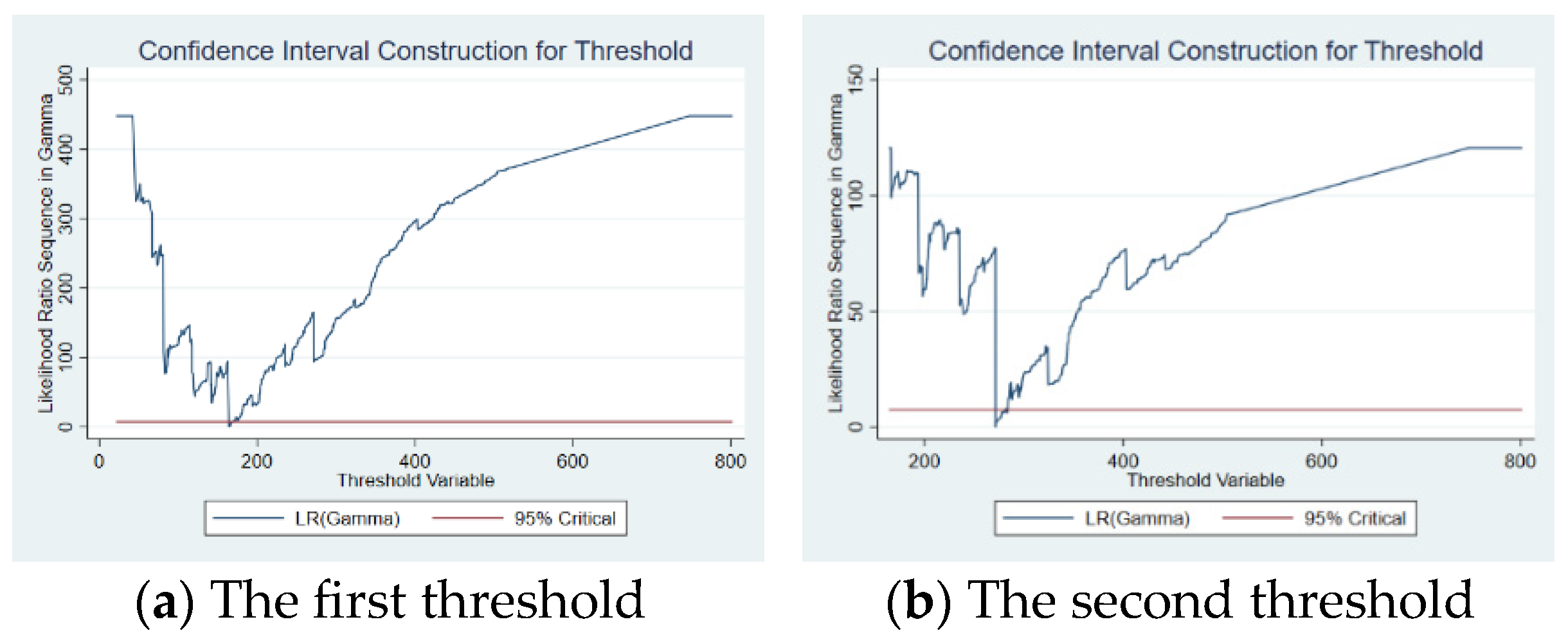
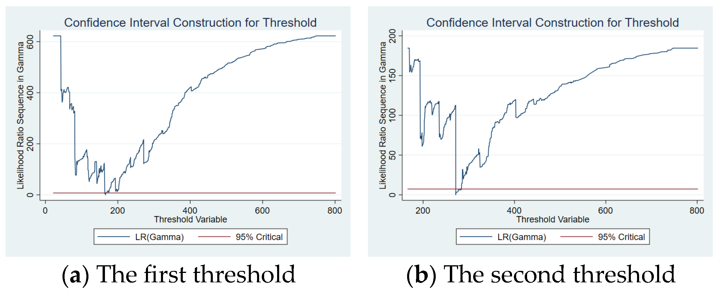
Second threshold	271.5	[271.5, 284.0]

presents the estimated threshold values. The first threshold is estimated at 164.1 km, with a 95% confidence interval ranging from 164.1 to 166.4 km. The second threshold is estimated at 271.5 km, with a 95% confidence interval between 271.5 and 284.0 km.

To further verify the robustness of these threshold estimates, we conducted sensitivity analyses regarding the model’s configurations. Specifically, we re-estimated the model under the assumption of heteroskedasticity and varied the trimming proportion for the grid search (ranging from 5% to 15%). The results indicate that the estimated threshold values remained highly consistent across these varying settings, confirming that threshold selection is robust and not driven by specific parameter constraints.

Figure 3 shows the likelihood ratio function plot for the second threshold estimation of inter-city distance. The lowest points of the LR statistics correspond to the true threshold values. Since both values in the figure fall below the critical value indicated by the horizontal line, the two thresholds are statistically significant and valid.

5.2. Descriptive Statistical Analysis: Talent Migration in the Yangtze River Delta

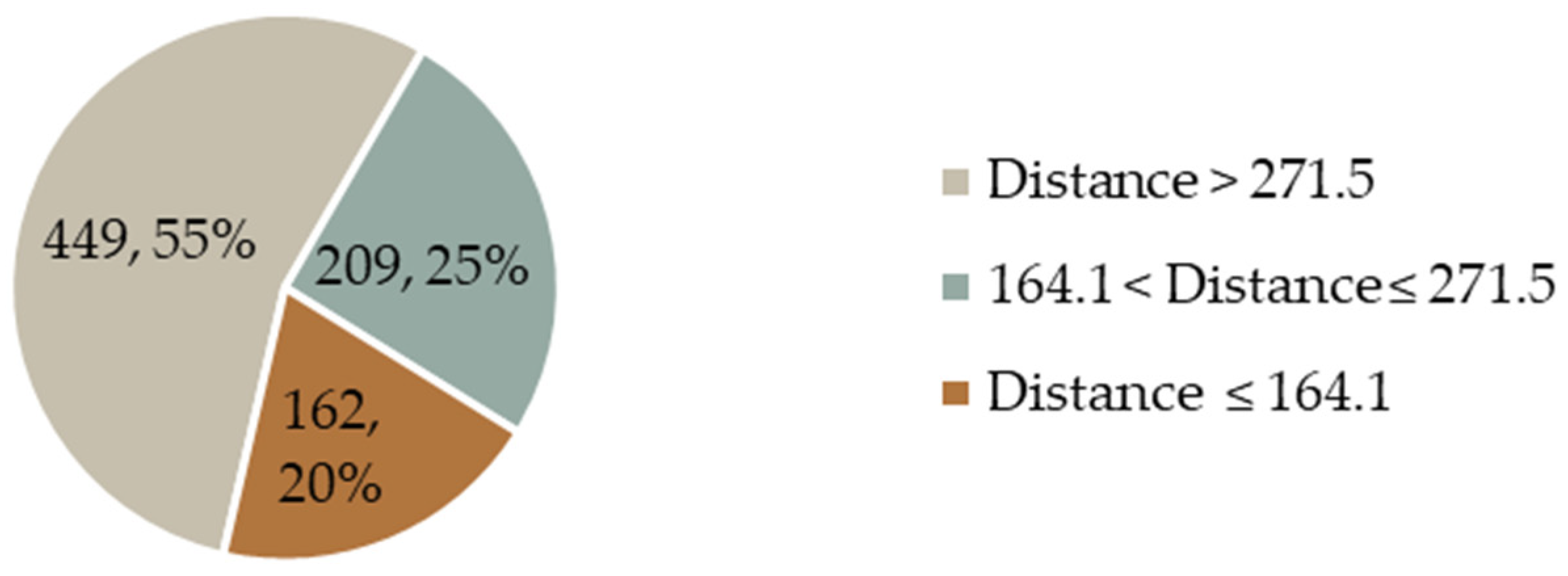
A total of 820 distinct inter-city distance records were obtained (excluding cases where the origin and destination cities are identical). Among these, 162 records exceed 164.1 km, 209 fall within the range of 164.1 km to 271.5 km, and 449 records are greater than 271.5 km, as illustrated in Figure 4.

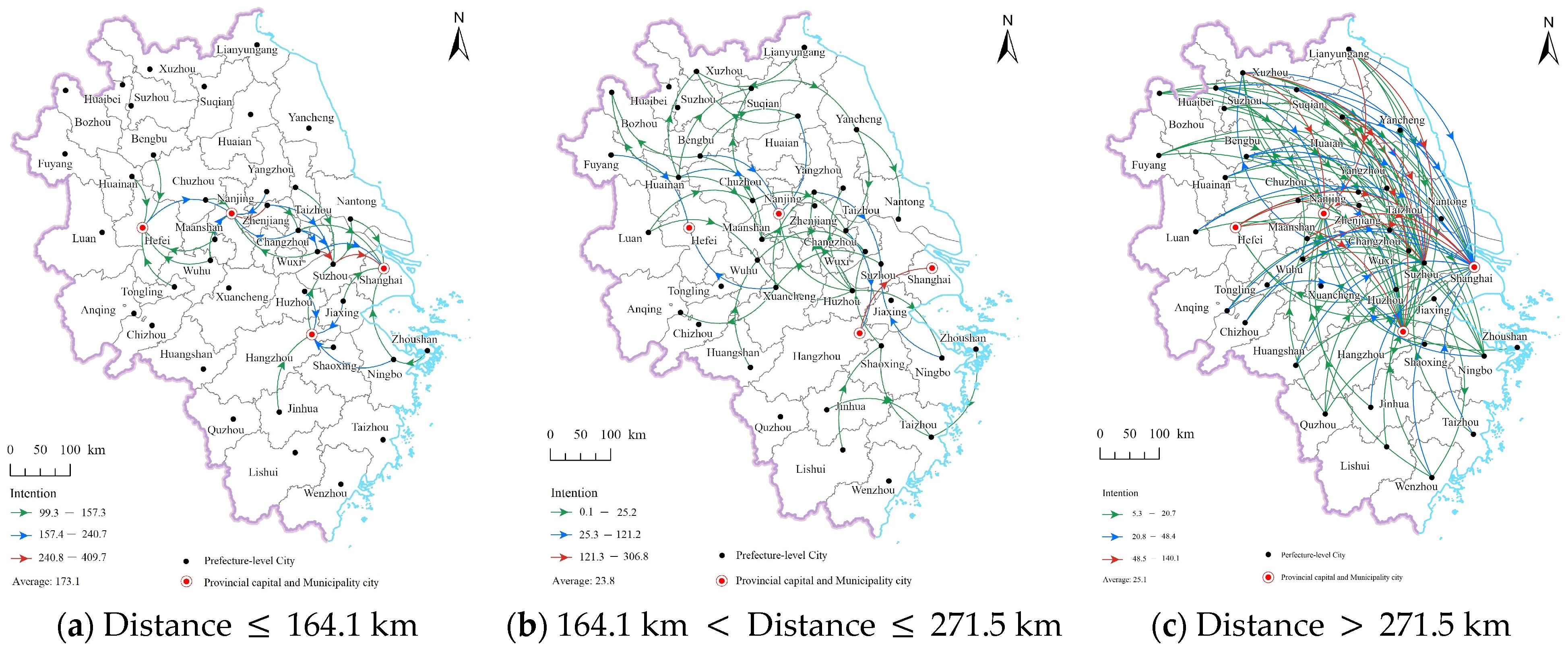
The top 20% of talent mobility flows across the three distance intervals are visualized in Figure 5. In the short-distance interval (≤164.1 km), 33 flows are identified, primarily concentrated between cities in southern Jiangsu and northern Zhejiang. Most of the economically developed cities in the Yangtze River Delta are located within this distance range. The medium-distance interval (164.1–271.5 km) contains 42 flows, mainly connecting northern Anhui, southern Jiangsu, and a few cities in Zhejiang. Unlike the other two intervals, destination cities in this range are not as distinctly concentrated. The long-distance interval (>271.5 km) comprises 90 flows. At these greater distances, talent tends to move from economically less developed cities to higher-tier economic centers such as Shanghai, Nanjing, Hangzhou, Suzhou, Wuxi, and Changzhou.

A comparison of talent mobility intention across the three intervals reveals distinct patterns. First, values in the short-distance interval range from 99.3 to 409.7, with a mean of 173.1, which is significantly higher than those in the other two intervals. This indicates a substantially stronger willingness to relocate over short distances. Second, the mean mobility intention in the long-distance interval (25.1) is slightly higher than that in the medium-distance interval (23.8). This suggests that mobility intention does not continuously decline with increasing distance; rather, it shows a slight rebound when moving from medium to long distances.

5.3. Economic Level and Talent Mobility Intention

After identifying the threshold values, the original sample was divided into three intervals for cross-sectional threshold regression: distances less than 164.1 km, distances between 164.1 km and 271.5 km, and distances greater than 271.5 km. The results are presented in

Table 8. Parameter results across distance intervals.

	Distance ≤ 164.1	164.1 < Distance ≤ 271.5	Distance > 271.5
Distance	−0.278 ***	−0.018	−0.011 ***
	(−3.56)	(−0.40)	(−4.85)
Ln_GDP	25.710 ***	3.329	2.735 ***
	(3.69)	(0.61)	(2.80)
Ln_Income	9.799	18.490	2.020
	(0.53)	(1.33)	(0.89)
Structure	3.912 ***	1.532 ***	0.602 ***
	(6.12)	(3.86)	(5.38)
Ln_ed	−0.005	0.041	0.007
	(−0.13)	(1.11)	(1.39)
Sn	10.560 **	6.147 **	4.715 ***
	(2.09)	(2.11)	(4.06)
Constant	−463.600 ***	−305.100 **	−69.910 ***
	(−3.11)	(−2.55)	(−4.02)

Note: * p < 10%, ** p < 5%, and *** p < 1%.

. It can be observed that the coefficients of economic level on talent mobility intention vary across these distance intervals, indicating the presence of a threshold effect and thus supporting Hypothesis 3. The nonlinear influence of economic level manifests specifically as follows:

1. When the distance is ‘short’ (distance ≤ 164.1 km), the coefficient of economic level on talent mobility is 25.710 (p < 0.01), indicating that a higher GDP in the destination city significantly boosts talent mobility intention. This reflects a strong economic driving effect on talent mobility.

On one hand, shorter distances reduce the need for individuals to relocate their families, allow them to retain most of their social networks and resources, and minimize adjustments to lifestyle and cultural habits, thereby lowering the overall cost of mobility. On the other hand, information is more transparent between nearby cities, making it easier for talent to perceive economic opportunities, such as higher salaries, industrial resources, and career development, which are offered by economically developed destinations. This transparency further strengthens mobility intention.

Under these conditions, the economic benefits gained from mobility significantly outweigh the costs, leading talent to prefer moving to economically strong cities within a short distance.

2. When the distance falls in the medium range (164.1 km < distance ≤ 271.5 km), the coefficient of economic level on talent mobility is 3.329 but statistically insignificant. This indicates structural failure of the economic driving mechanism, which can be attributed to two underlying causes.

First, regional industrial isomorphism limits the wage premium. Within the Yangtze River Delta, cities in this medium-distance range frequently share similar industrial structures. Unlike long-distance moves to top-tier financial centers that offer a substantial structural leap in income, relocating between functionally similar cities yields only limited marginal economic gains. The resulting wage gap is often insufficient to offset the associated migration costs, making talent less responsive to aggregate differences in economic size.

Second, a significant mismatch exists between the discontinuous jump in social costs and the prospective economic gains. This distance interval constitutes an awkward zone. It exceeds the practical radius for daily or weekly commuting, thereby disrupting the low-cost social maintenance possible in short-distance moves. Simultaneously, the destination cities lack the overwhelming economic agglomeration effects characteristic of super-metropolises. Faced with a sharp increase in the costs of social detachment and the absence of a compensating salary risk premium, the traditional pull exerted by economic volume alone becomes ineffective.

3. In the long-distance range (distance > 271.5 km), the coefficient of economic level on talent mobility is 2.735 (p < 0.01). Although the magnitude is smaller than in the short-distance range, it remains statistically significant. In this context, talent movement is driven by the high economic capacity of cross-regional hubs.

Although long distances typically involve inter-provincial or cross-regional mobility and entail higher costs, the agglomeration effects of destination cities become prominent, such as Shanghai and southern Jiangsu, as shown in Figure 5. The strong economic capacity compensates for these costs through notably higher salaries, access to scarce career opportunities, and other advantages, creating a strong attraction that motivates talent to overcome geographical barriers.

4. Compared to the short-distance range (≤164.1 km), the coefficient of economic level in the long-distance range (>271.5 km) is significantly smaller (2.735 vs. 25.710), indicating a weaker marginal effect on talent mobility. This may be attributed to the following reasons:

On one hand, the economic development levels of destination city clusters have already reached a certain threshold. As a result, talent may place greater emphasis on job compatibility and career development opportunities, thereby reducing the marginal effect of economic growth. On the other hand, higher mobility costs require that economic returns be substantial enough to offset these expenses. This effectively raises the threshold for mobility, limiting long-distance relocation to highly competitive or specialized talent who can obtain sufficient benefits from high-level economic centers to justify the costs. Such a screening effect restricts the scale of long-distance mobility, manifesting as a diminished marginal impact of economic level on talent movement.

5.4. Inter-City Distance and Talent Mobility Intention

As shown in Table 8, the estimated coefficients of distance on talent mobility intention vary significantly across different distance intervals, confirming the existence of a threshold effect and thus supporting Hypothesis 4. The nonlinear influence of inter-city distance manifests as follows:

1. When the inter-city distance is short (distance ≤ 164.1 km), the coefficient of distance on talent mobility intention is −0.278 (p < 0.01), indicating that for every additional kilometer of distance, talent mobility intention decreases by 0.278, demonstrating a strong negative effect. Within the transportation context of the Yangtze River Delta, distances within 164.1 km generally support high-frequency commuting, such as weekly or even same-day round trips. This enables talent to largely retain their original social resources and family support while maintaining lifestyle and cultural adaptability, yet still fully access the economic benefits offered by the destination city. Therefore, within this range, shorter distances strengthen talent mobility intention, whereas increased distance directly undermines this convenience, leading to a significant decline in willingness to move.

2. When the distance falls within the medium range (164.1 km < distance ≤ 271.5 km), its coefficient on talent mobility intention is −0.018 and statistically insignificant. This indicates that within this interval, the marginal deterrent effect of distance weakens.

This can be understood from two perspectives. First, within this range, commuting patterns for personal interaction have largely stabilized. The distance exceeds the threshold that permits weekly travel (approximately 164 km), causing the frequency of interaction to settle at a lower level, such as monthly or quarterly. Consequently, further increases in distance within this band generally do not lead to a substantial change in interaction frequency, rendering it statistically insignificant.

Second, when a journey already requires several hours, adding a few more kilometers of travel does not significantly alter its fundamental nature as a medium-to-long trip. The psychological impact of specific mileage differences on the decision-maker becomes minimal. As a result, mobility intentions in this context are influenced more by non-spatial factors—such as career opportunities, living environment, or family ties—while the weight of distance itself in the decision-making process diminishes.

3. When the inter-city distance is long (distance > 271.5 km), the coefficient of distance on talent mobility intention is −0.011 (p < 0.01), indicating that for every additional kilometer of distance, mobility intention decreases by only 0.011, demonstrating a weak negative effect. Within long-distance ranges, commuting frequency further declines (e.g., from monthly to quarterly). At this point, the marginal impact of increasing distance on commuting frequency stabilizes, while original social networks and family support are almost entirely disrupted. This ‘reset of social capital’ causes mobility decisions to rely more heavily on the economic benefits and personal development opportunities available in the destination city. As a result, the influence of distance gradually diminishes, manifesting as a relatively weak negative effect.

5.5. Endogeneity and Robustness Checks

To ensure the reliability and internal validity of the empirical findings, this section carries out a series of diagnostic tests. First, the two-stage least squares method with an instrumental variable is employed to address potential endogeneity concerns related to economic development. Second, we perform robustness checks by substituting geographic distance with temporal distance metrics to verify the persistence and stability of the threshold effects and by introducing additional controls for housing prices and cultural factors to address omitted variable bias.

5.5.1. Endogeneity Test

While regional economic development attracts talent, the influx of human capital may also drive local economic growth. To rigorously address this endogeneity and isolate the causal effect of economic factors on talent mobility, we employed a two-stage least squares approach using an instrumental variable approach. We constructed a spatially and temporally lagged instrument. Specifically, the IV is defined as the average GDP per capita of geographically adjacent cities over the five-year period from 2017 to 2021. Mathematically, for city $i$, the instrument $Z_i$ is calculated as follows:

$$Z_i={\displaystyle \frac{1}{N_k}}\sum _{k\in \mathcal{N}\left(i\right)}({\displaystyle \frac{1}{5}}\sum _{t=2017}^{2021}{GDP}_{k,t})$$

where $\mathcal{N}\left(i\right)$ denotes the set of cities that share a common border with city i. N_k is the number of cities in the set $\mathcal{N}\left(i\right)$.

The instrument satisfies both relevance and exclusion conditions. Its relevance is supported by strong regional economic agglomeration and spillover effects, which ensure that the historical economic performance of neighboring cities is closely correlated with the current economic level of the focal city. Meanwhile, the exclusion restriction is upheld because the five-year historical GDP data of neighboring cities are predetermined relative to the current period. It is theoretically implausible that past economic conditions in surrounding cities would directly influence an individual’s present migration decision toward the focal city, except through the channel of the focal city’s own contemporary economic development. The 2SLS estimation results are reported in

Table 9. Endogeneity test results (2SLS).

Variables	OLS	2SLS(IV)
Second-Stage Results:
Distance	−0.049 ***	−0.050 ***
	(−7.27)	(−7.83)
Ln_GDP	8.621 ***	14.504 **
	(3.69)	(2.18)
Ln_Income	5.621	−10.325
	(0.98)	(−0.68)
Structure	1.715 ***	1.933 ***
	(7.70)	(5.89)
Ln_ed	0.009	−0.008
	(0.67)	(−0.42)
Sn	7.770 ***	8.063 ***
	(3.84)	(4.25)
Constant	−198.602 ***	−80.279
	(−4.35)	(−0.78)
First-Stage Diagnostics:
IV		0.563 ***
		(16.30)
F-statistic		265.8

Note: * p < 10%, ** p < 5%, and *** p < 1%.

.

The first-stage results demonstrate a strong positive correlation between the instrument and the endogenous variable, with an F statistic of 265.8, well above the conventional threshold of 10, thereby rejecting the null hypothesis of weak instruments. After correcting for endogeneity in the second stage, the coefficient on GDP remains positive and statistically significant at 14.504 (p < 0.05). The qualitative consistency between the IV and baseline OLS estimates confirms the robustness of our main findings and indicates that they are not driven by reverse causality. Thus, the positive pull effect of economic development on talent mobility represents a causal relationship.

5.5.2. Robust Checks

1.

Replacing explanatory variable

To verify the robustness of our findings, we substituted geographic distance with temporal distance as the threshold variable. Specifically, we constructed two alternative metrics to capture travel costs:

(1) Rail commute time (RCT). This metric is defined as the minimum travel time between city pairs via direct train connections. Pairs without direct rail links were excluded, resulting in a restricted subsample of 642 observations. (2) Mixed commute time (MCT). To address the sample selection bias in the first method and maintain the full sample size (N = 1640), we supplemented the rail data with estimated travel times. For the 998 city pairs lacking direct rail connections, we estimated the commute time using the formula $\mathrm{T}\mathrm{i}\mathrm{m}\mathrm{e}=\mathrm{D}\mathrm{i}\mathrm{s}\mathrm{t}\mathrm{a}\mathrm{n}\mathrm{c}\mathrm{e}/100\mathrm{km}/\mathrm{h}$. These estimates were combined with the rail data to form a complete dataset. All temporal variables were measured in minutes and log-transformed prior to estimation.

Table 10. Results of thresholds for RCT and MCT.

	First Threshold		Second Threshold
	Value	95% Confidence Interval	Value	95% Confidence Interval
RCT (N = 642)	4.22 ***	[4.22, 4.22]	4.86 ***	[4.86,4.88]
MCT (N = 1640)	4.22 ***	[4.22, 4.26]	4.86 ***	[4.86,4.87]

Note: * p < 10%, ** p < 5%, and *** p < 1%.

presents the threshold estimation results using these temporal distance metrics. The results demonstrate remarkable consistency across both the subsample and the full sample.

Both models identify two highly significant thresholds at nearly identical values, with the first occurring at approximately 4.22 and corresponding to 68 min, and the second at 4.86 and corresponding to 130 min. This consistency implies that the boundary effect of distance on talent mobility is robust regardless of the sample size or the specific measurement of travel cost.

Figure 6 presents the likelihood ratio function graphs for threshold estimation. The horizontal red line in each graph represents the critical value at the 95% confidence level. The confidence intervals for both the RCT and the MCT are extremely narrow. This indicates that the threshold estimates are highly precise and statistically significant, further confirming that the structural break in the influence of distance is robust.

Table 11. Results of RCT and MCT estimation.

	Threshold Variable	RCT/MCT	t Value	Ln_GDP	t Value
RCT (N = 642)	RCT ≤ 4.22	−26.630 ***	−1.82	51.890 ***	2.97
	4.22< RCT ≤ 4.86	0.410	0.02	24.160 ***	3.56
	RCT > 4.86	−1.572 *	−1.84	6.676 ***	4.10
MCT (N = 1640)	MCT ≤4.22	−23.030 **	−2.35	33.740 ***	3.07
	4.22< MCT ≤4.86	−7.977	−0.92	13.140 ***	4.01
	MCT > 4.86	−1.324 **	−2.16	3.258 ***	4.73

Note: * p < 10%, ** p < 5% and *** p < 1%.

presents the estimation results where commuting time serves as both the threshold variable and a key explanatory variable. The results from both the RCT and MCT models are highly consistent, confirming the robustness of our findings. The estimated coefficients show that employing time distance as the threshold variable produces outcomes aligned with the geographic distance model, thereby confirming the robustness of the boundary effect.

2.

Controlling Omitted Variables

To mitigate potential omitted variable bias arising from the housing price gradient, innovation environment, and unobserved cultural factors, we re-estimated the model with three additional control variables.

First, we collected average housing price data for the 41 sample cities from 58.com (accessed on 1 January 2025), a leading real estate information platform in China, to control for the cost-of-living gradient. Second, we utilized the logarithm of the number of patent applications (Ln_zl) as a proxy for the regional innovation and entrepreneurship ecosystem. Third, to address the concern regarding regional culture and historical context, we introduced dialect distance as a proxy variable. We quantified the cultural distance between city pairs on a scale of 0 to 3, where a value of 0 indicates that the origin and destination belong to the same dialect point, representing the highest degree of cultural similarity, and a value of 3 indicates that they belong to completely different dialect super-groups, representing the lowest degree of cultural similarity. Given that dialect distance offers a more granular and precise measure of cultural proximity than administrative boundaries, we excluded the same-province dummy variable in this specification.

Table 12. Results of inter-city distance threshold effects.

Thresholds	Values	95% Confidence Interval
First threshold	166.2 ***	[164.1, 166.4]
Second threshold	271.5 ***	[271.5, 283.4]

Note: * p < 10%, ** p < 5% and *** p < 1%.

reports the threshold estimation results after adding these controls. The tests identify two distinct structural break points at 166.2 km and 271.5 km, both of which are statistically significant at the 1% level. These thresholds divide the spatial interaction into three regimes: a short-distance range (distance ≤ 166.2 km), a medium-distance range (166.2 km < distance ≤ 271.5 km), and a long-distance range (distance > 271.5 km). Notably, the first threshold (166.2 km) remains highly consistent with the baseline model.

Figure 7 displays the likelihood ratio (LR) function for the first and second threshold estimates. The horizontal red line represents the critical value at the 95% confidence level. The threshold parameters are identified where the LR statistic equals zero. As shown, the LR curves intersect the critical value line within narrow intervals, indicating that the confidence intervals are tight and that both threshold estimates are statistically significant and valid.

Table 13. Parameter results across distance intervals.

	Distance ≤ 166.2	166.2 < Distance ≤ 271.5	Distance > 271.5
Distance	−0.297 ***	−0.0547	−0.0189 ***
	(−3.98)	(−1.07)	(−5.66)
Ln_GDP	25.69 *	16.80 *	8.255 ***
	(1.92)	(1.82)	(7.21)
Ln_Income	−60.69 ***	−11.21	−8.593 ***
	(−3.64)	(−1.31)	(−4.40)
Structure	3.402 ***	1.520 ***	0.570 ***
	(6.12)	(3.49)	(6.45)
Ln_ed	−21.50 ***	−2.002	−1.838 ***
	(−3.30)	(−0.57)	(−2.61)
Ln_Hp	28.86 ***	18.20 ***	5.735 ***
	(2.78)	(3.86)	(4.46)
Dialect	−1.384	3.124 **	2.486 ***
	(−0.57)	(2.12)	(3.50)
Ln_zl	9.553	−7.882	−3.257 ***
	(0.90)	(−0.88)	(−3.28)
Constant	97.68	−158.6	−10.78
	(0.62)	(−1.30)	(−0.63)

Note: * p < 10%, ** p < 5% and *** p < 1%.

presents the parameter estimates across the three distance intervals. The results demonstrate strong robustness compared to the baseline model. Specifically, the coefficient of distance remains significantly negative in the short-distance regime (−0.297) and the long-distance regime (−0.019), confirming that the distance decay effect persists even after accounting for housing costs, cultural barriers, and innovation capacity.

Similarly, the coefficient of Ln_GDP maintains a consistent pattern with the baseline findings, exhibiting a strong positive driving effect in the short-distance regime (25.69) and a significant but diminished marginal effect in the long-distance regime (8.255). This confirms that the nonlinear mechanism of economic attraction remains robust.

5.6. Heterogeneity Analysis

Subsequent analysis further examines the threshold effects of inter-city distance from the perspectives of education level and age.

5.6.1. Education Level Heterogeneity

In the original sample, job seekers with bachelor’s degrees and those with postgraduate degrees were statistically analyzed separately, and a threshold test was conducted. The results are shown in

Table 14. Results of thresholds for educational level.

	First Threshold		Second Threshold
	Value	95% Confidence Interval	Value	95% Confidence Interval
Bachelor	142.7 ***	[121.0, 142.7]	271.5 ***	[271.5, 283.9]
Postgraduate	164.1 ***	[164.1, 166.4]	271.5 ***	[271.5, 282.7]

Note: * p < 10%, ** p < 5% and *** p < 1%.

. The difference between Table 14 and the previous analysis lies in the fact that the first threshold value for bachelor’s degree holders is 142.7, which is lower than that for postgraduate degree holders (164.1 km). This discrepancy may be attributed to the fact that bachelor’s degree holders, compared to postgraduates, have weaker capabilities in obtaining long-distance employment information and rely more on localized social networks. As a result, their mobility decisions are constrained by distance at an earlier stage.

Figure 8 presents the likelihood ratio function graphs for threshold estimation across different education levels. The lowest points of the LR statistics represent the true threshold values, all of which are below the critical values shown by the horizontal lines. This confirms that both thresholds are authentic and statistically valid.

Similarly, the different education levels were divided into distinct intervals based on the threshold values and estimated using OLS. To conserve space,

Table 15. Estimation results of different education level groups.

	Threshold Variable	Distance	t Value	Ln_GDP	t Value
Bachelor	Distance ≤ 142.7	−0.305 ***	−4.02	33.850 ***	6.55
	142.7 < Distance ≤ 271.5	−0.038 *	−1.65	16.020 ***	7.76
	Distance > 271.5	−0.005 ***	−3.27	6.008 ***	9.31
Postgraduate	Distance ≤ 164.1	−0.038	−1.46	10.74 ***	5.83
	164.1 < Distance ≤ 271.5	0.006	0.30	5.265 ***	4.21
	Distance > 271.5	−0.002 ***	−3.20	2.008 ***	2.52

Note: * p < 10%, ** p < 5% and *** p < 1%.

only reports the estimation results for inter-city distance and economic level. Table 15 shows that for postgraduates in the first interval (≤164.1 km), the impact of economic level on mobility intention is positive and significant (10.74), but the coefficient is considerably smaller than that of bachelor’s degree holders (33.85).

This difference suggests that while postgraduates are attracted to economically developed cities, their sensitivity to aggregate economic volume is lower than that of undergraduates. The reason may lie in the high degree of specialization in research fields and career paths among postgraduates. When making mobility decisions, they typically consider not only a destination’s economic capacity but also their own career development platforms. For example, doctoral graduates often prioritize institutional platform levels, such as employment at ‘Double First-Class’ universities or top-tier research institutions, over purely economic volume. Consequently, the marginal utility of destination GDP is somewhat diluted by these non-economic professional requirements, resulting in a weaker economic driving effect compared to bachelor’s degree holders who are more responsive to general labor market opportunities provided by high-GDP cities.

5.6.2. Age Heterogeneity

Based on the original sample, job seekers aged 30 and below and those above 30 were analyzed separately, with threshold tests conducted accordingly. The results are presented in

Table 16. Results of thresholds for different ages.

	First Threshold		Second Threshold
	Value	95% Confidence Interval	Value	95% Confidence Interval
30 and below	166.2 ***	[164.1, 176.9]	271.5 ***	[271.5, 284.0]
Above 30	121.0 ***	[121.0, 121.0]	164.1 ***	[164.1, 164.7]

Note: * p < 10%, ** p < 5% and *** p < 1%.

.

In the subgroup above 30 years old, the first and second threshold values of city distance are 121 and 164.1 km, respectively, both lower than those in the full sample. This may be attributed to the following reasons.

Job seekers above 30 typically bear greater family responsibilities, including a spouse’s employment, children’s education, and care for elderly parents. Shorter distances facilitate more frequent commuting, which helps mitigate the practical and psychological costs of relocation. Consequently, this demographic exhibits greater sensitivity to distance. Moreover, individuals above 30 are often in the mid-career stage, having accumulated considerable professional experience, industry-specific resources, and localized social networks. Longer distances make it more difficult to leverage these existing career-specific assets, leading to significantly higher opportunity costs compared to those under 30. Hence, the threshold values for distance are lower in this group.

Figure 9 shows the likelihood ratio function plots for threshold estimation across different ages. The lowest points of the LR statistics correspond to the true threshold values. Since all these points fall below the critical values indicated by the horizontal lines, both thresholds are statistically significant.

Table 17. Threshold estimate results for different age groups.

	Threshold Variable	Distance	t Value	Ln_GDP	t Value
30 and below	Distance ≤ 166.2	−0.172 ***	−3.14	35.22 ***	7.91
	166.2 < Distance ≤ 271.5	−0.007	−0.15	16.73 ***	6.01
	Distance > 271.5	−0.006 ***	−3.25	7.030 ***	8.99
Above 30	Distance ≤ 121	−0.151 ***	−3.01	8.759 ***	3.13
	121 < Distance ≤ 164.1	0.092	1.57	4.502 ***	3.66
	Distance > 164.1	−0.002 ***	−5.08	1.465 ***	7.54

Note: * p < 10%, ** p < 5% and *** p < 1%.

reports the estimated effects of inter-city distance and economic level on talent mobility intention across different distance intervals.

Regarding distance, the threshold of the older group (121 km) is notably lower than that of the younger group (166.2 km), confirming that the spatial range of mobility for individuals above 30 is more restricted.

Furthermore, a distinct reversal is observed in the economic dimension compared to the distance effect. The coefficients for economic level are significantly larger in the younger subgroup compared to the older one (e.g., 35.22 vs. 8.759 in the short-distance range), suggesting that younger job seekers are much more responsive to destination economic capacity. This may be attributed to the fact that younger individuals are in the career accumulation phase and are highly sensitive to the “thick labor market” effects provided by high-GDP cities, actively seeking regions with maximum growth potential. In contrast, those above 30 face higher migration costs and “mooring effects” due to family responsibilities (e.g., children’s education, spousal employment) and established social networks. These factors increase the threshold for relocation, making them less likely to move solely based on the macro-economic level of a destination. Consequently, their mobility intention exhibits lower elasticity to economic development compared to the younger demographic.

5.6.3. Sectoral Heterogeneity

We conduct threshold regression comparisons by selecting two distinct groups from the sample: knowledge-intensive industries (KIs) and labor-intensive industries (LIs). In accordance with the National Economic Industry Classification and Codes, knowledge-intensive industries include Information Transmission, Software, and Information Technology Services (industry codes: J1–J3); Financial Intermediation (J4–J7); Scientific Research and Technical Services (M1–M3); and Business Services (L2). Labor-intensive industries comprise Manufacturing (C1–C31); Construction (E1–E4); Wholesale and Retail Trade (F1–F2); and Accommodation and Catering Services (H1–H2).

Table 18. Results of thresholds for different sectors.

	First Threshold		Second Threshold
	Value	95% Confidence Interval	Value	95% Confidence Interval
KI	164.1 ***	[164.1, 166.2]	271.5 ***	[271.5, 280.0]
LI	121.0 ***	[121.0, 121.0]	166.2 ***	[164.1, 277.2]

Note: * p < 10%, ** p < 5% and *** p < 1%.

reports the results of the threshold tests and the estimated threshold values for the distance variable. The double-threshold model shows statistical significance at the 1% level for both industry types. For knowledge-intensive industries, the two threshold values are estimated at 164.1 and 271.5. In contrast, the threshold values for labor-intensive industries are significantly lower, at 121.0 and 166.2. Notably, the first threshold for knowledge-intensive industries (164.1 km) almost coincides with the second threshold for labor-intensive industries (166.2 km). This indicates that talent mobility in labor-intensive industries is more sensitive to distance, whereas talent in knowledge-intensive industries exhibits a broader spatial tolerance.

Figure 10 shows the likelihood ratio function plots for threshold estimation across different industries. The lowest points of the LR statistics correspond to the true threshold values. Since all these points fall below the critical values indicated by the horizontal lines, both thresholds are statistically significant.

Table 19. Threshold estimate results for different sectors.

	Threshold Variable	Distance	t Value	Ln_GDP	t Value
KI	Distance ≤ 164.1	−0.037 ***	−3.22	3.367 ***	6.59
	164.1 < Distance ≤ 271.5	0.001	0.09	1.497 ***	4.71
	Distance > 271.5	−0.001 ***	−4.35	0.523 ***	8.91
LI	Distance ≤ 121	−0.207 ***	−3.21	15.07 ***	5.45
	121 < Distance ≤ 166.2	0.078	1.14	5.745 ***	5.60
	Distance > 166.2	−0.005 ***	−6.39	2.131 ***	9.86

Note: * p < 10%, ** p < 5% and *** p < 1%.

presents the estimation results for the regime-dependent coefficients, illustrating how the impact of distance and economic scale varies across the identified intervals.

Notably, the coefficients for distance in the labor-intensive (LI) sector are significantly larger in absolute magnitude than those in the knowledge-intensive (KI) sector (e.g., −0.207 vs. −0.037 in the first regime), indicating higher sensitivity to distance among labor-intensive industries. That is, as distance increases, the strength of economic linkage declines more rapidly in the LI group, which is consistent with their lower threshold values discussed earlier. Furthermore, the coefficients for Ln_GDP are consistently larger in the LI sector compared to the KI sector across all regimes, suggesting that labor-intensive industries are more responsive to changes in regional economic size. This may be attributed to the characteristics of labor-intensive products, which typically rely on mass market consumption and scale effects, making the sheer economic volume of a region a stronger motivator for interaction.

5.6.4. City Economic Hierarchy Heterogeneity

Given the significant differences in resource agglomeration capacity and spatial reach among cities at different economic levels, the sample was divided into two groups: Trillion-CNY GDP cities (TC), which include Shanghai, Nanjing, Hangzhou, Hefei, Suzhou, Ningbo, Wuxi, Changzhou, and Nantong, and Non-trillion-CNY GDP cities (NTC), comprising the remaining cities among the 41 studied. The corresponding threshold estimation results are presented in

Table 20. Results of thresholds for different economic hierarchies.

	First Threshold		Second Threshold
	Value	95% Confidence Interval	Value	95% Confidence Interval
TC	193.8 ***	[82.7, 203.4]	—	—
NTC	94.4 ***	[94.4, 100.9]	271.5 ***	[271.5, 282.7]

Note: * p < 10%, ** p < 5% and *** p < 1%.

.

As shown in Table 20, the TC group has a single distance threshold of 193.8 km, whereas the NTC group has two thresholds, at 94.4 km and 271.5 km. First, the fact that only one threshold was identified for the TC group may be attributed to its relatively small sample size (N = 360), which could make it difficult to detect a second threshold. Second, the first threshold of the NTC group (94.4 km) is much smaller than that of the TC group (193.8 km), indicating that cities with smaller economic scale have a shorter effective range for attracting talent.

Figure 11 shows the likelihood ratio function plots for threshold estimation across cities with different GDP values. The lowest points of the LR statistics correspond to the true threshold values. Since all these points fall below the critical values indicated by the horizontal lines, both thresholds are statistically significant.

Table 21. Threshold estimate results for different economic hierarchies.

	Threshold Variable	Distance	t Value	Ln_GDP	t Value
TC	Distance ≤ 193.8	−0.54 ***	−2.64	100.40	1.32
	Distance > 193.8	−0.08 ***	−4.00	19.19	0.84
NTC	Distance ≤ 94.4	−0.79 **	−2.59	19.62	1.19
	94.4 < Distance ≤ 271.5	−0.08 ***	−3.19	9.41 **	2.24
	Distance > 271.5	−0.01 ***	−4.85	2.74 ***	2.80

Note: * p < 10%, ** p < 5% and *** p < 1%.

illustrates how distance acts as a friction factor preventing talent flow. In the first regime, the negative coefficient for the NTC group (−0.79) is larger in magnitude than that of the TC group (−0.54). This implies that talent mobility towards smaller cities is highly sensitive to commuting or migration costs; a slight increase in distance significantly deters inflow. Conversely, the high expected returns, e.g., higher wages, and better career prospects in the TC group help offset the friction of distance, making talent less sensitive to geographical barriers. Notably, the economic level is not significant in the TC group. This may be because, for cities in the TC group, the attraction effect of GDP has likely reached saturation, meaning that further GDP growth does not significantly enhance their ability to attract more talent.

6. Conclusions and Policy Implications

6.1. Conclusions and Discussion

This study takes the 41 cities within the Yangtze River Delta as its research sample to empirically examine the impact of inter-city distance on talent mobility intentions. The main findings are as follows:

1. Inter-city distance exerts a significant negative impact on talent mobility intention. This finding is consistent with those of numerous previous studies, such as Molloy, Smith, and Wozniak [17] in the context of employment and Van der Wouden and Youn [16] regarding learning collaboration. In this paper, it is argued that the underlying mechanisms primarily operate through talent’s attachment to specific places, such as their birthplace, place of education, or family location, the costs associated with the loss of interpersonal and social networks, and potential challenges related to adapting to different cultural practices and lifestyle habits.

2. Inter-city distance plays a negative moderating role between talent mobility intention and economic level. The essential goal of talent migration is to maximize the return on human capital. As distance increases, the costs associated with migration will inevitably rise. With the same level of economic attractiveness, the farther the distance between cities, the lower the willingness of talents to move. A study by Shi, Geng, Huang, Mao, and Jia [21] found a nonlinear relationship between urban factors and migration, which is consistent with the conclusion of this study. The difference is that this study focuses more on distance rather than on the nonlinear effect of multiple factors.

3. The effect of a destination’s economic level on talent mobility intention is characterized by a threshold effect contingent upon inter-city distance. These nonlinear results corroborate the complexity of the push–pull and spatial interaction theories. Our findings suggest that the trade-off between migration costs (friction) and economic benefits (pull) is not constant but varies structurally across spatial scales. Specifically, this effect manifests as a strong economic driver at short distances, an offsetting effect at medium distances, and a potential economic attraction effect at long distances. Empirically, short-distance flows (<164.1 km) exhibit the highest intensity, whereas medium-distance flows prove least attractive. In contrast, long-distance flows (>271.5 km) experience a slight rebound as talent selectively targets major economic hubs. Similarly, a threshold effect is observed between inter-city distance and talent mobility intention. While Na and Liu [22] measured urban attractiveness using distance decay patterns without specifying concrete distance thresholds, this study employs a threshold model to identify explicit distance thresholds of 164.1 km and 271.5 km, thereby offering a more structured understanding of how distance shapes mobility patterns across different ranges.

From the perspective of regional sustainability, identifying these thresholds is crucial. It provides a scientific basis for optimizing the spatial structure of urban agglomerations, suggesting that effective management of these “mobility zones” can reduce spatial mismatch and foster a more integrated and resilient regional talent ecosystem.

4. Heterogeneity analysis reveals that sensitivity to distance varies significantly across individual and urban characteristics. Regarding individual attributes, bachelor’s degree holders exhibit a smaller first threshold value, which may be attributed to their relatively limited information acquisition capabilities compared to postgraduates. Similarly, job seekers aged 30 and above show significantly smaller threshold values and higher sensitivity to distance than younger groups, likely due to heavier family responsibilities and higher opportunity costs. Regarding sectoral differences, talent in labor-intensive industries exhibits significantly lower thresholds (121.0 km) compared to in knowledge-intensive industries (164.1 km). This indicates that talent in traditional sectors is more constrained by distance, whereas knowledge workers possess broader spatial tolerance. Regarding city economic hierarchy, Trillion-CNY GDP cities demonstrate a much larger effective attraction radius (193.8 km) than Non-trillion-CNY cities (94.4 km). This implies that the high expected returns and career platforms in top-tier cities can effectively offset distance friction, whereas smaller cities primarily rely on localized talent pools within a narrower range.

Recognizing these disparities is vital for social sustainability. It underscores the need for differentiated policies that support vulnerable groups (e.g., older workers or those in traditional sectors) and smaller cities, thereby promoting a more inclusive and balanced urbanization process.

6.2. Policy Implications

Based on the above findings, the following policy recommendations are proposed to enhance talent mobility in the Yangtze River Delta:

1. Construct a tiered regional talent policy framework considering city economic hierarchy. Trillion-CNY GDP cities, with their strong long-distance attraction, should act as regional hubs. They need to establish “Talent Enclaves” and remote R&D centers in peripheral areas to extend their resource radiation. Conversely, Non-trillion-CNY cities, which have a smaller attraction radius, should focus on localized retention. Specific measures include aligning local industrial chains with neighboring core cities to avoid homogeneous competition and introducing high-speed rail monthly passes to facilitate short-distance commuting and dual-city living.

2. Strengthen compensation mechanisms for migration costs. To address the market failure in medium-distance mobility, we recommend establishing a talent mobility risk fund co-financed by governments and enterprises. This fund would provide specific financial support, including one-time settling-in allowances and rental subsidies for talent relocating beyond a certain distance. Furthermore, the fund could cover potential risks such as compensation for probation period failure and transportation subsidies for inter-city job interviews. These concrete measures help alleviate decision-making concerns by sharing the economic risks associated with relocation.

3. Implement precisely tailored policies based on individual and sectoral heterogeneity. For labor-intensive industries, which are highly sensitive to distance, governments should organize collaborative recruitment fairs within a specific radius and provide inter-city shuttle bus services for industrial parks to solve commuting difficulties. For knowledge-intensive industries, policies should encourage cross-regional project cooperation to utilize their higher spatial tolerance. Regarding demographic groups, digital job information networks should be built for bachelor’s degree holders to bridge information gaps. For mid-career talent, family support measures such as reserved inter-city school placements for children and instant cross-region medical insurance settlements are crucial to reducing the opportunity costs of migration.

6.3. Limitations and Future Research

Finally, some limitations of this study should be acknowledged to provide context for the findings and direction for future work.

First, a primary limitation concerns the dependent variable. This study relies on talent mobility intention rather than actual migration behavior. While mobility intention is widely recognized as a significant predictor of future migration, it does not strictly equate to the final realization of relocation. The gap between intention and behavior may vary across distance intervals. This is particularly relevant in the medium-distance zone identified in this study. In this interval, where the “pull” of economic incentives and the “push” of migration costs largely offset each other, the decision-making process becomes more complex and volatile. Consequently, the conversion rate from intention to actual behavior in this “hesitation zone” might be lower or more susceptible to external shocks compared to short- or long-distance flows.

Second, the generalizability of these findings is limited by the unique characteristics of the Yangtze River Delta region. This area represents a highly developed context within China, featuring the nation’s most dense high-speed rail network and advanced economic integration. Therefore, the precise distance thresholds identified in this study may not apply directly to less developed regions, even though the fundamental nonlinear mechanisms are likely still applicable.

Third, the analysis concentrates on internal regional integration dynamics and does not comprehensively address the interactive relationships between the Yangtze River Delta and other major economic hubs. In practice, talent flows operate within a multipolar competitive environment that includes regions such as the Pearl River Delta and the Beijing–Tianjin–Hebei area, a dimension beyond the focus of our current intra-regional framework.

To address these constraints, subsequent research should advance in several key areas. Future studies could incorporate actual migration records to quantitatively examine the discrepancy between mobility intention and real behavior, with particular attention paid to testing the proposition of greater instability within the medium-distance range.

Further exploration is also needed to identify the specific factors contributing to the insignificant effects observed at intermediate distances, which would elucidate decision-making processes in this transitional zone.

Comparative analyses conducted in other economic zones would assist in evaluating the broader relevance of these spatial principles and in calibrating threshold parameters according to varying developmental contexts. Finally, upcoming models should integrate inter-regional interaction components to better represent the complexities of talent distribution and competition at a national scale.