Fine Identification of Lake Water Bodies and Near-Water Land Using Multi-Source Remote Sensing Fusion: A Case Study of Weishan Lake, China

Abstract

Lakes play a crucial role in maintaining agricultural irrigation water sources, regulating climate, and supporting the long-term resilience of regional ecosystems. However, accurately delineating the boundaries between lakes and land remains challenging due to seasonal hydrological fluctuations, spectral obfuscation with farmland, and the limitations of single-sensor methods. This study constructs a multi-source remote sensing framework integrating Sentinel-1 SAR, Sentinel-2 optical data, DEM, and key environmental variables to identify the water body, near-water body, and non-water surface of Weishan Lake, a major irrigation source in northern China. The study systematically compares various methods, including the optical index method, SAR-based threshold segmentation, and machine learning classifiers. The results show that the random forest model has higher accuracy and temporal robustness. Introducing the “near-water body” category allows for more accurate characterization of transitional areas sensitive to seasonal hydrological and agricultural processes. Migration tests of the model in three external lake systems demonstrate its strong generalization ability, while correlation analysis and SHAP-based analysis indicate that NDVI and elevation are the main factors influencing the spatial pattern of water and land. The proposed framework supports sustainable irrigation management by enabling accurate water boundary monitoring and enhancing the understanding of agricultural hydrological interactions.

1. Introduction

Lakes and their surrounding landscapes play a critical role in maintaining regional hydrological stability, sustaining agricultural irrigation, and supporting long-term socio-ecological resilience. With the intensification of human activities and the expansion of irrigated cropland, lake water bodies increasingly exhibit marked spatial fluctuations and pronounced seasonal dynamics. Accurately capturing these changes is essential for ensuring the sustainable allocation of freshwater resources, improving irrigation scheduling, and mitigating the risks posed by climate variability. Under combined pressures from climate change and anthropogenic disturbance, the temporal evolution of lake surface extent and its spatial configuration have emerged as a pressing challenge for ecosystem service maintenance and sustainable regional development. Remote sensing, with its advantages of multi-temporal, long-term, and large-scale observation, has become a key tool for revealing and quantifying such spatiotemporal changes [1,2]. The advancement of medium- and high-resolution optical imagery and synthetic aperture radar (SAR) data has particularly facilitated dynamic monitoring of water bodies across various spatial scales—from local to regional [3,4]. However, spectral confusion between water and other surface features such as shadows, shallow zones, and riparian vegetation, coupled with seasonal water level variations and imaging inconsistencies, poses severe challenges to high-accuracy water extraction [5]. Therefore, integrating multi-source remote sensing data and method optimization for regional-scale water extraction and time-series analysis holds both theoretical and practical importance.

Existing research can be broadly categorized along two dimensions: methodological development and empirical application. In optical remote sensing, indices such as the NDWI and NDVI have been widely applied for wetland dynamics monitoring and ecological assessment [6,7]. However, their performance is often limited by water turbidity, floating debris, and shadow effects, and threshold values must be dynamically adjusted across sensors and time periods. To address these limitations, methods combining Otsu optimization, adaptive thresholding, and Canny edge detection have been proposed to enhance boundary delineation accuracy [8,9]. SAR data, with its all-weather and day–night imaging capability, shows significant advantages for water detection and flood monitoring under cloudy or rainy conditions. Studies based on Sentinel-1 VV/VH polarization data have incorporated temporal and textural features to improve the stability of inundation extraction [10,11]. Nevertheless, SAR images remain sensitive to terrain, vegetation, and backscattering characteristics, leading to potential misclassification. To mitigate these issues, researchers have integrated optical, DEM, and statistical features for fusion-based correction [12,13]. Furthermore, recent thresholding improvements combine the Otsu algorithm with edge detection or index variance metrics (e.g., MAWEI) to enhance temporal consistency in water boundary identification [8,9].

Machine learning and deep learning approaches have also been extensively adopted for water extraction. From traditional classifiers such as Random Forest (RF), Support Vector Machine (SVM), and Classification and Regression Tree (CART) to convolutional neural network (CNN)-based semantic segmentation models (e.g., WBE-NN), studies have demonstrated the superior performance of deep learning in complex environments and small water body recognition. However, these models are highly sensitive to sample quality, sensor consistency, and generalization capability [14,15]. For small or near-shore water bodies, recent studies have developed domain-knowledge-based multi-source fusion networks and weakly supervised learning strategies to improve recognition accuracy and cross-domain adaptability [16,17]. In addition, semantic segmentation of high-resolution imagery, multi-scale feature enhancement, and object-based image analysis (OBIA) have been shown to improve boundary detection and class consistency in complex environments [18,19,20].

At the empirical level, existing studies span from small watersheds to large basins, including flood mapping based on PlanetScope imagery and the retrieval of water bodies and suspended sediments using Landsat time-series data and the GEE platform [21,22]. However, most studies remain limited to single-method or site-specific experiments and lack systematic comparisons of multi-source data (optical + SAR + DEM), temporal stability assessments in near-shore zones, and evaluations of model transferability across seasons, sensors, and terrain conditions [4].

In terms of driving factors, the spatiotemporal dynamics of water bodies are influenced by the complex interactions of natural and anthropogenic factors. Key environmental drivers such as climate variability (e.g., precipitation patterns and temperature fluctuations) and human activities (e.g., agricultural irrigation, water diversion, and land use change) significantly alter hydrological conditions and surface water extent [4]. These changes are often nonlinear, making them difficult to detect and quantify. Remote sensing techniques, including spectral indices such as the Normalized Difference Water Index (NDWI) and advanced machine learning algorithms, have proven effective in capturing such dynamic changes [6]. However, spectral confusion between water bodies and land cover such as vegetated wetlands, shaded areas, and moist soils often leads to classification uncertainty, especially in transitional zones [6]. Understanding these influencing factors and their interactions is crucial for developing robust water intake approaches and sustainable water resource management strategies.

In summary, this study focuses on Weishan Lake and its surrounding area in Shandong Province, integrating multi-temporal Sentinel-1 SAR and Sentinel-2 optical imagery with SRTM/DEM data. It combines index-based, SAR threshold optimization, and machine learning approaches with domain-knowledge-guided data fusion strategies.

Through quantitative accuracy assessment and error analysis, this study aims to advance the practical applicability of multi-source remote sensing for agricultural water monitoring. Unlike previous studies that primarily focus on binary water–land classification, this research introduces an explicit near water land category to represent transitional zones between open water and surrounding croplands, thereby improving boundary characterization in complex agro-hydrological environments.

Specifically, the objectives are to: (1) systematically compare optical index methods, SAR-based thresholding (VV/VH ratio with adaptive thresholds), and machine learning approaches (RF and CART), with particular attention to their stability and misclassification behavior in near-water areas; (2) construct multi-seasonal water frequency maps and change detection results within a unified Google Earth Engine framework to enhance reproducibility and scalability; and (3) evaluate model transferability and temporal adaptability across shoreline buffers and small water bodies, and assess the added value of multi-source data fusion for fine-scale water extraction.

By integrating a tri-class classification scheme, multi-seasonal modeling, and cross-regional validation, this study provides new methodological insights into refined water–land boundary mapping. The proposed framework supports improved estimation of irrigation lake water availability and offers practical implications for data-driven agricultural water governance and sustainable resource management.

2. Materials and Methods

2.1. Study Area and Data Sources

2.1.1. Study Area

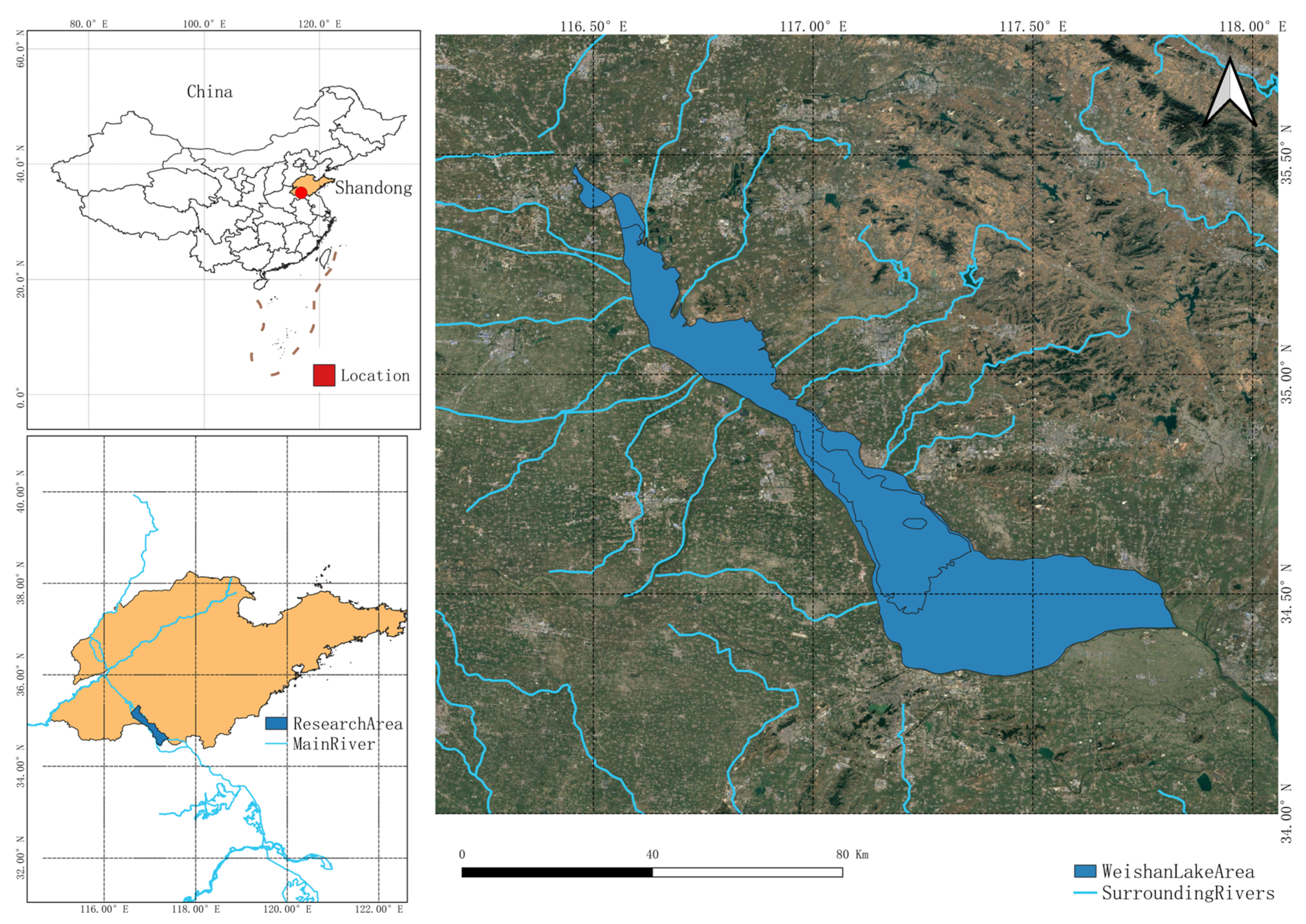
Weishan Lake, one of the largest freshwater lakes in northern China and a key component of the eastern route of the South-to-North Water Diversion Project, provides a model case for water resource monitoring research oriented towards sustainable development. Besides its ecological value, Weishan Lake is also an important irrigation water source, supporting widespread agricultural production in the surrounding area. The region has a complex hydrological pattern, encompassing open water areas, riparian wetlands, irrigation canals, and paddy fields, all of which are highly sensitive to seasonal water level changes. The lake’s irregular shoreline and the dynamic interactions between open water areas, wetlands, and cultivated land introduce significant uncertainties to the delineation of water body boundaries using traditional remote sensing techniques. Therefore, Weishan Lake provides an ideal location for advancing fine-scale classification of irrigation-related water bodies and transitional zones in near-water agriculture. For an overview and geographical location of the study area, please refer to Figure 1.

2.1.2. Multi-Source Remote Sensing Data

This study integrates optical, radar, topographic, and environmental datasets to construct a multi-source remote sensing framework for the refined extraction of water and near-water bodies. Sentinel-2 Multispectral Instrument (MSI) imagery and Sentinel-1 Synthetic Aperture Radar (SAR) data were jointly employed to capture complementary information on spectral reflectance and surface backscatter characteristics. The Shuttle Radar Topography Mission (SRTM) Digital Elevation Model (DEM) provided terrain elevation and slope information, both of which are essential in characterizing hydrological gradients and topographic constraints that influence the spatial distribution of water bodies [23].

To further account for hydrometeorological variability and surface energy exchange processes, additional environmental variables were introduced. The ERA5-Land reanalysis dataset was used to obtain near-surface air temperature and total precipitation, representing key climatic controls on lake hydrology. Meanwhile, the FAO WaPOR (Level 1 Actual Evapotranspiration) product was incorporated to quantify evapotranspiration intensity, which serves as an important indicator of water loss and agricultural irrigation demand in the surrounding plain area. These datasets were selected for their high temporal consistency, reliable global coverage, and compatibility with Sentinel data in spatial resolution after resampling. For details on the data and its uses, please refer to

Table 1. Remote sensing data sources used in this study.

Data Source	Bands/Information	Spatial Resolution	Main Application
Sentinel-1	VV polarization VH polarization	10 m	Use thresholding to extract water bodies and analyze surface scattering characteristics.
Sentinel-2	Visible light bands	10 m	Calculate water indices such as NDWI/MNDWI and classify land cover.
	Near-infrared band	10 m
SRTM DEM	Elevation data	20 m	Provide terrain constraints to assist in classification and subsequent accuracy improvement.
ERA5-Land	Temperature (2 m)	0.1° (~9 km)	Surface temperature and rainfall as climatic drivers
	Precipitation (total)
FAO WaPOR L1_AETI_D	Actual Evapotranspiration (AET)	250 m	Estimation of surface water and moisture loss relevant to irrigation demand

.

All datasets were temporally harmonized and spatially aligned to a uniform coordinate reference system (EPSG:4326). The ERA5-Land and WaPOR datasets were averaged to represent annual mean conditions, while Sentinel-based optical and radar data were resampled to a spatial resolution of 10 m to ensure consistency with classification inputs. Each dataset was clipped to the buffered research area of Weishan Lake to minimize computational redundancy.

Furthermore, a vegetation index (NDVI) was derived from Sentinel-2 imagery to quantify vegetation coverage and phenological variation within the study region. This index was not treated as a separate dataset but was computed directly from the Sentinel-2 surface reflectance bands (B8 and B4). The NDVI provides an effective proxy for vegetation-water interactions, thereby enhancing the explanatory power of subsequent correlation and factor analyses [24].

The integration of these diverse datasets ensures a robust and transferable foundation for multi-temporal water classification and environmental interpretation. By combining dynamic surface observations with atmospheric and land surface drivers, this study establishes a comprehensive multi-source data framework suitable for both classification and subsequent impact factor analysis.

2.2. Water Body Extraction and Accuracy Assessment

To address the challenges of boundary ambiguity and methodological adaptability in water body identification, this study developed an integrated multi-source and multi-algorithm extraction framework. First, the conventional Normalized Difference Water Index (NDWI) method was employed to perform static identification of typical water bodies and to obtain high-confidence water boundaries. Second, Sentinel-1 SAR data were incorporated, and the Otsu adaptive thresholding method based on VV/VH polarization ratios was applied to overcome the limitations of optical imagery under cloudy or temporally variable conditions, thereby enabling multi-temporal dynamic detection. Finally, the Random Forest (RF) and Classification and Regression Tree (CART) algorithms were comprehensively applied to systematically compare and validate the accuracy and stability of different approaches. Through multi-dimensional cross-validation, the framework aims to identify the most robust and generalizable scheme for water body extraction.

2.2.1. Optical Remote Sensing-Based Index Method

In the optical remote sensing analysis, this study employed the Normalized Difference Water Index (NDWI) to extract water bodies. The NDWI was calculated using the green (B3) and near-infrared (B8) bands of Sentinel-2 imagery, following the equation:

$$\mathrm{N}\mathrm{D}\mathrm{W}\mathrm{I}={\displaystyle \frac{\mathrm{G}\mathrm{r}\mathrm{e}\mathrm{e}\mathrm{n}-\mathrm{N}\mathrm{I}\mathrm{R}}{\mathrm{G}\mathrm{r}\mathrm{e}\mathrm{e}\mathrm{n}+\mathrm{N}\mathrm{I}\mathrm{R}}}$$

(1)

Pixels with NDWI values greater than zero were classified as water (value = 1), while those with NDWI ≤ 0 were considered non-water (value = 0). The resulting binary map was used to delineate surface water distribution. Although the method is affected by optical image resolution and atmospheric conditions, it demonstrates reliable performance under clear-sky conditions and therefore serves as one of the benchmark methods for comparison and evaluation in subsequent analyses.

2.2.2. SAR Data Threshold Method

To overcome the limitation of optical imagery being easily affected by cloud contamination, Sentinel-1 Synthetic Aperture Radar (SAR) data were incorporated in this study. The VV and VH polarization bands were primarily used, and a characteristic variable was constructed based on the VV/VH ratio. Subsequently, the Otsu automatic thresholding algorithm was applied to extract water bodies across the study area. This approach has been validated by multiple studies as an effective means for flood detection and seasonal water identification when combined with SAR backscattering features, as it enhances the separability between water and non-water surfaces under complex imaging conditions [8,10,13].

2.2.3. Water Body Extraction Method

To further improve the accuracy and robustness of water body extraction, two representative machine learning algorithms—Random Forest (RF) and Classification and Regression Tree (CART)—were implemented on the Google Earth Engine (GEE) platform. These approaches have demonstrated high reliability for water and land cover classification under complex surface conditions with multi-source remote sensing data. Previous studies have confirmed that integrating machine learning with object-based image analysis or multi-source data fusion can significantly enhance the detection of small-scale water bodies and near-shore zones [23,24,25].

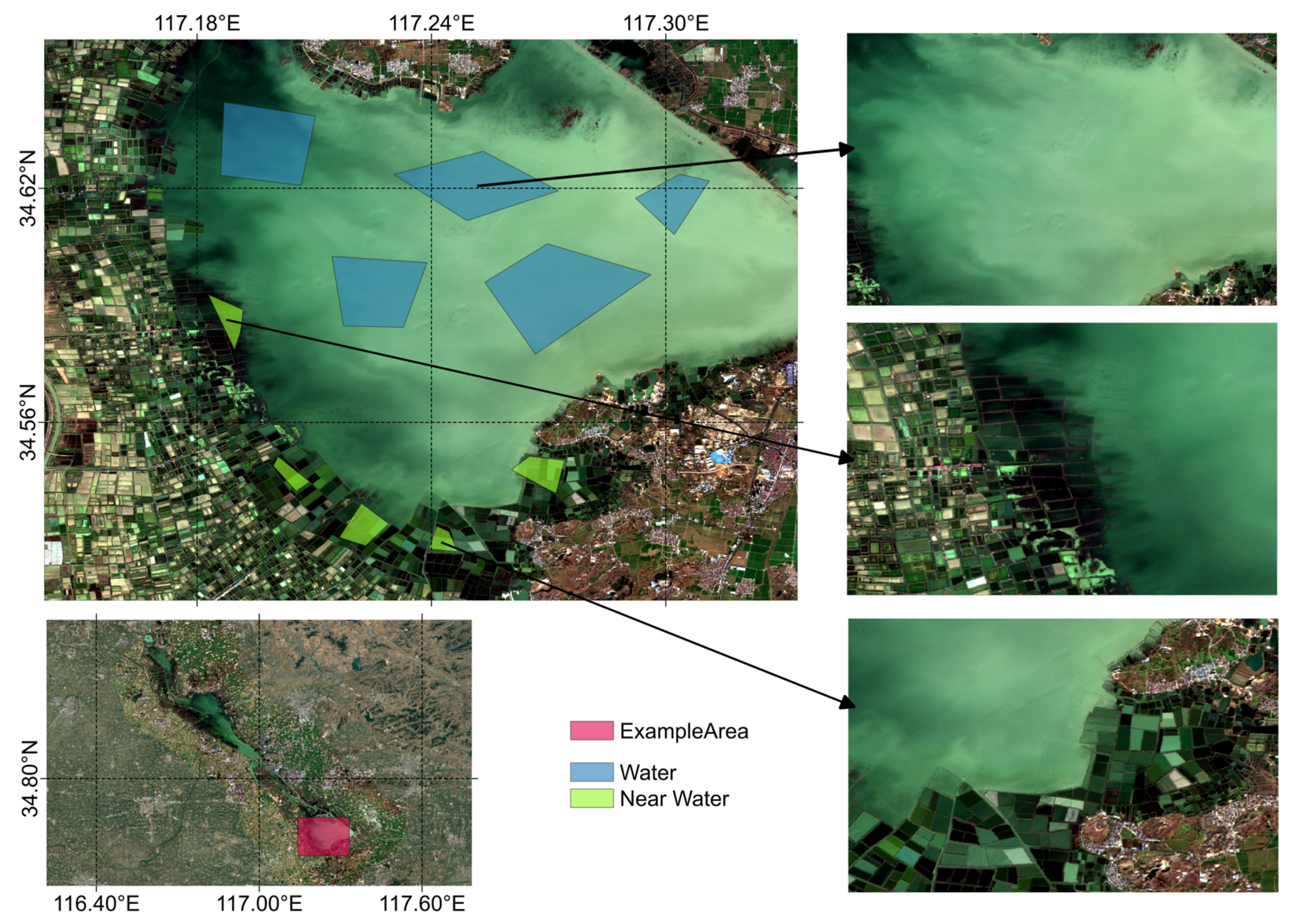
All classifications were trained using manually selected samples and executed through tile-based sampling and prediction to control computational cost and memory consumption. The training data were derived from representative land cover regions, including three major classes: water bodies, near-water land, and non-water areas. Examples of water bodies and near-water land use in the three types of areas are shown in Figure 2. After manual delineation of vector polygons, a stratified random sampling procedure was applied within each polygon to generate training samples, with approximately 1600 points per dataset (about 1000 water and 600 non-water samples). The sample selection followed two key principles: (1) spectral representativeness, ensuring coverage of various water and non-water spectral signatures, and (2) spatial balance, prioritizing clear, cloud-free regions with well-defined boundaries to minimize spectral mixing and misclassification errors. In addition, separate training sets were constructed for different seasons to adapt to changes in vegetation cover and water level, while maintaining consistency in sample size and class ratios across seasons to ensure comparability and robustness of classification performance.

Model parameters were configured following the default settings of Scikit-learn (v0.24) within GEE. For the RF classifier, 100 trees were used with 3–4 variables per split, a minimum leaf size of 10–20, and a sub-sampling fraction of 0.7, balancing accuracy and generalization capability. The CART classifier was constrained to a maximum of 64 nodes and a minimum of 10 samples per leaf node, using the same training and validation sets for consistency (

Table 2. Parameter settings of machine learning classifiers used in this study.

Model	Parameter	Value	Description
RF	Number of trees	100	Total number of decision trees
RF	Variables per split	3–4	Number of features considered at each split
RF	Minimum leaf size	10–20	Minimum number of samples per leaf node
RF	Bag fraction	0.7	Fraction of samples used for training each tree
CART	Maximum nodes	64	Maximum number of tree nodes
CART	Minimum leaf size	10	Minimum number of samples per leaf node

).

Classification accuracy was quantified using Overall Accuracy (OA) and the Kappa coefficient. To further assess the robustness of the reported accuracy metrics, a non-parametric bootstrap resampling strategy was applied to the independent test samples. For each classification result, the test dataset was repeatedly resampled with replacement, and OA and Kappa values were recalculated to approximate their empirical distributions. The 95% confidence intervals (CIs) were then derived using the percentile method. This procedure provides an estimate of the uncertainty associated with accuracy metrics and enables an evaluation of their stability with respect to sampling variability, particularly under high-accuracy classification scenarios.

The resulting classification maps were compared against NDWI-derived baseline water masks at the pixel level. The spatial distribution of three different categories—over-classified (−1), consistent (0), and under-classified (+1)—was analyzed to characterize method-specific biases. To mitigate the influence of boundary effects on accuracy assessment, a one-pixel buffer zone was established around classification edges and excluded from statistical analysis. This approach has been validated in long-term and seasonal water mapping studies as an effective strategy to reduce boundary-related uncertainty [26].

2.3. Model Portability and Generalization Verification

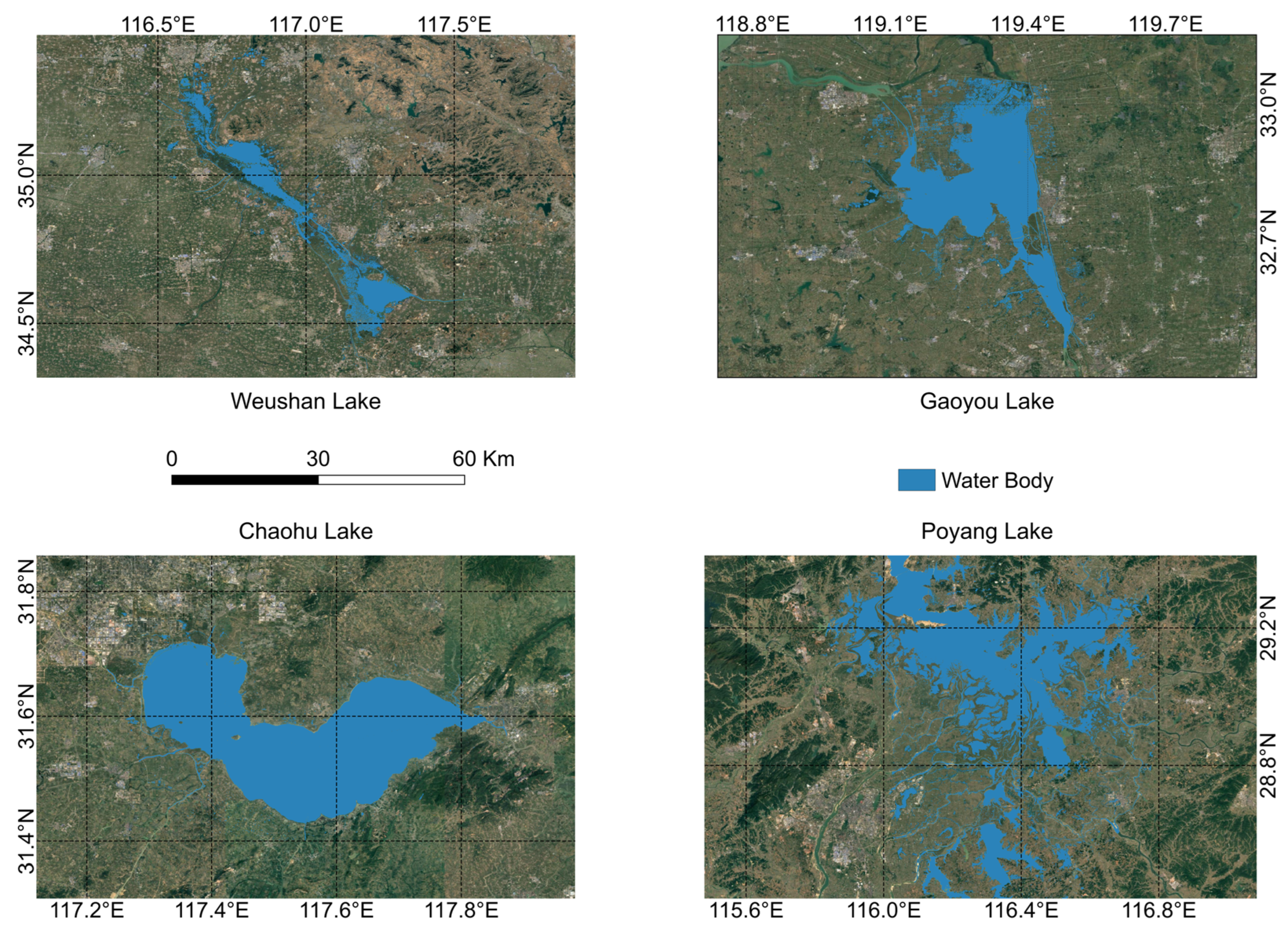
To ensure the generalization of the classification framework, this study designed model validation and transferability assessment to evaluate the applicability of the machine learning model outside the main study area. Based on the training results of the random forest (RF) classifier trained on the Weishan Lake multi-source remote sensing dataset in September 2024, the transferability and generalization of the model were validated on three representative external lake systems—Chaohu Lake, Gaoyou Lake, and Poyang Lake. These three lakes were chosen because they differ in hydrology, geomorphology, and anthropogenic factors, thus providing suitable samples for evaluating the transferability performance of the model under different environmental conditions [22]. Before applying the model, each validation area underwent the same preprocessing steps as in the Weishan Lake experiment, including Sentinel-1 and Sentinel-2 image synthesis, topographic correction, and environmental variable resampling. This ensured that the spectral, topographic, and climatic features used for prediction were consistent across all test areas. The evaluation criteria for model transferability and generalization were the same as above, and the reliability of the model extraction results was evaluated by comparing the model extraction results with the NDWI-based extraction results.

2.4. Water Body Extraction and Assessment Methods for Near-Water Areas and Water Bodies

To better characterize the transitional zones with ambiguous boundaries between water and land, this study classified the research area into three categories: water bodies, near-water land, and other land cover types, based on the combined results of water extraction using spectral indices and machine learning methods. A 30 m buffer zone was constructed around the NDWI-derived water boundaries to evaluate the spatial distribution and accuracy of the near-water class within this transition area.

To enhance the reliability and interpretability of the results, two extraction schemes were designed. The first scheme utilized only optical remote sensing data and water-related spectral indices such as NDWI, aiming to assess the performance of optical indices in delineating water boundaries with high computational efficiency and methodological simplicity. The second scheme integrated multi-source data, including optical imagery, SAR polarization features, and topographic parameters (e.g., DEM and slope), providing a multi-perspective assessment of classification performance. This integrated approach was developed to improve the robustness of classification and the accuracy of boundary delineation under challenging conditions such as cloud contamination, vegetation cover, and complex terrain [27,28].

This dual-scheme design enables a systematic comparison of the strengths and limitations of different data sources and feature combinations, offering a practical reference for selecting suitable datasets and extraction strategies in future large-scale or diverse application scenarios.

2.5. Correlation and Factor Analysis

To quantitatively assess the spatial dynamics of different land surface types and the relationships between their controlling environmental factors, this study employed a multifactor correlation and variable importance analysis framework. The selected environmental factors included: precipitation and surface temperature based on the ERA5-Land database; actual evapotranspiration (AET) based on FAO WaPOR Level 1 (AETI-D) data; and topographic factors (elevation and slope) based on the SRTM 30 m digital elevation model (DEM). Furthermore, vegetation status was represented by the Normalized Difference Vegetation Index (NDVI), calculated from cloudless Sentinel-2 images of the same observation period. These variables were chosen because they have been shown to have significant impacts on hydrological balance and surface water dynamics in previous studies [23,24].

Regarding the specific analytical methods, this study generated annual frequency maps for each of the three classification categories (water bodies, near-water bodies, and non-water bodies) based on the monthly classification results of 2024. Subsequently, stratified random sampling was performed on the three frequency maps, selecting 2000 representative points within the study area to ensure a balanced distribution of the three categories. For each sample, the mean values of environmental factors during the study period were extracted, and all samples were integrated into a comprehensive dataset for subsequent analysis.

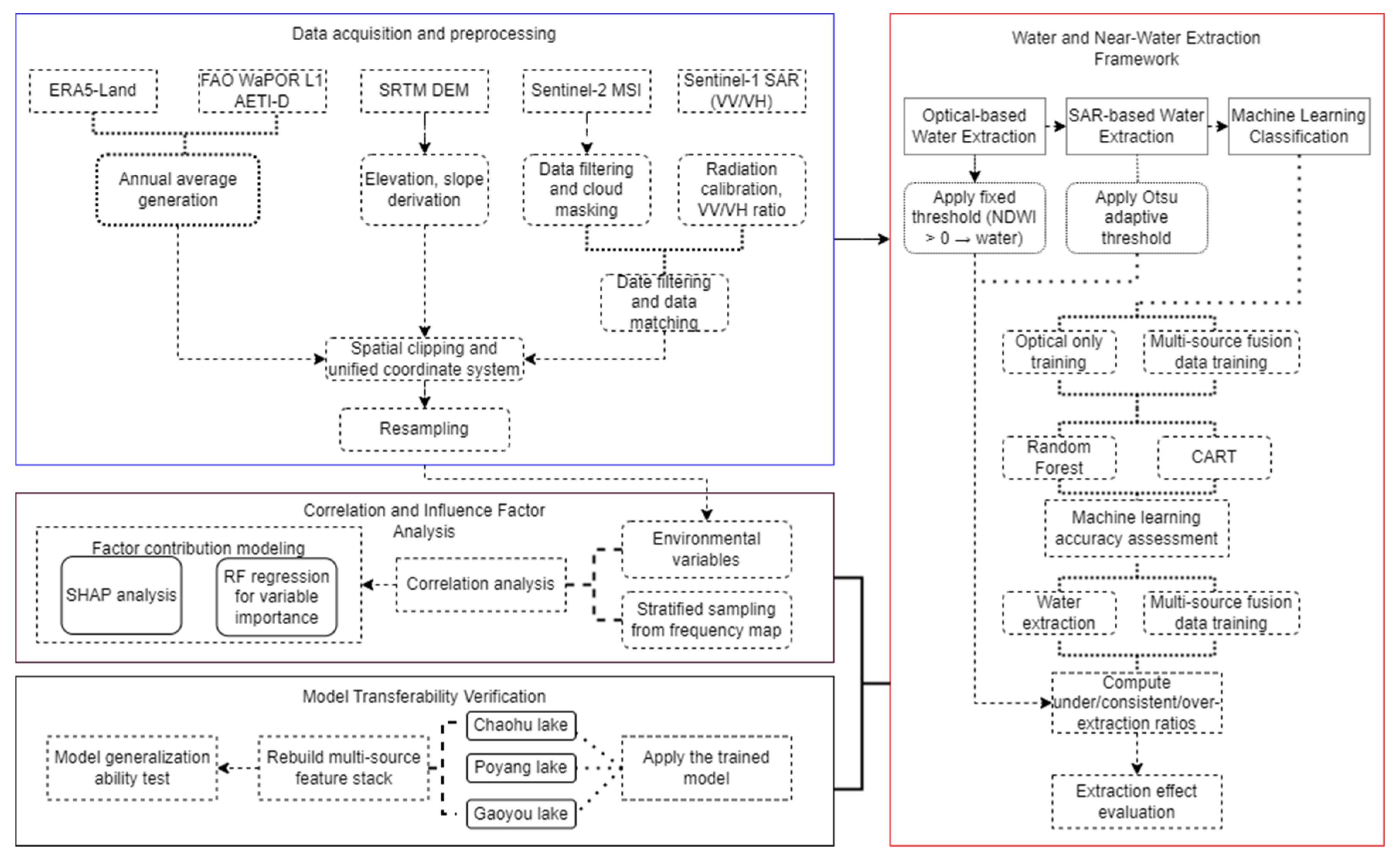
First, correlation analysis was performed to assess the linear relationship between each environmental factor and the frequency of observed categories, providing a preliminary understanding of the potential drivers of spatial variability. Subsequently, a random forest (RF) regression model was applied to quantify the relative importance of each variable to the category distribution. To enhance the interpretability of the results, SHAP (Shapley Additive exPlanations) analysis was further introduced to decompose the contributions of each variable and visualize their interactions, highlighting how vegetation activity (NDVI) and elevation (DEM) jointly influence the classification probability of water bodies. The research flowchart for this study is shown in Figure 3.

This analytical framework enables a comprehensive understanding of how climate, topography, and vegetation factors modulate the spatiotemporal variability of water bodies and near-water areas and provides a quantitative basis for assessing their hydrological responses and potential feedback mechanisms.

3. Results

3.1. Comparative Analysis of Boundary Recognition and Time Series Stability Using Optical and SAR Thresholding Methods

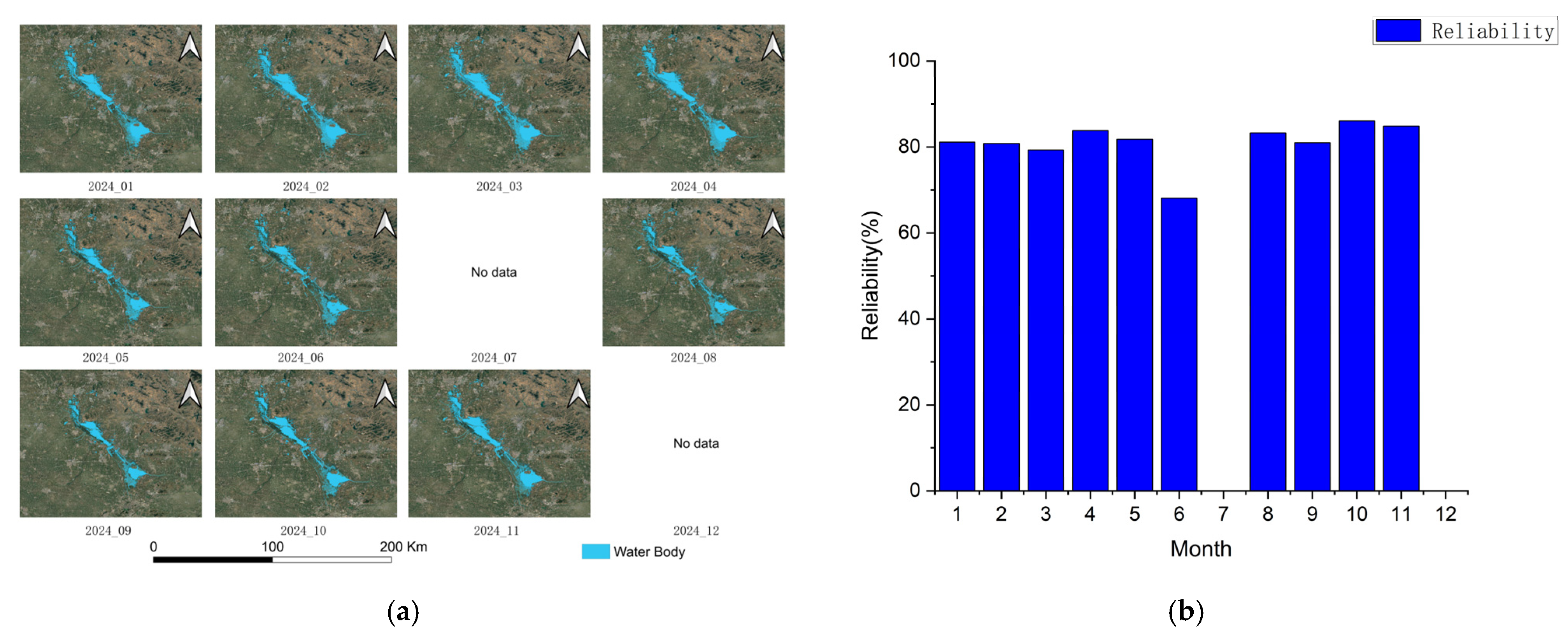
The study first extracted water bodies using the index-based approach. NDWI (B3, B8) was calculated from Sentinel-2 imagery, and pixels with NDWI > 0 were classified as water, generating a binary water mask. In the years selected for this study, there is a lack of suitable cloud cover data in July and December. However, this study believes that the corresponding two months have little impact on the research results, so the above two months are left blank (Figure 4).

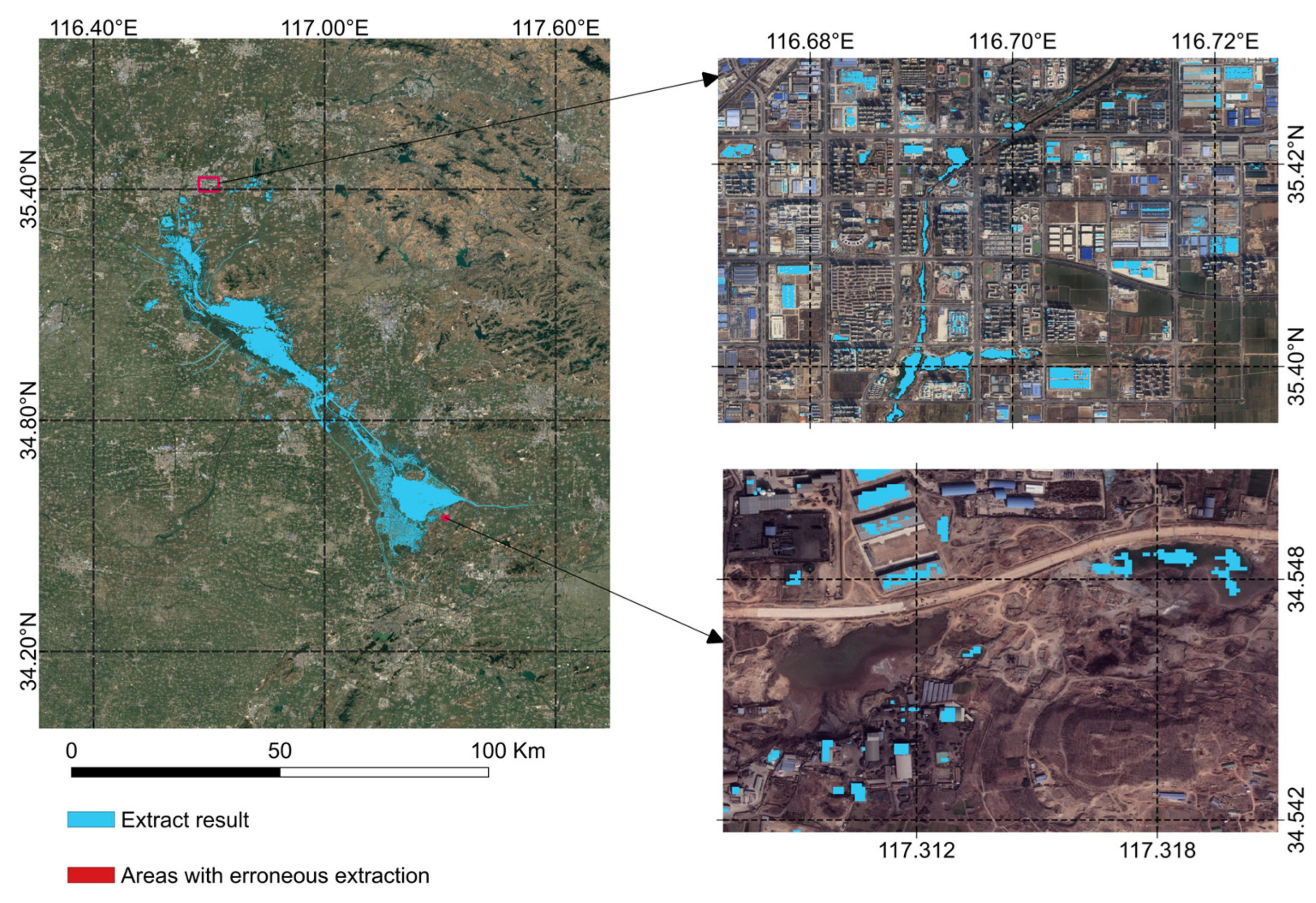
The results show that the Sentinel-2 index-based water body extraction method remains stable for most months of the year, with reliability mainly between 80% and 85%. Reliability is higher in spring and autumn, peaking at 86.05% in October, while reliability declines significantly in early summer, reaching its lowest point in June (68.14%). However, it exhibited misclassification in small water bodies and near-water agricultural areas, highlighting its limitations under complex surface conditions (Figure 5).

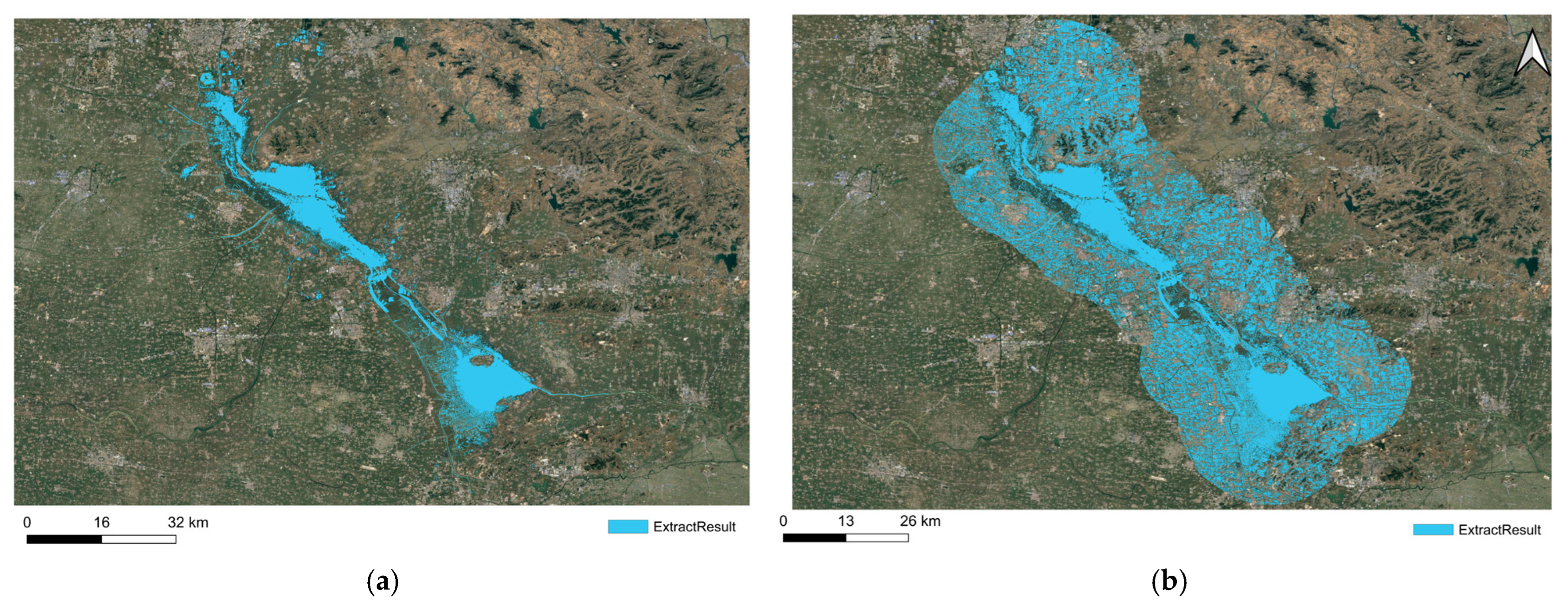
Based on Sentinel-1 VV/VH ratio data and the Otsu thresholding algorithm, the SAR-based extraction results revealed that the method could accurately identify major water bodies within localized areas but failed to maintain consistency when extended to the entire study region. In several months, classification results deviated substantially from actual water distributions, particularly in agricultural and wetland zones (Figure 6).

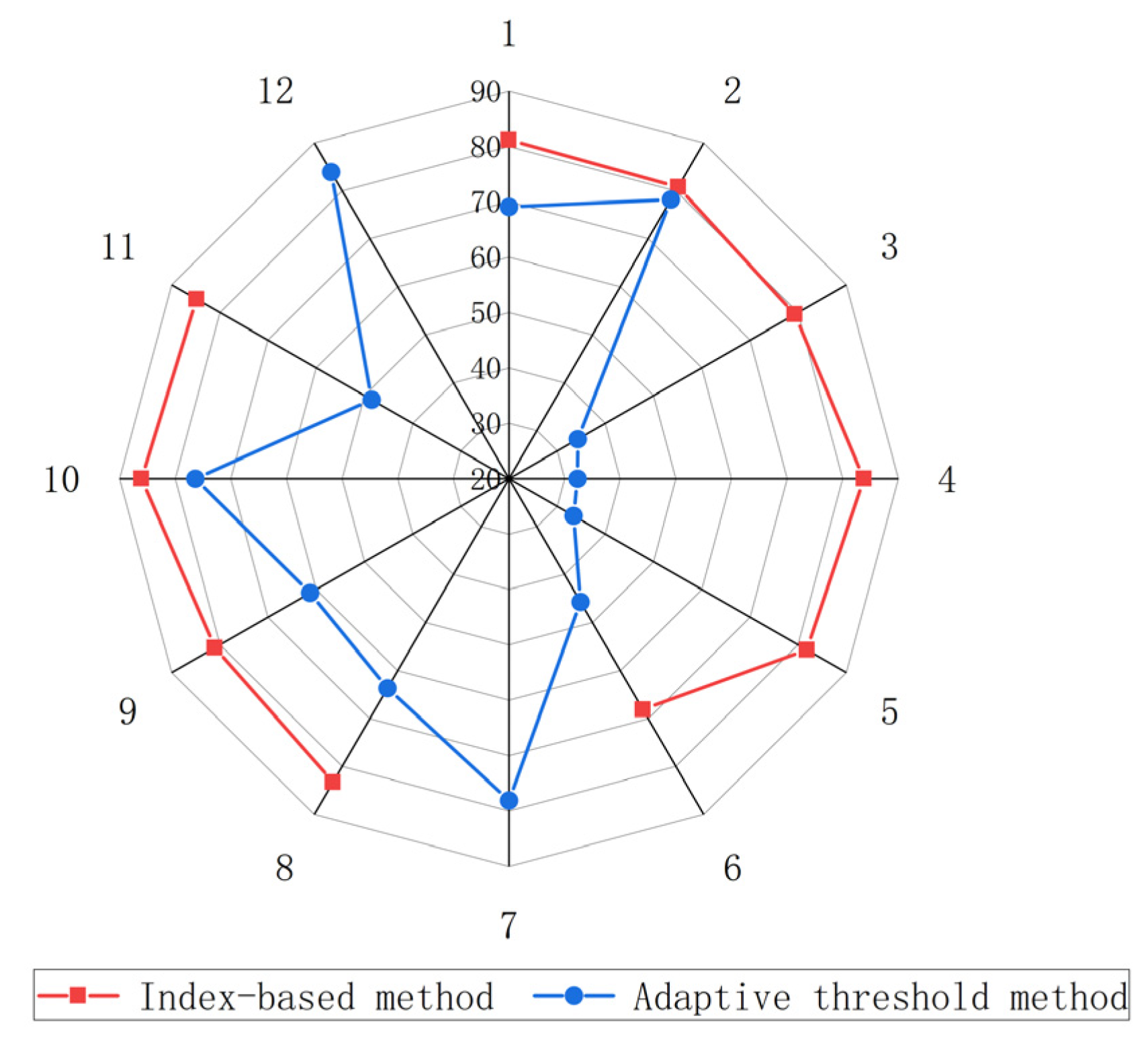
To verify the reliability of both extraction methods, the results of the NDWI-based index method and the SAR-based adaptive threshold method were compared with monthly visual interpretation maps. The spatial agreement ratio—defined as the proportion of overlapping areas between the extracted and visually interpreted results—was used to evaluate extraction accuracy and temporal consistency (Figure 6).

The results demonstrate that the index-based method achieved higher and more stable accuracy across months, with matching ratios exceeding 85% in several cases. In contrast, the adaptive thresholding method displayed considerable fluctuations, with sharp accuracy declines in certain months and satisfactory results only during specific periods. Overall, the NDWI method outperformed the SAR-based approach in both robustness and temporal stability. Hence, the NDWI results derived from Sentinel-2 imagery were regarded as reliable and consistent across months, serving as the benchmark for evaluating the credibility of subsequent machine learning classifications (Figure 7).

Conversely, while the Sentinel-1 SAR Otsu-based method also yielded satisfactory results in specific months (e.g., February and November), its overall stability was inferior, and misclassification rates increased significantly during vegetation-rich months (e.g., June and August). Therefore, the SAR–Otsu method was used in this study primarily as a supplementary reference for accuracy assessment.

3.2. Accuracy Analysis of Extraction Results from Different Machine Learning Methods

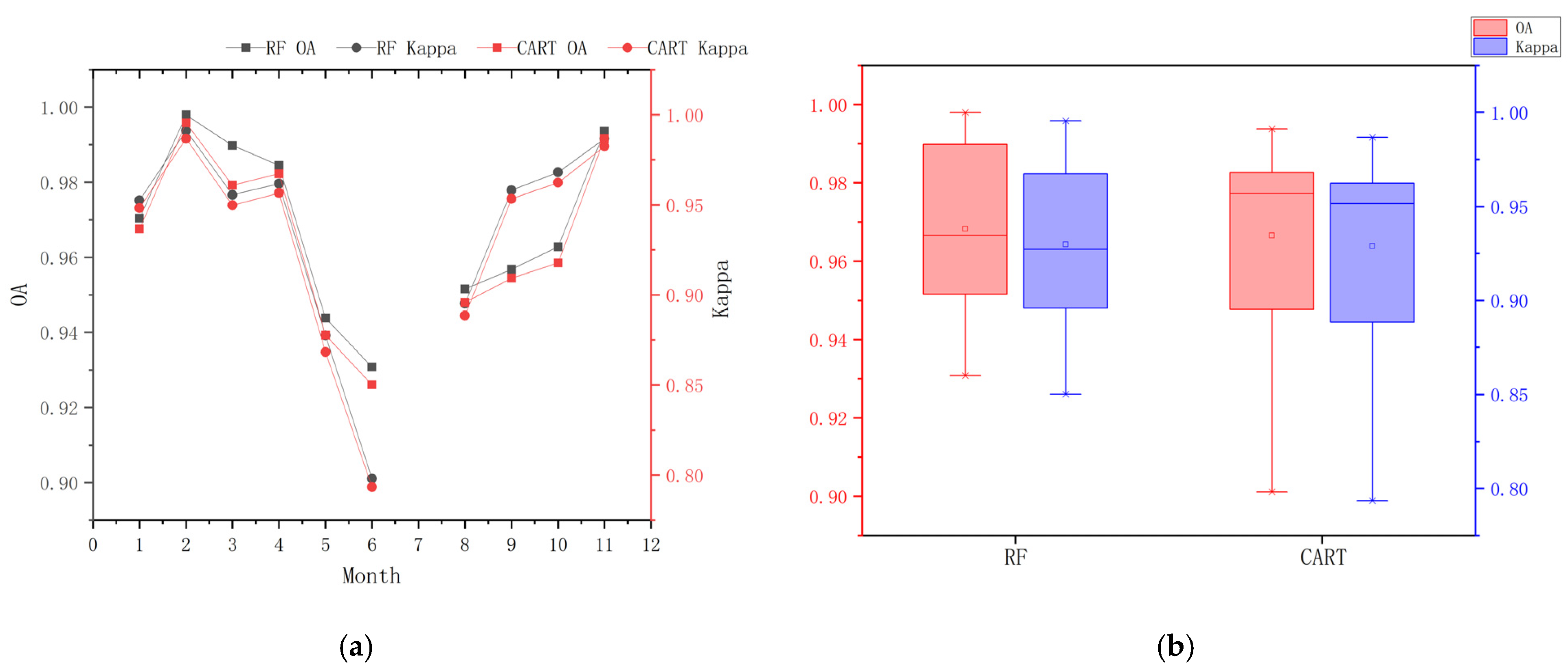
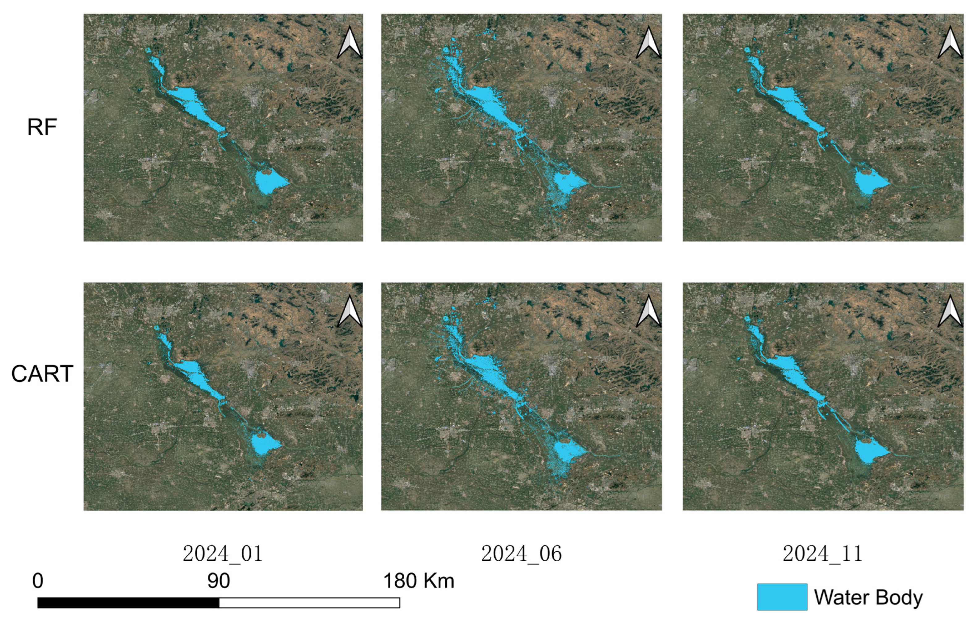
The performance of two machine learning algorithms—Random Forest (RF) and Classification and Regression Tree (CART)—was evaluated in terms of overall accuracy (OA) and Kappa coefficient. As shown in Figure 8, both methods exhibited stable performance throughout the year, with RF consistently outperforming CART.

Table 3. Machine learning monthly accuracy and reliability.

Month (2024)	RF OA (95% CI)	RF Kappa (95% CI)	CART OA (95% CI)	CART Kappa (95% CI)
January	0.9704 (0.9704–0.9704)	0.9367 (0.9367–0.9367)	0.9752 (0.9752–0.9752)	0.9483 (0.9483–0.9483)
February	0.9980 (0.9980–0.9980)	0.9956 (0.9956–0.9956)	0.9938 (0.9938–0.9938)	0.9868 (0.9868–0.9868)
March	0.9898 (0.9898–0.9898)	0.9608 (0.9608–0.9608)	0.9766 (0.9766–0.9766)	0.9498 (0.9498–0.9498)
April	0.9845 (0.9845–0.9845)	0.9672 (0.9672–0.9672)	0.9796 (0.9796–0.9796)	0.9566 (0.9566–0.9566)
May	0.9438 (0.9438–0.9438)	0.8776 (0.8776–0.8776)	0.9392 (0.9392–0.9392)	0.8683 (0.8683–0.8683)
June	0.9308 (0.9308–0.9308)	0.8502 (0.8502–0.8502)	0.9011 (0.9011–0.9011)	0.7934 (0.7934–0.7934)
July	–	–	–	–
August	0.9516 (0.9516–0.9516)	0.8959 (0.8959–0.8959)	0.9477 (0.9477–0.9477)	0.8885 (0.8885–0.8885)
September	0.9568 (0.9568–0.9568)	0.9094 (0.9094–0.9094)	0.9779 (0.9779–0.9779)	0.9534 (0.9534–0.9534)
October	0.9628 (0.9628–0.9628)	0.9177 (0.9177–0.9177)	0.9826 (0.9826–0.9826)	0.9622 (0.9622–0.9622)
November	0.9936 (0.9936–0.9936)	0.9868 (0.9868–0.9868)	0.9916 (0.9916–0.9916)	0.9824 (0.9824–0.9824)
December	–	–	–	–

summarizes the monthly classification accuracy of the RF and CART models based on optical remote sensing data in 2024, together with their corresponding 95% confidence intervals derived from bootstrap resampling. Overall, both methods achieved high classification accuracy across most months, with OA values generally exceeding 0.93 and Kappa coefficients indicating strong agreement beyond chance. The bootstrap results reveal negligible variability in OA and Kappa estimates, suggesting that the classification performance of both RF and CART models is highly stable with respect to sampling uncertainty. Seasonal differences are nevertheless observable, with relatively lower accuracy during late spring and early summer, coinciding with increased vegetation coverage and enhanced spectral confusion between water and non-water surfaces.

Specifically, the annual mean OA and Kappa coefficient of the RF classifier reached 96.5% and 0.93, respectively, whereas those of CART were 95.8% and 0.91. These results, consistent with Sun et al. [23], confirm the superior capability of ensemble learning algorithms such as RF in handling multi-source remote sensing features. Moreover, the temporal trend of accuracy showed evident seasonal variations: classification accuracy was highest in January, February, and November, when RF achieved an average OA of 98.7%. In contrast, accuracy declined markedly during months of dense vegetation (June and August), with OA dropping to 93.1% and 90.1%, respectively. This pattern indicates that lower vegetation coverage and more stable water boundaries in winter provided ideal conditions for high-accuracy classification (Figure 9).

3.3. Monthly Reliability and Accuracy Analysis of Different Machine Learning Methods

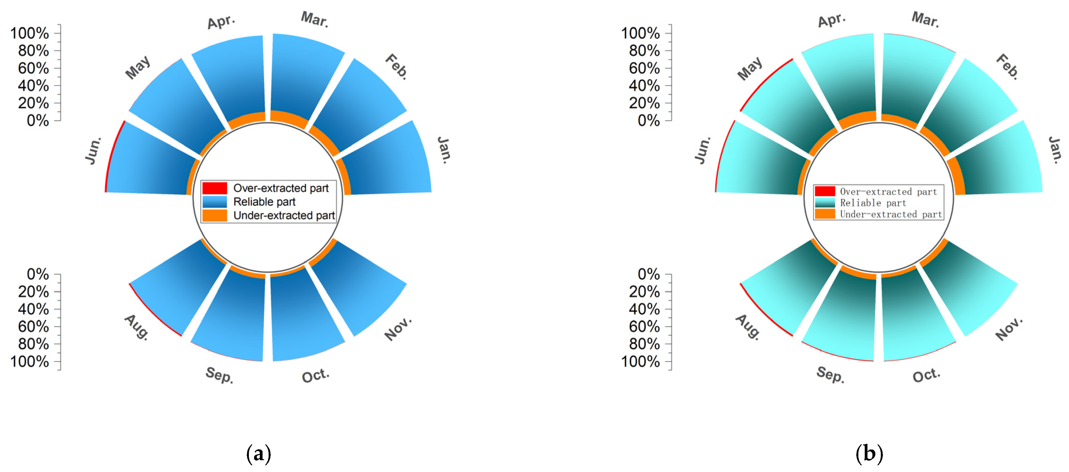
To further assess spatial classification reliability, this study introduced a “reliability” index, defined as the proportion of pixels consistent with the NDWI benchmark, and a complementary “unreliability” index that includes both over-classified and under-classified pixels (Figure 8).

Results show that the average reliability of RF (92.5%) was slightly higher than that of CART (91.2%). Both indices followed similar seasonal trends as overall accuracy. During winter months (January and November), the reliability of RF reached a maximum of 93.9% (29 November), while the minimum was observed in June (91.4%). Analysis of unreliability components indicated that CART tended to over-classify water areas during summer (e.g., 12 June, with 5.5% of pixels overclassified), likely due to its higher sensitivity to feature fluctuations. In contrast, RF exhibited a more balanced error distribution (Figure 10).

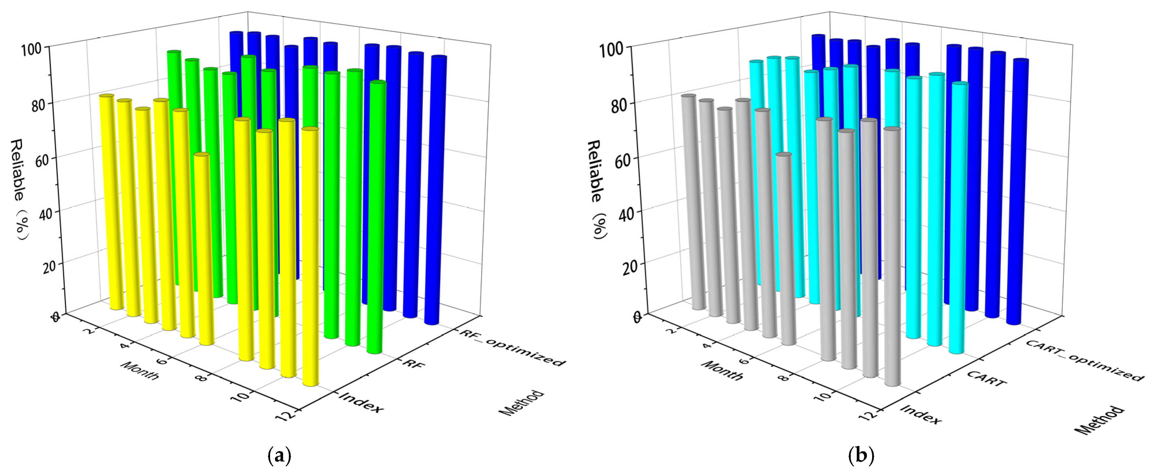
After incorporating SAR and DEM data, model reliability improved systematically (Figure 11). Multi-source data fusion effectively mitigated misclassifications caused by cloud contamination and vegetation cover, with notable improvement during the least reliable months (e.g., June). The reliability of RF increased by approximately 3.5 percentage points, accompanied by a significant reduction in unreliability. These results confirm that integrating SAR backscattering and topographic constraints substantially enhances model robustness, particularly under complex seasonal conditions.

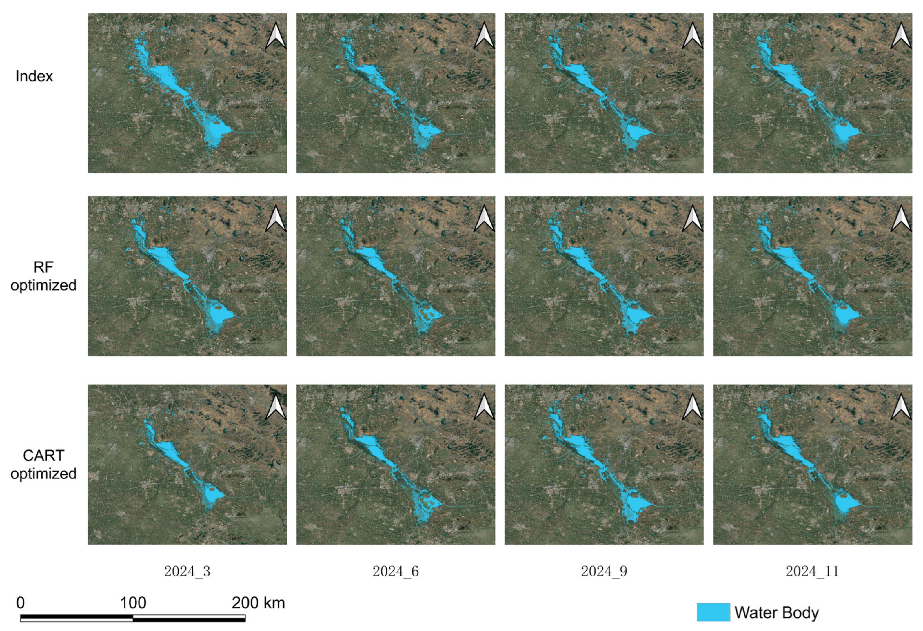
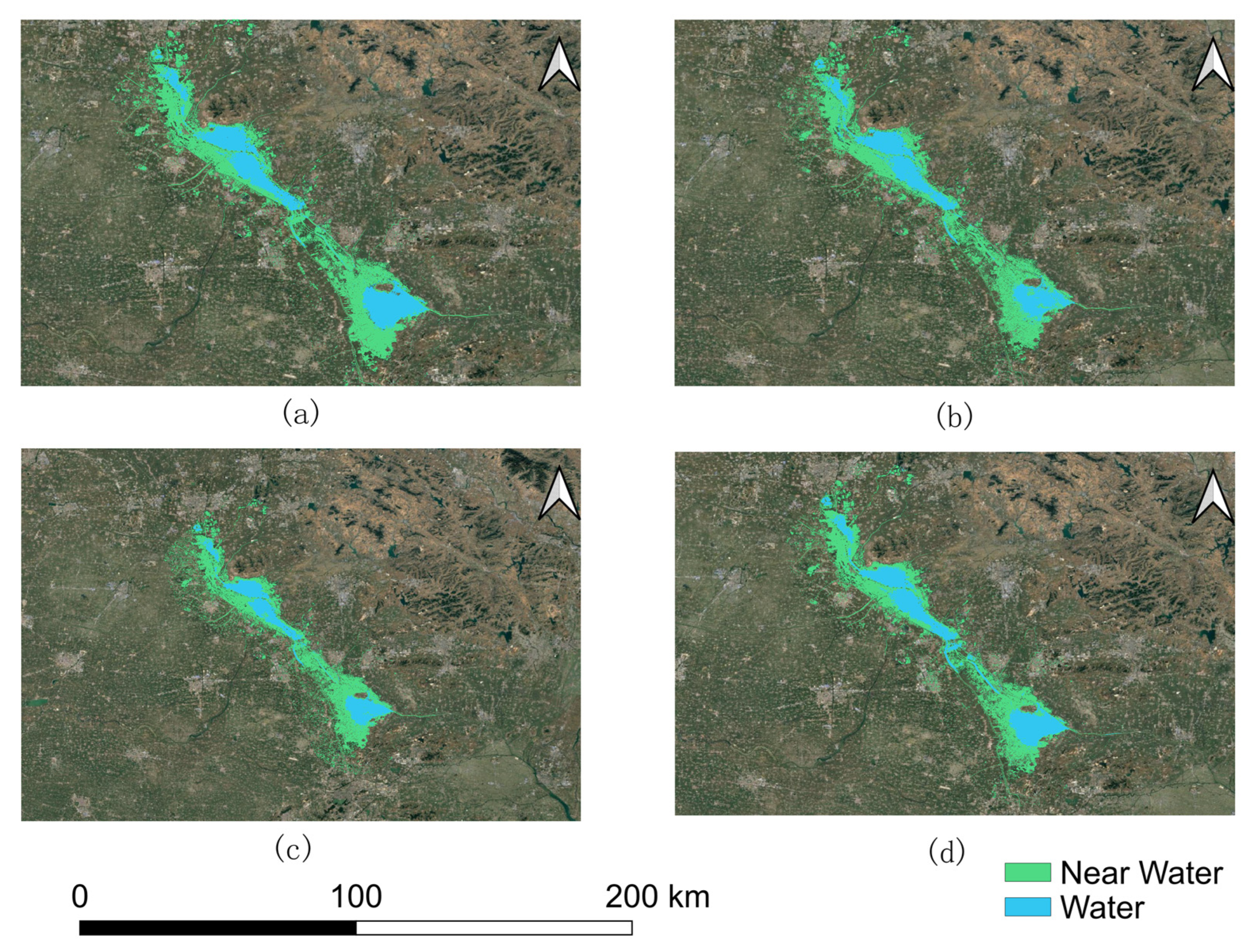
Finally, a spatial comparison of the classification maps for March, June, September, and November (Figure 12) visually supports the above quantitative findings.

3.4. Model Portability and Generalization Validation Results

To further evaluate the portability and generalization ability of the proposed multi-source fusion machine learning framework, we trained a random forest model using multi-temporal fusion data from Weishan Lake (September 2024) and applied it to three external lake systems during the same period: Chaohu Lake, Gaoyou Lake, and Poyang Lake.

Generalization validation results show that the model maintains high spatial consistency across all test areas, with consistency rates of 98.88%, 94.93%, and 97.42% for Chaohu Lake, Gaoyou Lake, and Poyang Lake, respectively (

Table 4. Generalization verification results.

Verify Area	Over-Extract Part (%)	Under-Extract Part (%)	Reliable Part (%)
Chaohu Lake	0.82	0.30	98.88
Gaoyou Lake	4.75	0.31	94.93
Poyang Lake	1.44	1.13	97.42

).

A slight underestimation was observed in shallow or seasonally flooded shoreline areas, while a slight overestimation was observed in densely vegetated wetland areas, possibly due to the spectral similarity between aquatic vegetation and open water bodies (Figure 13).

These findings confirm that the proposed classification framework has strong generalization ability under different hydrological and environmental conditions. The stability of water body and near-water area segmentation under different topographic and climatic conditions indicates that the fusion of optical, radar, and topographic information effectively mitigates the effects of sensor noise and local surface heterogeneity.

3.5. Analysis of Near-Water Area Extraction Results

Using the three-class Random Forest classification results derived from multi-source data (Sentinel-1 + Sentinel-2 + DEM), this study quantified the spatial proportion and temporal variability of the near-water land category, which represents the transitional zone between water and terrestrial surfaces.

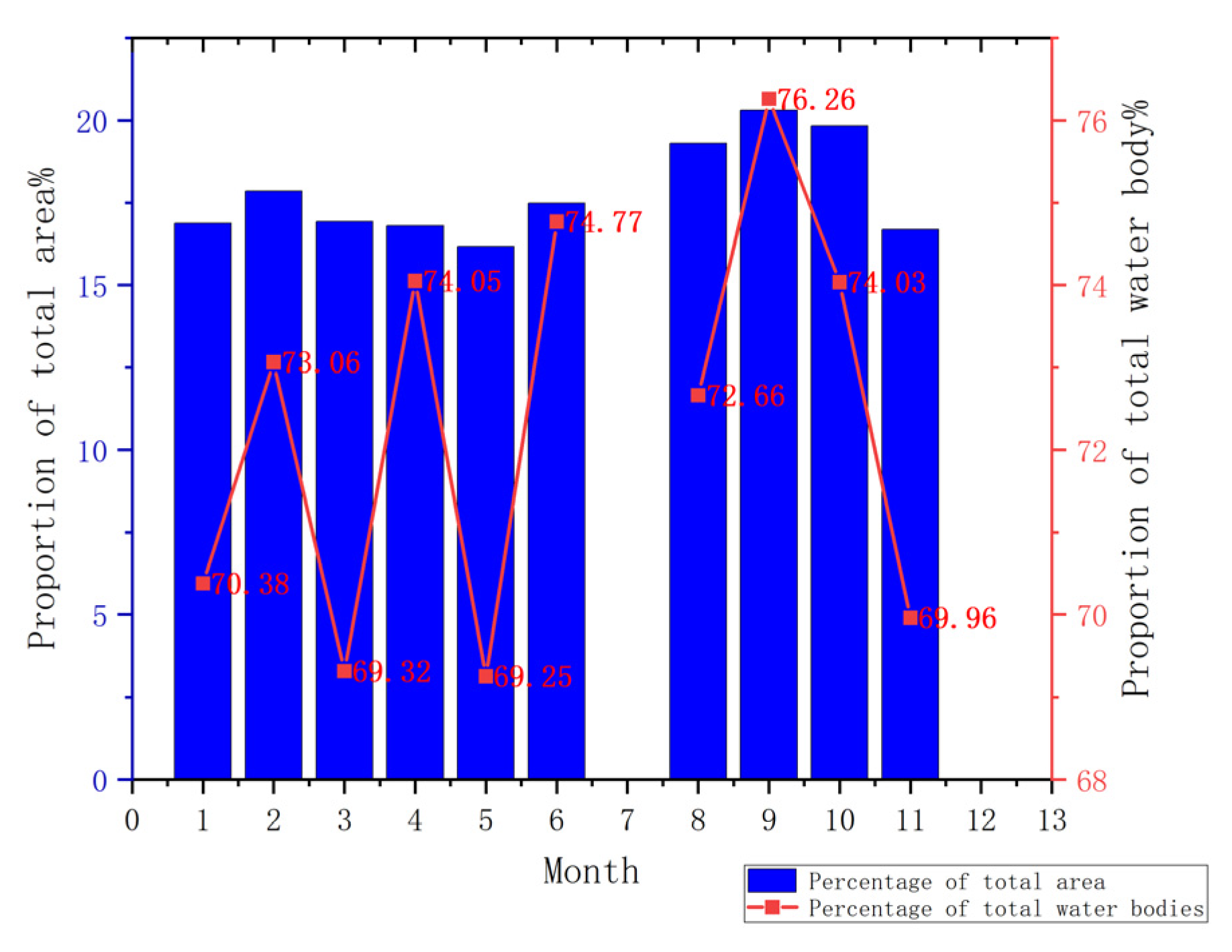
As illustrated in Figure 14, the proportion of near-water land pixels relative to the total area fluctuated across months, with an annual average of 17.8%. The maximum value occurred in September (20.3%), and the minimum in May (16.2%).

In addition, the ratio of near-water pixels to the combined total of water and near-water pixels (Near-water/[Water + Near-water]) revealed the relative dominance of transitional zones within the overall water-related area. The annual mean value of this ratio was 72.3%, peaking at 76.3% in September and declining to 69.3% in May (Figure 14).

Both metrics demonstrated highly consistent seasonal patterns (Figure 15). From January to May, the ratios showed a downward trend, reaching their lowest levels in May. Starting in June, both indicators increased markedly and remained high during August–October, with September representing the annual peak. Thereafter, the values declined in November, returning to levels comparable to those observed at the beginning of the year.

3.6. Correlation and Influencing Factor Analysis Results

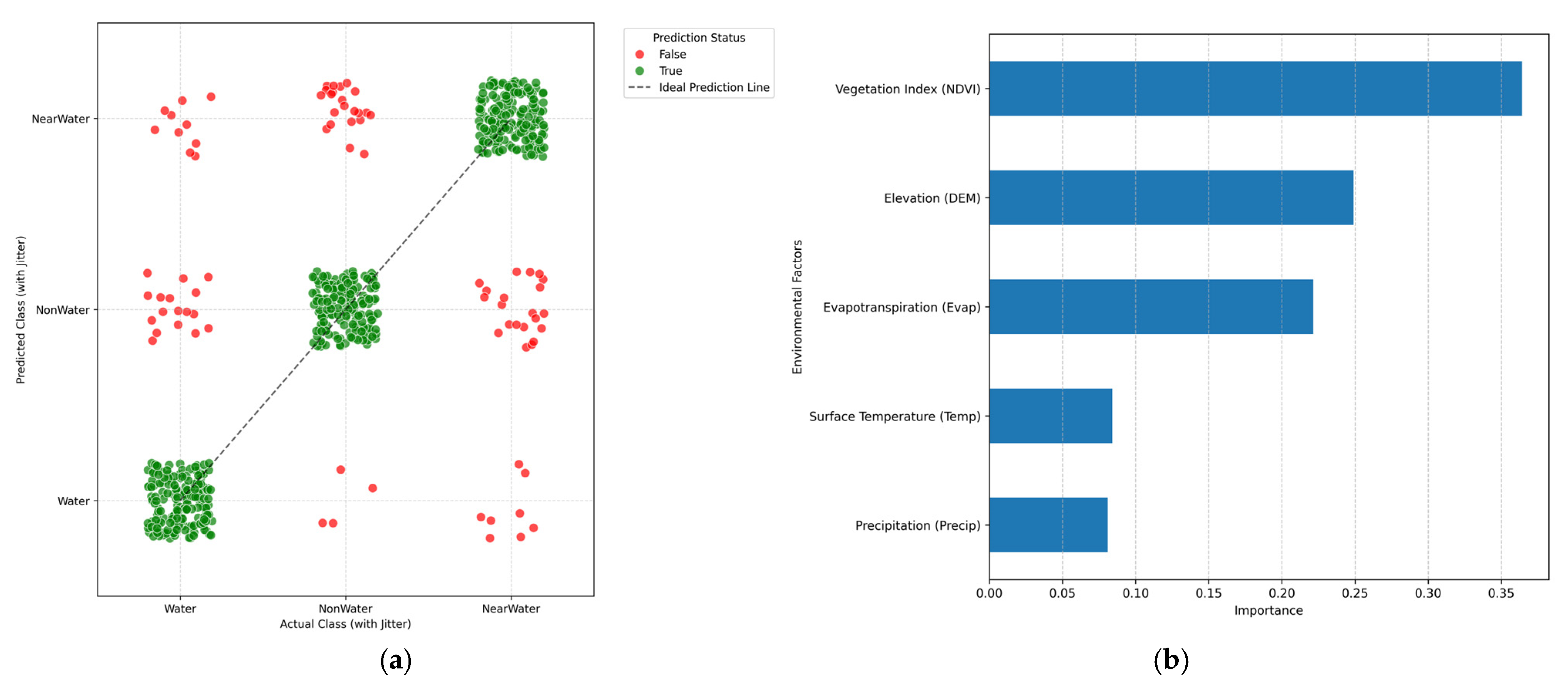
To further quantify the relationship between environmental variables and classification results, this study applied a random forest (RF) model trained on multi-source remote sensing data to evaluate the relative influence of key factors such as precipitation, surface temperature (Temp), evapotranspiration (Evap), topography (DEM), and vegetation (NDVI). The model achieved an overall classification precision of 0.863, maintaining balanced precision and recall across the three categories of water bodies, near-water bodies, and non-water bodies, indicating stable predictive performance under different surface conditions. The results are shown in Figure 16.

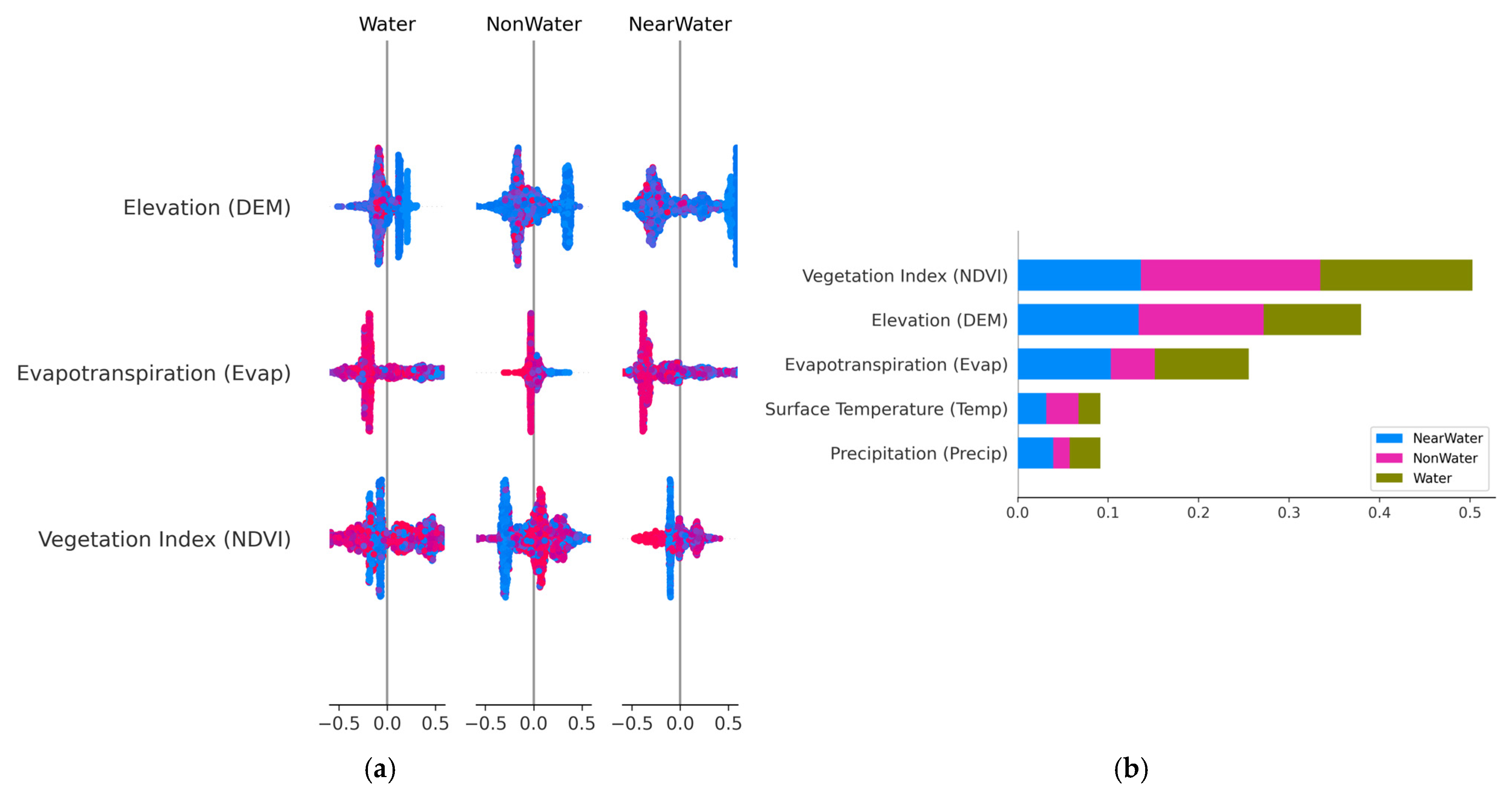
Feature importance analysis revealed that vegetation (0.364) and topography (0.249) were the primary predictors, followed by evapotranspiration (0.222), while surface temperature (0.084) and precipitation (0.081) had relatively weaker influences. These results suggest that vegetation cover and topographic changes have a stronger controlling effect on the spatial distribution of water bodies and near-water bodies than short-term hydroclimatic fluctuations. The results are shown in Figure 17.

SHAP analysis further decomposed the model output to the category level. For water body categories, vegetation and topographic factors exhibited the highest mean SHAP values, highlighting their dominant role in determining water body presence. In non-water and near-water body categories, vegetation remained the most influential factor, but topographic factors and evaporation also significantly contributed to distinguishing transition zones. The results are shown in Figure 18.

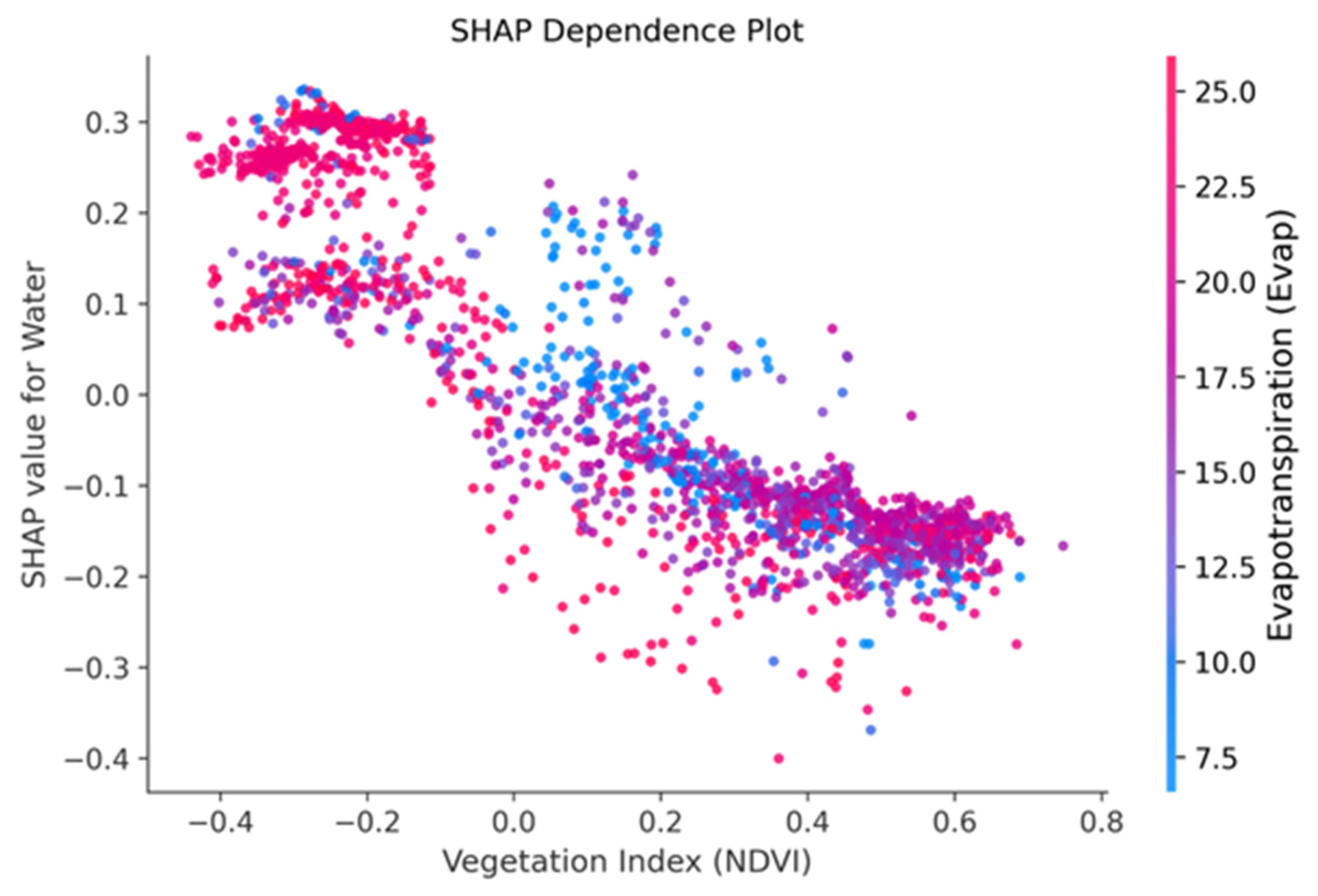
SHAP dependency plots for vegetation and topographic factors show that higher vegetation density combined with lower topography significantly reduces the probability of water body classification, reflecting the interaction between vegetation density and topographic depression.

Overall, these results confirm that the combined effects of vegetation dynamics, topographic structure, and surface energy exchange dominate the spatial variability of water-near-water body transition zones. The observed factor sensitivities provide a quantitative basis for explaining the physical consistency of the model, which will be discussed in more detail in the next section.

4. Discussion

This study systematically evaluated the performance of multi-source remote sensing data and various extraction methods in identifying complex lake water bodies and near-water land, integrating both methodological assessment and spatiotemporal dynamics analysis. The discussion focuses on four aspects: method applicability, the value and challenges of multi-source data fusion, spatiotemporal dynamics of water and near-water land, and research limitations.

4.1. Performance and Applicability of Different Water Extraction Methods

The results show significant performance differences among different remote sensing methods in water body extraction. Optical index-based methods (e.g., NDWI) perform well in identifying large, static water bodies; however, their reliability drops significantly in complex environments such as near-water agricultural land and wetlands. This limitation is primarily related to spectral ambiguity near lake margins, where mixed surface conditions reduce class separability [29].

In contrast, SAR-based threshold segmentation methods demonstrate a clear advantage in rapidly identifying small water bodies [10]. Nevertheless, SAR backscattering similarity between inundated cropland, paddy fields, and open water can lead to systematic overestimation at large spatial scales, highlighting the sensitivity of SAR-only approaches to land use context and scattering mechanisms [30,31,32]. This confirms that SAR-only approaches remain sensitive to land use context and scattering mechanisms.

For machine learning methods, random forests (RF) have higher machine learning accuracy than single decision trees (CART), which suggests that they are better at handling high-dimensional features and suppressing noise. This advantage can be attributed to RF’s ensemble structure, which reduces sensitivity to noise and feature redundancy in high-dimensional inputs [32,33]. However, the occasional performance fluctuation observed when incorporating multi-source features suggests that increased dimensionality does not automatically guarantee improved accuracy, consistent with findings reported in related studies [34,35,36].

4.2. The Value and Challenges of Multi-Source Remote Sensing Data Fusion

Unlike conventional studies that focus on single-sensor optimization, the proposed framework emphasizes functional complementarity among optical, SAR, and topographic data rather than simple feature stacking. Within this framework, optical imagery enhances spatial detail, SAR ensures temporal continuity under adverse atmospheric conditions, and DEM-derived terrain constraints reduce terrain-related misclassification.

A key methodological innovation lies in the integration of a tri-class classification scheme (“Water–Near-Water Land–Non-Water”), which explicitly represents transitional lake–land zones that are commonly ignored in binary water mapping frameworks. This structural refinement enhances the interpretability and stability of classification outputs, particularly in irrigation-dominated lake systems.

Furthermore, multi-seasonal training strategies improve temporal robustness by accounting for vegetation phenology and hydrological variability, allowing the framework to maintain stable performance across contrasting seasonal conditions. This strategy enables stable performance across contrasting seasonal conditions in agricultural lake environments [37,38].

4.3. Spatiotemporal Dynamic Characteristics of Water Bodies and Near-Water Land Uses

The extracted water and near-water land distributions reveal pronounced seasonal dynamics. Overall, extraction accuracy was higher during winter months, while noticeable declines occurred in summer, consistent with increased vegetation density and irrigation activities [39]. This seasonal contrast highlights the importance of explicitly modeling vegetation–water interactions when monitoring agricultural lakes.

By introducing “near-water land” as an independent class, this study revealed the transitional nature between water and terrestrial environments. Near-water land constituted a large proportion of water-related areas and reached a seasonal maximum in late summer, reflecting intensified irrigation and enhanced hydrological connectivity. Similar patterns have been reported in regional wetland dynamics studies [40,41].

These findings indicate that near-water land dynamics provide critical information beyond traditional water extent products. Monitoring these transitional zones offers practical value for irrigation scheduling, wetland conservation, and early warning of hydrological stress, particularly in intensively managed agricultural landscapes [42,43,44].

4.4. Environmental Controls on Water and Near-Water Distribution

Random forest (RF) and SHAP factor importance analysis showed that vegetation (NDVI) and topography (DEM) were the dominant environmental factors controlling the spatial differentiation of water bodies and waterfront transition zones. The dominance of NDVI explains the reduced classification accuracy during peak growing seasons, when dense vegetation masks underlying water signals.

The importance of topography (DEM) reflects the basic laws of hydrological processes, with low-lying areas being areas where water naturally accumulates. SHAP analysis further reveals the nonlinear interaction effect between vegetation and topography: in pixels combining high vegetation cover and low elevation topography, the probability of the model classifying them as water bodies is significantly reduced. This precisely explains the classification uncertainty in complex scenarios such as riparian marshes and seasonally flooded agricultural areas, which is related to the widespread distribution of near-water agricultural land in the study area [45,46].

In contrast, evaporation, as a comprehensive indicator of surface energy and water exchange, is more important than precipitation and temperature, reflecting the direct regulatory effect of evapotranspiration on shallow water bodies and soil moisture, which is closely related to the widespread agricultural irrigation activities in the study area [47].

4.5. Research Limitations and Future Prospects

Despite its contributions, this study has several limitations. First, the spatial and temporal distribution of training samples was not fully balanced across land cover types and seasons, which may limit model generalizability in specific periods [17]. Second, the inclusion of high-dimensional multi-source features increases the risk of overfitting and computational burden.

Future work should focus on: (1) implementing feature selection and regularization strategies to reduce redundancy and overfitting [34,35,36]; (2) assessing computational efficiency to balance accuracy gains and processing costs; and (3) integrating physically informed or hybrid learning models to enhance interpretability in complex agro-hydrological environments [48,49].

5. Conclusions

This study integrated multi-temporal Sentinel-1 SAR, Sentinel-2 optical imagery, and terrain data to systematically compare the applicability of optical index methods, SAR thresholding, and multiple machine learning algorithms in complex lake environments. The results revealed distinct differences among algorithms in terms of accuracy, stability, and misclassification mechanisms. Multi-source remote sensing data fusion significantly enhanced the robustness and precision of water body extraction, effectively overcoming the limitations of single optical imagery affected by cloud cover and temporal variability, and verified the reliability and scalability of multi-source synergistic approaches for water identification.

Based on these findings, a three-class classification framework was developed using the Random Forest algorithm, incorporating “near-water land” as an independent category to overcome the constraints of conventional binary water–non-water extraction models. This framework enabled refined delineation and dynamic characterization of the water–wetland–land continuum. The results demonstrated that lake boundaries exhibit not a simple linear expansion or contraction, but a seasonal pulsation process driven jointly by hydrological rhythms and human activities. The transitional zone expanded markedly during summer and autumn and stabilized during winter. These insights advance the understanding of seasonal water dynamics and provide a novel methodological perspective for long-term temporal monitoring.

Overall, the proposed multi-source fusion and three-class classification framework demonstrates strong transferability and broad applicability across complex wetland and irrigation-lake environments. By enabling more precise estimation of irrigation water volume and near-water dynamics, the framework contributes to sustainable agricultural water allocation, improved irrigation planning, and the long-term management of agro-hydrological systems.