Lane Change Trajectory Planning for Intelligent Electric Vehicles in Dynamic Traffic Environments: Aiming at Optimal Energy Consumption

Abstract

With the reduction in battery costs and the widespread application of artificial intelligence, the adoption of new-energy vehicles is accelerating. Integrating energy consumption optimization into the process of intelligent development is of great significance for sustainable development. This paper, considering the regenerative braking characteristics of electric vehicles and the time-varying nature of surrounding obstacle vehicles during lane changes, proposes a segmented real-time trajectory-planning method combining optimal control and quintic polynomials. At the beginning of the lane change, a safe intermediate position is calculated based on the speed and position information of the ego vehicle and the leading obstacle vehicle in the current lane. The trajectory optimization problem from the starting point to the intermediate position is formulated as an optimal control problem, resulting in the first segment of the trajectory. Upon reaching the intermediate position, the endpoint range is determined based on the speed and position information of the leading and trailing obstacle vehicles in the target lane. Multiple trajectories are then generated using quintic polynomials, and the optimal trajectory is selected as the second segment of the lane-changing trajectory. Experimental results from a driving simulator show that the proposed method can reduce energy consumption by approximately 40%.

1. Introduction

Energy-efficient trajectory planning for electric vehicles plays a crucial role in advancing sustainable development. First, energy-saving trajectory planning can effectively reduce energy consumption and extend the driving range of electric vehicles. Second, it helps decrease carbon emissions and promotes the development of a green transportation system. With the growing adoption of electric vehicles, intelligent trajectory planning can lower the overall energy consumption of vehicles, reducing greenhouse gas emissions and supporting global efforts to combat climate change. Additionally, proper trajectory planning can reduce the strain on batteries, extend their lifespan, and, consequently, prolong the service life of electric vehicles, reducing resource consumption and promoting sustainable resource utilization. Overall, energy-efficient trajectory planning for electric vehicles not only enhances their overall performance and economic efficiency but also provides technical support for achieving low-carbon and green transportation, making it a significant measure in promoting global sustainable development.

Vehicle lane-changing maneuvers can greatly affect roadway efficiency and safety [1]. With the continuous progress in autonomous driving technology, automated lane changing can reduce traffic congestion and improve traffic flow efficiency. A full lane-changing maneuver consists of three stages: decision-making, trajectory design, and control execution [2]. As an important link connecting lane-change decisions and tracking control, the challenge of designing a trajectory that ensures safety, comfort, and energy efficiency has garnered growing interest within the academic community.

The research achievements in the domain of lane-changing trajectory planning are abundant, and the research methods can mainly be categorized into the following four types: search-based planning methods, artificial potential field methods, parameterized curve-based methods, and sampling-based methods [3]. Search-based methods primarily use algorithms such as A* [4,5,6], Dijkstra [7,8], and D* [9]. The strength of this method lies in its adaptability and ability to adapt to different requirements, while its main drawback is poor real-time performance, making it unsuitable for high real-time demands. The artificial potential field method [10], proposed by Khatib [11], is simple and efficient; however, its limitations include the failure to account for vehicle dynamics constraints and the difficulty in constructing potential fields in complex scenarios. The sampling-based methods, including RRT [12,13,14] and PRM [15], have strong sampling search capabilities, but they suffer from the drawback of being highly blind in their sampling process, resulting in significant computational costs. The parameterized curve-based methods include polynomial lane-changing algorithms [16], arc-based lane-changing algorithms [17], and trapezoidal curve-based lane-changing algorithms [18]. These methods are computationally efficient, highly accurate, and exhibit good real-time performance [19]. In dynamic lane-changing scenarios, real-time constraints can lead to planning errors due to computation time; hence, algorithms with a better real-time performance are more advantageous. Currently, parameterized curve-based methods are widely used in vehicle trajectory planning research for dynamic scenarios. To ensure safe lane changes in complex scenarios, Tang et al. [20] and others used quintic polynomials to generate multiple lane-changing trajectory clusters. Then, based on collision risk and comfort, they selected a suitable reference trajectory, which guided the construction of a piecewise quintic polynomial. The trajectory optimization problem was represented as a nonlinear programming problem with constraints to find the optimal trajectory. Li et al. [21] designed a linear time-varying MPC controller based on the vehicle dynamics model. They introduced an obstacle avoidance function that adjusts its value according to the distance between the vehicle and nearby obstacles, enabling the planning of a trajectory that both avoids obstacles and minimizes trajectory deviation. Luo et al. [22] proposed a dynamic approach for automated lane changing by utilizing vehicle-to-vehicle communication. In order to optimize the performance in real time of lane-changing trajectory planning, Niu et al. [23] introduced a dual quintic polynomial lane-changing method. Similar research includes Hu et al. [24], who proposed a dual quintic polynomial overtaking model for bidirectional dual-lane obstacle-avoidance overtaking scenarios, and Chen et al. [25], who used 3D Bezier curves for the trajectory design for lane changes and divided the trajectory into two segments to avoid collisions with obstacles. Wang et al. [26] employed a Hunting Coefficient (HC) indicator applied to a wayside hunting detection system (WHDS), providing an innovative method for condition monitoring.

With the in-depth development of trajectory-planning research, an increasing number of scholars aim to not only avoid obstacles during the trajectory design for lane changes but also reduce lane-changing energy consumption, to consider the economic efficiency of the trajectory design for lane changes. The primary idea in this area of research is to treat energy consumption as the cost function and calculate the lane-changing trajectory that optimizes energy efficiency [27]. Furthermore, various factors such as different driving styles [28,29], travel distance, environmental temperature, traffic conditions, and road gradients all impact energy consumption, with smoother lane-changing trajectories generally resulting in lower energy consumption [30]. Therefore, existing research also considers the effects of different driving styles [31] and driving demands [32] on lane-changing energy consumption. However, most studies typically assume that lane-changing scenarios are static or quasi-static [33]. In reality, in complex road scenarios the obstacle vehicles are not necessarily maintaining a consistent speed; during the lane-changing process between vehicles, the surrounding obstacle vehicles may suddenly accelerate or decelerate; planning algorithms have difficulty in generating real-time trajectories according to the dynamic changes in road information in real time to guarantee that the vehicle is traveling continuously [34].Therefore, it is necessary to update the real-time lane-change trajectory to account for the dynamic changes in the surrounding obstacle vehicles. In conclusion, developing a method for generating lane-changing trajectories that meets safety standards, real-time performance, economic efficiency, and comfort in dynamic traffic scenarios has become a current research hotspot. To address this, a real-time trajectory-planning method combining optimal control and quintic polynomials is proposed for intelligent electric vehicles in dynamic traffic scenarios, aiming to optimize energy efficiency while using comfort as a constraint. The trajectory adjusts in real time through piecewise planning.

The primary contributions of this paper are as follows:

• Considering the dynamic time variation of the surrounding obstacles, a segmented trajectory planning model is developed to dynamically adjust the trajectory of lane changing;
• Considering the braking energy recovery characteristics of electric vehicles, a cost function that simultaneously considers economy, comfort, efficiency, and safety risks is constructed;
• The impact of various lane-changing factors on the energy usage of electric vehicle lane changes is analyzed.

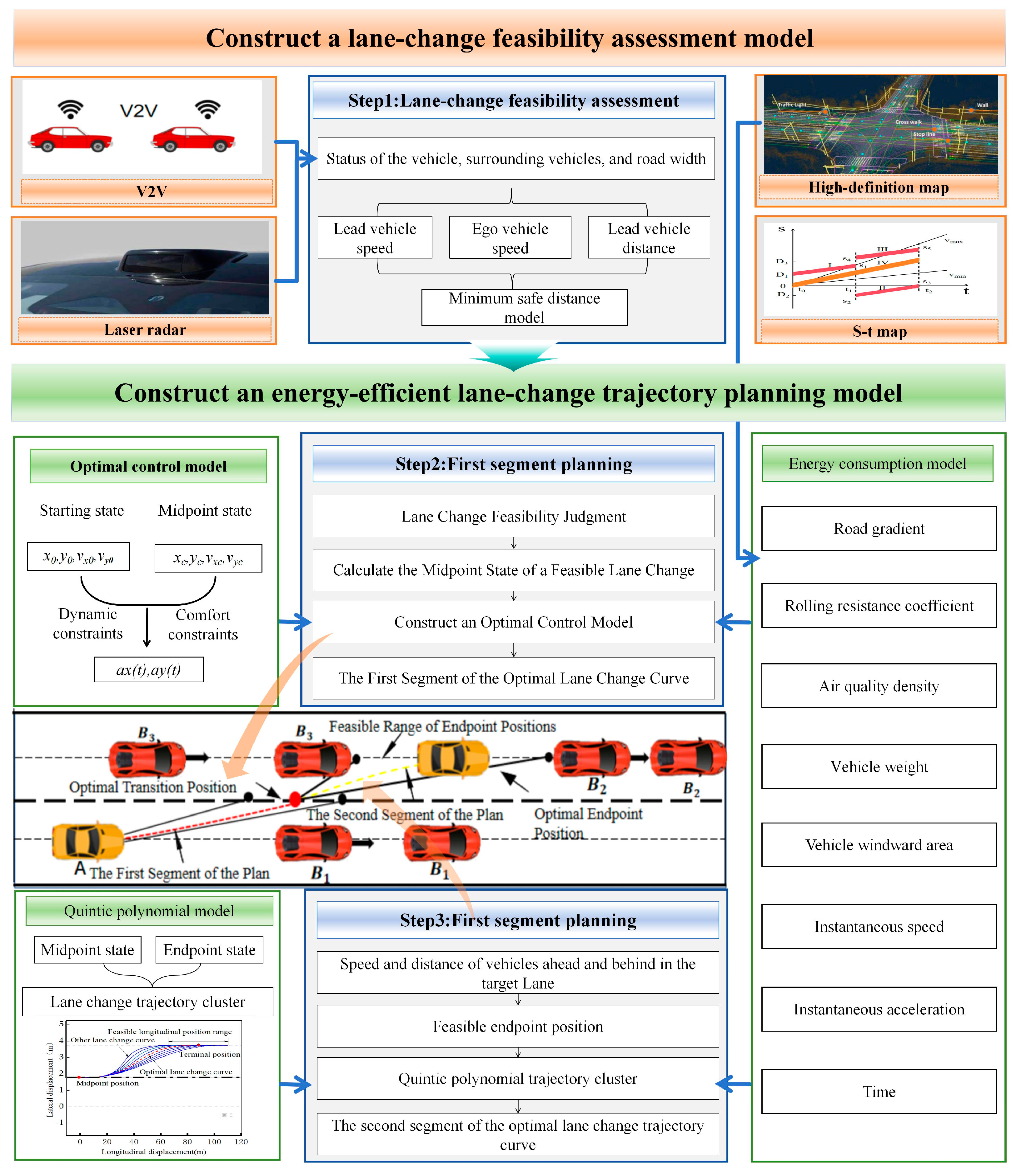
2. System Architecture

To achieve comfortable, safe, and economical lane changes, the complete lane-changing planning system is split into two primary modules: the lane-changing feasibility judgment module and the trajectory-planning module, as shown in Figure 1. The lane-changing feasibility assessment module takes into account obstacle vehicle information from both the present lane and the intended lane before initiating the lane change. It applies the minimum safe gap model [35] to assess whether a lane change is possible at the present moment. If a lane change is feasible, the system proceeds to the trajectory-planning module, where energy consumption optimization is set as a constraint, and the real-time lane-changing trajectories are planned in two segments using optimal control and quintic polynomials.

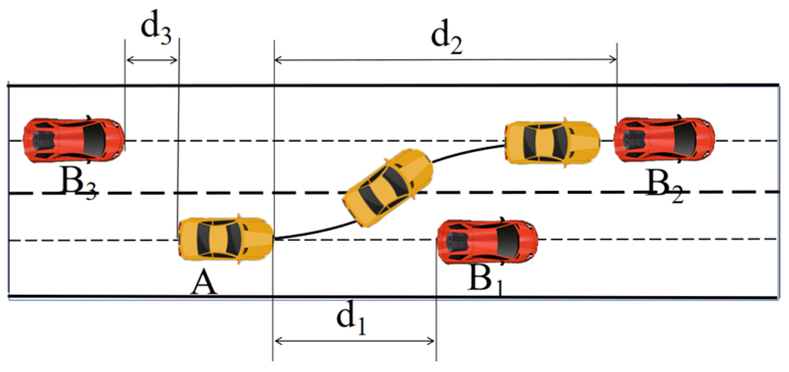
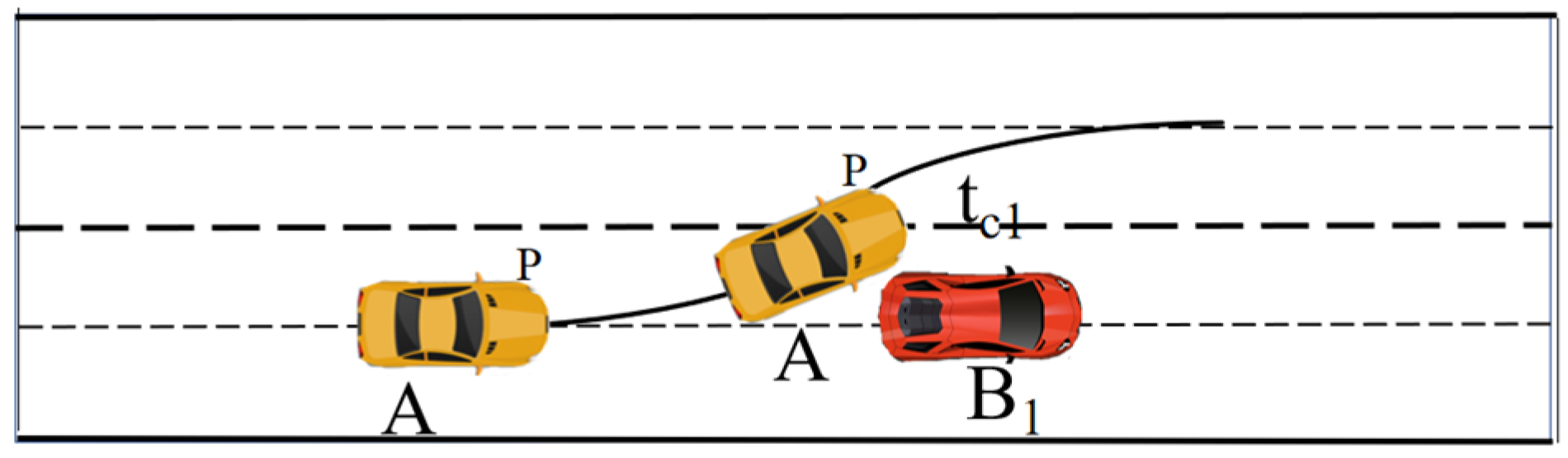
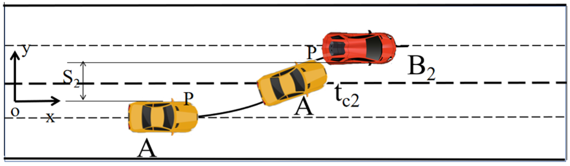
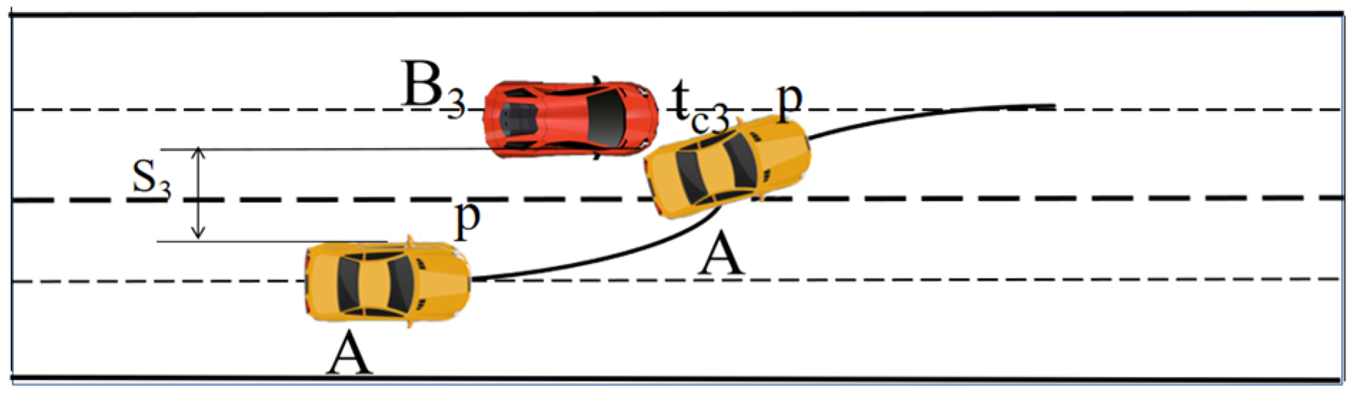
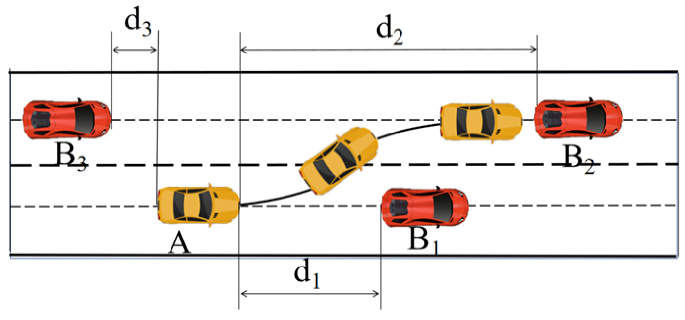
3. Lang-Changing Feasibility Modeling

Compared to the lower lane-changing speeds on urban roads, lane-changing on highways involves higher speeds and more significant energy consumption variations. Therefore, this study takes highway lane-change energy optimization as a representative example. The highway lane-changing scenario is illustrated in Figure 2. Before initiating the lane change, it is necessary to determine whether a safe lane change is feasible under current conditions based on information from surrounding vehicles. In this study, the minimum safety distance model is used to evaluate lane-change feasibility. The ego vehicle is denoted as A; B₁ represents the obstacle vehicle ahead in the current lane, while B₂ and B₃ represent the obstacle vehicles ahead of and behind the ego vehicle in the target lane, respectively. (For simplicity, all vehicles in this study are assumed to have a uniform width w = 1.8 m and length l = 4 m). The longitudinal velocity of the ego vehicle is v_A, and the longitudinal velocity and longitudinal acceleration of vehicle B_i are denoted by v_Bi and a_Bi, respectively. Let d₁ denote the initial longitudinal distance between vehicle A and B₁, d₂ is the initial longitudinal distance between A and the preceding vehicle B₂ in the target lane, and d₃ is the initial longitudinal distance between A and the following vehicle B₃ in the target lane. The parameter d₀ is used as a supplementary redundancy amount to buffer the potential risks from perception errors, vehicle response delays, and sudden state changes, typically set to 3 m [22]. Let t_c be the potential collision time between the ego vehicle and surrounding vehicles and t_f the final moment when the lane change is completed.

During the lane-changing process, the lateral acceleration and lateral velocity of all vehicles except the lane-changing vehicle are zero and move along the center line of the lane, and the lateral acceleration of the lane-changing vehicle can be expressed as a sinusoidal function of time t. The lateral velocity and lateral displacement can be expressed by integration as shown in Equation (1):

$$\begin{array}{l}{\mathrm{a}}_{\mathrm{l}\mathrm{a}\mathrm{t}}(\mathrm{t})={\displaystyle \frac{2\mathrm{\pi }\mathrm{H}}{{\mathrm{t}}_{\mathrm{f}}}}\times \sin ({\displaystyle \frac{2\mathrm{\pi }}{{\mathrm{t}}_{\mathrm{f}}}}\times \mathrm{t}),\forall \mathrm{t}\in \left[0,{\mathrm{t}}_{\mathrm{f}}\right]\\ {\mathrm{vy}}_{\mathrm{l}\mathrm{a}\mathrm{t}}(\mathrm{t})={\displaystyle {\int }_0^{\mathrm{t}}\frac{2\mathrm{\pi }\mathrm{H}}{{\mathrm{t}}_{\mathrm{f}}}\times \sin (\frac{2\mathrm{\pi }}{{\mathrm{t}}_{\mathrm{f}}}\times \mathrm{t})\mathrm{d}\mathrm{t}},\forall \mathrm{t}\in \left[0,{\mathrm{t}}_{\mathrm{f}}\right]\\ {\mathrm{y}}_{\mathrm{l}\mathrm{a}\mathrm{t}}(\mathrm{t})={\displaystyle {\int }_0^{\mathrm{t}}{\mathrm{vy}}_{\mathrm{l}\mathrm{a}\mathrm{t}}\mathrm{d}\mathrm{t}},\forall \mathrm{t}\in \left[0,{\mathrm{t}}_{\mathrm{f}}\right]\end{array}$$

(1)

In Equation (1), H denotes the lateral displacement of vehicle A during the entire lane-change process. Considering that in this study the ego vehicle A changes lanes from the centerline of the current lane to the centerline of the target lane, H is set to 3.75 m. The variable t_f represents the lane-change duration, typically ranging from 2 to 9 s [30], and it is set to 4 s in this study, following the relevant literature [35]. a_lat denotes the lateral acceleration during the lane-change process, vy_lat is the lateral velocity, and y_lat represents the lateral displacement throughout the maneuver.

(1) The minimum safety distance between the ego vehicle A and vehicle B₁

As shown in Figure 3, the ego vehicle A may collide with vehicle B₁ at time t_c1.

The collision time t_c1 can be obtained by solving the following Equation (2):

$${\mathrm{y}}_{\mathrm{l}\mathrm{a}\mathrm{t}}({\mathrm{t}}_{\mathrm{c}1})=\mathrm{w}\times \cos \mathrm{\theta }({\mathrm{t}}_{\mathrm{c}1})$$

(2)

In Equation (2), y_lat(t_c1) represents the lateral position of the front-left point of the ego vehicle A, w denotes the vehicle width, and θ is the heading angle.

The heading angle θ(t_c1) at this point can be calculated by the following Equation (3):

$$\mathrm{\theta }({\mathrm{t}}_{\mathrm{c}1})=\arctan {\displaystyle \frac{{\mathrm{v}}_{\mathrm{l}\mathrm{a}\mathrm{t}}({\mathrm{t}}_{\mathrm{c}1})}{{\mathrm{v}}_{\mathrm{a}}}}$$

(3)

The minimum safety distance between the ego vehicle A and vehicle B₁ can be calculated by the following Equation (4):

$$\mathrm{M}\mathrm{S}{\mathrm{S}}_{\mathrm{A},{\mathrm{B}}_1}=\max \left\{{\displaystyle {\int }_0^{\mathrm{t}}{\displaystyle {\int }_0^{\mathrm{\lambda }}\left[{\mathrm{a}}_{\mathrm{A}}(\mathrm{\tau })-{\mathrm{a}}_{{\mathrm{B}}_1}(\mathrm{\tau })\right]\mathrm{d}\mathrm{\tau }\mathrm{d}\mathrm{\lambda }+({\mathrm{v}}_{\mathrm{A}}(0)-{\mathrm{v}}_{{\mathrm{B}}_1}(0))\mathrm{t}}}\right\}\forall \mathrm{t}\in \left[0,{\mathrm{t}}_1\right]$$

(4)

To ensure that the ego vehicle A does not collide with vehicle B₁, the following condition must be satisfied:

$$\mathrm{M}\mathrm{S}{\mathrm{S}}_{\mathrm{A},{\mathrm{B}}_1}+{\mathrm{d}}_0<{\mathrm{d}}_1$$

(5)

(2) The minimum safety distance between the ego vehicle A and vehicle B₂

As shown in Figure 4, vehicle A may collide with vehicle B₂ at time t_c2. The collision time t_c2 can be obtained by solving the following Equation (6):

$${\mathrm{y}}_{\mathrm{l}\mathrm{a}\mathrm{t}}({\mathrm{t}}_{\mathrm{c}2})={\mathrm{S}}_2$$

(6)

In the equation, y_lat(t_c2) represents the lateral position of the front-left point P of the ego vehicle A, and S₂ denotes the initial lateral distance between the upper side of vehicle A and the lower side of obstacle vehicle B₂ at the starting moment. The value of S₂ can be calculated as 1.95 m.

The minimum safety distance between the ego vehicle A and obstacle vehicle B₂ can be calculated by the following Equation (7):

$$\mathrm{M}\mathrm{S}{\mathrm{S}}_{\mathrm{A},{\mathrm{B}}_2}=\max \left\{{\displaystyle {\int }_0^{\mathrm{t}}{\displaystyle {\int }_0^{\mathrm{\lambda }}\left[{\mathrm{a}}_{\mathrm{A}}(\mathrm{\tau })-{\mathrm{a}}_{{\mathrm{B}}_2}(\mathrm{\tau })\right]\mathrm{d}\mathrm{\tau }\mathrm{d}\mathrm{\lambda }+({\mathrm{v}}_{\mathrm{A}}(0)-{\mathrm{v}}_{{\mathrm{B}}_2}(0))\mathrm{t}}}\right\}\forall \mathrm{t}\in \left[{\mathrm{t}}_{\mathrm{c}2},{\mathrm{t}}_{\mathrm{f}}\right]$$

(7)

To ensure that the ego vehicle A does not collide with vehicle B₂, the following condition must be satisfied:

$$\mathrm{M}\mathrm{S}{\mathrm{S}}_{\mathrm{A},{\mathrm{B}}_2}+{\mathrm{d}}_0<{\mathrm{d}}_2$$

(8)

(3) The minimum safety distance between the ego vehicle A and vehicle B₃

As shown in Figure 5, the ego vehicle A may collide with vehicle B₃ at time t_c3.

The collision time t_c3 can be obtained by solving Equation (9):

$${\mathrm{y}}_{\mathrm{l}\mathrm{a}\mathrm{t}}({\mathrm{t}}_{\mathrm{c}3})-{\mathrm{l}}_{\mathrm{A}}\sin \mathrm{\theta }({\mathrm{t}}_{\mathrm{c}3})={\mathrm{S}}_3$$

(9)

In the equation, l_A represents the length of vehicle A, θ is the heading angle, y_lat(t_c3) is the lateral position of the front-left point P of vehicle A at time t_c3, and S₃ denotes the initial lateral distance between the upper side of vehicle A and the lower side of obstacle vehicle B₃ at the initial moment. The value of S₃ can be calculated as 1.95 m.

The heading angle θ(t_c3) of the vehicle at this point can be calculated by Equation (10):

$$\mathrm{\theta }({\mathrm{t}}_{\mathrm{c}3})=\arctan {\displaystyle \frac{{\mathrm{v}}_{\mathrm{l}\mathrm{a}\mathrm{t}}({\mathrm{t}}_{\mathrm{c}3})}{{\mathrm{v}}_{\mathrm{a}}}}$$

(10)

The minimum safe distance between ego vehicle A and obstacle vehicle B₃ can be calculated by Equation (11):

$$\mathrm{M}\mathrm{S}{\mathrm{S}}_{\mathrm{A},{\mathrm{B}}_3}=\max \left\{{\displaystyle {\int }_0^{\mathrm{t}}{\displaystyle {\int }_0^{\mathrm{\lambda }}\left[{\mathrm{a}}_{{\mathrm{B}}_3}(\mathrm{\tau })-{\mathrm{a}}_{\mathrm{A}}(\mathrm{\tau })\right]\mathrm{d}\mathrm{\tau }\mathrm{d}\mathrm{\lambda }+({\mathrm{v}}_{{\mathrm{B}}_3}(0)-{\mathrm{v}}_{\mathrm{A}}(0))\mathrm{t}}}\right\}\forall \mathrm{t}\in \left[{\mathrm{t}}_{\mathrm{c}3},{\mathrm{t}}_{\mathrm{f}}\right]$$

(11)

To ensure that ego vehicle A does not collide with vehicle B₃, the following condition must be satisfied:

$$\mathrm{M}\mathrm{S}{\mathrm{S}}_{\mathrm{A},{\mathrm{B}}_3}+{\mathrm{d}}_0<{\mathrm{d}}_3$$

(12)

4. Lane-Changing Trajectory-Planning Model

4.1. Lane-Changing Energy Consumption Cost Function

Ding et al. [36] showed that the frequency of lane changing increases when a vehicle is traveling in a regular-state traffic flow compared to a free-state traffic flow, which in turn leads to an increase in the overall driving energy consumption by about 8%. Meanwhile, Mehlig et al. [37] and Zhao et al. [38] show that the rapid development of electric vehicles will help to change the environmental impact of road transportation, so the energy-saving optimization of the lane-change process of intelligent electric vehicles can enhance the energy efficiency of individual vehicles but also help to improve traffic mobility at the macro level and accelerate the popularization of electric vehicles.

Compared to traditional gasoline vehicles, electric vehicles (EVs) are equipped with regenerative braking systems that can recover energy during braking. As a result, their energy consumption models are more complex than those of gasoline-powered vehicles. In this study, we adopt the VT-CPEM energy consumption model proposed in [39], which takes inputs such as road gradient, vehicle acceleration, and speed to evaluate the energy consumption of an electric vehicle over a specific driving cycle. During normal driving, the electric motor powers the wheels. However, when the brake pedal is pressed or the accelerator is released, the motor switches to generator mode. The wheels, driven by inertia, cause the motor to rotate in reverse, converting mechanical energy into electrical energy. This recovered energy is then stored in the battery system, thereby improving the overall energy efficiency of the vehicle. In the VT-CPEM model, the efficiency of regenerative braking is modeled as a function of vehicle deceleration, rather than being treated as a fixed value or as dependent solely on vehicle speed, as in traditional models. This approach more accurately captures the dynamic characteristics of energy recovery during real-world driving conditions.

Considering the air resistance, rolling resistance, road gradient, and inertial forces during the electric vehicle’s motion, the power at the wheels can be expressed as P_Wheels(t):

$$\begin{array}{l}{\mathrm{P}}_{\mathrm{W}\mathrm{h}\mathrm{e}\mathrm{e}\mathrm{l}\mathrm{s}}\left(\mathrm{t}\right)=((\mathrm{m}\mathrm{a}(\mathrm{t})+\mathrm{m}\mathrm{g}\cdot \cos (\mathrm{\alpha })\cdot {\displaystyle \frac{{\mathrm{C}}_{\mathrm{r}}}{1000}}({\mathrm{c}}_1\mathrm{v}(\mathrm{t})+{\mathrm{c}}_2)+\\ \hfill {\displaystyle \frac{1}{2}}{\mathrm{\rho }}_{\mathrm{Air}}{\mathrm{A}}_{\mathrm{f}}{\mathrm{C}}_{\mathrm{D}}{\mathrm{v}}^2(\mathrm{t})+\mathrm{m}\mathrm{g}\cdot \sin (\mathrm{\alpha }))\cdot \mathrm{v}(\mathrm{t})\end{array}$$

(13)

In Equation (3), v(t) represents the vehicle’s speed, a(t) indicates the vehicle’s acceleration (negative during deceleration), g is the gravitational acceleration, and α refers to the road gradient. C_r = 1.75, C₁ = 0.0328, and C₂ = 4.575 represent the rolling resistance parameters [39], which vary with road surface conditions. m denotes the vehicle’s mass, t represents the driving time, P_Air = 1.25536 stands for the air density, A_f refers to the vehicle’s frontal area, and C_D = 0.28 refers to the aerodynamic drag coefficient.

This model accounts for the various forces acting on the vehicle while driving, including air resistance, rolling resistance, gravitational forces, and inertia, to estimate the energy consumption throughout the lane-changing process.

$$\left\{\begin{array}{l}{\mathrm{E}}_{\mathrm{C}\mathrm{o}\mathrm{n}\mathrm{s}\mathrm{u}\mathrm{m}\mathrm{e}}(\mathrm{v}(\mathrm{t}),\mathrm{a}(\mathrm{t}))={\displaystyle {\int }_0^{\mathrm{t}}{\mathrm{P}}_{\mathrm{W}\mathrm{h}\mathrm{e}\mathrm{e}\mathrm{l}\mathrm{s}}\left(\mathrm{v}(\mathrm{t}),\mathrm{a}(\mathrm{t})\right)}\mathrm{d}\mathrm{t},\mathrm{a}(\mathrm{t})>0\\ {\mathrm{E}}_{\mathrm{R}\mathrm{e}\mathrm{c}\mathrm{o}\mathrm{v}\mathrm{e}\mathrm{r}\mathrm{a}\mathrm{b}\mathrm{l}\mathrm{e}}(\mathrm{v}(\mathrm{t}),\mathrm{a}(\mathrm{t}))={\displaystyle {\int }_0^{\mathrm{t}}{\mathrm{P}}_{\mathrm{W}\mathrm{h}\mathrm{e}\mathrm{e}\mathrm{l}\mathrm{s}}^{(-)}\left(\mathrm{v}(\mathrm{t}),\mathrm{a}(\mathrm{t})\right)}\mathrm{d}\mathrm{t}\times {\mathrm{\eta }}_{\mathrm{r}\mathrm{b}},\mathrm{a}(\mathrm{t})<0\end{array}\right.$$

(14)

$${\mathrm{\eta }}_{\mathrm{r}\mathrm{b}}(\mathrm{t})={\left[{\mathrm{e}}^{\left({\displaystyle \frac{0.041}{|\mathrm{a}(\mathrm{t})|}}\right)}\right]}^{-1}$$

(15)

In Equation (14), E_Consume denotes the consumed energy, E_Recoverable denotes the recovered energy, and η_rb is the efficiency of regenerative braking.

Thus, the cost function E can be established as shown in Equation (16):

$$\mathrm{E}(\mathrm{v}(\mathrm{t}),\mathrm{a}(\mathrm{t}))={\mathrm{E}}_{\mathrm{C}\mathrm{o}\mathrm{n}\mathrm{s}\mathrm{u}\mathrm{m}\mathrm{e}}(\mathrm{v}(\mathrm{t}),\mathrm{a}(\mathrm{t}))-{\mathrm{E}}_{\mathrm{R}\mathrm{e}\mathrm{cov}\mathrm{e}\mathrm{r}\mathrm{a}\mathrm{b}\mathrm{l}\mathrm{e}}(\mathrm{v}(\mathrm{t}),\mathrm{a}(\mathrm{t}))$$

(16)

4.2. Optimal Control Combined with Quintic Polynomial for Piecewise Trajectory Planning

This study proposes a real-time planning method that combines optimal control with quintic polynomials. Given the advantages of optimal control and quintic polynomials in terms of energy optimization and computational speed, the method uses optimal control for the first segment of the trajectory planning and quintic polynomials for the second segment. The approach first solves for the optimal intermediate state and then plans the first segment of the lane-change trajectory. Upon reaching the midpoint, the speed of the surrounding vehicles in the target lane, as well as their distances from the ego vehicle, are used to calculate a suitable endpoint range. Next, a quintic polynomial is used to design the second segment of the lane-changing trajectory. This approach results in a path with a low computational complexity, offering excellent real-time performance. Through the two-step planning process, the lane-changing trajectory can be adjusted dynamically.

4.2.1. First-Segment Trajectory Planning

The process from the starting point to the midpoint is shown in Figure 6. It is assumed that all vehicles are traveling along the lane’s centerline. As the lane change starts, the ego vehicle A’s longitudinal velocity is denoted as v_x0, the lateral velocity v_y0 is 0, and the longitudinal velocity of the obstacle vehicle B₁ ahead of the ego vehicle is v_B1.The initial longitudinal separation between the two vehicles is symbolized as d_s. The starting state of the ego vehicle at the initiation of the lane change is (0, 0, v_x0, 0), and the state at the midpoint of the lane change is (s_xc, s_yc, v_xc, v_yc). Since the yaw angle of the vehicle during the lane change process is very small, the yaw angle of the vehicle at the midpoint is ignored, meaning the vehicle is assumed to be parallel to the lane at the midpoint. Considering that there should be no lateral interference with the preceding vehicle in the target lane at the midpoint of the lane change, the lateral position s_yc is set to 1.8 m, which is slightly greater than the width of the obstacle vehicle. (In this study, all vehicles are assumed to have a width of 1.7 m and a length of 4 m.). To generate a feasible longitudinal safe region, it is assumed that the ego vehicle A accelerates uniformly with the maximum allowable longitudinal acceleration of 2 m/s². For the obstacle vehicle B₁ ahead, it is assumed to decelerate uniformly. As shown in Figure 7, in the 4880 datasets obtained from the highD dataset. [40], the maximum longitudinal acceleration of drivers is generally between −2 m/s² and 2 m/s². Therefore, the deceleration of the obstacle vehicle B₁ is set to −2 m/s².

Therefore, the velocity range of the ego vehicle A at the midpoint of the lane change can be calculated. Denote the maximum time allowed for lane changing in the first segment of trajectory planning as t₁. When the ego vehicle A reaches the midpoint, its longitudinal velocity is v_xc, and its lateral velocity is v_yc. Considering that in practical lane-change processes, vehicles typically accelerate first, if the ego vehicle A accelerates uniformly, its maximum longitudinal velocity at the midpoint can reach v_x0 + 2t₁. Therefore, the longitudinal velocity at the midpoint satisfies v_xc ∈ [v_x0, v_x0 + 2t₁]. According to the highD dataset (as shown in Figure 4), drivers’ lateral velocity generally does not exceed 2 m/s. Hence, based on real driver behavior, this study sets the lateral velocity range at the midpoint as v_yc ∈ [0, 2]; considering the optimal control problem solution time is about 0.05 s (derived from the simulation verification in the third part of the article), to eliminate the error introduced by the solution time, the actual distance d₁ between the front obstacle vehicle B₁ and the ego vehicle A at the start of the first lane change process is shown in Equation (17).

d₁ = d_s − (v_x0 − v_B1) × 0.05

(17)

The maximum longitudinal displacement x_A1 of the ego vehicle A during the process from the starting point to the midpoint position is shown in Equation (18).

$${\mathrm{x}}_{\mathrm{A}1}={\displaystyle {\int }_0^{{\mathrm{t}}_1}{\displaystyle {\int }_0^{\mathrm{\lambda }}{\mathrm{a}}_{\mathrm{A}1}}}\mathrm{d}\mathrm{\tau }\mathrm{d}\mathrm{\lambda }+{\mathrm{v}}_{\mathrm{x}0}{\mathrm{t}}_1$$

(18)

x_A1 represents the maximum longitudinal displacement of the ego vehicle A during the process from the starting point to the midpoint position; a_A1 the maximum longitudinal acceleration of the ego vehicle A (set to 2 m/s²); v_x0 is the initial longitudinal velocity of the ego vehicle A; and t₁ is the maximum allowable lane-change time for vehicle A to travel from the starting point to the midpoint position.

During the process in which the ego vehicle A moves from the starting point to the midpoint position, the minimum longitudinal displacement x_B1 of vehicle B₁ is shown in Equation (19).

$${\mathrm{x}}_{\mathrm{B}1}={\displaystyle {\int }_0^{{\mathrm{t}}_1}{\displaystyle {\int }_0^{\mathrm{\lambda }}{\mathrm{a}}_{\mathrm{B}1}}}\mathrm{d}\mathrm{\tau }\mathrm{d}\mathrm{\lambda }+{\mathrm{v}}_{\mathrm{B}1}{\mathrm{t}}_1$$

(19)

In addition, a_B1 is the maximum longitudinal deceleration of vehicle B₁ (set to –2 m/s²); and v_B1 represents the initial longitudinal velocity of vehicle B₁.

To avoid longitudinal collision during the initial lane change, the following conditions need to be satisfied as shown in Equation (20).

$${\mathrm{d}}_1+{\mathrm{x}}_{\mathrm{B}1}>{\mathrm{x}}_{\mathrm{A}1}$$

(20)

With Equation (20), we can inverse-solve for the maximum permissible changeover time and the actual changeover time t_c ∈ [0, t₁] and bring t_c into Equation (18), at which point we can determine the range of the states of the midpoint of the changeover to be (s_xc ∈ [0, ${\displaystyle {\int }_0^{{\mathrm{t}}_{\mathrm{c}}}{\displaystyle {\int }_0^{\mathrm{\lambda }}{\mathrm{a}}_{\mathrm{A}}}}\mathrm{d}\mathrm{\tau }\mathrm{d}\mathrm{\lambda }+{\mathrm{v}}_{\mathrm{x}0}{\mathrm{t}}_{\mathrm{c}}$], s_yc = 1.8, v_xc ∈ [v₀, v₀ + 2t_c], v_yc ∈ [0, 2]).

4.2.2. Optimal Control Solves for the First Segment of the Lane-Change Trajectory

The optimal lane-change transit position, as well as the optimal trajectory, are solved by constructing the optimal control. The state vectors are transverse displacement, longitudinal displacement, transverse velocity, and longitudinal velocity during lane changing as shown in Equation (21).

$$\mathrm{X}(\mathrm{t})={\left[{\mathrm{x}}_1(\mathrm{t}),{\mathrm{x}}_2(\mathrm{t}),{\mathrm{x}}_3(\mathrm{t}),{\mathrm{x}}_4(\mathrm{t})\right]}^{\mathrm{T}}={\left[{\mathrm{s}}_{\mathrm{x}}(\mathrm{t}),{\mathrm{s}}_{\mathrm{y}}(\mathrm{t}),{\mathrm{v}}_{\mathrm{x}}(\mathrm{t}),{\mathrm{v}}_{\mathrm{y}}(\mathrm{t})\right]}^{\mathrm{T}}$$

(21)

s_x(t) denotes the longitudinal displacement of the ego vehicle, s_y(t) denotes the lateral displacement, and v_x(t) and v_y(t) represent the longitudinal and lateral velocities, respectively. x₁(t), x₂(t), x₃(t), and x₄(t) constitute the state vector.

The control vectors are lateral acceleration and longitudinal acceleration as shown in Equation (22).

$$\mathrm{u}(\mathrm{t})={[{\mathrm{u}}_1(\mathrm{t}),{\mathrm{u}}_2(\mathrm{t})]}^{\mathrm{T}}={[{\mathrm{a}}_{\mathrm{x}}(\mathrm{t}),{\mathrm{a}}_{\mathrm{y}}(\mathrm{t})]}^{\mathrm{T}}$$

(22)

a_x(t) is the longitudinal acceleration, and a_y(t) is the lateral acceleration. u₁(t), u₂(t) are the control vectors

The continuous state space is discretized over time, and γ is a differential unit as shown in Equation (23):

$$\begin{array}{l}{\mathrm{t}}_0\le \mathrm{k}\mathrm{\gamma }\le {\mathrm{t}}_{\mathrm{c}}, {\mathrm{t}}_0={\mathrm{k}}_0\mathrm{\gamma } ,{\mathrm{t}}_{\mathrm{c}}={\mathrm{k}}_{\mathrm{c}}\mathrm{\gamma }\\ \left\{\begin{array}{l}{\mathrm{v}}_{\mathrm{x}}(\mathrm{k})={\mathrm{v}}_{\mathrm{x}}({\mathrm{k}}_0)+{\displaystyle \sum _{\mathrm{i}={\mathrm{k}}_0}^{\mathrm{k}-1}{\mathrm{a}}_{\mathrm{x}}(\mathrm{i})}\mathrm{\gamma }\\ {\mathrm{v}}_{\mathrm{y}}(\mathrm{k})={\mathrm{v}}_{\mathrm{y}}({\mathrm{k}}_0)+{\displaystyle \sum _{\mathrm{i}={\mathrm{k}}_0}^{\mathrm{k}-1}{\mathrm{a}}_{\mathrm{y}}(\mathrm{i})}\mathrm{\gamma }\\ {\mathrm{s}}_{\mathrm{x}}(\mathrm{k})={\mathrm{s}}_{\mathrm{x}}({\mathrm{k}}_0)+(\mathrm{k}-{\mathrm{k}}_0){\mathrm{v}}_{\mathrm{x}}({\mathrm{k}}_0)\mathrm{\gamma }+{\mathrm{\gamma }}^2{\displaystyle \sum _{\mathrm{i}={\mathrm{k}}_0}^{\mathrm{k}-1}\mathrm{k}-\mathrm{i}-\frac{1}{2}{\mathrm{a}}_{\mathrm{x}}(\mathrm{i})}\\ {\mathrm{s}}_{\mathrm{y}}(\mathrm{k})={\mathrm{s}}_{\mathrm{y}}({\mathrm{k}}_0)+(\mathrm{k}-{\mathrm{k}}_0){\mathrm{v}}_{\mathrm{y}}({\mathrm{k}}_0)\mathrm{\gamma }+{\mathrm{\gamma }}^2{\displaystyle \sum _{\mathrm{i}={\mathrm{k}}_0}^{\mathrm{k}-1}\mathrm{k}-\mathrm{i}-\frac{1}{2}{\mathrm{a}}_{\mathrm{y}}(\mathrm{i})}\end{array}\right.\end{array}$$

(23)

The vehicle kinematic constraints are shown in Equation (24).

$$\dot{\mathrm{x}}(\mathrm{t})\triangleq \left[\begin{array}{c}{\dot{\mathrm{x}}}_1(\mathrm{t})={\mathrm{v}}_{\mathrm{x}}(\mathrm{t})={\displaystyle \frac{{\mathrm{s}}_{\mathrm{x}}(\mathrm{k}+1)-{\mathrm{s}}_{\mathrm{x}}(\mathrm{k})}{\mathrm{\gamma }}}\\ {\dot{\mathrm{x}}}_2(\mathrm{t})={\mathrm{v}}_{\mathrm{y}}(\mathrm{t})={\displaystyle \frac{{\mathrm{s}}_{\mathrm{y}}(\mathrm{k}+1)-{\mathrm{s}}_{\mathrm{y}}(\mathrm{k})}{\mathrm{\gamma }}}\\ {\dot{\mathrm{x}}}_3(\mathrm{t})={\mathrm{a}}_{\mathrm{x}}(\mathrm{t})={\displaystyle \frac{{\mathrm{v}}_{\mathrm{x}}(\mathrm{k}+1)-{\mathrm{v}}_{\mathrm{x}}(\mathrm{k})}{\mathrm{\gamma }}}\\ {\dot{\mathrm{x}}}_4(\mathrm{t})={\mathrm{a}}_{\mathrm{y}}(\mathrm{t})={\displaystyle \frac{{\mathrm{v}}_{\mathrm{y}}(\mathrm{k}+1)-{\mathrm{v}}_{\mathrm{y}}(\mathrm{k})}{\mathrm{\gamma }}}\end{array}\right]$$

(24)

Considering the impact of lane-changing operations on passenger comfort, this study primarily relates comfort to the lateral acceleration during lane changes. For motion-sensitive passengers, the comfort threshold of the maximum acceptable lateral acceleration is 0.203 g [41]. Other factors, such as the vehicle’s maximum steering angle, are also considered. The corresponding constraints are shown in Equation (25).

$$\left\{\begin{array}{l}-2\le {\mathrm{a}}_{\mathrm{x}}(\mathrm{t})\le 2\\ -2\le {\mathrm{a}}_{\mathrm{y}}(\mathrm{t})\le 2\\ {\mathrm{v}}_{\mathrm{x}\min }\le {\mathrm{v}}_{\mathrm{x}}(\mathrm{t})\le {\mathrm{v}}_{\mathrm{x}\max }\\ {\mathrm{v}}_{\mathrm{y}\min }\le {\mathrm{v}}_{\mathrm{y}}(\mathrm{t})\le {\mathrm{v}}_{\mathrm{y}\max }\\ 0\le \mathrm{\theta }(\mathrm{t})=\arctan {\displaystyle \frac{{\mathrm{a}}_{\mathrm{y}}(\mathrm{t})}{{\mathrm{a}}_{\mathrm{x}}(\mathrm{t})}}\le {45}^{\circ }\end{array}\right.$$

(25)

v_xmax is the maximum permissible longitudinal velocity at high velocity (33.33 m/s), and v_xmin is the minimum longitudinal velocity at high velocity (16.67 m/s). v_ymax is the maximum lateral velocity for passenger comfort (2 m/s), and v_ymin is the minimum lateral velocity for passenger comfort (−2 m/s). θ(t) is the heading angle.

The initial state of channel change is shown in Equation (26).

$$\mathrm{X}(\mathrm{t}=0)={\left[{\mathrm{s}}_{\mathrm{x}0},{\mathrm{s}}_{\mathrm{y}0},{\mathrm{v}}_{\mathrm{x}0},{\mathrm{v}}_{\mathrm{y}0}\right]}^{\mathrm{T}}={\left[0,0,{\mathrm{v}}_{\mathrm{x}0},0\right]}^{\mathrm{T}}$$

(26)

s_x0, s_y0 are the position coordinates at the start of the lane change, and v_x0, v_y0 are the longitudinal and lateral velocities at the start of the lane change.

The lane change transit state is shown in Equation (27).

$$\mathrm{X}(\mathrm{t}={\mathrm{t}}_{\mathrm{c}})={\left[{\mathrm{s}}_{\mathrm{x}\mathrm{c}},{\mathrm{s}}_{\mathrm{y}\mathrm{c}},{\mathrm{v}}_{\mathrm{x}\mathrm{c}},{\mathrm{v}}_{\mathrm{y}\mathrm{c}}\right]}^{\mathrm{T}}={\left[[0,{\mathrm{X}}_{\mathrm{A}1}],1.8,[{\mathrm{v}}_{\mathrm{x}0},{\mathrm{v}}_{\mathrm{x}0}+2{\mathrm{t}}_{\mathrm{c}}],[0,2]\right]}^{\mathrm{T}}$$

(27)

s_xc, s_yc are the coordinates of the transit position of the lane change, and v_xc, v_yc are the transverse and longitudinal velocities at the transit position.

Constructing the cost function considering comfort, efficiency, and energy consumption is shown in Equation (28).

$$\begin{array}{l}\left\{\begin{array}{l}\mathrm{E}(\mathrm{v}(\mathrm{t}),\mathrm{a}(\mathrm{t}))=\mathrm{m}\mathrm{i}\mathrm{n}({\mathrm{E}}_{\mathrm{C}\mathrm{o}\mathrm{n}\mathrm{s}\mathrm{u}\mathrm{m}\mathrm{e}}(\mathrm{v}(\mathrm{t}),\mathrm{a}(\mathrm{t}))-{\mathrm{E}}_{\mathrm{R}\mathrm{e}\mathrm{c}\mathrm{o}\mathrm{v}\mathrm{e}\mathrm{r}\mathrm{a}\mathrm{b}\mathrm{l}\mathrm{e}}(\mathrm{v}(\mathrm{t}),\mathrm{a}(\mathrm{t})))\\ \mathrm{v}(\mathrm{t})=\sqrt{{\mathrm{v}}_{\mathrm{x}}{(\mathrm{t})}^2+{\mathrm{v}}_{\mathrm{y}}{(\mathrm{t})}^2}\\ \mathrm{a}(\mathrm{t})=\sqrt{{\mathrm{a}}_{\mathrm{x}}{(\mathrm{t})}^2+{\mathrm{a}}_{\mathrm{y}}{(\mathrm{t})}^2}\end{array}\right.\\ \min \mathrm{J}={\mathrm{\beta }}_1\times {\displaystyle \frac{{\displaystyle {\int }_0^{{\mathrm{t}}_{\mathrm{c}}}{\left(\ddot{\mathrm{y}}(\mathrm{t})\right)}^2}\mathrm{d}\mathrm{t}}{{\displaystyle {\int }_0^{{\mathrm{t}}_{\mathrm{c}}}{\left({\mathrm{a}}_{\mathrm{ymax}}\right)}^2\mathrm{d}\mathrm{t}}}}+{\mathrm{\beta }}_2\times {\displaystyle \frac{{\mathrm{t}}_{\mathrm{c}}}{{\mathrm{t}}_{\mathrm{m}\mathrm{a}\mathrm{x}}}}+{\mathrm{\beta }}_3\times {\displaystyle \frac{\mathrm{E}(\mathrm{v}(\mathrm{t}),\mathrm{a}(\mathrm{t}))}{{\mathrm{E}}_{\mathrm{m}\mathrm{a}\mathrm{x}}}},\\ {\mathrm{\beta }}_1+{\mathrm{\beta }}_2+{\mathrm{\beta }}_3=1\end{array}$$

(28)

where β₁, β₂, β₃ are the weighting coefficients; a_ymax is 2; t_max is taken as 4 s; and E_max can be calculated based on the maximum duration of the lane change and the final speed at the end of the maneuver. For different driving environments and driving styles, the weighting factor can be adjusted, and in this study energy consumption is used as the optimal purpose, so β₃ is set to 0.8, β₁ is set to 0.1, and β₂ is set to 0.1. J is the cost function.

The optimal control model can be solved using the commercial software GPOPSⅡ Version 2.1 to obtain the optimal lane-change trajectory.

4.2.3. Second-Segment Trajectory Planning

When the ego vehicle arrives at the staging position, the second planning segment begins. Since the computation time for quintic polynomial planning is only about 2 ms, the time effect can be ignored. Assuming that there are two obstacle vehicles B₂ and B₃ in front and behind the target lane at this moment, with the lane-changing process illustrated in Figure 8, firstly, consider the leading vehicle B₂ in the target lane; at this time, the distance between the front end of vehicle A and the rear end of vehicle B₂ is denoted as d₂, and the speed of the front vehicle B₂ is v_B2. Referring to the modeling method of the first planning segment, also, to ensure no collision with the leading vehicle, this time it can be assumed that the ego vehicle is accelerating in the second lane-changing procedure, and it will accelerate uniformly at the maximum allowable acceleration, to determine the maximum longitudinal displacement of the ego vehicle and the acceleration, as well as to identify the maximum longitudinal displacement from the ego vehicle.

The maximum longitudinal displacement x_A2 of the ego vehicle during the second lane change is shown in Equation (29).

$${\mathrm{x}}_{\mathrm{A}2}={\displaystyle {\int }_0^{{\mathrm{t}}_2}{\displaystyle {\int }_0^{\mathrm{\lambda }}{\mathrm{a}}_{\mathrm{A}2}}}\mathrm{d}\mathrm{\tau }\mathrm{d}\mathrm{\lambda }+{\mathrm{v}}_{\mathrm{x}\mathrm{c}}{\mathrm{t}}_2$$

(29)

a_A2 denotes the maximum longitudinal acceleration of the ego vehicle A, which is set to 2 m/s². t₂ is the maximum allowable lane-change time for ego vehicle A to avoid interference with vehicle B₂ from the midpoint to the endpoint.

The preceding vehicle in the target lane slows down at a maximum longitudinal deceleration rate a_B2 of −2 m/s², and the minimum longitudinal displacement is shown in Equation (30).

$${\mathrm{x}}_{\mathrm{B}2}={\displaystyle {\int }_0^{{\mathrm{t}}_2}{\displaystyle {\int }_0^{\mathrm{\lambda }}{\mathrm{a}}_{\mathrm{B}2}}}\mathrm{d}\mathrm{\tau }\mathrm{d}\mathrm{\lambda }+{\mathrm{v}}_{\mathrm{B}2}{\mathrm{t}}_2$$

(30)

To prevent a collision with obstacle vehicle B₂ during the lane change, the following conditions need to be satisfied as shown in Equation (31).

$${\mathrm{d}}_2+{\mathrm{x}}_{\mathrm{B}2}>{\mathrm{x}}_{\mathrm{A}2}$$

(31)

From this, the maximum permissible lane-change time t₂ can be calculated. At the beginning of the second planning segment, the velocity of the following vehicle B₃ in the target lane is denoted as v_B3, and the longitudinal distance between the front end of B₃ and the rear end of the ego vehicle A is d₃. To avoid a rear-end collision, it is assumed that vehicle B₃ accelerates during the lane-changing process, while the ego vehicle decelerates uniformly. The minimum longitudinal displacement of the ego vehicle is given in Equation (32).

$${\mathrm{x}}_{\mathrm{A}3}={\displaystyle {\int }_0^{{\mathrm{t}}_3}{\displaystyle {\int }_0^{\mathrm{\lambda }}{\mathrm{a}}_{\mathrm{A}}}}\mathrm{d}\mathrm{\tau }\mathrm{d}\mathrm{\lambda }+{\mathrm{v}}_{\mathrm{x}\mathrm{c}}{\mathrm{t}}_3$$

(32)

The maximum longitudinal displacement of the rear vehicle is as shown in Equation (33).

$${\mathrm{x}}_{\mathrm{B}3}={\displaystyle {\int }_0^{{\mathrm{t}}_3}{\displaystyle {\int }_0^{\mathrm{\lambda }}{\mathrm{a}}_{\mathrm{B}3}}}\mathrm{d}\mathrm{\tau }\mathrm{d}\mathrm{\lambda }+{\mathrm{v}}_{\mathrm{B}3}{\mathrm{t}}_3$$

(33)

t₃ is the maximum permissible lane-change time for ego vehicle A to avoid interference with vehicle B₃ from the midpoint to the endpoint

To ensure no collision with the trailing obstacle vehicle in the longitudinal displacement during the lane change, the following condition is satisfied as shown in Equation (34).

$${\mathrm{d}}_3+{\mathrm{x}}_{\mathrm{A}3}>{\mathrm{x}}_{\mathrm{B}3}$$

(34)

From this, we can calculate the maximum lane change time t₃ allowed at this point, and the actual maximum lane change time t_e ∈ [0, min(t₃, t₂)] for the second planning segment. Eventually, we can obtain the range of the terminal state as (s_xe ∈ [${\displaystyle {\int }_0^{{\mathrm{t}}_3}{\displaystyle {\int }_0^{\mathrm{\lambda }}{\mathrm{a}}_{\mathrm{A}}}}\mathrm{d}\mathrm{\tau }\mathrm{d}\mathrm{\lambda }+{\mathrm{v}}_{\mathrm{x}\mathrm{c}}{\mathrm{t}}_3$, ${\displaystyle {\int }_0^{{\mathrm{t}}_2}{\displaystyle {\int }_0^{\mathrm{\lambda }}{\mathrm{a}}_{\mathrm{A}}}}\mathrm{d}\mathrm{\tau }\mathrm{d}\mathrm{\lambda }+{\mathrm{v}}_{\mathrm{x}\mathrm{c}}{\mathrm{t}}_2$], 3.75, v_xe, 0), v_xe is the desired target speed, and the end of the lane change is required to be 0 for the lateral acceleration and the longitudinal acceleration; the state of the terminal position is (s_xe, 3.75, v_xe, 0, 0, 0), and the state of the midpoint is obtained in the first segment of the planning as (s_xe, 1.8, v_xc, v_yc, a_xc, a_yc). Then in steps of 1 s, the range of t_e is first discretized as (t_e1, t_e2, …, t_eN), N being the number of t_e discrete points, and at each t_ei moment in steps of 5 m, we discretize the range of s_xe as (s_xe1, s_xe2, …, s_xeM), M being the number of s_xe discrete points.

4.2.4. Quintic Polynomial Programming to Solve for the Second Segment of Lane-Change Trajectories

The vehicle trajectory is represented as a function of time t in both the lateral and longitudinal directions, as shown in Equation (35).

$$\left\{\begin{array}{l}\mathrm{x}{(\mathrm{t})}_{\mathrm{m}\times \mathrm{n}}={\mathrm{a}}_{0\mathrm{m}\times \mathrm{n}}+{\mathrm{a}}_{1\mathrm{m}\times \mathrm{n}}\mathrm{t}+{\mathrm{a}}_{2\mathrm{m}\times \mathrm{n}}{\mathrm{t}}^2+{\mathrm{a}}_{3\mathrm{m}\times \mathrm{n}}{\mathrm{t}}^3+{\mathrm{a}}_{4\mathrm{m}\times \mathrm{n}}{\mathrm{t}}^4+{\mathrm{a}}_{5\mathrm{m}\times \mathrm{n}}{\mathrm{t}}^5\hspace{1em}\mathrm{m}=1,2,\cdots ,\mathrm{M};,\mathrm{n}=1,2,\cdots ,\mathrm{N}\\ \mathrm{y}{(\mathrm{t})}_{\mathrm{m}\times \mathrm{n}}={\mathrm{b}}_{0\mathrm{m}\times \mathrm{n}}+{\mathrm{b}}_{1\mathrm{m}\times \mathrm{n}}\mathrm{t}+{\mathrm{b}}_{2\mathrm{m}\times \mathrm{n}}{\mathrm{t}}^2+{\mathrm{b}}_{3\mathrm{m}\times \mathrm{n}}{\mathrm{t}}^3+{\mathrm{b}}_{4\mathrm{m}\times \mathrm{n}}{\mathrm{t}}^4+{\mathrm{b}}_{5\mathrm{m}\times \mathrm{n}}{\mathrm{t}}^5\end{array}\right.$$

(35)

The lane-change transit state is shown in Equation (36).

$$\left\{\begin{array}{ll}\mathrm{x}(\mathrm{t}={\mathrm{t}}_{\mathrm{c}})={\mathrm{s}}_{\mathrm{x}\mathrm{c}}\hfill & \hspace{1em}\mathrm{y}(\mathrm{t}={\mathrm{t}}_{\mathrm{c}})=1.8\hfill \\ \dot{\mathrm{x}}(\mathrm{t}={\mathrm{t}}_{\mathrm{c}})=\mathrm{\nu }{\mathrm{x}}_{\mathrm{c}}\hfill & \hspace{1em}\dot{\mathrm{y}}(\mathrm{t}={\mathrm{t}}_{\mathrm{c}})=\mathrm{v}{\mathrm{y}}_{\mathrm{c}}\hfill \\ \ddot{\mathrm{x}}(\mathrm{t}={\mathrm{t}}_{\mathrm{c}})=\mathrm{a}{\mathrm{x}}_{\mathrm{c}}\hfill & \hspace{1em}\ddot{\mathrm{y}}(\mathrm{t}={\mathrm{t}}_{\mathrm{c}})=\mathrm{a}{\mathrm{y}}_{\mathrm{c}}\hfill \end{array}\right.$$

(36)

The terminal state is shown in Equation (37).

$$\left\{\begin{array}{ll}\mathrm{x}(\mathrm{t}={\mathrm{t}}_{\mathrm{e}})={\mathrm{s}}_{\mathrm{x}\mathrm{e}}\hfill & \hspace{1em}\mathrm{y}(\mathrm{t}={\mathrm{t}}_{\mathrm{e}})={\mathrm{s}}_{\mathrm{y}\mathrm{e}}=0\hfill \\ \dot{\mathrm{x}}(\mathrm{t}={\mathrm{t}}_{\mathrm{e}})=\mathrm{\nu }{\mathrm{x}}_{\mathrm{e}}\hfill & \hspace{1em}\dot{\mathrm{y}}(\mathrm{t}={\mathrm{t}}_{\mathrm{e}})=\mathrm{v}{\mathrm{y}}_{\mathrm{e}}=0\hfill \\ \ddot{\mathrm{x}}(\mathrm{t}={\mathrm{t}}_{\mathrm{e}})={\mathrm{a}}_{\mathrm{x}\mathrm{e}}=0\hfill & \hspace{1em}\ddot{\mathrm{y}}(\mathrm{t}={\mathrm{t}}_{\mathrm{e}})={\mathrm{a}}_{\mathrm{y}\mathrm{e}}=0\hfill \end{array}\right.$$

(37)

s_xe and s_ye represent the longitudinal and lateral positions at the terminal point, respectively. v_xe and v_ye denote the longitudinal and lateral velocities at the terminal point, respectively. a_xe and a_ye denote the longitudinal and lateral accelerations at the terminal point, respectively.

Based on the conditions at the above two moments, a system of six quadratic equations describing the x(t) and y(t) trajectories during the first lane change can be obtained, as shown in Equations (38) and (39):

$$\left(\begin{array}{cccccc}0& 0& 0& 0& 0& 1\\ 0& 0& 0& 0& 1& 0\\ 0& 0& 0& 2& 0& 0\\ {{\mathrm{t}}_{\mathrm{en}}}^5& {{\mathrm{t}}_{\mathrm{en}}}^4& {{\mathrm{t}}_{\mathrm{en}}}^3& {{\mathrm{t}}_{\mathrm{en}}}^2& {\mathrm{t}}_{\mathrm{en}}& 1\\ 5{{\mathrm{t}}_{\mathrm{en}}}^4& 4{{\mathrm{t}}_{\mathrm{en}}}^3& 3{{\mathrm{t}}_{\mathrm{en}}}^2& 2{\mathrm{t}}_{\mathrm{en}}& 1& 0\\ 20{{\mathrm{t}}_{\mathrm{en}}}^3& 12{{\mathrm{t}}_{\mathrm{en}}}^2& 6{\mathrm{t}}_{\mathrm{en}}& 2& 0& 0\end{array}\right)\left(\begin{array}{l}{\mathrm{a}}_{5\mathrm{m}\times \mathrm{n}}\\ {\mathrm{a}}_{4\mathrm{m}\times \mathrm{n}}\\ {\mathrm{a}}_{3\mathrm{m}\times \mathrm{n}}\\ {\mathrm{a}}_{2\mathrm{m}\times \mathrm{n}}\\ {\mathrm{a}}_{1\mathrm{m}\times \mathrm{n}}\\ {\mathrm{a}}_{0\mathrm{m}\times \mathrm{n}}\end{array}\right)=\left(\begin{array}{c}{\mathrm{s}}_{\mathrm{x}\mathrm{c}}\\ {\mathrm{v}}_{\mathrm{x}\mathrm{c}}\\ {\mathrm{a}}_{\mathrm{x}\mathrm{c}}\\ {\mathrm{s}}_{\mathrm{x}\mathrm{e}\mathrm{m}}\\ {\mathrm{v}}_{\mathrm{x}\mathrm{e}}\\ 0\end{array}\right),\hspace{0.5em}\mathrm{n}=1,2,\cdots ,\mathrm{N},\mathrm{m}=1,2,\cdots ,\mathrm{M}$$

(38)

$$\left(\begin{array}{cccccc}0& 0& 0& 0& 0& 1\\ 0& 0& 0& 0& 1& 0\\ 0& 0& 0& 2& 0& 0\\ {{\mathrm{t}}_{\mathrm{en}}}^5& {{\mathrm{t}}_{\mathrm{en}}}^4& {{\mathrm{t}}_{\mathrm{en}}}^3& {{\mathrm{t}}_{\mathrm{en}}}^2& {\mathrm{t}}_{\mathrm{en}}& 1\\ 5{{\mathrm{t}}_{\mathrm{en}}}^4& 4{{\mathrm{t}}_{\mathrm{en}}}^3& 3{{\mathrm{t}}_{\mathrm{en}}}^2& 2{\mathrm{t}}_{\mathrm{en}}& 1& 0\\ 20{{\mathrm{t}}_{\mathrm{en}}}^3& 12{{\mathrm{t}}_{\mathrm{en}}}^2& 6{\mathrm{t}}_{\mathrm{en}}& 2& 0& 0\end{array}\right)\left(\begin{array}{l}{\mathrm{b}}_{5\mathrm{m}\times \mathrm{n}}\\ {\mathrm{b}}_{4\mathrm{m}\times \mathrm{n}}\\ {\mathrm{b}}_{3\mathrm{m}\times \mathrm{n}}\\ {\mathrm{b}}_{2\mathrm{m}\times \mathrm{n}}\\ {\mathrm{b}}_{1\mathrm{m}\times \mathrm{n}}\\ {\mathrm{b}}_{0\mathrm{m}\times \mathrm{n}}\end{array}\right)=\left(\begin{array}{c}1.8\\ {\mathrm{v}}_{\mathrm{y}\mathrm{c}}\\ {\mathrm{a}}_{\mathrm{y}\mathrm{c}}\\ 3.75\\ 0\\ 0\end{array}\right),\hspace{0.5em}\mathrm{n}=1,2,\cdots ,\mathrm{N},\mathrm{m}=1,2,\cdots ,\mathrm{M}$$

(39)

From this, the coefficients of the lateral equation, as well as the coefficients of the longitudinal equation, can be solved.

To ensure comfort, additional constraints are introduced, as shown in Equation (40).

$$\left\{\begin{array}{l}-2\le \ddot{\mathrm{x}}(\mathrm{t})\le 2\\ -2\le \ddot{\mathrm{y}}(\mathrm{t})\le 2\\ \mathrm{K}(\mathrm{t})={\displaystyle \frac{\ddot{\mathrm{y}}\left(\mathrm{x}(\mathrm{t})\right)}{{\left(1+\dot{\mathrm{y}}{\left[\mathrm{x}(\mathrm{t})\right]}^2\right)}^{1.5}}}\le {\mathrm{K}}_{\max }\\ 0\le \arctan {\displaystyle \frac{\ddot{\mathrm{x}}(\mathrm{t})}{\ddot{\mathrm{y}}(\mathrm{t})}}\le {45}^{\circ }\end{array}\right.$$

(40)

K_max is the threshold of curvature.

The construction of the cost function considering comfort, efficiency, and energy consumption is shown in Equation (41).

$$\begin{array}{l}\left\{\begin{array}{l}\mathrm{E}(\mathrm{v}(\mathrm{t}),\mathrm{a}(\mathrm{t}))=\mathrm{m}\mathrm{i}\mathrm{n}({\mathrm{E}}_{\mathrm{C}\mathrm{o}\mathrm{n}\mathrm{s}\mathrm{u}\mathrm{m}\mathrm{e}}(\mathrm{v}(\mathrm{t}),\mathrm{a}(\mathrm{t}))-{\mathrm{E}}_{\mathrm{R}\mathrm{e}\mathrm{c}\mathrm{o}\mathrm{v}\mathrm{e}\mathrm{r}\mathrm{a}\mathrm{b}\mathrm{l}\mathrm{e}}(\mathrm{v}(\mathrm{t}),\mathrm{a}(\mathrm{t})))\\ \mathrm{v}(\mathrm{t})=\sqrt{{\mathrm{v}}_{\mathrm{x}}{(\mathrm{t})}^2+{\mathrm{v}}_{\mathrm{y}}{(\mathrm{t})}^2}\\ \mathrm{a}(\mathrm{t})=\sqrt{{\mathrm{a}}_{\mathrm{x}}{(\mathrm{t})}^2+{\mathrm{a}}_{\mathrm{y}}{(\mathrm{t})}^2}\end{array}\right.\\ \min \mathrm{J}={\mathrm{\beta }}_1\times {\displaystyle \frac{{\displaystyle {\int }_0^{{\mathrm{t}}_{\mathrm{c}}}{\left(\ddot{\mathrm{y}}(\mathrm{t})\right)}^2}\mathrm{d}\mathrm{t}}{{\displaystyle {\int }_0^{{\mathrm{t}}_{\mathrm{c}}}{\left({\mathrm{a}}_{\mathrm{ymax}}\right)}^2\mathrm{d}\mathrm{t}}}}+{\mathrm{\beta }}_2\times {\displaystyle \frac{{\mathrm{t}}_{\mathrm{c}}}{{\mathrm{t}}_{\mathrm{m}\mathrm{a}\mathrm{x}}}}+{\mathrm{\beta }}_3\times {\displaystyle \frac{\mathrm{E}(\mathrm{v}(\mathrm{t}),\mathrm{a}(\mathrm{t}))}{{\mathrm{E}}_{\mathrm{m}\mathrm{a}\mathrm{x}}}},\\ {\mathrm{\beta }}_1+{\mathrm{\beta }}_2+{\mathrm{\beta }}_3=1\end{array}$$

(41)

where β₁, β₂, β₃ are the weighting coefficients; a_ymax is 2 m/s²; and $\ddot{\mathrm{y}}(\mathrm{t})$ represents the lateral acceleration at time t. t_max is taken as 4 s, and E_max can be calculated based on the maximum lane-change time and the final speed at the end of the lane change. For different driving environments and driving styles, the weighting factor can be adjusted, and in this study energy consumption is used as the optimal objective, so β₃ is set to 0.8, β₁ is set to 0.1, and β₂ is set to 0.1.

Multiple clusters of trajectories are generated using a quintic polynomial from the midpoint to the end position, and the trajectory with the lowest energy consumption is selected as shown in Figure 9.

5. Results and Discussion

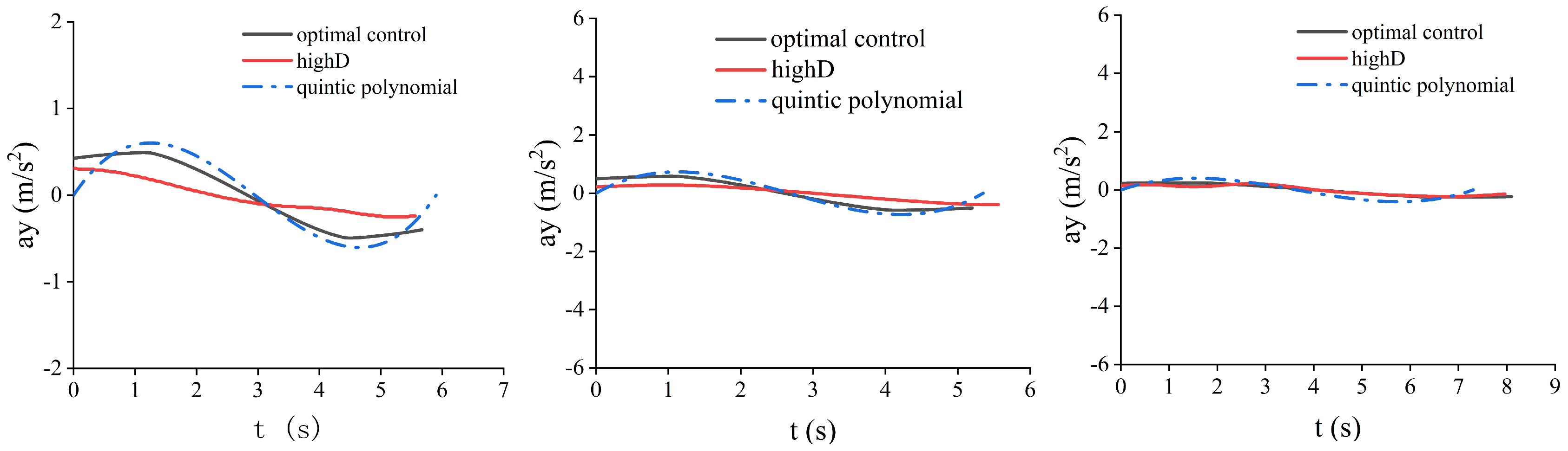
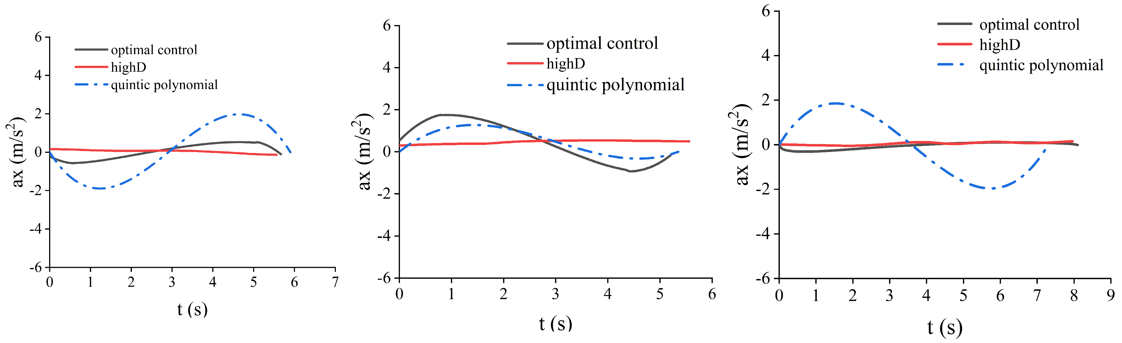
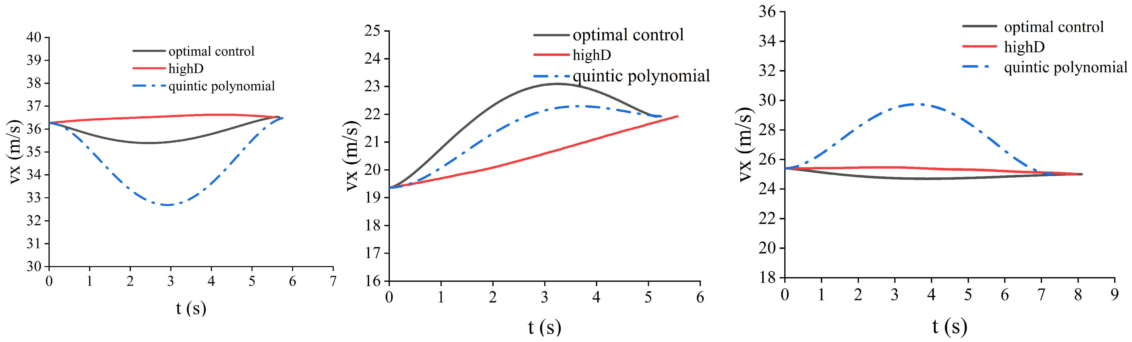
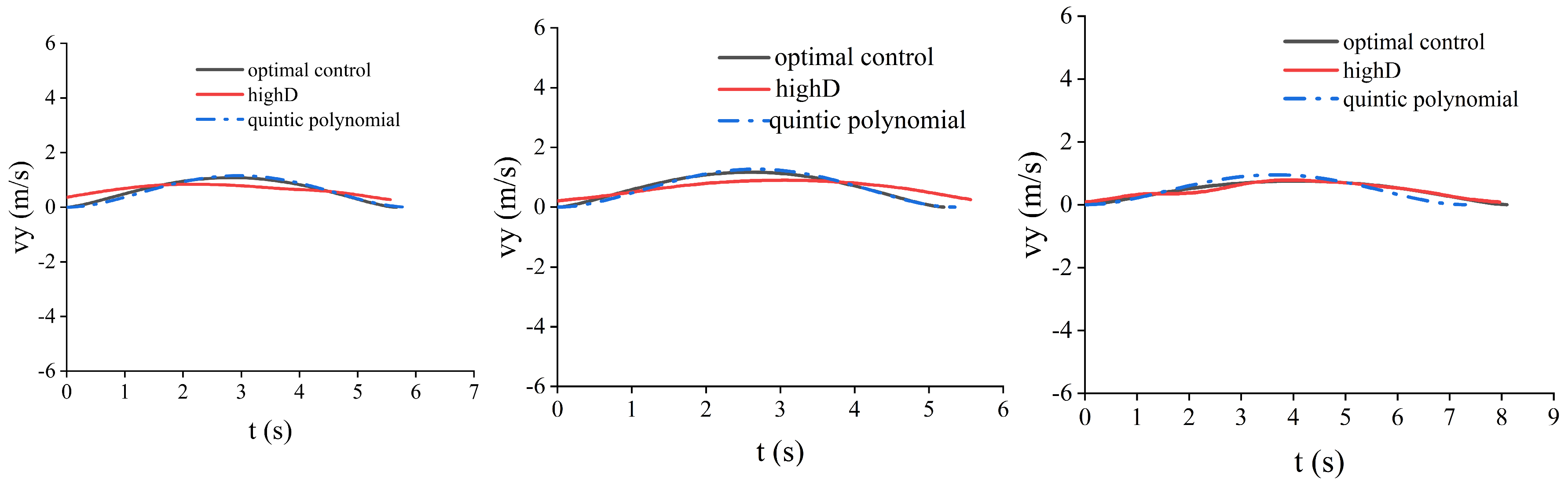
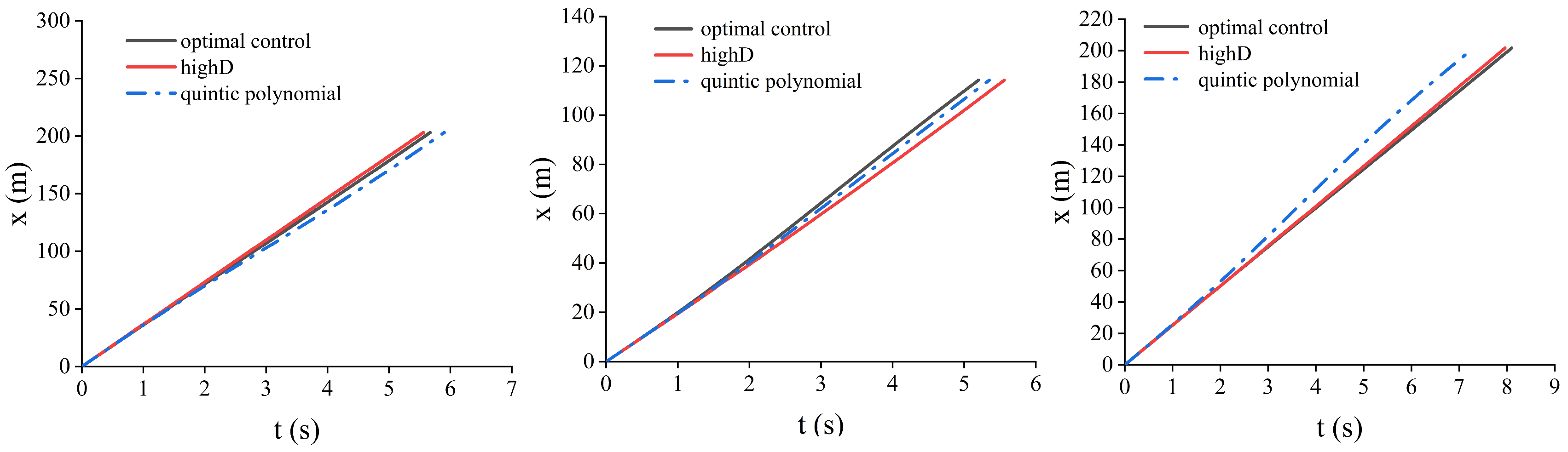
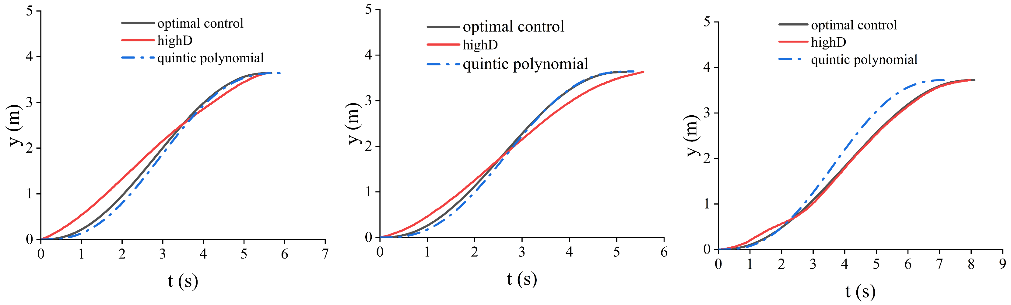
5.1. Comparative Analysis of Different Lane-Changing Algorithms and Human Driver Lane-Changing Trajectories

The vehicle is in different driving environments at the starting point and the midpoint, which leads to different requirements for the two trajectory segments. For the first segment, from the starting point to the transition (midpoint) position, even if there is some influence from computation time, the vehicle is still traveling along the lane centerline at the beginning. Considering the possible error caused by computation delay, the vehicle will only continue to move a short distance along the lane, and this minor deviation can be compensated for through prediction. Therefore, the real-time requirement for this segment is not very stringent, and the trajectory planning should primarily focus on energy efficiency. For the second segment, since the vehicle is already located at the midpoint position (between two lanes), if the computation time of the planning algorithm is too long, it may cause a mismatch between the actual and intended starting point of the second segment. This can lead to trajectory errors or even pose safety risks. As a result, the second segment must prioritize real-time performance, and energy efficiency becomes a secondary consideration. In order to determine the trajectory-planning methods used for the first- and second-segment trajectories, we compare the optimally controlled planned trajectories with the quintic polynomial trajectories. In this regard, we extracted three complete sets of driver lane-changing data under different lane-changing speeds from the highD dataset as shown in

Table 1. Traffic data.

Parameters	Longitudinal Distance (m)	Lateral Distance (m)	Longitudinal Starting Velocity (m/s)	Longitudinal Terminal Velocity (m/s)	Lateral Starting Velocity (m/s)	Lateral Terminal Velocity (m/s)
Scene 1	203.06	3.64	36.27	36.52	0.00	0.00
Scene 2	114.16	3.63	19.36	21.93	0.00	0.00
Scene 3	201.61	3.72	25.4	25.01	0.08	0.08

, representing high, medium, and low speeds during driving, respectively, and used them as templates to set up the start and end states of the lane changing; discretized the lane-changing time in steps of 0.1 s in quintic polynomial trajectory planning to generate multiple clusters of trajectories; and the trajectories that do not satisfy comfort due to excessive acceleration are eliminated from these clusters; and then a trajectory with the lowest energy consumption is selected from the remaining clusters of trajectories. In this study, we take the Nissan Leaf [42] as an example; we set the weight of the vehicle as 1521 kg, A_f = 2.3316, the slope of the road surface is set as 5°, and the CPU of the simulation device is i5-11260H, and the running memory is 16 GB.

The simulation results are shown in Figure 10 and Figure 11 (additional results are provided in Appendix A). From the trajectory comparison graph in Figure 8, we can find that the energy consumption of the trajectories generated by the optimal control is lower than the trajectories driven by the real driver in the highD dataset, as well as the trajectories planned using quintic polynomials, and the lateral and longitudinal accelerations are smaller, which makes the comfort better. From the energy consumption comparison graph in Figure 8, it is evident that the energy consumption of the trajectories planned by the optimal control is lower compared with the real driver trajectories and the quintic polynomial trajectories. The solution results for different scenarios are shown in

Table 2. Solving results for scenarios without obstacles.

		Quintic Polynomial	Optimal Control	highD
Scene 1	Energy consumption (kwh)	4.09 × 10−3	3.87 × 10−3	7.36 × 10−3
	Time(s)	5.6	5.6	5.9
Scene 2	Energy consumption (kwh)	4.98 × 10−3	4.75 × 10−3	8.37 × 10−3
	Time(s)	5.35	5.2	5.56
Scene 3	Energy consumption (kwh)	2.89 × 10−3	1.97 × 10−3	6.60 × 10−3
	Time (s)	7.25	7.91	7.96

.

Through the simulation verification under three working conditions, it can be found that the trajectory of optimal control planning has a lower lane-change duration, requires a shorter transverse displacement, consumes less energy, and is more comfortable than the trajectory of quintic polynomial planning. However, the computation time of the quintic polynomial planning is shorter, only about 7 ms, and it has very good real-time performance. Although the computation time of the optimal control planning is about 50 ms, the displacement caused by the error of the computation time is only about 1 m during the high-speed lane-changing process, and this distance error can be eliminated by computation. Therefore, the scheme of using optimal control to plan the first-segment trajectory and quintic polynomial programming to plan the second-segment trajectory is feasible in this study.

5.2. Sensitivity Analysis

According to the energy consumption cost function, the main factors affecting the energy usage during lane changing include velocity, displacement, and so on. To analyze the impact of these two factors on the energy consumption of electric vehicles, we designed two analysis scenarios. Scenario 1 investigates the effect of different longitudinal velocity differences on the energy consumption during lane changes, while Scenario 2 focuses on how different longitudinal displacements influence the energy consumption of electric vehicles during lane changing.

Scenario 1: The lateral displacement during the lane change is set to 3.75 m, and the longitudinal displacement is set to 80 m. The velocity difference between the starting and ending points is varied to study its impact on energy consumption. The initial longitudinal and lateral velocities are set to 10 m/s and 0 m/s, respectively. The final longitudinal velocities are set to 10 m/s, 11 m/s, 12 m/s, 13 m/s, 14 m/s, and 15 m/s, while the final lateral velocity remains 0 m/s. For each of these six conditions, the lane-changing time is adjusted to determine the trajectory with the best energy efficiency. As a result, six energy consumption curves are obtained, as illustrated in Figure 12a.

Scenario 2: The initial longitudinal and lateral velocities of the vehicle during the lane change are set to 18 m/s and 0 m/s, respectively. The final longitudinal and lateral velocities are set to 20 m/s and 0 m/s, respectively. The lateral displacement is fixed at 3.75 m, while the longitudinal displacement is set to 50 m, 60 m, 70 m, 80 m, 90 m, and 100 m. For each of these six conditions, the lane-changing time is adjusted to determine the most energy-efficient trajectory. As a result, six energy consumption curves are obtained, as shown in Figure 12b.

Based on the simulation results shown in Figure 12a, we observe that the energy consumption of electric vehicles increases with larger velocity differences—specifically, when the longitudinal velocity at the end of the lane change is higher. This is because a greater velocity difference requires the vehicle to accelerate more aggressively within a limited space, resulting in a higher energy demand. In addition, an increased velocity significantly raises aerodynamic drag, which is proportional to the square of the velocity. These combined effects lead to a noticeable rise in energy consumption as the velocity difference increases. This result suggests that in energy-efficient lane-change planning, it is advisable to minimize the velocity difference between the start and endpoints.

From the simulation results shown in Figure 12b, we find that energy consumption first decreases and then increases with increasing longitudinal displacement. When the displacement is small, the vehicle must complete the lane change within a shorter distance, which requires a larger acceleration and results in a higher energy consumption. As the displacement increases, the planner has more space to generate smoother trajectories, thereby reducing energy use. However, when the longitudinal displacement exceeds a certain range, the total path length and lane-change time increase significantly, which causes the energy consumption to rise again. These results indicate that a moderate longitudinal displacement can improve energy efficiency, while extreme values may lead to suboptimal performance.

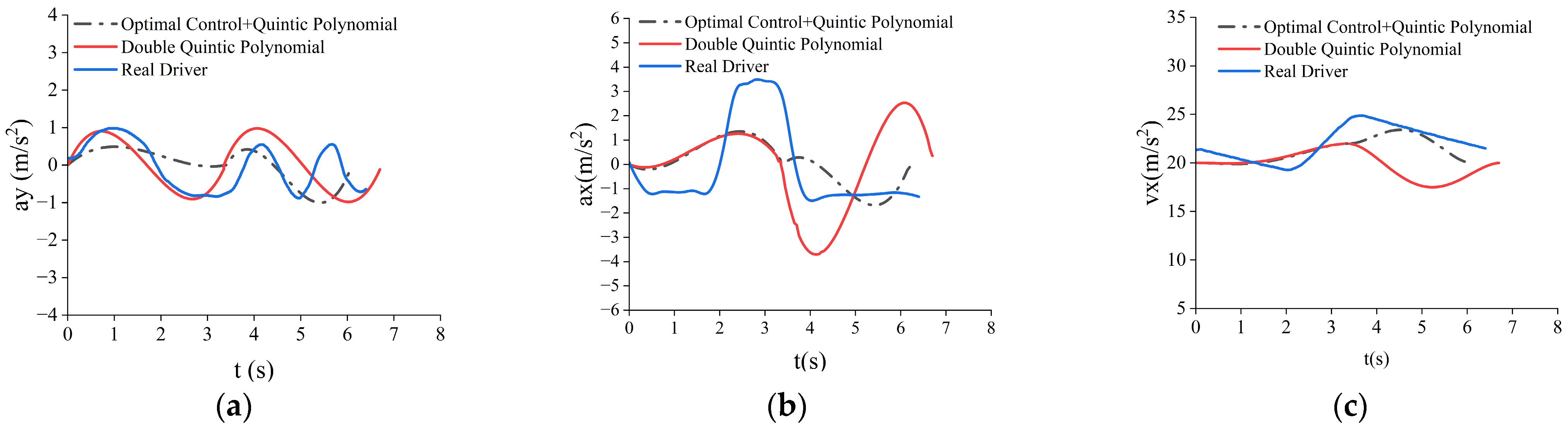
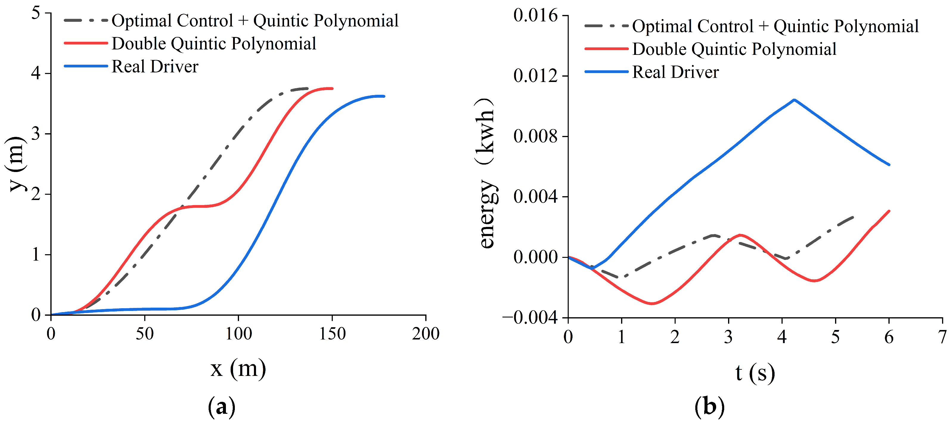
5.3. Comparative Analysis with Typical Automatic Lane-Change Models and Real Driver Lane-Change Trajectories

In order to verify the performance effect of the automatic lane-changing model proposed in this paper, this model is compared and analyzed with the automatic lane-changing model with double quintic polynomials previously proposed by Niu et al. [23] and others, as well as real driver lane-changing trajectories, and two kinds of lane-changing scenarios are set up, corresponding to a lane change by the ego vehicle at a lower speed and at a higher speed, respectively, and the scenarios are set up as shown in Figure 13. The real-driver lane-changing trajectory is acquired by the driving simulator, and the driving test scene is shown in Figure 14. The specific experimental method is as follows: a total of two drivers are set up to participate in the experiment, and the two drivers have rich driving experience, and each driver carries out the lane-changing operation 10 times for each scenario, and a total of 20 sets of experimental data are collected, from which the lane-changing trajectory with the lowest energy consumption is selected as a target for comparison.

(1) Dynamic Lane-Change Scenario 1

The distance between the ego vehicle and the obstacle vehicle ahead in its own lane can be determined by the minimum headway time distance and the ego vehicle speed [43], and the headway time distance is shown in Equation (42).

$${\mathrm{d}}_{\mathrm{i}}={\mathrm{v}}_{\mathrm{i}}\times {\mathrm{t}}_{\mathrm{i}}$$

(42)

where d_i is the limit headway, and the unit is m. v_i is the auto-vehicle speed, and the unit is m/s. t_i is for the shortest headway, and the unit is s; it generally takes 3 s.

In Scenario 1, suppose the ego vehicle A is traveling at an initial longitudinal velocity of 26 m/s; the obstacle vehicle in front is traveling at an initial longitudinal velocity of 20 m/s and decelerating at a deceleration of 2 m/s²; and the longitudinal distance between the two, d₁, is 78 m; and at this time, it is essential to perform a lane change to avoid a collision. The vehicle ahead in the target lane at this time has a longitudinal velocity of 30 m/s and 1 m/s² deceleration; first there is acceleration for 3 s; after 1.5 m/s² deceleration, there is uniform deceleration; the two initial moments of the longitudinal distance d₂ is 13 m; the target lane behind the vehicle has a 26 m/s uniform speed; the two initial moments of the longitudinal distance d₃ is 60 m; set the target speed of the lane change for 26 m/s. (From the results of the previous sensitivity analysis, it can be found that the smaller the speed difference between the starting point and the endpoint in the process of lane changing, the more the energy consumption during lane changing will decrease, so the target speed is set to be the same as the speed of the initial point). The target speed is set to be the same as the starting speed.

As shown in Figure 15 (the rest of the pictures are shown in the Appendix A), after substituting the optimal control model, it obtains that the first time needed for changing lanes is 2.7 s, and the location of the midpoint of the changing of lanes is calculated to be (70, 1.8, 26, 1.03); and the second segment of the quintic polynomial planning calculates the time of the changing of lanes to be 2.8 s and obtains the endpoint location to be (140, 3.75, 26, 0). As shown in Figure 15a, the energy consumption of the trajectory planned by the optimal control combined with the quintic polynomial is reduced by 15% compared with the double quintic polynomial and 54.83% compared with the energy consumption of the trajectory driven by the real driver. Moreover, the optimal control + quintic polynomial method lane-changing trajectory has the advantages of a smaller lateral acceleration, smoother speed change, better comfort in lane changing, and smaller transverse displacement of lane changing (from the previous sensitivity analysis, a smaller longitudinal displacement of lane changing helps to reduce the energy consumption of lane changing) compared with the other two trajectories.

(2) Dynamic lane-change Scenario 2

In Scenario 2, the initial moment from the vehicle A to 30 m/s initial speed, the obstacle in front of the vehicle B₁ to 26 m/s initial speed, and to 2 m/speed reduction has been decelerating; at this time, the lateral distance between the two vehicles d₁ is a 90 m target lane in front of vehicle B₂ at 33 m/s speed; the first 2 m/decelerated 2 s, after 1 m/accelerated 2 s and then maintain a uniform speed. At this point, the lateral gap between the two vehicles d₂ is 16 m. The target lane is behind the vehicle B₃ at this time to a 30 m/s speed driving at a constant speed; at this moment, the lateral distance between the two vehicles d₃ is 44 m. The target speed of the lane change is 30 m/s.

As shown in Figure 16 (the rest of the pictures are shown in the Appendix A), the parameters will be brought into the optimal control model; to obtain the first section of the time to change lanes is 2.9 s; the location of the midpoint of changing lanes is (86, 1.8, 30, 0.68). The time of the second segment of the lane change is 3.4 s, and the position of the endpoint of the lane change is (190, 3.75, 30, 0). As shown in Figure 16a, the energy consumption of the trajectory planned by optimal control combined with quintic polynomials in the second scenario is 10.44% lower than that of double quintic polynomials and 27.43% lower than that of the real driver’s driving trajectory, and the lane-changing trajectory of optimal control + quintic polynomials in the same Scenario 2 has a smaller lateral acceleration and longitudinal acceleration, smoother velocity change, smaller longitudinal displacement, and more comfortable lane-changing than the other two.

(3) Dynamic lane change Scenario 3

In Scenario 3, at the initial moment, the ego vehicle travels at 20 m/s, while the obstacle vehicle ahead in the current lane moves at 18 m/s. The obstacle vehicle first decelerates at 2 m/s² for 2 s and then uniformly accelerates at 1 m/s², with an initial separation of 60 m between the two vehicles. In the target lane, the lead vehicle travels at 22 m/s and initially accelerates uniformly at 1 m/s² for 3.5 s before decelerating uniformly at 2 m/s²; at the initial moment, the gap between the lead vehicle and the ego vehicle is 10 m. Furthermore, the target lane’s following vehicle starts at 18 m/s with a constant speed for 3 s and then uniformly accelerates at 2 m/s², with an initial gap of 10 m between it and the ego vehicle. The desired lane-change target speed is set at 20 m/s, matching the ego vehicle’s initial speed.

At the initial moment, the feasibility of a lane change is assessed, and the system enters the trajectory-planning module. By substituting the parameters into the optimal control model, the lane-change duration for the first segment is determined to be 3.4 s, with the midpoint of the lane change located at (70, 1.8, 22, 0.8). The second segment has a duration of 2.7 s, and the endpoint of the lane change is (130, 3.75, 20, 0). Figure 17a presents a comparison between the trajectories planned using the optimal control combined with a quintic polynomial, the double quintic polynomial lane-change model, and trajectories from human drivers. It can be observed that the trajectory obtained by the optimal control + quintic polynomial approach is significantly smoother than the other two trajectories, as illustrated in Figure 17a. In the second scenario, the trajectory planned by the optimal control coupled with the quintic polynomial reduces energy consumption by 14.76% compared to the double quintic polynomial model and by 40.48% compared to the trajectory of a human driver. Therefore, the proposed optimal control + quintic polynomial trajectory-planning model in this chapter achieves better energy efficiency, as shown in Figure 17b.

The segmented trajectory-planning method proposed in this study, which combines optimal control with quintic polynomials, demonstrates excellent performance in simulations under three typical lane-changing scenarios: low-speed, medium-speed, and high-speed. Compared with the traditional double quintic polynomial trajectory planning method [23], the proposed approach reduces energy consumption by approximately 14%. When compared with human-driven lane-changing behavior, the energy savings reach approximately 40%.This performance surpasses that of the energy-optimized quintic polynomial trajectory-planning method proposed in [31], which achieved only about a 6% reduction in energy consumption compared to the traditional quintic polynomial approach. Moreover, the trajectories generated by the proposed method exhibit smaller variations in longitudinal velocity during the lane-change process, which is consistent with the conclusion presented in [32] that smoother velocity transitions during lane changes lead to a lower energy consumption. The simulation results under the three scenarios are shown in

Table 3. Solution results for scenarios with obstacles.

Parameters		Double Quintic Polynomial	Optimal Control + Quintic Polynomial	Real Driver
Scene 1	Energy consumption (kwh)	3.22 × 10−3	2.76 × 10−3	6.12 × 10−3
	Time (s)	5.4	6	6
Scene 2	Energy consumption (kwh)	3.16 × 10−3	2.83 × 10−3	3.91 × 10−3
	Time (s)	6.7	6.28	7.26
Scene 3	Energy consumption (kwh)	3.097 × 10−3	2.646 × 10−3	4.439 × 10−3
	Time (s)	6.7	6.1	6.4

.

6. Conclusions

To develop an energy-efficient trajectory for lane changes in smart electric vehicles in dynamic traffic scenarios, this paper presents a lane-changing trajectory-planning model that combines optimal control and quintic polynomials; firstly, the whole lane-changing trajectory transit location is divided into two segments, and optimal control planning is used in the first-segment planning, and quintic polynomial planning is used in the second-segment planning. Based on simulation experiments, this study draws the following conclusions:

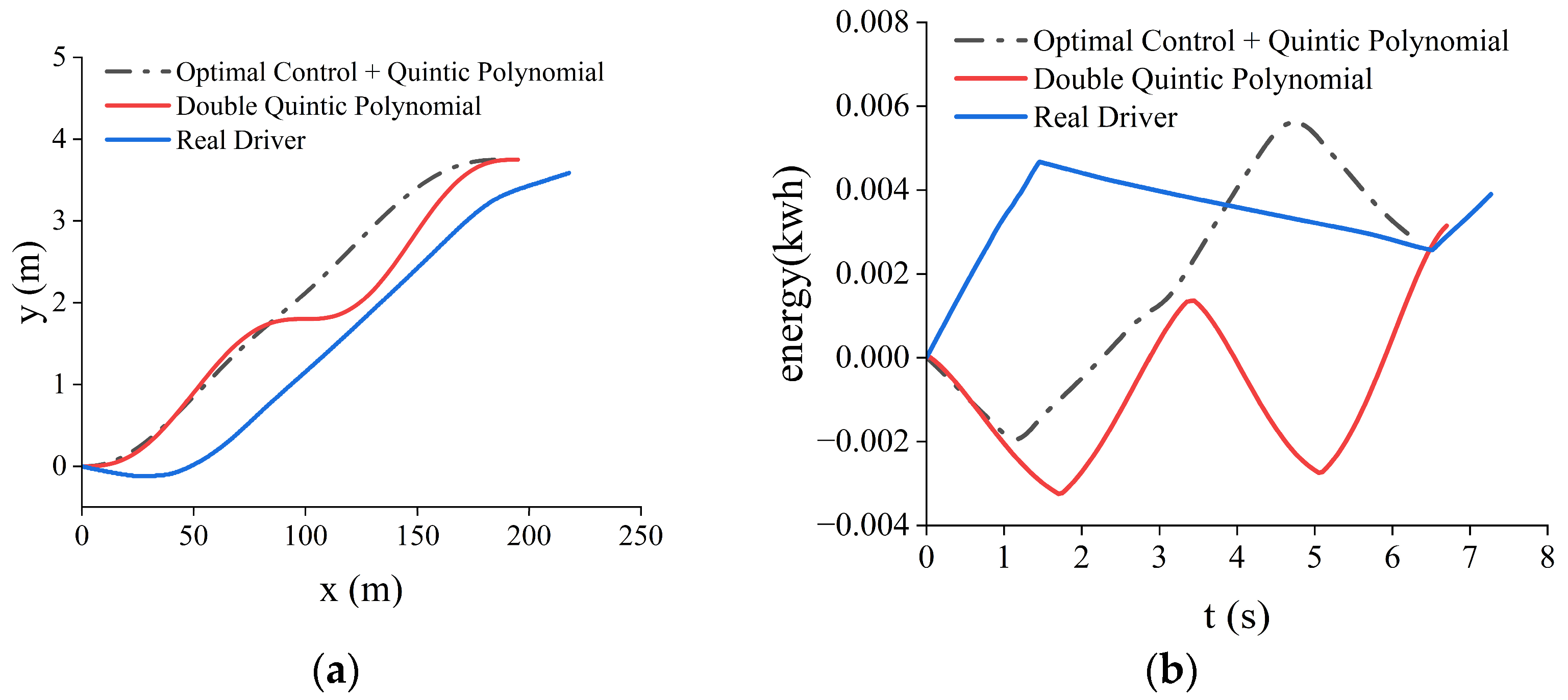
• The lane-change trajectory-planning method combining optimal control and quintic polynomials, compared with the double quintic polynomial real-time lane-change trajectory and the real-driver lane-change trajectory proposed by the previous scholars, can realize a better lane-changing economy under the premise of meeting the safety of the lane-changing process;
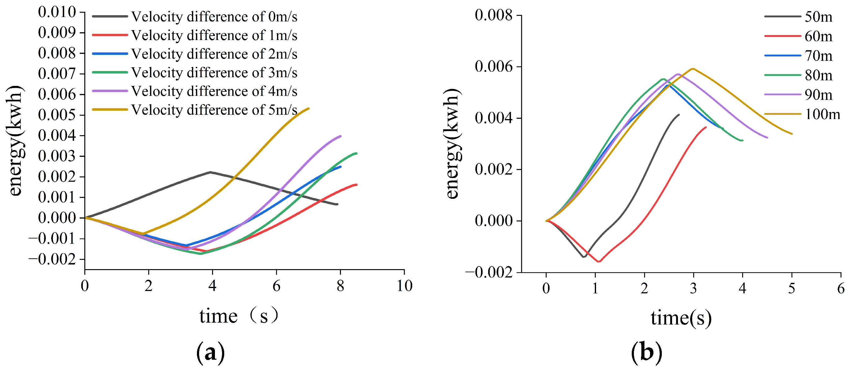
• Lane-change displacement and lane-change speed difference have a greater effect on the energy consumption of an electric vehicle. As the longitudinal displacement of the lane-change increases, the energy consumption of the lane-change firstly decreases and then increases, and the smaller the speed difference between the start point and the endpoint of the lane change, the lower the energy consumption;
• The smaller the speed difference between the start and completion of the lane change, the lower the energy consumption.

Based on the findings of this study, several future research directions can be pursued, including but not limited to the following:

• Incorporating the effects of different vehicle dimensions and sensor measurement errors into the trajectory-planning process to enhance the generalizability and adaptability of the proposed method;
• Investigating trajectory-planning strategies under more complex traffic scenarios, such as urban intersections and multi-lane congested environments;
• Extending the current offline trajectory-planning algorithm to real-world vehicle applications and validating its real-time performance and robustness through on-road testing.

References

1. He, J.; Qu, J.; Zhang, J.; He, Z. The impact of a single discretionary lane change on surrounding traffic: An analytic investigation. IEEE Trans. Intell. Transp. Syst. 2022, 24, 554–563. [Google Scholar] [CrossRef]
2. Liu, P.; Jia, H.; Zhang, L.; Wang, Z. Autonomous lane-changing trajectory planning for intelligent vehicles on structured roads. J. Mech. Eng. 2023, 59, 271–281. [Google Scholar] [CrossRef]
3. Li, J.; Zhou, W.; Tang, S. Adaptive fitting-based trajectory planning for lane-changing obstacle avoidance in intelligent vehicles. Automot. Eng. 2023, 45, 1174–1183. [Google Scholar] [CrossRef]
4. Hu, L.; Zhong, Y.; Huang, J.; Du, R.H.; Zhang, X. Optimal vehicle path planning algorithm considering signalized intersection delay. Automot. Eng. 2018, 40, 1223–1229. [Google Scholar] [CrossRef]
5. Hu, L.; Zhou, D.; Huang, J.; Du, R.; Zhang, X. Optimal path planning for electric vehicles considering signaling and energy consumption. Automot. Eng. 2021, 43, 641–649. [Google Scholar] [CrossRef]
6. Hu, J.; Zhang, Z.; Chen, R.; Ruipeng, C.; Haoyan, L.; Qi, Z.; Hui, C. A joint spatio-temporal planning method for intelligent vehicles based on improved hybrid A*. Automot. Eng. 2023, 45, 1123–1133. [Google Scholar] [CrossRef]
7. Boriboonsomsin, K.; Barth, M.J.; Zhu, W.; Vu, A. Eco-routing navigation system based on multisource historical and real-time traffic information. IEEE Trans. Intell. Transp. Syst. 2012, 13, 1694–1704. [Google Scholar] [CrossRef]
8. Buzachis, A.; Celesti, A.; Galletta, A.; Wan, J.; Fazio, M. Evaluating an application-aware distributed Dijkstra shortest path algorithm in hybrid cloud/edge environments. IEEE Trans. Sustain. Comput. 2021, 7, 289–298. [Google Scholar] [CrossRef]
9. Majumder, S.; Prasad, M.S. Three dimensional D* algorithm for incremental path planning in uncooperative environment. In Proceedings of the 2016 3rd International Conference on Signal Processing and Integrated Networks (SPIN) 2016, Noida, India, 11–12 February 2016; pp. 431–435. [Google Scholar] [CrossRef]
10. An, L.; Chen, T.; Cheng, A.; Fang, W. Simulation of intelligent vehicle path planning based on artificial potential field algorithm. Automot. Eng. 2023, 45, 1174–1183. [Google Scholar] [CrossRef]
11. Peng, X.; Xie, H.; Huang, J. Research on local path planning algorithm for driverless cars. Automotive Engineering 2020, 42, 1–10. [Google Scholar] [CrossRef]
12. Taheri, E.; Ferdowsi, M.H.; Danesh, M. Fuzzy greedy RRT path planning algorithm in a complex configuration space. Int. J. Control Autom. Syst. 2018, 16, 3026–3035. [Google Scholar] [CrossRef]
13. Du, M.; Mei, T.; Chen, J.; Zhao, P.; Liang, H.W.; Huang, R.L.; Tao, X. RRT-based motion planning algorithm for intelligent vehicles in complex environments. Robotics 2015, 37, 443–450. [Google Scholar] [CrossRef]
14. Sun, Z.; Xia, B.; Xie, P.; Li, X.; Wang, J. NAMR-RRT: Neural adaptive motion planning for mobile robots in dynamic environments. arXiv 2024. [Google Scholar] [CrossRef]
15. Akbaripour, H.; Masehian, E. Semi-lazy probabilistic roadmap: A parameter-tuned, resilient and robust path planning method for manipulator robots. Int. J. Adv. Manuf. Technol. 2017, 89, 1401–1430. [Google Scholar] [CrossRef]
16. Takahashi, A.; Hongo, T.; Ninomiya, Y.; Sugimoto, G. Local path planning and motion control for AGV in positioning. In Proceedings of the IEEE/RSJ International Workshop on Intelligent Robots and Systems (IROS’89): The Autonomous Mobile Robots and Its Applications 1989, Tsukuba, Japan, 4–6 September 1989; pp. 392–397. [Google Scholar] [CrossRef]
17. Wang, W.; Chen, H.; Ma, J. Intelligent vehicle path tracking based on Frenet coordinate system and control delay compensation. J. Mil. Eng. 2019, 40, 2336–2351. [Google Scholar] [CrossRef]
18. Ren, D.B.; Zhang, J.Y.; Zhang, J.M.; Cui, S. Trajectory planning and yaw rate tracking control for lane changing of intelligent vehicle on curved road. Sci. China Technol. Sci. 2011, 54, 630–642. [Google Scholar] [CrossRef]
19. Chu, K.; Lee, M.; Sunwoo, M. Local path planning for off-road autonomous driving with avoidance of static obstacles. IEEE Trans. Intell. Transp. Syst. 2012, 13, 1599–1616. [Google Scholar] [CrossRef]
20. Tang, B.; Xu, Z.; Jiang, H.; Cai, Y.; Hu, Z.; Yang, Z. Vehicle lane-changing obstacle avoidance trajectory planning based on segmental optimization. Automot. Eng. 2022, 44, 831–841. [Google Scholar] [CrossRef]
21. Deng, H.; Ma, B.; Zhao, H.; Lyu, L.; Liu, Y. Path planning and trajectory tracking control for emergency obstacle avoidance of autonomous vehicles. J. Mil. Eng. 2020, 41, 585. [Google Scholar] [CrossRef]
22. Luo, Y.; Wang, Y.; Cao, K.; Li, K. A dynamic automated lane change maneuver based on vehicle-to-vehicle communication. Transp. Res. Part C Emerg. Technol. 2016, 62, 87–102. [Google Scholar] [CrossRef]
23. Niu, G.; Li, W.; Wei, H. Intelligent vehicle lane-changing trajectory planning based on double-fifth degree polynomials. Automot. Eng. 2021, 43, 978–986+1004. [Google Scholar] [CrossRef]
24. Hu, L.; Yang, D.Z.; Zhang, X.; Zhang, J.; Liao, J.C. Dynamic path planning for overtaking and lane changing of intelligent vehicles based on DQP-LMPC. J. Mech. Eng. 2024, 60, 1–11. Available online: https://link.cnki.net/urlid/11.2187.TH.20240418.1524.042 (accessed on 1 February 2025).
25. Chen, L.; Qin, D.; Xu, X.; Cai, Y.; Xie, J. A path and velocity planning method for lane-changing collision avoidance of intelligent vehicles based on cubic 3-D Bezier curve. Adv. Eng. Softw. 2019, 132, 65–73. [Google Scholar] [CrossRef]
26. Wang, Q.; Li, D.; Zeng, J.; Peng, X.; Wei, L.; Du, W. A diagnostic method of freight wagons hunting performance based on wayside hunting detection system. Measurement 2024, 227, 114274. [Google Scholar] [CrossRef]
27. Bai, Y. Research on Intelligent Vehicle Trajectory Planning Considering Economy. Doctoral Dissertation, Jilin University, Changchun, China, 2021. [Google Scholar]
28. Al-Wreikat, Y.; Serrano, C.; Sodré, J.R. Driving behaviour and trip condition effects on the energy consumption of an electric vehicle under real-world driving. Appl. Energy 2021, 297, 117096. [Google Scholar] [CrossRef]
29. Hu, L.; Tian, Q.; Zou, C.; Huang, J.; Ye, Y.; Wu, X. A study on energy distribution strategy of electric vehicle hybrid energy storage system considering driving style based on real urban driving data. Renew. Sustain. Energy Rev. 2022, 162, 112416. [Google Scholar] [CrossRef]
30. Yao, Z.; Deng, H.; Wu, Y.; Zhao, B.; Li, G.; Jiang, Y. Optimal lane-changing trajectory planning for autonomous vehicles considering energy consumption. Expert Syst. Appl. 2023, 225, 120133. [Google Scholar] [CrossRef]
31. Nie, Z.; Farzaneh, H. Energy-efficient lane-change motion planning for personalized autonomous driving. Appl. Energy 2023, 338, 120926. [Google Scholar] [CrossRef]
32. Song, R.; Zhang, X.; Zhang, H.; Dai, Y.; Zhu, Y.; Tian, S. Energy-efficient lane change trajectory planning for highway traffic scenarios considering different driving needs. Appl. Sci. 2023, 13, 13184. [Google Scholar] [CrossRef]
33. Sun, C.; Liu, B.; Sun, F. A review of research on energy-saving planning and control technologies for new energy vehicles. J. Automot. Saf. Energy 2022, 13, 593–616. [Google Scholar] [CrossRef]
34. Ma, C.; Li, D. A review of vehicle lane change research. Phys. A Stat. Mech. Its Appl. 2023, 626, 129060. [Google Scholar] [CrossRef]
35. Jula, H.; Kosmatopoulos, E.B.; Ioannou, P.A. Collision avoidance analysis for lane changing and merging. IEEE Trans. Veh. Technol. 2000, 49, 2295–2308. [Google Scholar] [CrossRef]
36. Ding, H.; Li, W.; Xu, N.; Zhang, J. An enhanced eco-driving strategy based on reinforcement learning for connected electric vehicles: Cooperative velocity and lane-changing control. J. Intell. Connect. Veh. 2022, 5, 316–332. [Google Scholar] [CrossRef]
37. Mehlig, D.; Staffell, I.; Stettler, M.; ApSimon, H. Accelerating electric vehicle uptake favours greenhouse gas over air pollutant emissions. Transp. Res. Part D Transp. Environ. 2023, 124, 103954. [Google Scholar] [CrossRef]
38. Zhao, S.J.; Heywood, J.B. Projected pathways and environmental impact of China’s electrified passenger vehicles. Transp. Res. Part D Transp. Environ. 2017, 53, 334–353. [Google Scholar] [CrossRef]
39. Fiori, C.; Ahn, K.; Rakha, H.A. Power-based electric vehicle energy consumption model: Model development and validation. Appl. Energy 2016, 168, 257–268. [Google Scholar] [CrossRef]
40. Krajewski, R.; Bock, J.; Kloeker, L.; Eckstein, L. The highD dataset: A drone dataset of naturalistic vehicle trajectories on German highways for validation of highly automated driving systems. In Proceedings of the 2018 21st International Conference on Intelligent Transportation Systems (ITSC), Maui, HI, USA, 4–7 November 2018; pp. 2118–2125. [Google Scholar] [CrossRef]
41. Guo, Y.; Su, Y.; Fu, R.; Yuan, W. Influence of lane-changing maneuvers on passenger comfort of intelligent vehicles. China J. Highw. Transp. 2022, 35, 221–230. [Google Scholar] [CrossRef]
42. Nissan, L. Nissan Leaf; Nissan Corporation: Yokohama, Japan, 2010. [Google Scholar]
43. Li, S.; Zhang, M. Research on intelligent vehicle lane-changing path planning based on double-fifth degree polynomials. J. Nanjing Univ. Inf. Eng. 2024, 16, 155–163. [Google Scholar] [CrossRef]
Figure 1. Technical flowchart.
Sustainability 17 04235 g001
Figure 2. Lane-changing scenario diagram.
Sustainability 17 04235 g002
Figure 3. The edge collision point between the ego vehicle A and the preceding vehicle B1 in the current lane.
Sustainability 17 04235 g003
Figure 4. The edge collision point between the ego vehicle A and the preceding vehicle B2 in the target lane.
Sustainability 17 04235 g004
Figure 5. The edge collision point between the ego vehicle A and the following vehicle B3 in the target lane.
Sustainability 17 04235 g005
Figure 6. Lane-change diagram of the first segment.
Sustainability 17 04235 g006
Figure 7. Distribution of longitudinal acceleration, maximum transverse velocity.
Sustainability 17 04235 g007
Figure 8. Lane-change diagram of the second segment.
Sustainability 17 04235 g008
Figure 9. Cluster of quintic polynomial trajectories.
Sustainability 17 04235 g009
Figure 10. Comparison of trajectories for different scenarios. (a) Scene 1; (b) Scene 2; (c) Scene 3.
Sustainability 17 04235 g010
Figure 11. Comparison of energy consumption in different scenarios. (a) Scene 1; (b) Scene 2; (c) Scene 3.
Sustainability 17 04235 g011
Figure 12. Sensitivity analysis results. (a) Scenario 1; (b) Scenario 2.
Sustainability 17 04235 g012
Figure 13. Schematic diagram of lane change.
Sustainability 17 04235 g013
Figure 14. Driver driving data acquisition simulation system.
Sustainability 17 04235 g014
Figure 15. Simulation results of Scenario 1 with obstacles. (a) Channel-change comparison chart; (b) comparison chart of energy consumption for lane change.
Sustainability 17 04235 g015
Figure 16. Simulation results for Scenario 2 with obstacles. (a) Channel-change comparison chart; (b) comparison chart of energy consumption for lane change.
Sustainability 17 04235 g016
Figure 17. Simulation results for Scenario 3 with obstacles. (a) Channel-change comparison chart; (b) comparison chart of energy consumption for lane change.
Sustainability 17 04235 g017