Modeling the Process of Crop Yield Management in Hydroagro-Landscape Saline Soils

Abstract

To study the impact of soil salinity type and degree in irrigated lands on the process of crop yield formation, multiparametric and single-parameter mathematical models were used. The methodological basis of the study was the materialist theory of scientific knowledge (analysis and synthesis) and the laws of ecology, using graph-analytical methods based on artificial intelligence and the applied software product Microsoft Office. To create the database, an empirical method of generalizing research results was used to study the effect of soil salinity type and degree in irrigated lands on the yield of agricultural crops in various natural and climatic zones of Central Asia for the period from 1932 to 2020. Based on plotting graphs of the dependence of the relative yield of agricultural crops on the dimensionless (relative) value of soil salinity type and degree, based on research data, the following results were obtained: first, differential equations describing the studied process were derived; second, within the framework of a very high determination index confirming a strong correlation between the function arguments and yield, a system of exponential, logarithmic, and polynomial equations was obtained using the applied software product Microsoft Office, which enables the management of agricultural crop yields on saline soils; and third, it creates prerequisites for the design of ecologically sustainable agro-landscapes.

1. Introduction

The total land area of the planet is approximately 13.50 billion hectares, of which 4.8 billion hectares are agricultural lands. These lands form the basis of terrestrial ecosystems and support the production of food and agricultural raw materials for human use. Within the structure of agricultural lands, about 0.831 billion hectares consist of saline soils, comprising 0.397 billion hectares of saline soils and 0.434 billion hectares of solonetz soils, respectively [1].

Soil salinization is one of the major global issues causing the degradation of the agricultural resource potential of agricultural landscapes, particularly in desert and semi-desert zones with arid and semi-arid climates. This problem is most pronounced in regions such as the Middle East, the North China Plain, Central Asia, the South Caucasus, southern Russia, and North Africa. Salinization is a complex process in which the excessive accumulation of salts in the soil exerts a toxic effect on plant life. This can occur due to natural processes (primary salinization) or as a result of human activities (secondary salinization) [2].

The area of irrigated land worldwide accounts for only 15% of the total agricultural land area, yet it contributes to one-third of global food production [3]. According to average estimates, approximately 100 million hectares of irrigated land have become saline due to poor irrigation practices [4]. Thus, around 11% of the world’s irrigated land is already affected by salinization to some extent [5].

Due to half a century of intensive and mismanaged human activity, one of the most severe cases of soil salinization and waterlogging of agricultural lands is observed in the Aral Sea basin in Central Asia (Uzbekistan, Kazakhstan, the Kyrgyz Republic, Tajikistan, and Turkmenistan) [6,7,8]. In this region, up to 50% of irrigated land suffers from secondary salinization, and thousands of square kilometers of irrigated land have undergone degradation during the conversion of virgin lands into irrigated agricultural areas [9]. This has become a global model of uncontrolled and unregulated natural-technogenic land use and land management in irrigated agriculture [10], which is a consequence of the law of successional slowdown [11].

Thus, the functional activity of hydro-agrolandscapes was initially oriented toward rigid environmental management. According to the law of successional slowdown, in the early stages of their functioning, there is a significant increase in the productivity of agricultural lands. However, this growth eventually stabilizes at a certain level, followed by a gradual decline in biological productivity, which is accompanied by undesirable consequences, particularly secondary salinization. The primary cause of this phenomenon lies in the contradiction between the global scale of these issues and the localized approaches to their resolution. Traditionally, efforts have been directed at addressing the consequences rather than the root causes, which has disrupted almost all natural processes. Any transformation of nature is not arbitrary; it is governed by ecological laws that underpin the principles of environmental management.

The relevance of the issue under consideration is determined by the threat of the irreversible process of secondary soil salinization in the irrigated lands of Central Asia. As a result, the need arises to develop mathematical models for managing crop yields of agricultural crops. These models should be based on empirical generalizations of experimental data obtained from various soils with different types and degrees of salinity. Their universality, accuracy, and reliability are ensured by modeling multiparametric and single-parameter relationships between yield and yield-forming factors in relative values, using digital technologies.

2. Materials and Methods

2.1. Research Materials

The research database was formed based on field studies conducted by V. A. Kovda, L. I. Mamaev [12], S. S. Puruzian [13], I. S. Rabochev, V. S. Burdygin [14], M. N. Tsvylev [15], R. M. Gorbachev [16], S. M. Schmidt [17], V. A. Dukhovny, D. Umardzhanov [18], I. P. Aidarov, L. F. Pestov, T. P. Korolkov [19], and A. U. Usmanov [20]. These studies serve as the foundation for modeling the process of managing crop yields under saline soil conditions.

2.2. Principles of Constructing Mathematical Models of Agricultural Crop Yield

The driving force behind the development of modern environmental management systems is the contradiction between the unlimitedly growing needs of a developing humanity and the limited material and energy resources of nature. Based on the law of internal dynamic equilibrium, this necessitates the creation of a specific type of hydro-agrolandscapes with predefined properties, ensuring a balanced use of the resource potential of agricultural landscapes. These landscapes are designed to regulate key environmental factors affecting cultivated crops, including water, heat, light, nutrients, air, and salt regimes. Their functional representation is as follows [21]:

$${CY}_i=f\left({WS}_i,{BT}_i,{FAC}_i, {FP}_i, {GS}_i,{SS}_i\right),$$

(1)

where ${CY}_i={CCY}_i/{PCY}_i$—relative yield of agricultural crops; ${CCY}_i$—current crop yield; ${PCY}_i$—potential crop yield under optimal environmental conditions; ${WS}_i={WCAC}_{ci}/{WCAC}_{oi}$ = $d{WCAC}_{ci}/{dWCAC}_{oi}$—water supply of the crop;${WCAC}_{ci}$—current crop water consumption; ${WCAC}_{oi}$—optimal crop water consumption; $d{WCAC}_{ci}$—current crop water deficit;${dWCAC}_{oi}$—optimal crop water deficit; ${BT}_i={SCT}_i/{SBT}_i$—heat supply of the crop; ${SCT}_i$—the sum of active climatic temperatures during the period above 10 °C; ${SBT}_i$—the sum of active biological temperatures required for crop maturation; ${FAC}_i={PAR}_{mi}/{PAR}_{oi}$—light supply of the crop;${PAR}_{mi}$—the current sum of photosynthetically active radiation required for crop maturation; ${PAR}_{oi}$—the optimal sum of photosynthetically active radiation required for maximum yield;${ FP}_i={NPK}_{ci}/{NPK}_{oi}$—nutrient supply of the crop;${ NPK}_{ci}$—current content of nutrients required for yield iii; ${NPK}_{oi}$—optimal content of nutrients required for maximum yield; ${GS}_i={GISAL}_{ci}/{GISAL}_{oi}$—air supply of the crop; ${GISAL}_{ci}$—total air capacity of agricultural soil;${ GISAL}_{oi}$—optimal air capacity of agricultural soil; ${SS}_i={SCS}_{oi}/{CTSS}_{mpi}$—salt supply of the crop; ${SCS}_{oi}$—initial content of water-soluble salts in the soil’s one-meter layer; and ${CTSS}_{mpi}$—maximum permissible concentration of toxic salts in the one-meter soil layer, above which crops experience severe stress (${CCY}_i=0$).

For the vital activity of agricultural crops, heat, light, and air—being cosmic factors and natural energy sources of autotrophic nutrition—are indispensable and limit the physiological activity of crops. These factors cannot be regulated by humans in the course of agricultural production, necessitating adaptation to these natural processes. In this regard, targeted management of environmental conditions in accordance with the requirements of agricultural crops is achieved by regulating the water, nutrient, and salt regimes of the soil in agricultural landscapes. These factors belong to the terrestrial conditions of crop existence and allow for the construction of highly productive and sustainable hydro-agrolandscapes through integrated land reclamation measures.

The analysis and evaluation of the effects of life-sustaining factors for agricultural crops (water, nutrients, light, heat, air, and salts), which follow certain patterns—or ecological laws of plants—highlight the most important principles, including the law of equivalence or irreplaceability of factors [22], the law of the limiting factor or Liebig’s law of the minimum (the «Drobenek barrel») [23], the law of the optimum [24], the law of the combined action of factors (Mitscherlich–Tinmann–Baule law) [25,26], and the law of tolerance (V. Shelford’s law) [27]. These laws demonstrate the dependence of agricultural crop yield on life-supporting factors, which are characterized by two types of curves [11] (Figure 1).

The model equation, which characterizes the conditions that the yield change trajectories of agricultural crops must satisfy, based on the factors of their vital activity determined by thermal, light, air, water, and nutrient regimes of soil in agricultural landscapes, can be described using a logistic S-shaped (sigmoidal) curve (Figure 1, curve 1). This requires considering these factors at the final stage of modeling biomass production in the studied process.

An analysis of the functional dependence of agricultural crop yield on the salt regime of soil in agricultural landscapes, which is one of the main factors of their vital activity, shows (Figure 1, curve 2) that the relationship follows a hyperbolic shape, where the left branch approaches one and the right branch approaches zero. These curves correspond to the trajectories of physiological process changes.

Based on the law of the limiting (limiting) factor, or Liebig’s Law of the Minimum [11]—one of the fundamental laws in ecology, which states that among the factors influencing the life of agricultural crops, the most significant is the factor with the minimum value—it is possible to construct a logical dependence of agricultural crop yield on factors of their vital activity using the following mathematical equations:

$${CY}_i={CCY}_i/{PCY}_i={CLF}_{mini};$$

(2)

$${CCY}_i={PCY}_i·{CLF}_{mini}:$$

(3)

$$0 {\le CLF}_{mini}\le 1.0;$$

(4)

$${CLF}_{mini}=min\left|{WS}_i,{BT}_i,{FAC}_i, {FP}_i, \right|,$$

(5)

where ${CLF}_{mini}$ is the life factor of agricultural crops with the minimum value.

A distinctive feature of such logical models, characterizing the dependence of agricultural crop yield on the factors of plant life, is that the function of agricultural crop vitality from external environmental factors (thermal, light, water, air, food, and salt regimes) included in their structure must satisfy the traditional conditions of monotonicity, convexity, and homogeneity for production functions if the permissible boundaries of the change in its parameters are set by the conditions $0\le {CLF}_{mini}\le 1.0$.

2.3. Construction of Mathematical Models of Crop Yields

There is a large body of work, among which the works of E.A. Metcherlekh [22], Y.K. Ross [28], H.G. Toming [29], H.A. Moldau [30], A. Laisk, H.A. Moldau [31], O.D. Sirotenko [32], Y.A. Khvalinsky, O.D. Sirotenko [33], A.N. Polevoy, L.V. Flora [34], and Zh.S. Mustafayev et al. [35] stand out. These works make attempts to describe plant requirements for external environmental conditions using physical–statistical models of agricultural crop yield formation.

In the work by Dilli Paudel et al. [36], using information technologies, functions (or predictors) were developed for crop yield modeling, utilizing weather data and soil remote sensing from the MCYFS database at the regional level for five agricultural crops in three countries: The Netherlands, Germany, and France.

For forecasting crop yields, Michiel G.J. et al. [37], Kakabouki, I. et al. [38], U. Khan et al. [39], and Fischetti E. et al. [40] employed a meta-modeling approach, which combines a theoretically grounded crop growth model based on processes with a modeling method based on information technology. This approach prevents the model from using false functions, which is particularly important in models with high complexity.

A comprehensive approach to crop yield forecasting using calibration methods based on artificial intelligence and crop growth models was proposed by Renato Luiz et al. [41] on an integrated platform. Thus, crop yield forecasting for ensuring food security for the growing world population has become an increasingly important issue, and the use of information technologies as a potential tool that allows for the automatic extraction of features from datasets characterizing crop yield growth models is gaining significance.

One of the fundamental directions in the field of integrated regulation of plant life factors was proposed by V.V. Shabanov [42], who attempted to create a system of mathematical models in the form of differential equations describing the change in crop productivity depending on environmental conditions. The model takes the following form when ${\phi }_{min}=0 and {\phi }_{max}$ = 1:

$$S_i={\left({\phi }_i/{\phi }_{opt}\right)}^{\gamma ·{\phi }_{opt}}·{\left[\left({\phi }_{max}-{\phi }_i\right)/\left({\phi }_{max}-{\phi }_{opt}\right)\right]}^{\gamma ·\left({\phi }_{max}-{\phi }_{opt}\right)},$$

(6)

where $S_i$ is the relative productivity, defined as the ratio of current productivity to maximum productivity under the given constraints; ${\phi }_{opt}$, ${\phi }_{min}, {\mathrm{a}\mathrm{n}\mathrm{d} \phi }_{max}$ are the optimal, minimum, and maximum values of the factor under which the crop produces; γ is a dimensionless parameter that characterizes the degree of self-regulation of plants over time.

Mathematical modeling of crop yield in saline soil conditions of agricultural landscapes is a useful tool for determining the type of equations that describe this process. As the relative salt content in the soil and irrigation water increases, the relative yield decreases. This characteristic distinguishes salinity from other factors affecting the life of agricultural crops.

In the works of E. Misle [43,44], for forecasting crop yield on saline soils, the theory of allometry in biological sciences was used, where the relationship between the accumulation of any mineral nutrient and the total biomass of crops is expressed in the form of a power equation (allometric equation), reflecting remarkable scale symmetry [45]. This relationship is represented by the equation:

$$1-\left(B_s/B_i\right)={\left(S_i/S_s\right)}^{b_s},$$

(7)

where $B_s$ is the potential biomass of crops at $S_i=0$; $B_i$ is the biomass of crops under soil salinization; $S_i$ is the mineral substance or salt content in the soil; $S_s$ is the maximum allowable mineral substance or salt content in the soil, ensuring the potential biomass of agricultural crops; and $b_s$ is the algometric parameter [46,47]. The allometric parameter ($b_s$) for saline soils in agricultural landscapes, given the known values of $B_s/B_i$ and $S_i/S_s$, is determined by the following formula:

$$b_s=ln\left[1-\left(B_s/B_i\right)\right]/ln\left(S_i/S_s\right).$$

(8)

The resulting function, showing the decrease in allometric parameters ($b_s$) with increasing relative soil salinity $\left(S_i/S_s\right)$, required the use of a power function with negative allometric parameters ($b_{sd}$—the rate of decrease) to satisfy the trajectory of the studied process, which takes the form [48]:

$$B_s/B_i=1-\alpha ·{\left[\left(S_i/S_s\right)+c\right]}^{b_s·{\left[\left(S_i/S_s\right)+c\right]}^{b_{sd}}},$$

(9)

where $\alpha$ is a constant related to the steepness of the curve’s decline as the relative salt content in the soil of agricultural landscapes increases and c is a constant determining the initial point of inflection.

One of the main ecological factors limiting crop yield on saline soils is, first, the salt tolerance of agricultural crops, and second, the type and degree of soil salinization, which shape their ecological functions and services in agricultural landscapes.

Based on the development and deepening of the well-known theory of algometry in biology, new directions were formed to assess the impact of salt stress on plants caused by the accumulation of salts in the soil [3,49,50,51,52,53,54,55,56,57,58,59], which allowed [60,61,62,63] to study the impact of nitrate-soluble salts (chloride sulfate of sodium, magnesium, and calcium) on the growth and development of agricultural crops in spatial aspects across various natural-climatic zones of the world.

2.4. Methodology and Materials for Mathematical Modeling of Crop Yields

The analysis and evaluation of the impact of regulated and controlled regime-forming factors (water, salt, and nutrient regimes) on crop yield in various natural-climatic zones of the world, in both spatial and temporal aspects, have shown that they transform and integrate within the functioning of agricultural landscapes as a system of all-natural and natural-anthropogenic processes, which manifest according to the laws of nature.

The results of these studies provide valuable information about the use of saline soils in agricultural landscapes, suggesting that the study of the impact of the salt regime (${GS}_i$) within the factors of plant life, consisting of toxic salts in the soil (primarily anions such as $Cl$, ${SO}_4$, and ${HCO}_3$) dissolved in the soil solution, as well as cations of the soil exchange complex (mainly Na, Ca, and Mg content), and the $pH$ of the soil solution may be of vital importance in the context of global climate change and the exponential growth of anthropogenic salinization of agricultural land.

To design highly productive and ecologically sustainable hydro-agricultural landscapes for agricultural use on saline lands, mathematical models of the life factors of crops, consisting of toxic salts in the soil, are required for managing regime-forming factors, specifically the soil salt regime. This regime serves as a valuable tool for targeted regulation of the soil formation process and performs important landscape-forming and ecological functions.

The aim of the study is to develop mathematical models in the form of differential equations that describe changes in crop yield depending on the types of toxic salts in the soil of saline lands, using a set of experimental data obtained from studies of these processes.

The main informational resources used to create the research base include data that characterize the impact of soil salt content on crop yield in the saline landscapes of agricultural use in Central Asia and Kazakhstan, covering the period from 1939 to 2020 [64].

The studies used special methods of scientific knowledge: the allometric approach, mathematical modeling of natural processes based on the laws of ecology and principles of environmental management, and the correlation method of statistical analysis and data processing using Microsoft Office software.

3. Results

3.1. Dynamic Models of Crop Yields

The most effective tool for systemic analysis of the requirements of agricultural crops for environmental factors ensuring their viability, especially on natural and anthropogenic saline lands, is special mathematical models that reflect the dependence of crop yield on soil salt content in agricultural landscapes. A distinctive feature of the models reflecting changes in crop yield depending on soil salt content is their trajectories, which do not coincide with the trends and directions of other environmental factors (such as thermal, light, water, nutritional, and air regimes).

To ensure the accuracy of the developed mathematical models that characterize the yield change trajectories of agricultural crops from the content of toxic salts in the soil, all available information resources from the research database, created based on the study results in the conditions of Central Asia and Kazakhstan [64], are consolidated into a unified system in the form of the function ${CY}_i={CCY}_i/{PCY}_i=f\left({SS}_i\right)=f({SCS}_{oi}/{CTSS}_{mpi})$. Using this, graphs were created to illustrate the relationship between crop yield and initial soil salinity by chlorine (Figure 2) and the total toxic salts in the soil solution (Figure 3).

As seen in Figure 2 and Figure 3, the specific type of crop yield functions, describing the dynamics of toxic salt content, is determined using Microsoft Office software. The researcher’s task is to select a mathematical equation with a high correlation coefficient that satisfies the trajectory of the studied process and to include additional relations in the system that account for the influence of external factors and management interventions.

To describe the requirements of agricultural crops for soil salinity in agricultural landscapes, we use their degree of optimality, expressed by relative crop yield (${CY}_i={CCY}_i/{PCY}_i$), assuming that its decrease is directly proportional to the deviation of salt content (${SCS}_{oi}$) from its toxicity (${CTSS}_{mpi}$), i.e., ${(CTSS}_{mpi}-{SCS}_{oi}).$ Indeed, the greater the degree of optimality ${CY}_i$, the higher the $d{CY}_i/{SS}_{oi}$, meaning that any deviation from optimality leads to a deviation from ${PCY}_i$. At the same time, the larger the deviation from optimal conditions ${CY}_i$, i.e., the greater the value of (${SCS}_{oi}/{CTSS}_{mpi})$, the more sensitive the crop is to soil salt content, On the other hand, under conditions where ${SCS}_{oi}/{CTSS}_{mpi}=1$, $d{CY}_i/{dSS}_{oi}=0$, meaning there are points ${PCY}_i$, where ${SCS}_{oi}=0$, the relationship between crop yield (${CCY}_i$) and soil salt content (${SCS}_{oi}$), is described by a first-order differential equation as follows:

$$d{CY}_i/{dSS}_i=-k·{SS}_{oi}.$$

(10)

where $k$ is the proportionality coefficient that matches the dimensions of the left and right sides and characterizes the salt tolerance of crops under non-optimal conditions.

The negative sign in front of the right-hand side of the first-order differential equation, according to the allometric hypothesis, indicates a decrease in crop yield with an increase in salt content in the soil (${SCS}_{oi}/{CTSS}_{mpi}\to 1.0$).

Therefore, integrating the equation $d{CY}_i/{dSS}_i=-k·{SS}_{oi}$, with boundary conditions ${SS}_{oi}=0{CY}_i=1$ and ${SS}_{oi}=1$, ${CY}_i=0$, we obtain:

$${lnCY}_i=-k·{SS}_{oi}+A$$

(11)

or

$${lnCY}_i=-k·{SS}_{oi}+A.$$

(12)

where $A$ is the integration constant.

The constant $A$ is determined from the condition ${CY}_i=1$ when ${ SS}_{oi}=0$, so $A=0$.

Thus, we obtain:

$${lnCY}_i=-k·{SS}_{oi},$$

(13)

and by exponentiating, we obtain

$${CY}_i=\mathrm{e}\mathrm{x}\mathrm{p}(-k·{SS}_{oi}).$$

(14)

In this case, the proportionality coefficient kkk, which characterizes the salt tolerance of crops under non-optimal conditions, is calculated based on empirical data on the toxicity response of salts in saline soils as $k=lnCY/ln{SS}_{oi}$, which results in a power curve (Figure 2 and Figure 3).

As seen from Figure 2 and Figure 3, the quantitative values of the allometric coefficient ($k$), which characterize the salt tolerance of agricultural crops, are a function of the toxicity of salts in the soil. As the relative salinity ${SS}_{oi}\to 1.0$, the yield ${ CY}_i\to 0$, and this relationship can be represented as a power function with a negative allometric coefficient ($-k$). This can be expressed as $k={({SCS}_{oi}/{CTSS}_{mpi})}^b$, where $b$ is a constant that characterizes the tolerance of agricultural crops to the content of toxic salts in the soil. This is associated with the exponential decay and sharp decline of this process, which requires a detailed parametric analysis.

3.2. Linear Correlation Model of Crop Yields on Saline Lands

The linear correlation model of crop yields, dependent on factors of their life activities, was developed based on a combination of experimental and theoretical methods.

To illustrate the presented conclusions, the information resources of R. M. Gorbachev [16] were used, based on the generalization and systematization of data from scientific studies on the influence of soil salinity on the yield of agricultural crops in Central Asia and Kazakhstan. These data allowed for the creation of graphs and the derivation of exponential and logarithmic equations using Microsoft Office software (Figure 4 and Figure 5 and

Table 1. Exponential and logarithmic models of agricultural crop yield (${CY}_i={CCY}_i/{PCY}_i$) depending on the degree of soil salinity (${SS}_i{=SCS}_{oi}/{CTSS}_{mpi}$) of landscapes used for agriculture.

Agricultural Crop	Equation	$\mathbf{Determination} \mathbf{Index} \mathbf{\left(}{\mathit{R}}^2\mathbf{\right)}$
Cotton	${CY}_i=1.0742·\mathrm{e}\mathrm{x}\mathrm{p}(-2.0060·{SS}_i)$	0.9671
	${CY}_i=-0.4010·\mathrm{l}\mathrm{n}\left({SS}_i\right)+0.1393$	0.8559
Winter wheat	${CY}_i=1.1103·\mathrm{e}\mathrm{x}\mathrm{p}(-2.1200·{SS}_i)$	0.9818
	${CY}_i=-0.4070·\mathrm{l}\mathrm{n}\left({SS}_i\right)+0.0699$	0.9377
Grain corn	${CY}_i=1.1762·\mathrm{e}\mathrm{x}\mathrm{p}(-1.5490·{SS}_i)$	0.8877
	${CY}_i=-0.4420·\mathrm{l}\mathrm{n}\left({SS}_i\right)+0.0491$	0.8375
Silage corn	${CY}_i=1.4060·\mathrm{e}\mathrm{x}\mathrm{p}(-2.1750·{SS}_i)$	0.8627
	${CY}_i=-0.2470·\mathrm{l}\mathrm{n}\left({SS}_i\right)+0.4828$	0.8184
Alfalfa	${CY}_i=14440·\mathrm{e}\mathrm{x}\mathrm{p}(-2.212·{SS}_i)$	0.8462
	${CY}_i=-0.2444·\mathrm{l}\mathrm{n}\left({SS}_i\right)+0.4834$	0.8328
Sugar beet	${CY}_i=1.5282·\mathrm{e}\mathrm{x}\mathrm{p}(-2.070·{SS}_i)$	0.7206
	${CY}_i=-0.1311·\mathrm{l}\mathrm{n}\left({SS}_i\right)+0.7160$	0.8328
Sunflower	${CY}_i=1.3965·\mathrm{e}\mathrm{x}\mathrm{p}(-2.2630·{SS}_i)$	0.8831
	${CY}_i=-0.2180·\mathrm{l}\mathrm{n}\left({SS}_i\right)+0.5482$	0.7623
Potato	${CY}_i=1.3364·\mathrm{e}\mathrm{x}\mathrm{p}(-1.5960·{SS}_i)$	0.7674
	${CY}_i=-0.4220·\mathrm{l}\mathrm{n}\left({SS}_i\right)+0.1031$	0.7712
Tomato	${CY}_i=1.4568·\mathrm{e}\mathrm{x}\mathrm{p}(-2.1440·{SS}_i)$	0.8398
	${CY}_i=-0.2531·\mathrm{l}\mathrm{n}\left({SS}_i\right)+0.5169$	0.8119
Pea	${CY}_i=1.2164·\mathrm{e}\mathrm{x}\mathrm{p}(-1.989·{SS}_i)$	0.9573
	${CY}_i=-0.4270·\mathrm{l}\mathrm{n}\left({SS}_i\right)+0.0315$	0.9719
Sweet pepper	${CY}_i=1.4081·\mathrm{e}\mathrm{x}\mathrm{p}(-2.1540·{SS}_i)$	0.8737
	${CY}_i=-0.3540·\mathrm{l}\mathrm{n}\left({SS}_i\right)+0.1592$	0.9125
Eggplant	${CY}_i=1.4081·\mathrm{e}\mathrm{x}\mathrm{p}(-2.1154·{SS}_i)$	0.8737
	${CY}_i=-0.2620·\mathrm{l}\mathrm{n}\left({SS}_i\right)+0.4360$	0.8389

).

The analysis of the exponential and logarithmic functions of agricultural crop yield (${CY}_i$) as a function of soil salinity (${SS}_i$) in agricultural landscapes shows that the regression coefficient (model parameter) ($\alpha$), which characterizes the change in the yield of agricultural crops (${∆CY}_i$) with changes in soil salinity (${∆SS}_i$), can be derived from the equation with a negative sign: ${∆CY}_i=\left({CY}_i-b\right)=-\alpha ·\mathrm{l}\mathrm{n}\left({SS}_i\right)$ and for ${SS}_i=0$, ${∆CY}_i=-\alpha$. As seen in Figure 4 and Table 1, the quantitative value of the regression coefficient (model parameter) (α), as a proportionality coefficient (k), depends on the salt tolerance of agricultural crops, and the relationship between them is described by a linear equation $k=\beta ·\alpha +c\to k=\mathrm{3,2}·\alpha +0.32$. This equation characterizes the qualitative aspect of the reproduction process.

The free term of the logarithmic function ${CY}_i=-\alpha ·\mathrm{l}\mathrm{n}\left({SS}_i\right)+b$, which represents the dependency of agricultural crop yield (${CY}_i$) on soil salinity (${SS}_i$) in agricultural landscapes, is considered a constant value ($b$), as an absolute parameter.

To assess the quality of the exponential and logarithmic functions of crop yields based on soil salinity in agricultural landscapes, the square of the logarithmic correlation coefficient (R²), known as the coefficient of determination, is calculated. This coefficient is a measure of the level of approximation, which showed that their quantitative value is very high, varying depending on the type of crop from 0.7774 to 0.9897. This indicates good convergence and ensures highly reliable practical calculations based on these models.

The maximum permissible content of toxic salts in the top meter of soil (${CTSS}_{mpi}$), at which the yield of agricultural crops becomes zero (${CCY}_i=0$), depends on their salt tolerance. For different crops, the threshold values are as follows: Cotton: 1.40%; Winter wheat: 1.20%; Grain corn: 0.90%; Silage corn: 1.60%; Alfalfa: 1.60%; Sunflower: 1.70%; Potato: 0.90%; Tomato: 1.50%; Peas: 0.80%; Sweet pepper: 1.20%; Eggplant: 1.50%; Beetroot: 1.80% (expressed as percentages of dry matter weight).

Summarizing the results of studying the yield formation processes of various agricultural crops under saline soil conditions in agricultural landscapes of Central Asia and Kazakhstan, it can be concluded that along all exponential trajectories, according to the law of diminishing fertility (which directly depends on soil salinity), the maximum decrease in the yield of agricultural crops from ${CY}_i=1.0 to {CY}_i=0.4$ occurs from ${SS}_i=0$ to ${SS}_i=0.5$ and, subsequently, from ${SS}_i=0.6$ to ${SS}_i=1.0$, the decrease stabilizes at levels between ${CY}_i=0.3$ to ${CY}_i=0$.

In saline soils, trace elements—chemical elements essential for vital processes in agricultural crops—are found in very small amounts (less than 0.001%). To establish a relationship between crop yield and the mobile forms of aluminum in soils of various compositions, research results from Central Asia and Kazakhstan were used [19]. Statistical analysis of the collected data and the creation of corresponding graphs were carried out using the correlation method with Microsoft Office software (Figure 6 and

Table 2. Polynomial model of crop yield (${CY}_i={CCY}_i/{PCY}_i$) depending on the content of mobile forms of aluminum in the soil (${SS}_i{=SCS}_{oi}/{CTSS}_{mpi}={Al}_i/{Al}_{ti}$) in agricultural landscapes.

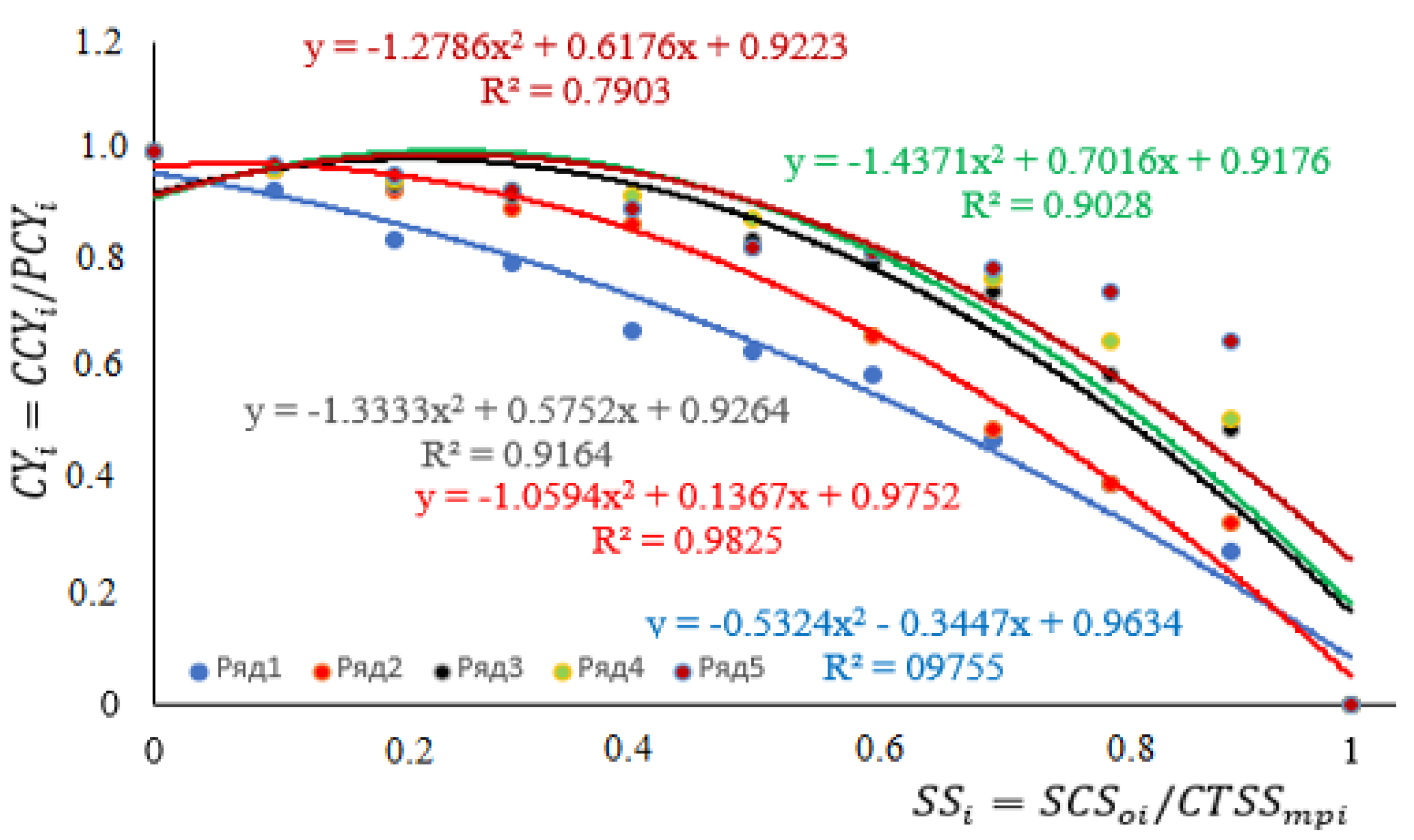
Plant Species	$$\begin{gathered} \mathbf{Equation} \mathbf{Parameters} \\ {\mathit{C}\mathit{Y}}_{\mathit{i}}\mathbf{=}\mathbf{(}\mathbf{-}\mathit{\alpha }·{{\mathit{S}\mathit{S}}_{\mathit{i}}}^2\mathbf{+}\mathit{b}\mathbf{·}{\mathit{S}\mathit{S}}_{\mathit{i}}\mathbf{)}\mathbf{+}\mathit{c} \end{gathered}$$			$\mathbf{Coefficient} \mathbf{of} \mathbf{Determination} \mathbf{\left(}{\mathit{R}}^2\mathbf{\right)}$	$\mathbf{Toxicity} \mathbf{Threshold} \mathbf{\left(}{\mathit{A}\mathit{l}}_{\mathit{t}\mathit{i}}\mathbf{\right)}$. mg/1000
	$\mathit{\alpha }$	$\mathit{b}$	$\mathit{c}$
Sugar beet	−0.5324	−0.3447	0.9634	0.9755	5.00
Alfalfa	−1.0694	0.1367	0.9752	0.9825	6.00
Red clover	−1.1744	0.4251	0.9309	0.8998	8.00
Buckwheat	−1.3333	0.5752	0.9264	0.9154	10.00
Corn	−1.4371	0.7061	0.9176	0.9076	10.00
Barley	−1.4371	0.7061	0.9176	0.9076	10.00
Forage beans	−1.4371	0.7061	0.9176	0.9076	10.00
Flax	−1.2786	0.6175	0.9223	0.7903	12.50
Oats	−1.4793	0.7561	0.9108	0.8945	18.00
Forage crops
$\mathrm{Cadmium} (\mathrm{C}d$)	−0.6379	−0.3150	0.9711	0.9964	0.3 мг/кг
$\mathrm{Lead} (\mathrm{P}b$)	−0.2016	−0.7104	0.9700	0.9859	0.5 мг/кг
$\mathrm{Zinc} (\mathrm{Z}n$)	−0.1955	−0.8098	0.9886	0.9922	100 мг/кг

).

Thus, the specific type of crop yield function describing the dynamics of soil salinity or mobile forms of heavy metals, developed using methods based on artificial intelligence and applied software like Microsoft Office, has enabled the generation of exponential, logarithmic, and polynomial equations with high correlation coefficient squared values ($R^2$). These equations can serve as tools to assess the convergence of the primary module, derived from solving differential balance equations with given initial and boundary conditions of the external environment.

The impact of soil salinity on the formation of agricultural crop yields and on the parameters of hydro-agro landscapes, as well as adjacent natural landscapes, has been proven by numerous studies in the Aral-Syrdarya water management basin, including in the Kyzylorda region. These studies have identified and examined various technologies for the effective use of salinized soils in agricultural production.

In the Kyzylorda region, where salinized soils and agro-landscapes prone to secondary salinization are widespread and where there is a shortage of water resources from the transboundary Syr Darya River, rice cultivation is practiced. This ensures simultaneous soil leaching and irrigation, contributing to the production of crops (

Table 3. The effect of soil salinity on rice field yields (1991–2023).

On Slightly Saline Soils (0.3–0.5%)			On Moderately Saline Soils (0.7–0.9%)			On Strongly Saline Soils (1.0–2.0%)
Yield	Difference in Yield Depending on the Predecessor		Yield	Difference in Yield Depending on the Predecessor		Yield	Difference in Yield Depending on the Predecessor
centners/ha	centners	centners/ha	centners	centners/ha	centners	%
1	2	3	4	5	6	7	8	9
On rotation with perennial grasses for 1–10 years
N60–90	P2O590–100	-	N90	P2O590–110	-	N120	P2O5125	-
57.8	-	-	53.1	-	-	48	-	-
Under the plasticity of perennial grass     Rotation for rice field 2–10 years
N90–120	P2O5110	-	N120	P2O5110	-	N130	P2O5130	-
53.1	4.7	8.1	47.8	5.3	10.0	41.8	6.2	13.0
On rice field 3–10 years						On rice field 3–10 years
N120	P2O5120	-	N120–150	P2O5120	-	N150	P2O5140	-
48.3	9.5	16.4	42.3	10.8	20.3	35.3	12.7	26.5

).

In rice crop rotation, rice is cultivated on the same field for up to three years, which corresponds to the step-by-step technology of developing saline soils over time in annual intervals.

Each stage of saline soil development corresponds to a specific state of soil salinity. Hydrogeochemical processes in the hydroagrolandscapes can be managed to promote soil desalinization in accordance with the technological scheme of gradual land reclamation, bringing soils from very saline to non-saline, which is a highly relevant task when incorporating saline landscapes into agricultural rotation.

As seen in Table 3, depending on the soil salinity and crop predecessors, rice yield changes in accordance with the mathematical model in the form of differential equations (15), which allow for the prediction of crop yields.

4. Discussion of Research Results

Based on the conducted studies, theoretical justification has been provided, and a conceptual model for managing crop yields on saline lands has been proposed. The distinctive features of this model are as follows:

Creation of a Research Database: Based on the collection, systematization, analysis, and evaluation of long-term experimental materials regarding the impact of soil salinity type and degree in various regions of Central Asia on crop yields, a research database has been established. This database helps identify mathematical and physical indicators of the relationship between crop yields and yield-forming factors [12,13,14,15,16,18].

Assessment of the Research Database’s Applicability: The possibility of using the research database as integral indicators for developing dynamic and linear correlation models of crop yields, depending on the type and degree of soil salinity, has been evaluated. The high coefficient of determination confirms the strong correlation between the function arguments and crop yields.

Development of Multidimensional and Unidimensional Mathematical Models: A system of multi-parameter and single-parameter mathematical models has been developed to characterize the process of crop yield formation under saline conditions, combined with agricultural techniques and irrigation technologies for agricultural land. These models serve as tools for managing natural resource use.

Mathematical Models for Yield Management: A system of mathematical models for managing crop yields under saline land conditions has been developed in the form of exponential, logarithmic, and polynomial equations. These models, with a given close relationship between the function arguments and crop yields, are integrated into digital technologies and can be used as the main tool for extending the research results to production areas.

5. Conclusions

Based on the created information resources and research data on the impact of soil salinity on the yield of agricultural crops in the salinized landscapes of agricultural use in Central Asia and Kazakhstan [54] from 1932 to 2020, and using the methodology of the materialistic theory of scientific knowledge, which includes experimentation, modeling, analysis, and synthesis, mathematical models have been developed for agricultural crop requirements under conditions of soil salinization. To verify the validity, reliability, and convergence of the obtained mathematical models, based on the solution of differential equations describing the studied process and the conditions that must satisfy the trajectory of crop yield changes depending on soil salinity in salinized agricultural landscapes, graph-analytic methods with Microsoft Office software were applied. As a result, exponential, logarithmic, and polynomial equations with high values of the coefficient of determination ($R^2$) were obtained as a consequence of the properties of the natural system, representing the nonlinearity of natural processes.

The main feature of the mathematical models for managing crop yields on saline lands is that, during their development, all empirical forms of experimental data are brought to a uniform dimension in the form of relative values, which ensures their universality. The accuracy and reliability of the strong relationships between the function arguments and crop yields, obtained in the form of exponential, logarithmic, and polynomial equations with high values of the coefficient of determination, are ensured by the use of digital technologies, which are one of the components of artificial intelligence.

The model reflecting the trends in agricultural crop yield changes depending on the soil salinity in salinized landscapes of agricultural use, which follow certain regularities or plant ecology laws, the most important of which are the law of equivalency or the substitutability of factors, the law of the limiting factor or Liebig’s minimum law («Liebig’s barrel»), the law of optimum or the law of cumulative factor action (Mitcherlich–Tineman–Baule law), the law of tolerance (Shelford’s law) [11], the principles of nonlinearity in natural processes, and the theory of allometry, which is a modification of the mathematical model by J. McElgunn and T. Lawrence [65], van Genuchten M. [66], Munns R., These M. [67], and Catherine M. et al. [68]. These allow determination under various assumptions of the quantitative and qualitative aspects of the studied process, providing valuable information necessary for analyzing the process in the territorial organization of agricultural production.

In conclusion, it should be noted that the developed system of mathematical models, which characterizes the crop yield formation process in saline soils of agricultural landscapes, allows for easy determination of the optimal conditions for various crops using available information resources. It serves as an effective tool for systemic analysis of anthropogenic activities aimed at transforming natural systems, within the framework of soft environmental management, combined with agricultural practices and production technologies. These models are tools for managing natural resource use, ensuring the construction of highly productive and environmentally sustainable agrolandscapes.

References

- FAO. Global Network on Integrated Soil Management for Sustain-Able Use of SaltAffected Soils; FAO: Rome, Italy, 2000; Available online: http://www.fao.org/ag/agl/agll/spush (accessed on 6 March 2025).
- Ghassemi, F.; Jakeman, A.J.; Nix, H.A. Salinisation of Land and Water Resources: Human Causes, Management and Case Studies; University of New South Wales Press: Sydney, Australia, 1995. [Google Scholar]
- Munns, R. Genes and salt tolerance: Bringing them together. New Phytol. 2005, 167, 645–663. [Google Scholar] [CrossRef]
- Pessarakli, M.; Szabolics, I. Soil salinity and sodicity as particular plant/crop stress factors. In Handbook of Plant and Crop Stress, 2nd ed.; Pessarakli, M., Ed.; Marcel Dekker: New York, NY, USA, 1999; pp. 1–16. [Google Scholar]
- FAO. FAO Statistical Year Book 2012, World Food and Agriculture; Food and Agriculture Organization of the United Nation: Rome, Italy, 2012; p. 366. Available online: http://www.fao.org/docrep/015/i2490e/i2490e00.htm (accessed on 6 March 2025).
- Kijne, J.W. Aral Sea Basin Initiative: Towards a Strategy for Sustainable Irrigated Agriculture with Feasible Nvestment in Drainage; Synthesis Report; IPTRID/FAO: Rome, Italy, 2005; p. 72. [Google Scholar]
- Tokbergenova, A.; Skorintseva, I.; Ryskeldiyeva, A.; Kaliyeva, D.; Salmurzauly, R.; Mussagaliyeva, A. Assessment of Anthropogenic Disturbances of Landscapes: West Kazakhstan Region. Sustainability 2025, 17, 573. [Google Scholar] [CrossRef]
- Mustafayev, Z.; Medeu, A.; Skorintseva, I.; Bassova, T.; Aldazhanova, G. Improvement of the methodology for the assessment of the agro-resource potential of agricultural landscapes. Sustainability 2024, 16, 419. [Google Scholar] [CrossRef]
- Qadir, M.; Noble, A.D.; Qureshi, A.S.; Gupta, R.K.; Yuldashev, T.; Karimov, A. Salt-induced land and water degradation in the Aral Sea basin: A challenge to sustainable agriculture in Central Asia. Nat. Resour. Forum 2009, 33, 134–149. [Google Scholar] [CrossRef]
- Khachaturyan, V.K.; Aydarov, I.P. Conceptual Approaches to Improving the Ecological and Meliorative Situation in the Aral Sea Basin. J. Land Reclam. Water Econ. 1991, 5–12. [Google Scholar]
- Reimers, N.F. Ecology. Theory, Laws, Rules, Principles, and Hypotheses; Russia Molodaya: Moscow, Russia, 1994; 367p. [Google Scholar]
- Kovda, V.A.; Mamayeva, P.Y. The Limits of Salt Toxicity in Soils of the Pakhte-Aral Region for Alfalfa and Cotton. Soil Sci. 1939, 80–98. [Google Scholar]
- Puruzyan, S.S. Influence of Soil Salinization on the Growth and Development of Corn. Soil Sci. 1959, 45–50. [Google Scholar]
- Rabochev, I.S.; Burdygina, V.S. Influence of Soil Solution Concentration on Cotton Yield. In A Collection of Articles; Ylym: Ashgabat, Turkmenistan, 1968; pp. 125–145. [Google Scholar]
- Tsyvilev, M.N. Influence of Solonetz on Southern Chernozem on Cereal Crop Yield. Soil Sci. 1975, 61–65. [Google Scholar]
- Gorbachyov, R.M. Development of Issues Related to the Efficiency of Hydro-Melioration in the Lower Amu Darya River. In Proceedings of the SANIRRI, Tashkent, Uzbekistan, 16–18 September 1980; pp. 54–68. [Google Scholar]
- Schmidt, S.M. Statistical Relationship Between Cotton Yield and Soil Salinization. In Collection of Scientific Papers of SANIRRI Principles of Regulating Reclamation Soil Regimes; Sugorish: Tashkent, Uzbekistan, 1982; Volume 166, pp. 132–143. [Google Scholar]
- Dukhony, V.A.; Umardzhanov, D. Methodology for Evaluating the Efficiency of Irrigation System Reconstruction. In Collection of Scientific Papers of SANIRRI/Improvement of Hydro-Reclamation Systems; Sugorish: Tashkent, Uzbekistan, 1982; Volume 167, pp. 41–80. [Google Scholar]
- Aidarov, I.P.; Pestov, L.F.; Korolyov, T.P. Influence of Soil Salinization Type and Degree on Crop Yield. In Collection of Scientific Papers of MGMI/Integrated Reclamation Regulation of Soil Processes; Moscow Hydrometeorological Institute: Moscow, Russia, 1982; pp. 120–131. [Google Scholar]
- Usmanov, A.U. Influence of Irrigation Water Quality on Crop Yield. Reclamation of Lands in the Lower Reaches of the Amu Darya River. In Proceedings of the SANIRRI; Sugorish: Tashkent, Uzbekistan, 1988; pp. 38–42. [Google Scholar]
- Nerpin, S.V.; Chudnovsky, A.F. Energy and Mass Exchange in the Plant-Soil-Air System; Gidrometeoizdat: Leningrad, Russia, 1975; 357p. [Google Scholar]
- Mitcherlikha, E.A. Soil Science; Foreign Literature: Moscow, Russia, 1957; 146p. [Google Scholar]
- Tang, J.; Riley, W.J. Finding Liebig’s law of the minimum. Ecol. Appl. 2021, 31, 02458. [Google Scholar] [CrossRef]
- Ramamoorthy, B.; Velayutham, M. The Law of Optimum and soil test-based fertiliser use for targeted yield of crops and soil fertility management for sustainable agriculture. Madras Agric. J. 2011, 98, 295–307. [Google Scholar]
- Mitscherlich, E.A.; Merrec, E. Eine guantitatire Stiekstoftanalyse für sehr geringe Mengen. Landwirtchaftliche Jahrbücher Z. Wiss. Landwirtsch. 1909, 7, 537–552. [Google Scholar]
- Griguletsky, V.G. Generalization of the law of action of growth factors and plant productivity of E.A. Mitscherlich. Oilseed Crops 2022, 2, 18–29. [Google Scholar] [CrossRef]
- Shelford, V.E. Some concepts of bioecology. Ecology 1931, 12, 455–467. [Google Scholar] [CrossRef]
- Ross, Y.K. Radiation Regime and Architecture of the Plant Cover; Gidrometeoizdat: Leningrad, Russia, 1975; 342p. [Google Scholar]
- Tooming, H.G. Solar Radiation and Crop Formation; Gidrometeoizdat: Leningrad, Russia, 1977; 200p. [Google Scholar]
- Moldau, H.A. Optimal Distribution of Assimilates Under Water Deficit (Mathematical Model). In Proceedings of the Academy of Sciences of the USSR, Biological Series; Consultants Bureau Enterprises: Moscow, Russia, 1975; Volume 24, pp. 3–9. [Google Scholar]
- Laisk, A.; Moldau, X.; Nielson, T.; Ross, Y.; Tooming, H. Modeling the Productivity Process of the Plant Cover. Bot. J. 1971, 56, 761–776. [Google Scholar]
- Sirotenko, O.D. Mathematical Modeling of the Water-Heat Regime and Productivity of Agroecosystems; Gidrometeoizdat: Leningrad, Russia, 1981; 167p. [Google Scholar]
- Khvalinsky, Y.A.; Sirotenko, O.D. Method for Calculating Photosynthesis of Agricultural Crops Based on Standard Meteorological Data. Proc. Inst. Meteorol. 1973, 3, 32–42. [Google Scholar]
- Polevoy, A.N.; Florya, L.V. Modeling of Agroclimatic Resources, Crop Yield Productivity, and Formation of Agricultural Crop Productivity. Hydrometeorol. Ecol. 2015, 31, 36–49. [Google Scholar]
- Mustafayev, Z.S.; Kozykeeva, A.T.; Zhidekulova, G.E. Model of Crop Productivity Formation in Hydroagrolandscape Systems. Int. Tech. Econ. J. 2017, 100–120. [Google Scholar]
- Paudel, D.; Boogaard, H.; de Wit, A.; Janssen, S.; Osinga, S.; Pylianidis, C.; Athanasiadis, I.N. Machine learning for large-scale crop yield forecasting. Agric. Syst. 2021, 187, 103016. [Google Scholar] [CrossRef]
- Ju, W.; Gao, P.; Zhou, Y.; Chen, J.M.; Chen, S.; Li, X. Prediction of summer grain crop yield with a process-based ecosystem model and remote sensing data for the northern area of the Jiangsu Province, China. Int. J. Remote Sens. 2010, 31, 1573–1587. [Google Scholar] [CrossRef]
- Kakabouki, I.; Roussis, I.; Mavroeidis, A.; Stavropoulos, P.; Kanatas, P.; Pantaleon, K.; Folina, A.; Beslemes, D.; Tigka, E. Effects of Zeolite Application and Inorganic Nitrogen Fertilization on Growth, Productivity, and Nitrogen and Water Use Efficiency of Maize (Zea mays L.) Cultivated Under Mediterranean Conditions. Sustainability 2025, 17, 2178. [Google Scholar] [CrossRef]
- Ullah Khan, F.; Zaman, F.; Qu, Y.; Wang, J.; Darmorakhtievich, O.H.; Wu, Q.; Fahad, S.; Du, F.; Xu, X. Long-Term Effects of Crop Treatments and Fertilization on Soil Stability and Nutrient Dynamics in the Loess Plateau: Implications for Soil Health and Productivity. Sustainability 2025, 17, 1014. [Google Scholar] [CrossRef]
- Fischetti, E.; Beni, C.; Santangelo, E.; Bascietto, M. Agroecology and Precision Agriculture as Combined Approaches to Increase Field-Scale Crop Resilience and Sustainability. Sustainability 2025, 17, 961. [Google Scholar] [CrossRef]
- de Freitas Cunha, R.L.; Silva, B.; Avegliano, P.B. Comprehensive Modeling Approach for Crop Yield Forecasts using AI-Based Methods and Crop Simulation Models. 2024. Available online: https://www.researchgate.net/publication/371727905 (accessed on 22 May 2024).
- Shabanov, V.V. Bioclimatic Justification of Reclamation; Gidrometeoizdat: Leningrad, Russia, 1975; pp. 342p. [Google Scholar]
- Misle, E. Allometric determination between mineral absorption and biomass in different cultivated species. Lat Am. J. Agric. Environ. Sci. 2006, 33, 67–71. [Google Scholar] [CrossRef]
- Misle, E. Simulating the accumulation of mineral nutrients by crops: An allometric proposal for fertigation. J. Plant Nutr. 2013, 36, 1327–1343. [Google Scholar] [CrossRef]
- Misle, E.; Garrido, E. Determination of crop nutrient accumulation under water or saline stress through an allometric model. In Proceedings of the 17 th International Symposium of the International Scientific Centre for Fertilizers (CIEC), Shenyang, China, 3–7 September 2018. [Google Scholar]
- Niklas, K.J. Plant Allometry: The Scaling of Form and Process; University of Chicago Press: Chicago, IL, USA, 1994; 395p. [Google Scholar]
- Enquist, B. Universal scaling in tree and vascular plant allometry: Toward a general quantitative theory linking plant form and function from cells to ecosystems. Tree Physiol. 2002, 22, 1045–1064. [Google Scholar] [CrossRef] [PubMed]
- Misle, E.; Kahlaoui, B. Nonlinear Allometric Equation for Crop Response to Soil Salinity. J. Stress Physiol. Biochem. 2015, 11, 49–63. [Google Scholar]
- Bloemberg, G.V.; Lugtenberg, B.J.J. Molecular basis of plant growth promotion and biocontrol by rhizobacteria. Curr. Opin. Plant Biol. 2001, 4, 343–350. [Google Scholar] [CrossRef]
- Bartels, D.; Sunkar, R. Drought and salt tolerance in plants. Crit. Rev. Plant Sci. 2005, 24, 23–58. [Google Scholar] [CrossRef]
- Manchanda, G.; Garg, N. Salinity and its effects on the functional biology of legumes. Acta Physiol. Plant 2008, 30, 595–618. [Google Scholar] [CrossRef]
- Dimkpa, C.; Weinand, T.; Asch, F. Plant– rhizobacteria interactions alleviate abiotic stress conditions. Plant Cell. Environ. 2009, 32, 1682–1694. [Google Scholar] [CrossRef]
- Bano, A.; Fatima, M. Salt tolerance in Zea mays (L). following inoculation with Rhizobium and Pseudomonas. Biol. Fertil. Soils 2009, 45, 405–413. [Google Scholar] [CrossRef]
- Yang, J.; Kloepper, J.W.; Ryu, C.M. Rhizosphere bacteria help plants tolerate abiotic stress. Trends Plant Sci. 2009, 14, 1–4. [Google Scholar] [CrossRef] [PubMed]
- Egamberdieva, D. Pseudomonas chlororaphis: A salt-tolerant bacterial inoculant for plant growth stimulation under saline soil conditions. Acta Physiol. Plant 2012, 34, 751–756. [Google Scholar] [CrossRef]
- Setia, R.; Gottschalk, P.; Smith, P.; Marschner, P.; Baldock, J.; Setia, D.; Smith, J. Soil salinity decreases global soil organic carbon stocks. Sci. Total Environ. 2013, 465, 267–272. [Google Scholar] [CrossRef]
- Panhwar, Q.A.; Naher, U.A.; Radziah, O.; Shamshuddin, J.; Mohd Razi, I. Bio-fertilizer, ground magnesium limestone and basalt applications may improve chemical properties of Malaysian acid sulfate soils and rice growth. Pedosphere 2014, 24, 827–835. [Google Scholar] [CrossRef]
- Qin, Y.; Druzhinina, I.S.; Pan, X.; Yuan, Z. Microbially mediated plant salt tolerance and microbiome-based solutions for saline agriculture. Biotechnol. Adv. 2016, 34, 1245–1259. [Google Scholar] [CrossRef]
- Yadav, A.N. Plant Microbiomes for Sustainable Agriculture: Current Research and Future Challenges; Yadav, A.N., Ed.; Springer International Publishing: Berlin/Heidelberg, Germany, 2020; pp. 475–482. [Google Scholar]
- Zamora Re, M.; Tomasek, A.; Hopkins, B.G.; Sullivan, D.; Brewer, L. Managing Salt-affected Soils for Crop Production (Revised 2022). Available online: https://extension.oregonstate.edu/catalog/pub/pnw-601-managing-salt-affected-soils-crop-production (accessed on 6 March 2025).
- Daba, A.W.; Qureshi, A.S. Review of Soil Salinity and Sodicity Challenges to Crop Production in the Lowland Irrigated Areas of Ethiopia and Its Management Strategies. Land 2021, 10, 1377. [Google Scholar] [CrossRef]
- Tukhtashev, B.B.; Norkulov, U.; EIzbasarov, B. The Role of Salt-Tolerant Crops in the Proper Use of Saline Soils. E3S Web Conf. 2024, 477, 00101. [Google Scholar] [CrossRef]
- Mishra, A.K.; Das, R.; George Kerry, R.; Biswal, B.; Sinha, T.; Sharma, S.; Arora, P.; Kumar, M. Promising management strategies to improve crop sustainability and to amend soil salinity. Front. Environ. Sci. 2023, 10, 962581. [Google Scholar] [CrossRef]
- Mustafayev, Z.S.; Abdeshev, K.B. Modeling of Soil Salinization and Desalinization Processes; LAP LAMBERT Academic Publishing: Chisinau, Moldova, 2023; 185p. [Google Scholar]
- McElgunn, J.D.; Lawrence, T. Salinity tolerance of Altai wild ryegrass and other forage grasses. Can. J. Plant Sci. 1973, 53, 303–307. [Google Scholar] [CrossRef]
- van Genuchten, M.T. Analyzing Crop Salt Tolerance Data: Model Description and User’s Manual; Research Report No. 120; U.S. Salinity Laboratory, USDA, ARS: Riverside, CA, USA, 1983. [Google Scholar]
- Munns, R.; Tester, M. Mechanisms of salinity tolerance. Annu. Rev. Plant Biol. 2008, 59, 651–681. [Google Scholar] [CrossRef] [PubMed]
- Grieve, C.M.; Grattan, S.R.; Maas, E.V. Plant salttolerance. In ASCE Manual and Reports on Engineering Practice No. 71 Agricultural Salinity Assessment and Management, 2nd ed.; Wallender, W.W., Tanji, K.K., Eds.; ASCE: Reston, VA, USA, 2012; Chapter 13; pp. 405–459. [Google Scholar]