Data-Driven Optimization of Construction and Demolition Waste Management: Pattern Recognition and Anomaly Detection

Abstract

Construction and Demolition Waste (CDW) forecasting is essential for sustainable waste management and circular economy objectives. Traditional prediction models often face limitations when dealing with small datasets and extreme variability. This study introduces a robust statistical framework that employs the median and Median Absolute Deviation (MAD), applied to standardized CDW indicators: tons per day (t day⁻¹) and tons per square meter (t m⁻²). The method enables the detection of statistical anomalies using a ±2·MAD threshold, increasing the model’s resilience to outliers and enhancing its predictive reliability. The analysis is based on a dataset of 16 construction and rehabilitation projects, carried out under consistent technical methodologies, operational practices, and centralized data collection protocols. The results show that median-based predictions offer greater stability than mean-based estimators, particularly in skewed datasets. The framework successfully identifies projects with significant deviations, supporting targeted audits, performance monitoring, and iterative model refinement. Although the current model focuses on the duration and area as predictors, future enhancements should incorporate additional contextual variables. Furthermore, embedding the median–MAD logic within machine learning architectures (e.g., LSTM, ARIMAX) could improve scalability and support real-time CDW monitoring. These findings contribute to the development of data-driven forecasting tools that are aligned with operational efficiency and circularity goals in the construction sector.

1. Introduction

Construction and Demolition Waste (CDW) management presents a significant environmental, economic, and operational challenge, primarily due to the construction sector’s intensive resource use, the substantial volume and heterogeneity of CDW generation, and the associated greenhouse gas emissions. Construction activities account for approximately 40% of natural resource use and generate 30–40% of urban waste globally, making CDW one of the largest waste streams worldwide [1,2]. The sector is also responsible for around 39% of energy-related carbon dioxide emissions, underscoring its critical role in mitigating climate change and related environmental concerns [3]. In particular, inadequate CDW management can contaminate soil and water in urban settings, demonstrating the pressing need for innovative and sustainable waste strategies. Addressing these challenges requires urgent measures, including the application of circular economy (CE) principles and the adoption of more advanced waste management approaches.

The CE offers a transformative framework to transition the construction sector from a “take–make–dispose” model to one that is centered on waste reduction, reuse, and recycling. Its core objective is to optimize resource efficiency and lower environmental impacts by fostering material circularity and decreasing the reliance on virgin resources. Notably, successful CE initiatives in regions like the European Union, aligned with the Green Deal, highlight the potential for enhancing sustainability in the construction industry [4,5,6]. For instance, employing secondary aggregates and selective demolition has reduced landfill use and improved resource efficiency [7,8]. Additional examples include strategies for recycling CDW into secondary aggregates, thereby minimizing both the use of virgin materials and the amount of waste that is sent to landfills [9]. Policies and technologies that support material circularity are therefore crucial to achieving a more sustainable construction sector [7,8].

The project duration and logistical factors are also influential in CDW generation. Extended project timelines often lead to the degradation of stored materials—particularly cement and plasterboard—and increase packaging waste, which can comprise up to 13% of total CDW in long-term efforts [10]. Meanwhile, proximity to recycling facilities affects recovery rates: long transport distances drive up costs and emissions, discouraging reuse or recycling in remote locations [9].

Indicators such as tons per square meter (t m⁻²), tons per capita per year (t person⁻¹ year⁻¹), and tons per day (t day⁻¹) are widely used to measure, parameterize, and compare CDW across various contexts [7]. These metrics capture differences based on the construction activity (new construction, demolition, refurbishment), the materials involved (e.g., concrete, wood, metals), and regional characteristics. For example, new construction projects typically generate 30–300 kg m⁻² of waste, while renovations can produce 200–1200 kg m⁻² [8,9]. In Sichuan, China, the amount of construction waste per unit of built area reached 0.550 t m⁻², demolition waste 1.3 t m⁻², and renovation waste 0.1 t m⁻² [11]. Likewise, the authors of Ref. [12] found a CDW generation rate of 0.069 t m⁻² for institutional non-residential projects, with specific values of 0.034 t m⁻² for concrete/masonry and 0.028 t m⁻² for wood [13].

Using the t person⁻¹ year⁻¹ indicator, Coelho and Brito [7] reported regional waste generation in Portugal ranging from 0.325 t person⁻¹ year⁻¹ to an anticipated 0.400 t person⁻¹ year⁻¹ over the next decade. Meanwhile, Germany accumulated 0.720 t person⁻¹ year⁻¹ and Ireland 0.162 t person⁻¹ year⁻¹ [7]. In Hong Kong, approximately 60 000 tons of CDW are produced daily, with 4400 tons being destined for landfills, which can hinge on the total project duration or working days [14]. These numbers highlight a pressing need for improved waste management.

Studies focusing on t m⁻² underscore the importance of material types. For instance, Ref. [8] documented 0.018–0.040 t m⁻² for new constructions and 0.401–0.840 t m⁻² for demolitions; among these, concrete may constitute up to 85% of the waste [8]. In Hanoi, Vietnam, Ref. [15] reported 0.079 t m⁻² for small construction sites and 1.030 t m⁻² for larger ones, with soil, concrete, and brick dominating the waste stream. Beyond area-based metrics, temporal indicators such as t day⁻¹ have proven valuable. Comparable approaches are found in [12,16], where effective working days were built into regression models, highlighting the critical role of project duration in forecasting CDW [12,14,16].

Numerous studies have employed such indicators to calibrate and predict CDW. For example, Ref. [17] constructed a multiple linear regression model incorporating dwelling numbers and total floor area, achieving R² values up to 0.99 in weight estimation but with potential volume deviations of ±38.48%. Similarly, Ref. [13] used regression models to estimate construction waste, discovering a mean generation rate of 0.151 m³/m² in Porto Alegre, Brazil, and reporting R² values of 0.81 and 0.91—indicative of strong predictive accuracy.

Despite progress in modeling (e.g., Support Vector Machine Regression or GM-SVR [11]), discrepancies persist between the forecasted and actual on-site CDW generation. In one example, Ref. [17] cited average deviations of ±0.75% by weight and ±10.28% by volume, with extreme outliers reaching ±38.48% (volume) and ±15.97% (weight). Likewise, Ref. [12] noted up to ±35% deviation for 79% of the dataset and highlighted how site-specific factors heavily influence the outcomes. The waste generation rate method and lifetime analyses are often limited by static datasets, failing to reflect real-world complexities, as [18] points out. Additionally, even buildings with comparable features may vary sixfold in waste generation, as shown in [13]. Consequently, more robust, context-specific techniques that incorporate real-time data and advanced statistical methods are essential [19].

The Median Absolute Deviation (MAD) method is an increasingly effective strategy for addressing forecasting errors and on-site variability in Construction and Demolition Waste (CDW) management. This robust statistical approach mitigates the influence of outliers, improving anomaly detection and enhancing the predictive accuracy in highly variable datasets [18,19,20,21,22]. For instance, Ref. [20] highlights the importance of advanced modeling techniques to manage CDW recycling volatility, a challenge that MAD is particularly well-suited to address. Similarly, research in Egypt emphasizes how site-specific outliers significantly impact CDW generation, reinforcing the need for robust statistical tools [21]. Unlike traditional dispersion measures, MAD calculates variability around the median, making it highly resistant to extreme values—a crucial advantage in construction projects that are characterized by unpredictability [23]. When integrated into hybrid or non-linear models such as GM-SVR—which combines Gray Model residuals with Support Vector Regression—MAD further enhances the predictive reliability by establishing adaptive confidence bands, reducing the risk of forecasting errors [11,24,25]. Improved forecasting accuracy leads to more efficient waste management decisions, better aligning predictive models with real-world conditions [26]. Additionally, MAD aids in identifying key drivers of large deviations, enabling the development of context-specific CDW management strategies that optimize resource allocation and minimize the environmental impact.

Notwithstanding the prevalence of indicators such as t m⁻² and t day⁻¹, discrepancies often remain between the projected and actual CDW generation on-site. While standard machine learning models and mean-based approaches capture broad waste patterns, they can falter when confronted with project-specific deviations stemming from material variability or local logistics. Consequently, this research integrates the median and MAD into predictive frameworks to systematically identify outliers, characterize waste generation patterns, and refine CDW projections. By improving the robustness and accuracy of these forecasts, the methodology contributes to more effective, data-driven CDW management practices that embrace CE principles and increase resource efficiency.

This study aims to develop a robust and data-efficient forecasting framework for CDW by applying the median and the Median Absolute Deviation (MAD) to two standardized indicators: average daily CDW generation (t day⁻¹) and CDW generation per intervention area (t m⁻²). The methodology improves the predictive reliability by enabling systematic anomaly detection and refined deviation assessment. By optimizing forecasting performance in small-sample, high-variability environments, the model supports informed decision-making in waste management practices that are aligned with circular economy (CE) principles.

In contrast to conventional models that are reliant on large datasets, multivariate regressions, or opaque machine learning techniques, this study introduces a statistically grounded and data-efficient approach. It applies robust estimators to standardized indicators across a set of construction and rehabilitation projects that were executed under consistent technical, operational, and data governance protocols. The combined use of the median and MAD supports outlier-resilient forecasting and enables anomaly detection through adaptive confidence intervals. This framework increases the statistical robustness in heterogeneous datasets and enables systematic performance monitoring, especially in data-constrained settings. It addresses a gap in the literature by offering a replicable method for anomaly-based forecasting, which is particularly relevant for organizations seeking to improve benchmarking and internal waste management through resilient, evidence-based tools.

2. Methods

This section presents the methodological framework that was used to analyze and predict Construction and Demolition Waste (CDW) generation. It includes the dataset, the definition of standardized indicators, the statistical techniques applied, and the anomaly detection method based on robust estimators.

2.1. Data Collection

Data on Construction and Demolition Waste (CDW) generation were collected from 16 projects, including 7 new construction and 9 rehabilitation interventions, all executed within a single metropolitan region in Portugal between 2017 and 2022. All projects were carried out by the same construction company, which employs approximately 250 members of staff and operates under a centralized data management system. This system ensured the application of uniform methodologies for construction execution, waste recording, and data handling.

Standardized construction techniques, machinery, and monitoring protocols were used across the entire sample. All projects were managed by the same technical team, using identical equipment and operational models. This high level of methodological consistency minimizes procedural variability and enhances the comparability of results, ensuring that observed differences in CDW generation primarily reflect intrinsic project characteristics—such as the duration, scale, and typology—rather than inconsistencies in data acquisition or site operations. Additionally, each project was categorized according to the construction type—namely, low-rise residential units (typically single-family dwellings or buildings up to two stories) and low-to-mid-rise buildings (including small apartment blocks or mixed-use structures with more complex structural requirements)—to support the subsequent interpretation of CDW variability.

Despite the internal coherence of the dataset, its relatively small size and localized nature (n = 16) limit the statistical generalizability of the findings. However, this methodological rigor offers a strong foundation for reliable intra-sample comparisons. Future studies should aim to expand the dataset by incorporating a broader range of construction typologies, systems, and geographic contexts, thereby improving the external validity and representativeness of the proposed forecasting model.

The CDW classification followed the European Waste List (EWL), as established by Commission Decision 2000/532/EC. This framework categorizes waste into 20 main categories and assigns specific six-digit codes to each type. The classification process in this study involved identifying waste generated across key construction phases—including raw material supply, transport, manufacturing, and on-site installation. Hazardous waste was isolated in accordance with European handling requirements.

To support consistent data analysis, five key variables were defined: (1) duration (days), representing the total project execution time; (2) intervention area (m²), indicating the built or affected surface; (3) CDW (t), capturing the mass of each waste type; (4) total CDW (t), denoting the overall quantity of waste that was generated per project. These parameters formed the quantitative basis for all subsequent analyses and indicator calculations.

2.2. Indicators

Two standardized indicators were established to allow for meaningful comparisons across projects of varying scales and typologies: (1) average daily waste generation (Equation (1)) and (2) waste generation per square meter of intervention area (Equation (2)).

These indicators normalize the waste output based on the project’s duration and size, respectively, allowing for more consistent assessment of the CDW intensity across heterogeneous cases.

$$\mathrm{CDWd} ={\displaystyle \frac{\mathrm{CDW}}{\mathrm{Duration} }}$$

(1)

$$\mathrm{CDWa}={\displaystyle \frac{\mathrm{CDW}}{\mathrm{Intervention} \mathrm{Area}}}$$

(2)

where

• CDWd (t day⁻¹): The average daily CDW generation.
• CDWa (t m⁻²): CDW per square meter of intervention area.
• CDW (t): The total amount of waste produced.
• Duration (days): The project’s execution time.
• Intervention Area (m²): The built or affected area.

These indicators provided the analytical foundation for the evaluation of central tendencies, predictive modeling, and anomaly detection that are described in subsequent sections. Each equation was applied directly using the project-specific data that were compiled during the data collection phase. Specifically, Equation (1) was used to calculate the average daily CDW generation by dividing the total observed waste by the project duration, while Equation (2) derived the waste intensity per intervention area. These operations were performed systematically across all 16 projects using a standardized spreadsheet environment, ensuring uniform computation and comparability of results.

2.3. Statistical Analysis

To examine the distributional characteristics of the indicators, both the mean (Equation (3)) and the median (Equations (4) and (5)) were calculated. While the mean reflects the overall central tendency, it is highly sensitive to extreme values. In contrast, the median provides a more robust estimate, particularly in the presence of skewed data or outliers.

$$\mathrm{Mean}={\displaystyle \frac{{{\displaystyle \sum }}_{\mathrm{i}=1}^{\mathrm{n}}{\mathrm{X}}_{\mathrm{i}}}{\mathrm{n}}}$$

(3)

where

• M (t day⁻¹ and t m⁻²): The mean of the observed values.
• X_i: The observed value (t day⁻¹ or t m⁻²).
• n: The total number of projects.

The median depends on whether the number of observations (n) is odd or even:

If n is odd, the following applies:

$$\mathrm{Median}={ \mathrm{X}}_{\left({\displaystyle \frac{\mathrm{n} +1}{2}}\right)}$$

(4)

If n is even, the following applies:

$$\mathrm{Median}={\displaystyle \frac{{\mathrm{X}}_{\left(\frac{\mathrm{n}}{2}\right)}+{ \mathrm{X}}_{\left(\frac{\mathrm{n}}{2}+1\right)}}{2}}$$

(5)

where

• Med. (t day⁻¹ or t m⁻²): The median of the observed values.
• X_i: The observed value (t day⁻¹ or t m⁻²).
• n: The number of projects.

A simplified predictive model was developed using robust estimators by multiplying the median value of each indicator by the corresponding project-specific variable. This generated two predicted values: CDW_pd, representing the total waste, estimated from the average daily generation rate (t day⁻¹), which was multiplied by the project duration in days (Equation (6)), and CDW_pa, representing the total waste, estimated from the waste intensity per square meter (t m⁻²), which was multiplied by the intervention area (Equation (7)).

$${\mathrm{CDW}}_{\mathrm{Pd} }=\mathrm{Median} \times \mathrm{Duration}$$

(6)

$${\mathrm{CDW}}_{\mathrm{Pa}}=\mathrm{Median} \times \mathrm{Intervention} \mathrm{Area}$$

(7)

where

• CDW_Pd (t): The predicted CDW based on average daily generation.
• CDW_Pa (t): The predicted CDW based on generation per unit of intervention area.
• Median (t day⁻¹ and t m⁻²): The median of the calculated indicator values (construction and rehabilitation).
• Duration (days): The duration of the project.
• Intervention Area (m²): The area of the project.

The reliability of the median-based forecasting model was evaluated by comparing the predicted and observed CDW values. Two complementary metrics were applied: absolute deviation (AD), which captures the direct difference between predicted and observed values, and relative deviation (RD), which expresses this difference as a percentage of the observed value (Equations (8) and (9)).

$$\mathrm{AD}={\mathrm{CDW}}_{\mathrm{p}}- \mathrm{CDW}$$

(8)

$$\mathrm{RD}={\displaystyle \frac{{\mathrm{CDW}}_{\mathrm{p}}- \mathrm{CDW}}{\mathrm{CDW}}}\times 100$$

(9)

where

• Absolute Deviation (AD, t day⁻¹ or t m⁻²): The direct difference between the predicted (CDW_p) and observed values (CDW).
• Relative Deviation (RD, %): The deviation expressed as a percentage of the observed value, enabling comparisons across projects of different scales.
• CDW_p (t day⁻¹ or t m⁻²): The predicted waste generation, calculated using Equations (6) and (7).
• CDW (t day⁻¹ or t m⁻²): The observed waste generation recorded for each project.

These metrics quantify discrepancies between predicted and observed values and serve as the basis for the anomaly detection procedures that are detailed in the following section. Equation (6) estimates the total CDW by multiplying the median daily generation rate (t day⁻¹) by the project duration (days), while Equation (7) applies the median per-area value (t m⁻²) to the project’s intervention area (m²). Absolute and relative deviations were then calculated using Equations (8) and (9), respectively. All equations were applied consistently across the dataset of 16 projects using a standardized spreadsheet-based framework to maintain methodological uniformity and analytical comparability.

2.4. Detection and Analysis of Anomalies and Patterns

Statistical anomalies between predicted and observed CDW values were identified using a robust detection method based on the Median Absolute Deviation (MAD). Rather than relying on arbitrary thresholds (e.g., ±10%), this approach defines confidence intervals that are grounded in the dataset’s internal variability.

The MAD was calculated as the median of the absolute deviations from the group-specific median, as shown in Equation (10).

$$\mathrm{MAD}=\mathrm{Median}\left(\left|\mathrm{Xi}-\mathrm{Med}.\left(\mathrm{X}\right)\right|\right)$$

(10)

where

• MAD (t day⁻¹ or t m⁻²): The Median Absolute Deviation, calculated as the median of the absolute differences between each observed value and the median of the group.
• X_i (t day⁻¹ or t m⁻²): The observed value for project i, either in absolute or relative terms depending on the analysis.

Based on this measure, upper and lower bounds for anomaly detection were computed using Equations (11) and (12). Values beyond these thresholds’ limits were flagged as anomalies.

$$\mathrm{Upper} \mathrm{Limit}=\mathrm{Median}+\left(\mathrm{k}\times \mathrm{MAD}\right)$$

(11)

$$\mathrm{Lower} \mathrm{Limit}=\mathrm{Median}-\left(\mathrm{k}\times \mathrm{MAD}\right)$$

(12)

where

• Upper Limit/Lower Limit (t day⁻¹ or t m⁻²): Thresholds defining the bounds of expected variability in CDW values.
• Median (t day⁻¹ or t m⁻²): The median of the absolute or relative deviations, calculated separately for construction and rehabilitation projects.
• k (–): A scale factor determining the width of the confidence interval; set to 2 in this study.
• MAD (t day⁻¹ or t m⁻²): The Median Absolute Deviation, calculated as the median of the absolute differences between each observed value and the median of the group (Equation (10)).

For anomaly detection, the scale factor k = 2, which follows empirical recommendations in the literature for balancing sensitivity and specificity in anomaly detection applications [22,23,24,25]. Lower values (e.g., k < 1.5) may lead to excessive false positives, while higher values (e.g., k > 3) can mask meaningful outliers. A sensitivity analysis of the parameter k was conducted and is further discussed in Section 3.3.

Moreover, the MAD was selected over other robust alternatives, such as the Interquartile Range (IQR), due to its superior ability to quantify dispersion symmetrically around the median. While the IQR identifies the middle 50% of the data, it does not yield a central measure that is suitable for defining symmetric intervals. In contrast, the MAD provides a direct measure of median-centered variability, making it particularly well suited for datasets with irregular or non-normal distributions.

The statistical thresholds derived through Equations (10)–(12) were applied to both the absolute and relative deviations that were calculated for each project. The MAD values and confidence bounds were determined separately for construction and rehabilitation projects to account for structural differences between the intervention types. Projects with deviations falling outside the calculated Median ± 2·MAD limits were flagged as anomalous. All calculations were performed using a standardized computational framework, ensuring consistent and reproducible application across the dataset.

3. Results and Discussion

This section presents the main findings on Construction and Demolition Waste (CDW) generation across a sample of 16 projects, including 7 new construction and 9 rehabilitation interventions. The analysis focuses on identifying key patterns, statistical anomalies, and the influence of project-specific characteristics such as the intervention area, project duration, and construction typology. Our CDW categorization follows the European Waste List (EWL), ensuring standardization and comparability across the dataset. To account for variations in project scale and execution time, two normalized indicators—waste generation per day (t day⁻¹) and per square meter (t m⁻²)—were utilized. Additionally, the use of the median and Median Absolute Deviation (MAD) provided a robust statistical foundation for both prediction and anomaly detection, making the method well suited to handle the heterogeneous nature of the dataset.

Despite the relatively limited sample size (n = 16), as detailed in Section 2.1, the methodological consistency across all projects strengthens the internal validity, ensuring that observed variations in CDW generation are attributed to project characteristics rather than procedural inconsistencies or data recording errors.

3.1. CDW Generation Patterns

Table 1. Summary of project characteristics, including intervention type, duration (days), intervention area (m²), and construction typology.

Type	Project	Duration (Days)	Intervention Area (m2)	Construction Type
Construction	C1	487	3580	Low-to-mid-rise building
	C2	548	5400	Low-rise residential unit
	C3	731	1321	Low-to-mid-rise building
	C4	243	3662	Low-rise residential unit
	C5	365	2581	Low-rise residential unit
	C6	731	4100	Low-rise residential unit
	C7	731	1413	Low-to-mid-rise building
Rehabilitation	R1	731	573	Low-to-mid-rise building
	R2	365	290	Low-rise residential unit
	R3	365	7000	Low-rise residential unit
	R4	545	1388	Low-to-mid-rise building
	R5	455	20,000	Low-rise residential unit
	R6	365	15,000	Low-rise residential unit
	R7	183	4000	Low-rise residential unit
	R8	183	15,000	Low-rise residential unit
	R9	365	621	Low-rise residential unit

presents an overview of each project’s key characteristics, including the intervention type, duration, intervention area, and construction typology. These variables are essential for understanding the sources of variability in CDW production and provide a structured basis for cross-case comparison.

Table 2. Classification and quantities of CDW generated per project according to European Waste List (EWL) codes. Total CDW represents the sum of all waste categories per project.

Type	Project	EWL	EWL Code Production (t)	CDW (t)
Construction	C1	17 04 05	16.76	113.58
		17 08 02	44.85
		17 09 04	51.97
	C2	17 01 07	141.59	5949.34
		17 02 01	9.76
		17 02 03	0.29
		17 04 05	2.57
		17 05 04	5734.25
		17 08 02	0.62
		17 09 04	57.72
		15 01 01	1.41
		15 01 02	0.68
		15 01 05	0.39
		19 12 01	0.08
	C3	17 04 05	2.4	24.76
		17 08 02	10.65
		17 09 04	11.71
	C4	17 09 04	7.92	7.92
	C5	17 09 04	4.36	4.36
	C6	17 09 04	3.94	3.94
	C7	17 02 01	4.42	449.46
		17 06 04	4.36
		17 08 02	6.96
		17 09 04	433.72
Rehabilitation	R1	17 01 07	2825.31	3692.56
		17 02 01	77.4
		17 04 05	62.95
		17 05 04	182.86
		17 09 04	541.08
		20 03 06	2.96
	R2	17 01 07	501.2	884.28
		17 02 01	23.1
		17 04 05	12.86
		17 04 07	0.32
		17 05 04	48.84
	R3	17 04 05	0.27	11.68
		17 09 04	11.415
	R4	17 01 03	10.38	37.03
	R5	17 01 07	13.42	163.95
	R6	17 01 07	58.48	79.57
	R7	17 01 03	4.08	29.14
	R8	17 01 07	17.24	17.68
	R9	17 01 03	17.12	23.29

presents the classification and quantities of CDW generated per project, categorized according to the European Waste List (EWL) codes. The total CDW per project was calculated as the sum of all waste categories reported, forming the observed variable that was used in both the modeling and anomaly detection processes. The table provides insights into the diversity of waste compositions and the recurrence of specific high-volume waste streams, such as excavation materials (EWL 17 05 04), structural demolition waste (EWL 17 01 07), and mixed construction waste (EWL 17 09 04).

The total CDW generated by each project displayed marked heterogeneity across the dataset. In construction projects, the values ranged from 3.94 tonnes (C6) to 5949.34 tonnes (C2). Although larger intervention areas generally resulted in greater waste volumes, this relationship was not strictly linear. For instance, Project C2, with an area of 5400 m², generated exceptionally high volumes due to substantial excavation activity, while C3, despite a long duration of 731 days, produced only 24.76 tonnes due to its limited demolition scope. Project C7, although relatively small in size (1413 m²), generated 449.46 tonnes of CDW, with a significant proportion consisting of mixed demolition waste.

Rehabilitation projects demonstrated even greater variability. Project R1 (573 m², 731 days) generated 3692.56 tonnes of CDW, primarily structural demolition debris and mixed waste, while R3, with a considerably larger area (7000 m²), produced just 11.68 tonnes. Notably, some large-area projects, such as R5 and R6 (20,000 m² and 15,000 m², respectively), exhibited comparatively modest CDW outputs (163.95 and 79.57 tonnes), further emphasizing that area alone is not a sufficient predictor of the waste volume. Conversely, R2, with only 290 m² of intervention, produced 884.28 tonnes, suggesting a highly demolition-intensive scope.

Across both categories, recurring waste types included excavation material (EWL 17 05 04), structural debris (EWL 17 01 07), and mixed construction waste (EWL 17 09 04). The predominance of these streams across project types reinforces their relevance in the design of waste reduction and valorization strategies.

The construction typology appears to influence waste patterns as well. Projects classified as low-to-mid-rise buildings (e.g., C1, C3, R1, R4) tended to exhibit both higher CDW quantities and greater heterogeneity in waste composition. Low-rise residential units, in contrast, generally produced lower and more homogeneous waste volumes. While the construction type was not explicitly modeled as a predictive variable, the observed trends suggest its potential as a relevant contextual factor in future analyses.

Based on the total waste, duration, and intervention area as listed in Table 2, the standardized indicators defined in Equations (1) and (2) were calculated for all 16 projects. These include average daily CDW generation (t day⁻¹) and CDW generation per square meter of intervention area (t m⁻²), which provide a normalized basis for comparing waste intensities across different project types and scales. The computed indicator values are summarized in

Table 3. Average daily CDW generation (t day⁻¹) and CDW generation per intervention area (t m⁻²) across construction and rehabilitation projects.

Type	Project	Duration (t Day −1)	Intervention Area (t m−2)
Construction	C1	0.23	0.03
	C2	10.85	1.10
	C3	0.03	0.02
	C4	0.03	0.0022
	C5	0.01	0.0017
	C6	0.0054	0.0010
	C7	0.61	0.31
Rehabilitation	R1	5.05	6.44
	R2	2.42	3.04
	R3	0.03	0.0017
	R4	0.06	0.02
	R5	0.36	0.0082
	R6	0.21	0.0053
	R7	0.15	0.0073
	R8	0.09	0.0012
	R9	0.06	0.037

.

Table 3 provides a quantitative overview of the CDW intensity across all projects, based on the two standardized indicators. Among the construction projects, the daily CDW generation ranged from 0.0054 to 10.85 t day⁻¹, while waste per square meter varied between 0.0010 and 1.10 t m⁻². Rehabilitation projects exhibited similarly wide dispersion, with daily values ranging from 0.06 to 5.05 t day⁻¹ and area-based values from 0.0012 to 6.44 t m⁻². These broad ranges reflect substantial differences in demolition methods, structural complexity, and the scope of material removal.

The project typology appears to significantly Influence the CDW Intensity. Projects classified as low-to-mid-rise buildings, such as C1, C3, R1, and R4, generally show higher values in at least one of the indicators, likely due to the structural complexity and material density that are typical of these constructions. In contrast, several low-rise residential units—including C6, R5, and R8—exhibited comparatively low CDW generation per area and per day, despite large intervention scales in some cases. This suggests that typology-related characteristics, such as construction techniques and material composition, may be more predictive of the CDW output than physical dimensions alone.

When compared to values reported in the literature, the observed construction indicators in this study (0.0017–0.31 t m⁻² or 1.7–310 kg m⁻²) generally fall within expected ranges. Exceptions at the upper end—most notably Project C2—can be attributed to intensive excavation activities [7,8,20]. The rehabilitation indicators (0.0053–6.44 t m⁻² or 5.3–6440 kg m⁻²) are likewise consistent with previous findings, particularly in cases involving structural refurbishment or partial demolition [7,8].

These results underscore the relevance of including contextual variables—such as the construction type, material typology, and site-specific operational conditions—into CDW forecasting models. They also highlight the limitations of relying solely on physical parameters such as the duration or intervention area. The use of standardized indicators not only improves comparability but also establishes a solid foundation for the statistical anomaly detection that is discussed in the following section.

3.2. Indicator Variability and Robustness Analysis

The statistical distribution of the standardized indicators presented in Table 3—average daily CDW generation (t day⁻¹) and CDW per square meter of intervention area (t m⁻²)—across the 16 projects was analyzed to assess the variability and determine the most appropriate measure of a central tendency for predictive applications. Given the heterogeneity in project duration, intervention area, and typology, these indicators enable consistent comparisons across interventions of different scales and scopes.

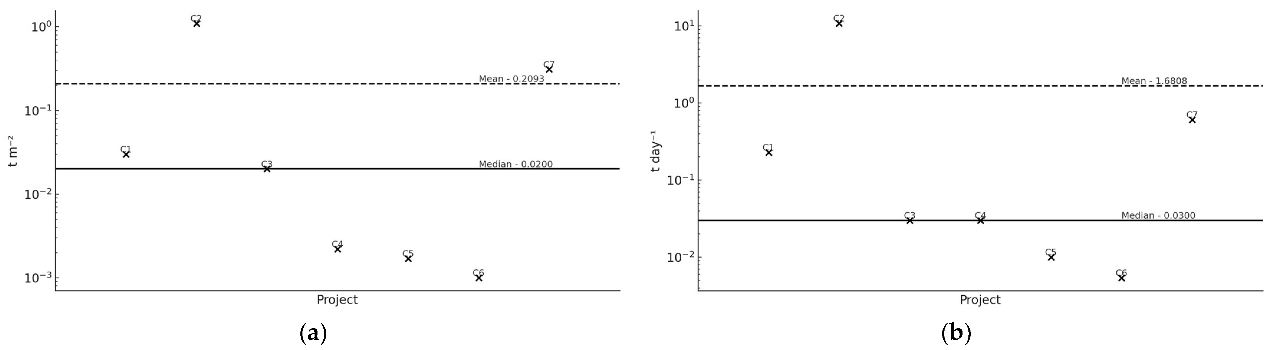
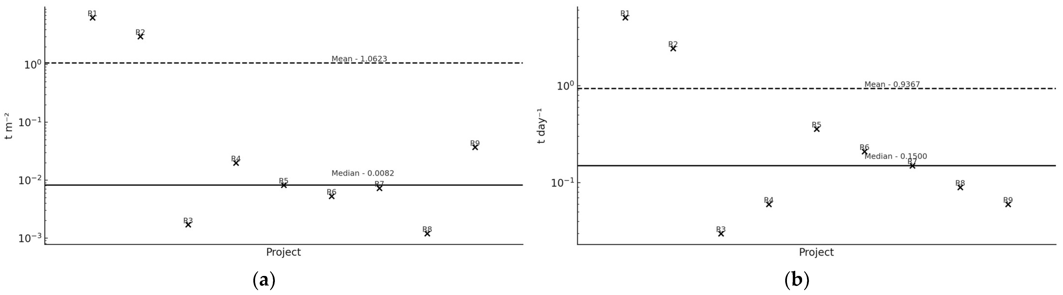
Figure 1 and Figure 2 display the distribution of both indicators across construction and rehabilitation projects, respectively. Each data point corresponds to a value listed in Table 3. The dashed and solid lines represent the group-specific mean and median, respectively, enabling direct visual comparison between these estimators.

As Figure 1 and Figure 2 illustrate, the mean is strongly influenced by high-output projects such as C2 and C7 (construction) and R1 and R2 (rehabilitation). These extreme values disproportionately elevate the mean, whereas the median remains stable and closer to the center of the distribution. This contrast highlights the robustness of the median and its superiority as a central tendency estimator for predictive purposes.

A quantitative analysis of the standardized indicators across all 16 projects reveals significant variability. The average daily CDW generation ranges from 0.0054 to 10.85 t day⁻¹, with a group mean of 1.31 t day⁻¹ and a median of 0.12 t day⁻¹. For CDW generation per square meter, the values range from 0.0010 to 6.44 t m⁻², with a mean of 0.69 t m⁻² and a median of 0.0141 t m⁻² (Figure 1 and Figure 2). These statistics highlight the dataset’s asymmetry and reinforce the divergence between the mean and the more robust median.

This divergence arises because the arithmetic mean incorporates all values equally, making it highly sensitive to extreme values. In scenarios involving CDW forecasting—where variations in material intensity, structural typology, and site conditions are significant—such robustness of the median is critical to prevent systemic overestimation.

The construction typology was further examined as a potential explanatory factor for the observed variability. The analysis of the results shows that low-to-mid-rise buildings present substantially higher CDW generation per unit area. For instance, construction projects C2 and C7 generated 1.10 and 0.31 t m⁻², respectively, whereas low-rise projects such as C5 and C6 generated only 0.0017 and 0.0010 t m⁻². Similarly, rehabilitation projects R1 and R4—both low-to-mid-rise buildings—produced 6.44 and 0.02 t m⁻², respectively, while low-rise units like R6 and R8 yielded just 0.0053 and 0.0012 t m⁻². These differences reflect the greater material intensity and structural complexity of low-to-mid-rise buildings. Such typological distinctions underscore the relevance of considering the construction type in predictive modeling, particularly when estimating CDW across diverse project portfolios.

Based on these distributional characteristics, the median was selected as the central estimator for predictive modeling. As detailed in Section 2.3, Equations (6) and (7) were used to compute predicted CDW values (CDWpd and CDWpa) for each project by multiplying the group-specific median indicator by the project’s duration or intervention area. The predicted values were then compared to the observed data (Table 3) using absolute deviation (AD; Equation (8)) and relative deviation (RD; Equation (9)). The full set of predicted values and their respective absolute and relative deviations from the observed data are presented in

Table 4. Predicted values of CDW generation per day (CDWpd) and per intervention area (CDWpa), including absolute and relative deviations (%) from the observed values.

		Duration			Intervention Area
Type	Project	CDWpd (t Day−1)	Absolute Deviation (t Day−1)	Relative Deviation (%)	CDWpa (t m−2)	Absolute Deviation (t m−2)	Relative Deviation (%)
Construction	C1	16.49	−97.09	−85.48	67.09	−46.49	−40.93
	C2	18.56	−5930.79	−99.69	101.2	−5848.15	−98.3
	C3	24.76	0.0	0.0	24.76	0.0	0.0
	C4	8.23	0.31	3.91	68.63	60.71	766.5
	C5	12.36	8.0	183.51	48.37	44.01	1009.38
	C6	24.76	20.82	528.32	76.84	72.9	1850.14
	C7	24.76	−424.7	−94.49	26.48	−422.98	−94.11
Rehabilitation	R1	116.4	−3576.16	−96.85	4.7	−3687.86	−99.87
	R2	58.12	−826.16	−93.43	2.38	−881.9	−99.73
	R3	58.12	46.44	397.57	57.38	45.7	391.23
	R4	86.78	49.76	134.39	11.38	−25.65	−69.27
	R5	72.45	−91.49	−55.81	163.95	0.0	0.0
	R6	58.12	−21.45	−26.96	122.96	43.39	54.53
	R7	29.14	0.0	0.0	32.79	3.65	12.52
	R8	29.14	11.47	64.87	122.96	105.28	595.67
	R9	58.12	34.83	149.52	5.09	−18.2	−78.15

.

The deviation analysis reveals three main patterns. First, negative deviations—as observed in C2 and R1—correspond to cases in which the actual CDW generation significantly exceeded the predicted values. These discrepancies are likely associated with atypical interventions involving substantial excavation or extensive structural demolition. Second, positive deviations, such as those identified in C5 and R9, reflect overestimations by the model and may be linked to projects that are characterized by limited material removal or a high reuse efficiency. Third, in certain projects (e.g., C3 and R5), the predicted and observed values matched exactly. This does not reflect overfitting, since no calibration or parameter tuning was applied. Rather, this coincidence is expected in small samples when project characteristics naturally align with the group median—especially under consistent operational conditions and limited variability.

Although the construction typology was not included as an explicit modeling variable, it may partially account for some of the observed deviations. For instance, C2, categorized as a low-rise residential unit, exhibited an unusually high CDW generation rate (10.85 t day⁻¹), suggesting the presence of intensive excavation that was atypical of its typology. Similarly, R1, a low-to-mid-rise building with a relatively small footprint (573 m²), generated an exceptionally high CDW per unit area (6.44 t m⁻²), likely due to comprehensive structural demolition. In contrast, C5 and R9—both low-rise residential projects—produced considerably less CDW than predicted, which is indicative of less invasive interventions. These cases highlight the potential influence of construction type on CDW generation and support its consideration in future modeling efforts.

The use of the median as a predictive baseline therefore provides a robust and resilient framework in the presence of outliers and skewed distributions. Its statistical stability enhances the reliability of CDW forecasting in heterogeneous datasets. The following section builds on this foundation by incorporating the Median Absolute Deviation (MAD) to formally establish thresholds for anomaly detection.

3.3. Statistical Detection of Anomalies and Patterns

Significant discrepancies between the predicted and observed CDW values were assessed using a robust anomaly detection method that combines the median with the Median Absolute Deviation (MAD). As detailed in Section 2.4, this method allows for the definition of upper and lower confidence limits that reflect the internal variability of the dataset and avoid the use of arbitrary thresholds—making it particularly suitable for small samples with high dispersion, as is common in construction-related studies.

Predicted CDW values were first calculated using Equations (6) and (7) by multiplying the group-specific median indicators by each project’s duration or intervention area. Discrepancies between predicted and observed values were then quantified using absolute deviation (Equation (8)) and relative deviation (Equation (9)).

The anomaly detection procedure involved two sequential steps. First, the MAD was computed as the median of the absolute deviations from the group median (Equation (10)). Second, upper and lower statistical bounds were established using Equations (11) and (12), which define the thresholds as the median ± k × MAD, with k = 2, following established empirical precedent [23,24,25]. Observations falling outside these bounds were flagged as statistical anomalies.

The resulting MAD values and the corresponding statistical thresholds for both construction and rehabilitation projects—and for both indicators (CDW per day and per intervention area)—are presented in

Table 5. MAD values and statistical limits for anomaly detection. MAD and upper and lower thresholds (±2 × MAD) for absolute and relative deviations in predicted CDW per day (t day⁻¹) and per intervention area (t m⁻²), by project type.

Type	Dimension	Deviation Type	MAD	Upper Limit	Lower Limit
Construction	Duration	Absolute Deviation	20.82	41.64	−41.64
		Relative Deviation (%)	94.49	188.98	−188.98
	Intervention Area	Absolute Deviation	60.71	121.42	−121.42
		Relative Deviation (%)	98.30	196.60	−196.60
Rehabilitation	Duration	Absolute Deviation	46.44	92.88	−92.88
		Relative Deviation (%)	93.43	186.86	−186.86
	Intervention Area	Absolute Deviation	43.39	86.78	−86.78
		Relative Deviation (%)	78.15	156.30	−156.30

. These values provide the basis for identifying significant absolute and relative deviations in predicted CDW generation. An analysis of the values presented in Table 5 revealed several notable anomalies. In particular, Project C2 exhibited a considerable underestimation (−5848.15 t m⁻²), while Project R2 showed a comparably large negative deviation (−5930.79 t day⁻¹). Several projects—including C1, C2, C7, R1, and R2—displayed substantial discrepancies across both temporal and spatial indicators.

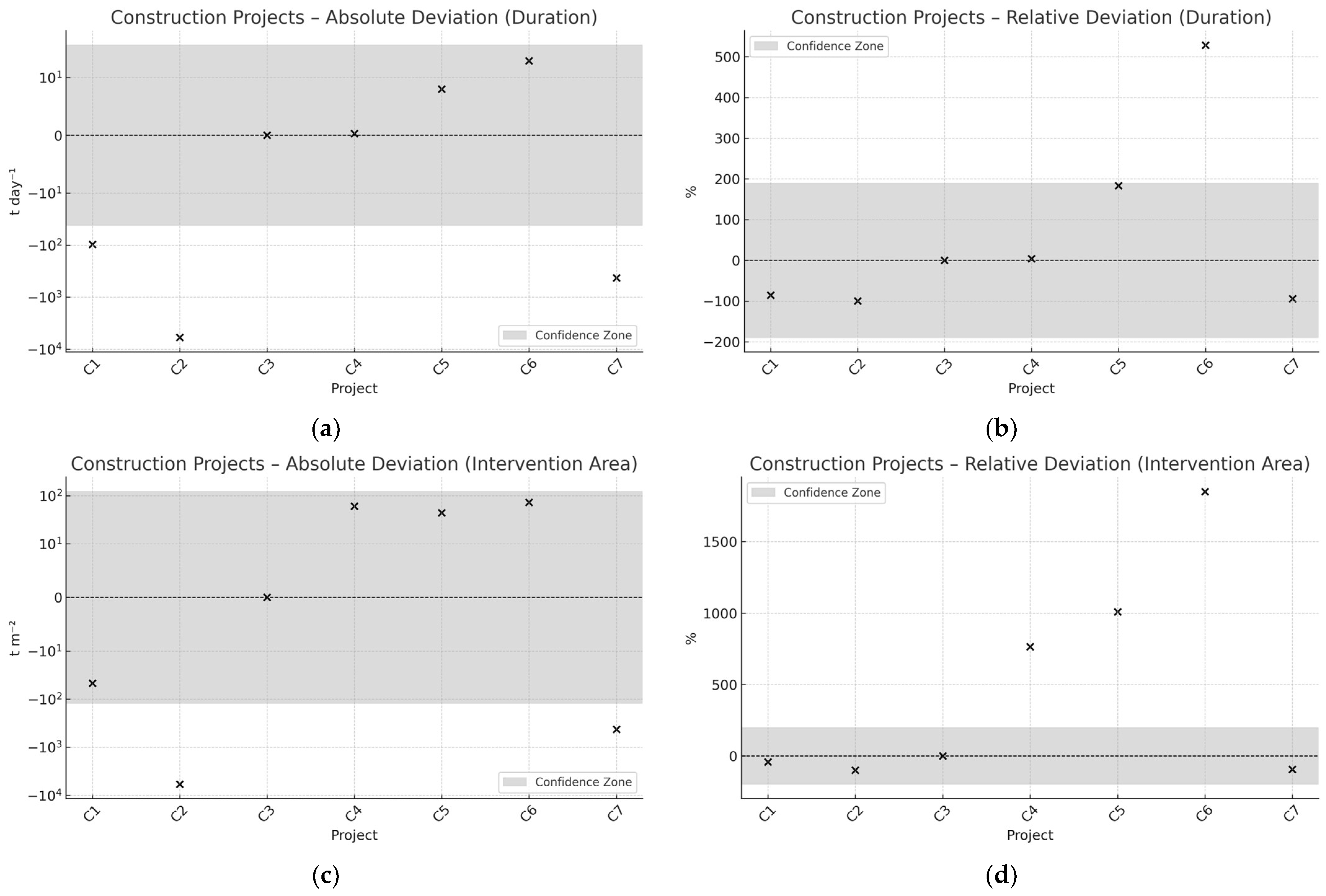
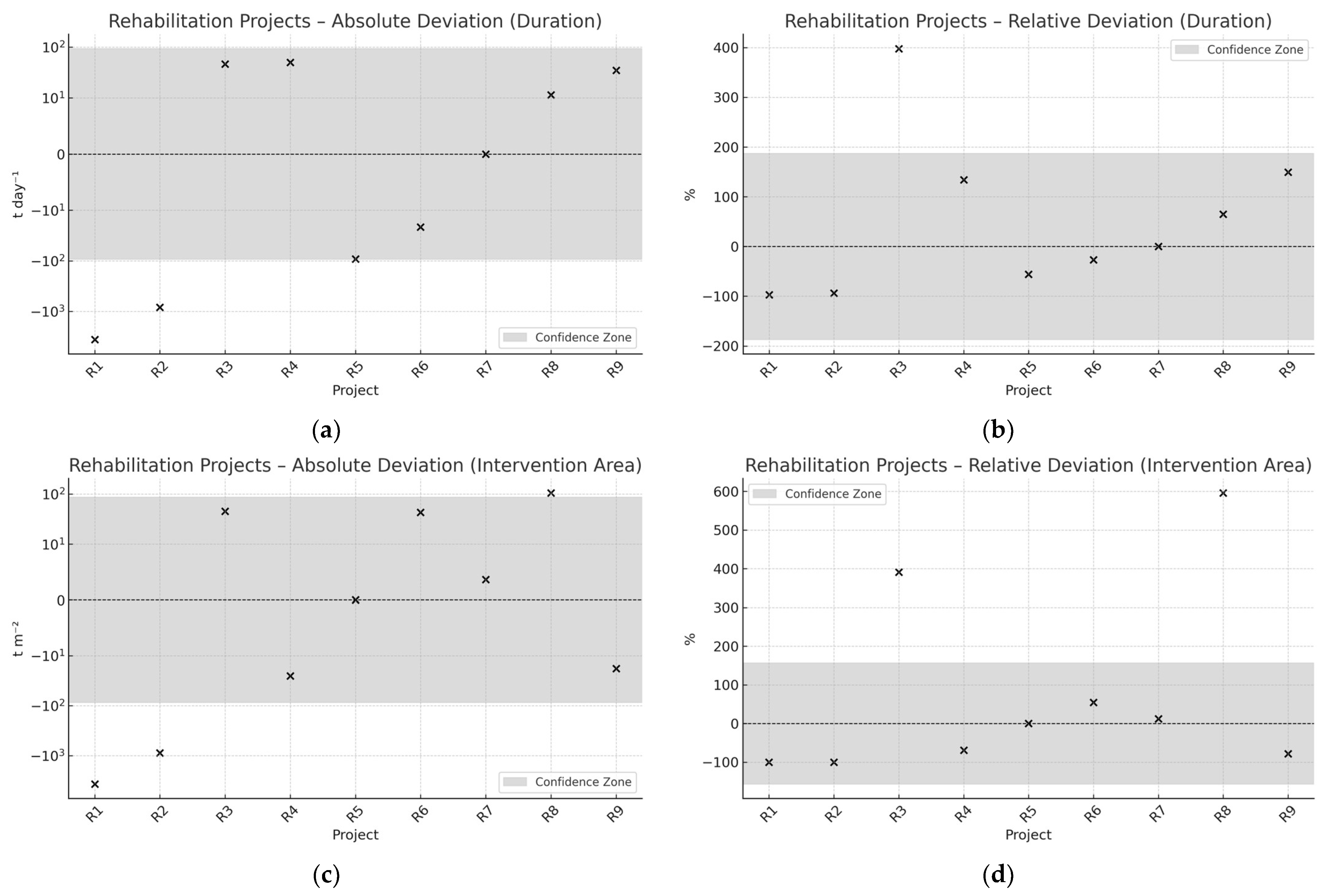
Complementing the statistical thresholds outlined in Table 5, the results were also plotted by project type and indicator category to support visual interpretation. Figure 3 displays the anomaly detection results for construction projects, while Figure 4 focuses on rehabilitation projects. Each figure contains four panels: (a) absolute deviation in CDW per day, (b) relative deviation in CDW per day, (c) absolute deviation per intervention area, and (d) relative deviation per intervention area.

Figure 3 and Figure 4 depict the deviation profiles for construction and rehabilitation projects, respectively, across four key dimensions: absolute and relative deviations in CDW generation per day (panels a and b) and per intervention area (panels c and d). The gray-shaded areas in each panel correspond to the statistical confidence bounds, calculated using the Median ± 2×MAD rule, with threshold values being summarized in Table 5.

In the absolute deviation plots (panels a and c), the vertical axis adopts a symmetric logarithmic (symlog) scale. This representation allows for balanced visualization of both negative and positive deviations while minimizing the influence of extreme values. Readability near zero is preserved, enabling a more faithful comparison across projects. In contrast, the relative deviation plots (panels b and d) are presented on a standard linear scale, as the distribution of values did not warrant transformation.

Projects C2, C7, R1, and R2 consistently fall outside the confidence bounds across all four indicators, indicating systemic deviations rather than isolated inconsistencies. These anomalies span both the spatial and temporal domains, suggesting persistent divergences from the expected CDW generation patterns. Project C2, for instance, a low-rise residential construction, recorded an observed output of 10.85 t day⁻¹, indicating substantial excavation or over-removal of materials. Similarly, R1, with a relatively small intervention area (573 m²), exhibited a high waste intensity of 6.44 t m⁻², most likely resulting from extensive structural demolition associated with vertical rehabilitation.

Some projects showed deviations in only one metric. Project C6 exceeded the spatial confidence bounds (Figure 3c,d) but remained within the temporal limits (Figure 3a,b), suggesting localized inefficiencies in material handling. Conversely, C5 and R3 exhibited lower-than-expected values across indicators, which may reflect optimized demolition practices or material reuse strategies.

The robustness of the anomaly detection approach was evaluated through a sensitivity analysis of the scaling parameter k in the Median ± k × MAD formulation, using values of 1.5, 2.0, and 3.0. Eight projects were flagged as outliers under k = 1.5 (C1, C2, C6, C7, R1, R2, R5, R8), while seven remained at k = 2.0. When the threshold was raised to k = 3.0, only four projects—C2, C7, R1, and R2—continued to fall outside the bounds. This persistence across all tested thresholds reinforces their classification as statistically robust anomalies, while the remaining cases appear to be sensitive to threshold variation and may reflect project-specific conditions rather than systematic discrepancies. The sensitivity analysis supports the choice of k = 2, as it provides the best balance between sensitivity and specificity, ensuring that meaningful anomalies are detected without generating excessive false positives.

By jointly analyzing the absolute and relative deviations in both the temporal and spatial dimensions, this two-axis diagnostic framework provides a nuanced interpretation of CDW generation performance. Single-axis anomalies may point to targeted operational inefficiencies, while multi-axis deviations suggest deeper inconsistencies that merit comprehensive evaluation in project planning, execution, or reporting practices.

3.4. Addressing Variability and Systemic Challenges

The standardization of waste generation indicators—specifically, average daily production (t day⁻¹) and production per square meter (t m⁻²)—strengthens the analytical coherence and comparability of the proposed forecasting framework. This foundation is further enhanced through the application of robust statistical methods based on the median and the Median Absolute Deviation (MAD), which together mitigate the influence of extreme values and enable consistent cross-project comparisons. The robustness of the adopted methodology contributes not only to a more consistent interpretation of CDW patterns across diverse project typologies but also provides a solid foundation for operational planning and regulatory compliance [13,14,20,27,28].

Compared to traditional predictive approaches—such as linear regression or artificial neural networks—the MAD-based methodology exhibits increased reliability in anomaly detection. Conventional models generally require large datasets for effective calibration [14], while the use of non-parametric statistics ensures resilience, even in contexts characterized by high variability and limited data availability. This makes the framework particularly suitable for professionals and public authorities managing CDW in small-scale or regionally confined project settings. As shown in Section 3.2 and Section 3.3, the median proves to be more stable than the mean in datasets with frequent outliers, further justifying its selection as the central estimator.

Despite its advantages, the current model formulation relies solely on two predictor variables: the project duration and intervention area. While these parameters are readily available and operationally relevant, they do not capture important contextual factors that can influence CDW generation. Variables such as the excavation depth, structural typology, construction techniques, or regional practices may significantly affect waste output, particularly in complex interventions. The absence of such variables is acknowledged as a limitation. To partially address this, the construction type was incorporated in Table 1 to distinguish between low-rise residential units and low-to-mid-rise buildings. Although not yet used as a formal predictor, this typological classification supports the interpretation of deviations and highlights pathways for future multivariate model refinement.

Beyond its forecasting accuracy, the MAD-based anomaly detection procedure provides a strategic advantage for targeted auditing and performance management. Projects exhibiting significant negative deviations—such as C2 and R2—can be prioritized for detailed review, while projects outperforming the predictions may reveal best practices that are worth generalizing. This dual functionality enhances decision-making and resource allocation. Integrating audit outcomes into the model’s recalibration establishes a dynamic learning loop, progressively refining its predictive accuracy and responsiveness. As organizations continue to apply the model across multiple projects, the accumulation of internal data leads to more representative median and MAD values. This progressive refinement increases forecast precision, narrows the expected deviation ranges, and improves anomaly detection, thereby enabling earlier and more effective intervention at the project level.

The implications of improved CDW forecasting extend beyond operational efficiency. Although not directly quantified in this study, reductions in Construction and Demolition Waste are closely associated with greenhouse gas (GHG) mitigation. More precise waste predictions help minimize unnecessary extraction, transport, and disposal of construction materials—activities that are closely linked to CO₂ emissions—thereby aligning with broader environmental and climate mitigation goals. Future extensions of this research could incorporate Life Cycle Assessment (LCA) data to quantify these environmental benefits more explicitly and reinforce the model’s contribution to sustainable construction practices [13,14,20,27,28,29,30,31].

Finally, incorporating advanced computational techniques may further improve the predictive capacity and scalability of the model. However, it is important to recognize that machine learning algorithms—such as LSTM networks or ARIMAX models—typically require large volumes of high-quality training data. This requirement may present a constraint, particularly for small or medium-sized construction enterprises with limited historical records. Nevertheless, in data-rich environments, such methods could complement the median–MAD approach by enabling more dynamic and adaptive forecasting systems. As audit processes become systematized and datasets grow, the model can evolve into a real-time monitoring system that is guided by key performance indicators (KPIs), enabling proactive waste management aligned with the principles of the circular economy—namely, material efficiency, emission reduction, and sustainable resource planning [29,30,31,32,33].

4. Conclusions

This study advances the predictive modeling of Construction and Demolition Waste (CDW) by applying standardized indicators—tons per day (t day⁻¹) and tons per intervention area (t m⁻²)—in conjunction with robust statistical estimators: the median and Median Absolute Deviation (MAD). This approach addresses key limitations of traditional forecasting methods by enhancing resilience to outliers and enabling statistically grounded anomaly detection.

The median demonstrated superior stability compared to the mean in datasets characterized by skewness and extreme values, offering a more reliable measure of central tendencies, as discussed in Section 3.2 and Section 3.3. The MAD enabled the construction of adaptive confidence intervals and the detection of statistical anomalies using a threshold of ±2·MAD. This framework allowed for the classification of projects with significant deviations—both positive and negative—thus supporting targeted interventions and audit prioritization.

The findings also revealed that generalized models fail to adequately capture the variability that is present in empirical CDW data. The forecast accuracy improves when predictions are anchored in project-specific parameters—such as the duration and intervention area—and refined through robust statistical thresholds, resulting in closer alignment with actual waste generation patterns.

From an operational standpoint, the MAD-based framework supports systematic benchmarking, informed auditing, and real-time performance feedback. As datasets expand, the reliability of the median and MAD as estimators is expected to increase, enabling the development of more sensitive and adaptive forecasting models. This positions the methodology as a foundation for scalable CDW monitoring systems that are aligned with circular economy principles.

Despite the methodological contributions, this study presents limitations that should be acknowledged clearly. Most notably, the small dataset (n = 16), while internally coherent and standardized, limits the representativeness and external validity of the findings. The lack of broader regional and typological diversity constrains the generalizability. Furthermore, the current framework is based on only two predictors—the intervention area and project duration—whereas other potentially influential variables (e.g., construction techniques, labor productivity, and transport logistics) remain unaccounted for. Including such variables could enhance the model’s predictive accuracy and contextual adaptability.

Future research should focus on consolidating and extending the applicability of the proposed framework by expanding the dataset and incorporating a broader range of construction typologies. The inclusion of additional contextual variables—such as structural systems, logistics constraints, or material typology—may further enhance the model’s generalizability and predictive robustness. Embedding the median–MAD logic within advanced machine learning architectures (e.g., LSTM, ARIMAX) also emerges as a promising path toward adaptive, real-time forecasting. Such developments would not only improve the responsiveness and accuracy of CDW prediction tools but also reinforce the construction sector’s alignment with broader goals of resource efficiency, regulatory compliance, and sustainable development.