The Impact of Customer-Centered Quality Management Systems on Profit and Satisfaction in Construction Companies

Abstract

In an increasingly competitive construction industry, quality management systems (QMSs) play a critical role in improving operational performance and customer satisfaction. Despite growing interest, limited research has examined how customer-oriented QMSs affect financial and non-financial outcomes in construction firms, particularly in emerging markets such as Kazakhstan. This study investigates the relationship between QMS implementation and company performance by analyzing data from 23 Kazakhstani construction companies. The methodology combines regression analysis, multivariate analysis, and k-means clustering to assess the impact of QMSs on sales volume, product profitability, quality management costs, and customer satisfaction. Regression analysis revealed that customer satisfaction (CSL), product profitability (PP), and economic efficiency of the QMS (EEQMS) have a statistically significant positive effect on sales volume (SV), while excessive quality costs (QMC) may negatively influence performance if not optimized. Cluster analysis further identified distinct groups of companies with varying levels of QMS effectiveness and profitability. This study offers empirical evidence on the financial value of customer-oriented QMSs in the construction sector. It contributes to the literature by highlighting performance drivers in QMS implementation and provides practical recommendations for managers and policymakers to improve quality strategies in similar regional contexts.

1. Introduction

In a globalized and competitive market, construction companies must optimize internal processes and prioritize customer needs to remain competitive.

One of the key tools for achieving these goals is the implementation of customer-centric quality management systems (hereinafter referred to as QMSs). Quality management systems, such as ISO 9001:2015 [1], play an important role in the construction industry by ensuring the quality of services and products, which in turn increases customer satisfaction and improves the financial performance of companies. According to Chen, J. and Li, Y., the implementation of customer-oriented approaches in quality management positively impacts company profitability by increasing customer trust and brand loyalty [2].

Kothai (2016) investigates the relationship between quality management systems and customer satisfaction in construction companies, emphasizing that effective quality practices lead to higher client trust and repeat business [3]. The study highlights that systematic quality management not only improves service delivery but also strengthens the company’s competitive position in the market [3].

Moreover, such companies are more resilient to market fluctuations and economic crises, as strong customer relationships create financial stability and flexibility. This approach is especially important for the construction sector, where high customer expectations and strict product quality requirements are key success factors.

Kazakhstan researchers also highlight the importance of quality management systems for construction companies in the country. For example, Zhuman Yeldar et al. found that companies implementing QMSs according to international standards, such as ISO 9001, demonstrate higher profitability and resource efficiency [4].

These standards help optimize business processes, reduce production costs, and improve quality control. Additionally, the researchers note that the implementation of QMSs in Kazakhstan construction companies leads to increased customer satisfaction, which contributes to greater demand and enhanced competitiveness in the domestic market [5]. Thus, this study aims to provide an in-depth analysis of the impact of customer-centric quality management systems on financial results and customer satisfaction in construction companies in Kazakhstan.

The main objective of this study is to identify the relationship between the implementation of QMSs and key performance indicators such as profitability, economic efficiency, and customer satisfaction. Drawing on both foreign and domestic research, this study seeks to propose new approaches to quality management in construction companies that can contribute to their long-term sustainability and success in the market.

2. Literature Review

2.1. Customer-Oriented QMS and Customer Satisfaction

Customer satisfaction has become a central theme in recent research on quality management systems (QMSs). Gonzalez and Rodriguez demonstrated that customer-focused QMS approaches significantly enhance customer satisfaction, which directly contributes to financial performance [6]. Chen and Li highlighted the strategic importance of aligning quality initiatives with customer needs as a pathway to process optimization and business success [7]. Similarly, Lopez and Parker and Talib et al. confirmed that customer-centered QMS practices are linked with higher service quality and organizational resilience [8,9].

Despite this agreement, the specific characteristics of the construction sector—such as project uniqueness, stakeholder complexity, and fluctuating client demands—require a more customized approach to QMSs. However, few studies have examined these dynamics in construction firms, which highlights the relevance of this study.

2.2. QMS and Operational Efficiency

Another important dimension in QMS research is operational efficiency. Peter and Hopkins found that a customer-centric QMS helps reduce operational costs by streamlining internal processes [10]. Studies by Martinez and Torres and Nguyen and Chang reported that standardization and communication improvements through QMSs reduce delays and production waste, enhancing profitability [11,12].

Mukhamedova and Karimov echoed these findings in the Kazakhstan context, where QMS implementation led to reduced defect rates and stronger performance metrics [13].

Earlier work by Zehir et al. and Kaynak supports these findings, emphasizing that integrated Total Quality Management (TQM) practices—particularly when embedded in a quality-driven culture—lead to sustained operational and financial benefits [14,15].

2.3. QMS Assessment and Continuous Improvement

Continuous assessment of QMS effectiveness has emerged as a key success factor. Wang and Li showed that companies using performance monitoring tools to evaluate QMSs achieved better financial results through bottleneck elimination [16]. Psomas and Jaca and Brown and Smith demonstrated that consistent feedback loops and real-time evaluation mechanisms contribute to better customer service and internal process optimization [17,18].

Regionally, Abdrasheva and Alibekova showed that QMS evaluation practices in Kazakhstan construction companies lead to sustainable competitive advantages, reinforcing the value of structured internal audits and performance reviews [19].

2.4. Digital and Sustainable QMS in Construction

Recent studies have linked QMSs not only to efficiency but also to sustainability and digital transformation. Lee and Han emphasized that digital QMS platforms improve transparency, allow real-time monitoring, and enhance managerial responsiveness in dynamic sectors like construction [20]. Rodríguez and Baeza discussed the integration of sustainable QMS practices in developing economies, noting that such systems help balance economic performance with environmental and social goals [21]. These studies strengthen the argument that QMS implementation is a strategic necessity in the Kazakhstan construction industry—not only for improving profitability but also for ensuring long-term sustainability and alignment with ESG (Environmental, Social, and Governance) principles.

2.5. Sectoral and Regional Focus in Transitional Economies

While the majority of the QMS literature focuses on manufacturing and service industries in developed countries, the construction sector in transitional economies presents unique challenges. Construction projects are complex, regulated, and capital-intensive, making them particularly sensitive to quality standards. Studies by Abdrasheva and Alibekova and Mukhamedova and Karimov underline the importance of contextualizing QMS implementation strategies based on local economic, cultural, and regulatory conditions [13,22]. This further underscores the importance of localized empirical research in countries like Kazakhstan.

Research Gap and Contribution

While the existing literature identifies strong links between QMSs, customer satisfaction, and efficiency, there remains a gap in applying these insights to the construction sector in emerging markets. This study addresses this gap by providing empirical evidence from 23 construction companies in Kazakhstan. It analyzes how a customer-oriented QMS influences financial outcomes, operational processes, and customer satisfaction. The findings contribute to both the academic literature and practical policymaking by offering actionable insights for improving QMS strategies in a developing-economy context.

Development of hypotheses. Based on the literature review, the following hypotheses have been identified for further empirical research:

H1: 

Implementation of a customer-oriented QMS has a positive effect on customer satisfaction.

H2: 

Optimization of business processes through a QMS leads to increased customer satisfaction and overall operational efficiency.

Review of the leading scientific directions for substantiating hypotheses. To substantiate the hypotheses, we review the leading scientific works of Peter, L., Hopkins, R., Nguyen, T., and Chang, H. [10,12], which demonstrate that the implementation of a QMS focused on process optimization reduces costs and increases profitability by improving operational efficiency.

Research by Wang, D. and Li, H. [16] and Brown, K. and Smith, J. [18] confirms that assessing the effectiveness of the QMS enables companies to identify weaknesses in a timely manner and optimize their processes.

Studies by Lopez, J. and Parker, S. [8] showed that process optimization through the QMS leads to improved product quality and increased customer satisfaction.

3. Research Methodology

The main objective of this study is to identify the relationships between key company performance indicators—such as sales volume, profitability, and customer satisfaction—and the effectiveness of quality management system (QMS) implementation. The methodological framework is based on proven quantitative techniques derived from both international and Kazakhstan empirical research.

3.1. Data Sources and Sampling Strategy

The analysis is based on data obtained from the official annual and financial reports of 23 construction companies operating in Kazakhstan. These reports are publicly available through corporate websites, government procurement databases, and financial disclosure platforms. They contain essential quantitative indicators required to assess QMS effectiveness.

A purposive sampling strategy was applied, selecting companies based on the availability of complete and comparable data for the most recent fiscal year. This approach ensures the reliability and objectivity of the data while minimizing the subjective biases typically associated with surveys or interviews.

To enhance data validity and reliability, all collected data were pre-standardized, verified for completeness and accuracy, and categorized into key indicator groups: process performance (PP), QMS implementation level (QMC and EEQMS), organizational characteristics (PO and SV), customer satisfaction (CSL), and others.

3.2. Sample Size Justification

To justify the adequacy of the sample size, a power analysis was conducted using standard parameters: medium effect size (0.5), significance level (α = 0.05), and statistical power (0.8). The results showed that a minimum of 21 observations is required under these conditions. Since this study includes data from 23 companies, the sample size is considered sufficient to ensure statistically valid conclusions. Figure 1 illustrates the outcome of the power analysis [23].

3.3. Analytical Methods

This study applies several quantitative methods to examine the relationship between QMS implementation and company performance:

−

Multivariate analysis was used to evaluate the economic efficiency of QMS implementation. Following the approach of Wang and Li, this method allows for assessing the impact of quality management costs on overall company profitability.

−

Regression analysis was employed to determine the relationship between product profitability and overall company profitability. This follows the methodology of Brown and Smith, who demonstrated a strong correlation between quality-related expenditures and company performance.

−

To assess customer satisfaction—a key indicator of QMS effectiveness—this study applies the methodology of Martinez and Torres, which utilizes structural equation modeling (SEM) to analyze the impact of product quality improvements on customer satisfaction and repeat purchases.

3.4. Cluster Analysis Approach

In addition to regression and multivariate analyses, cluster analysis was conducted to group companies by key performance indicators. This made it possible to assess differences in QMS implementation levels and classify companies based on variables such as sales volume, product profitability, overall profitability, and customer satisfaction.

The k-means clustering algorithm was selected due to its effectiveness with large numerical datasets and its ability to provide clearly interpretable results by defining distinct cluster centers. Hierarchical clustering methods were also considered but were found to be less robust to outliers and less scalable as data volume increases. Moreover, hierarchical clustering results tend to be more sensitive to the choice of distance metrics and linkage methods [24].

To determine the optimal number of clusters, the elbow method was used, and the stability of cluster structure was tested by repeatedly running the algorithm with different initial values (Ketchen, D. J., & Shook, C. L. [25]).

This approach follows the methodology of Lopez and Parker, who classified companies based on indicators such as quality management costs, product profitability, and overall profitability. The objective was to identify groups of companies that benefit the most from QMS implementation and those requiring process optimization.

3.5. Methodological Summary

The proposed methodological approach enables a comprehensive assessment of QMS effectiveness, integrating multiple analytical tools while accounting for the multidimensional nature of influencing factors. Contextual variables, such as company size and operational duration, were also considered, ensuring a well-rounded and reliable evaluation.

4. Analysis

In today’s highly competitive global environment, construction companies must go beyond improving product quality—they must actively prioritize customer satisfaction to ensure long-term success. The implementation of a customer-oriented quality management system (QMS) supports this by enhancing internal business processes, reducing inefficiencies, and increasing responsiveness to client needs. As a result, the QMS plays a crucial role not only in improving service quality but also in fostering customer loyalty and repeat business. Recent studies confirm this link between customer orientation and sustainable business outcomes. For instance, Adambekova et al. emphasize the importance of aligning quality and investment strategies with Environmental, Social, and Corporate Governance (ESG) principles to enhance stakeholder value and operational sustainability in the financial and construction sectors alike [26].

The following

Table 1. Matrix of the impact of a customer-oriented QMS on profit and customer satisfaction. Note. Compiled based on source [11].

Aspects/ Problems	Impact on Profit	Customer Satisfaction	Costs of Quality Management	Optimization of Business Processes
Customer focus in QMS	Impact of customer-oriented QMS on increasing profits through repeat orders and customer loyalty	Improving customer satisfaction by enhancing quality and meeting expectations	Costs of adapting the system to individual customer needs	Improving the efficiency of internal processes by optimizing interactions with customers
Economic efficiency of QMS	Increased product profitability through improved quality control and reduced defects	Increased customer trust and loyalty due to high product quality	High initial costs for QMS implementation, but long-term savings	Optimization of production processes and reduction in defects
Costs of QMS implementation and management	Short-term costs may reduce margins, but long-term payback may reduce defects and improve quality	Customers can appreciate the company’s efforts to improve quality, leading to long-term loyalty	High operating costs at the initial stage of implementation	Optimization of management costs and operational processes through standardization
Assessment of QMS effectiveness	Regular assessment of QMS effectiveness helps increase profitability by reducing costs and improving business processes	Increased customer satisfaction by continuous improvement in quality of services and products	The need for regular audits and monitoring, which increases operating costs	Continuous optimization of internal processes based on assessment results

outlines the research problems related to the impact of customer-oriented quality management systems on profits and customer satisfaction in construction companies.

Each cell of the Table 1 specifies issues and references pertinent studies.

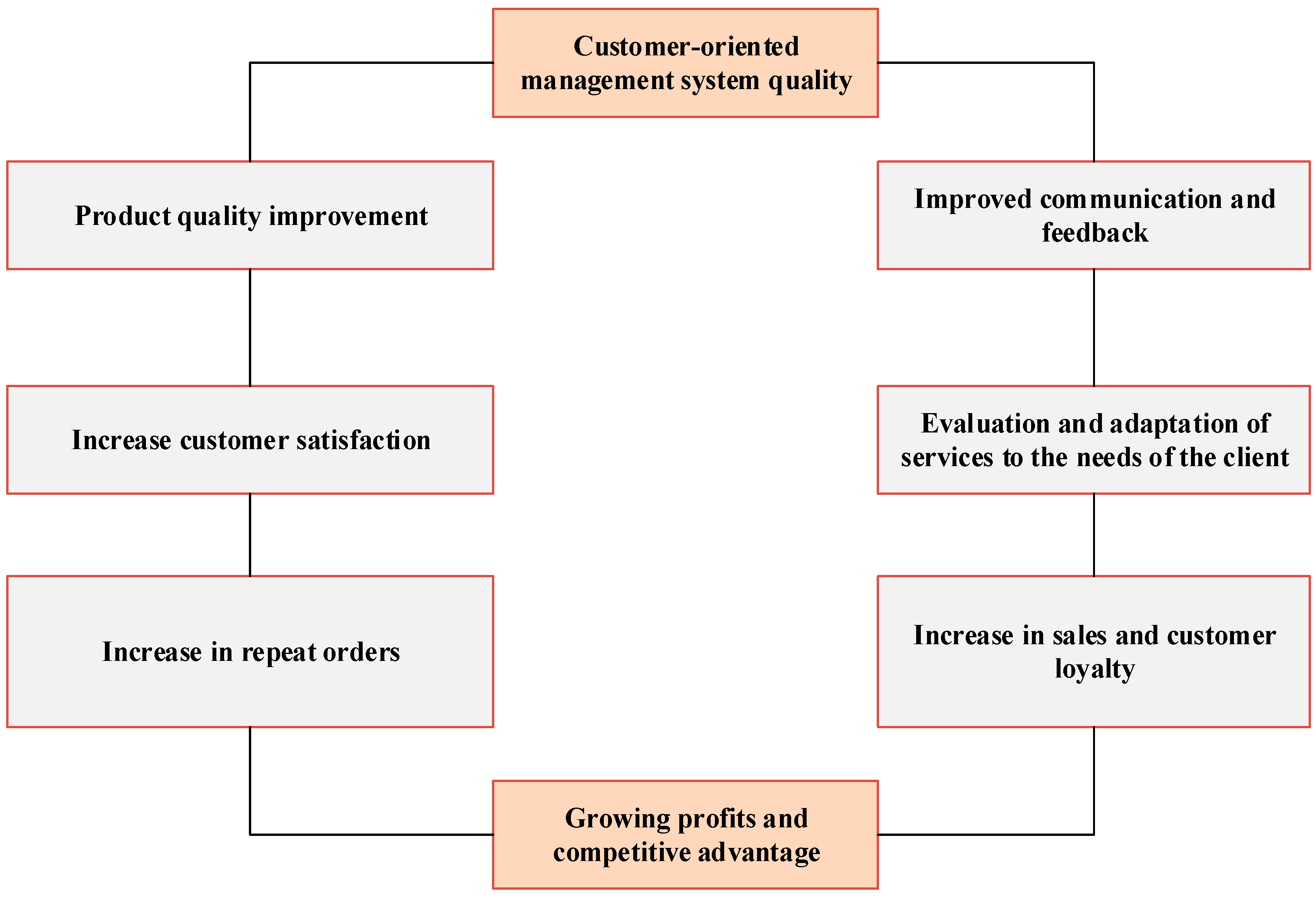
A customer-oriented quality management system (QMS) is a pivotal concept that aligns quality management processes and standards in construction companies with customer needs. This section explores how such systems affect productivity, customer satisfaction, and, ultimately, sales performance (Figure 2).

The implementation of a QMS significantly enhances product quality, which is a key driver of customer satisfaction. A customer-oriented QMS strengthens feedback mechanisms between companies and their clients, allowing for a clearer understanding of expectations and faster adaptation to changing customer requirements.

Improvements in product quality and feedback processes contribute to increased customer satisfaction. A well-implemented QMS enables companies to tailor their services and products more effectively to customer needs, thus fostering long-term relationships. Satisfied customers are more likely to place repeat orders, which stabilizes sales and improves financial performance.

As customer satisfaction and product quality improve, companies often experience growth in sales volumes and enhanced customer loyalty. These factors collectively contribute to increased profitability and a stronger competitive position in the market.

The regression analysis begins with the identification of key variables to evaluate how different factors influence sales performance in construction companies. The dependent variable in the model is sales volume (SV)—the core outcome being analyzed.

The independent variables include the following: economic efficiency of the QMS (EEQMS); quality management costs (QMCs); product profitability (PP); overall company profitability (OCP); customer satisfaction level (CSL); and company’s period of operation (PO).

EEQMS and QMC are expected to play a central role in shaping sales performance. While an efficiently implemented QMS can improve product quality and increase customer trust, excessive quality-related costs may have a negative short-term impact on financial outcomes if they do not result in tangible improvements.

Regression analysis is thus used to evaluate the trade-off between quality management costs and sales outcomes. The model also incorporates profitability indicators—PP and OCP—which reflect how effectively the company utilizes its resources to generate returns. Customer satisfaction (CSL) is also included, as it is a strong predictor of repeat purchases and long-term revenue stability.

Adding the company’s period of operation (PO) as a control variable allows for capturing the influence of company experience and market presence, which can significantly affect its ability to generate sales.

The regression analysis is based on data from 23 construction companies in Kazakhstan, collected for the year 2023. These companies represent diverse market segments—including residential, commercial, and industrial construction—and vary in size and regional location. This diversity enhances the generalizability and practical relevance of the findings.

Data were obtained from official financial and annual reports, which include both financial metrics (SV, QMC, PP, and OCP) and non-financial indicators (EEQMS and CSL). Utilizing data from a full calendar year ensures an accurate representation of current market conditions, including macroeconomic factors such as inflation, demand fluctuations in the construction sector, and material price volatility.

Thus, this dataset supports the identification of both general patterns and context-specific insights regarding the role of QMSs in enhancing company performance in the Kazakhstani construction industry.

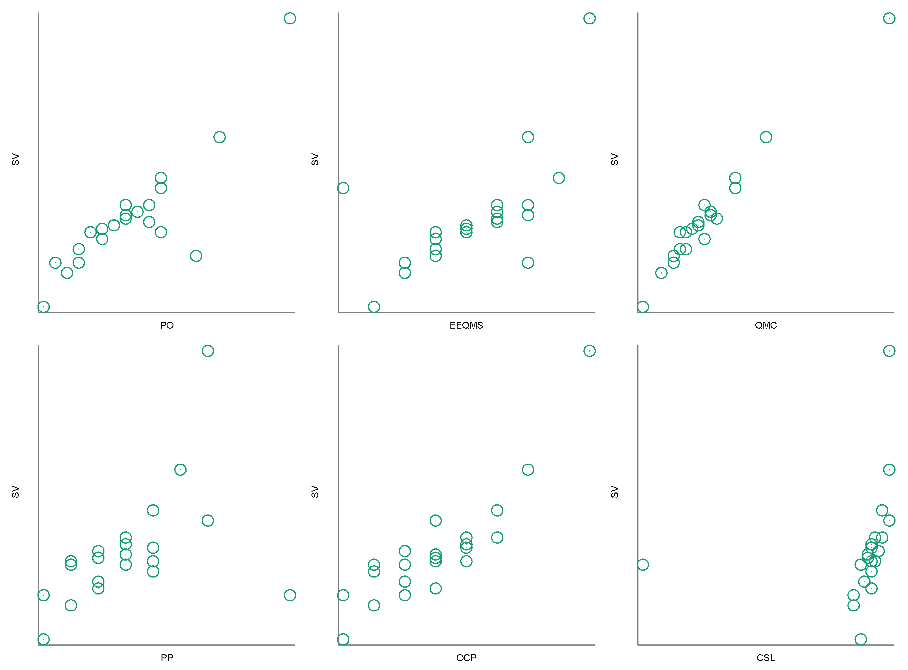
The Figure 3 demonstrates several positive correlations between key variables and the sales volume (SV) of construction companies. Notably, there is a moderate positive correlation between the company’s period of operation (PO) and its sales volume, indicating that firms with a longer market presence tend to achieve higher sales.

A weak but positive association is observed between the economic efficiency of the quality management system (EEQMS) and sales volume, suggesting that a more efficient QMS implementation may contribute to improved financial outcomes. Similarly, quality management costs (QMCs) show a positive, albeit weaker, correlation with sales, implying that increased investment in quality initiatives may lead to better performance, provided these costs are effectively managed.

Product profitability (PP) also exhibits a positive correlation with sales volume, although this relationship appears to be less pronounced. A stronger and more consistent relationship is identified between overall company profitability (OCP) and sales volume, highlighting the direct impact of broader financial performance on revenue generation.

Among all examined variables, customer satisfaction level (CSL) demonstrates the strongest positive correlation with sales volume, underscoring the critical role of client-oriented quality practices in driving repeat business and long-term financial success.

Overall, the correlation matrix provides valuable insights into the interrelationships among key performance indicators and justifies their inclusion in the regression model developed for this study.

Table 2. Model 1 OLS, using observations 1–23. Dependent variable: SV.

	Coefficient	Std. Error	t-Ratio	p-Value
const	−2.85727	0.729466	−3.917	0.0009	***
QMC	0.0172551	0.00110741	15.58	<0.0001	***
OCP	0.173853	0.0450511	3.859	0.0010	***
Mean dependent var	4.078261	S.D. dependent var		1.646196
Sum squared resid	1.076154	S.E. of regression		0.231965
R-squared	0.981950	Adjusted R-squared		0.980144
F(2, 20)	544.0018	p-value(F)		3.67 × 10−18
Log-likelihood	2.578570	Akaike criterion		0.842861
Schwarz criterion	4.249343	Hannan-Quinn		1.699581

White’s test for heteroskedasticity: null hypothesis: heteroskedasticity not present; test statistic: LM = 2.96435 with p-value = P(Chi-square(5) > 2.96435) = 0.705483. Test for normality of residual: null hypothesis: error is normally distributed; test statistic: Chi-square(2) = 6.00192 with p-value = 0.0497393. Chow test for structural break at observation 12: null hypothesis: no structural break; test statistic: F(3, 17) = 1.66062 with p-value = P(F(3, 17) > 1. *** p < 0.001.

presents the results of the statistical tests.

Constant (const): The coefficient is −2.85727, with a p-value of 0.0009, indicating that this variable is significant for the model.

QMCs (quality management costs): The coefficient is 0.0172551, with a p-value < 0.0001, suggesting a strong positive relationship between quality management costs and sales volumes. Each unit increase in QMC is associated with an increase in sales volumes (SV) by 0.017.

OCP (overall profitability of the company): The coefficient is 0.173853, with a p-value of 0.0010, indicating that an increase in the overall profitability of the company also has a significant positive impact on sales volumes. Each unit increase in OCP results in an increase in SV by 0.174.

General characteristics of the model: R-squared: 0.981950. The model explains 98.2% of the variation in the dependent variable (SV), indicating high explanatory power. Adjusted R-squared: 0.980144. The adjusted R-squared value also indicates a very high quality of the model, accounting for the number of predictors. F-statistic: 544.0018 with a p-value of 3.67 × 10⁻¹⁸, indicating that the model is overall significant.

White’s test for heteroscedasticity: p-value of 0.705483. Since the p-value is greater than 0.05, we conclude that there is no heteroscedasticity, implying that the variance of the residuals is constant.

White’s test for normality of residuals: p-value of 0.0497393. This value is close to the 0.05 threshold, suggesting a possible deviation from the normal distribution of residuals.

Chow test for structural break: p-value of 0.213026. There is no significant structural break at the 12th observed point, indicating the stability of the model.

Overall, the model demonstrates high explanatory power, with both predictors (QMC and OCP) having a significant positive effect on sales volumes. Diagnostic tests show the absence of heteroscedasticity and structural breaks.

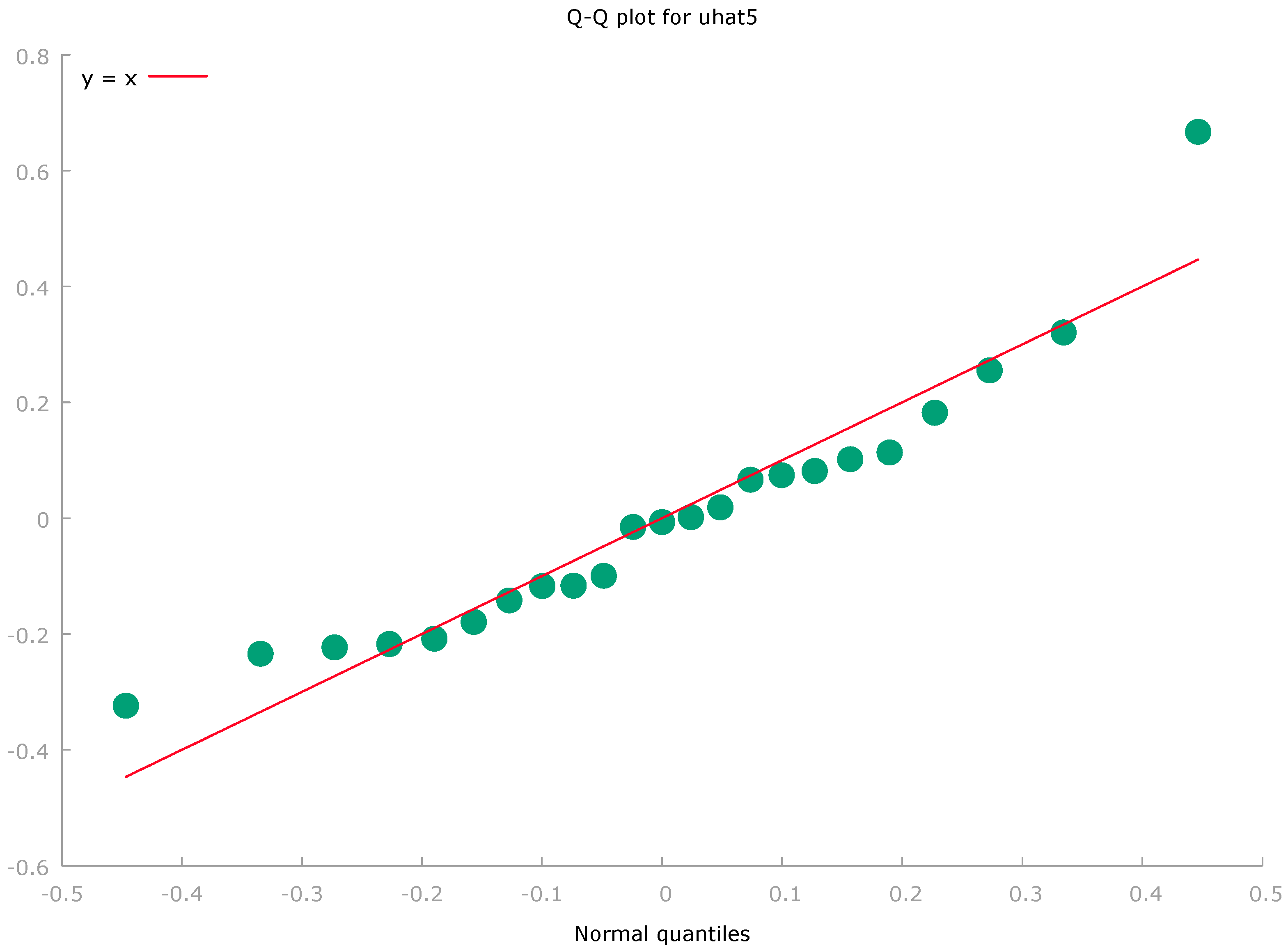
In this Figure 4, most of the points are close to the reference line, indicating that the residuals are normally distributed for the majority of the sample. However, an outlier is visible on the right side of the plot, which may suggest a slight deviation from normality in the tail of the distribution.

While the bulk of the residuals follow a normal distribution, the slight deviation observed in the upper right corner may indicate the presence of outliers. This observation is consistent with the result of the normality test, which reported a p-value of approximately 0.049, suggesting minor deviations from normality.

The confidence intervals for all coefficients do not include zero, confirming their statistical significance at the 95% confidence level (

Table 3. The 95% confidence intervals for the OLS model coefficients. t (20, 0.025) = 2.086.

	Coefficient	95 Confidence Interval
const	−2.85727	[−4.37891, −1.33563]
QMC	0.0172551	[0.0149451, 0.0195651]
OCP	0.173853	[0.0798783, 0.267828]

).

The accuracy of the model’s forecast was evaluated based on 23 observations.

Forecast evaluation statistics using 23 observations: Mean Error −8.5922 × 10⁻¹⁶; Root Mean Squared Error 0.21631; Mean Absolute Error 0.16375; Mean Percentage Error −0.76392; Mean Absolute Percentage Error 4.8736; Theil’s U1 0.024682; Bias Proportion, UM 1.686 × 10⁻²⁹; Regression Proportion, UR 5.1001 × 10⁻²⁸; Disturbance Proportion, UD 1.

Statistics are used to evaluate the accuracy of the model’s forecast based on 23 observations. They assess how well the model predicts the dependent variable values compared to the actual data.

Mean Error: −8.5922 × 10⁻¹⁶. The mean error is nearly zero, indicating that there is no forecast bias; the model does not systematically over- or under-predict values.

Root Mean Squared Error (RMSE): 0.21631. This value indicates good model accuracy, with relatively small deviations between the actual and predicted values.

Mean Absolute Error (MAE): 0.16375. This value suggests small deviations and indicates the model’s good predictive ability.

Mean Percentage Error (MPE): −0.76392. A negative value suggests that the model slightly systematically underestimates the predicted values compared to the actual ones.

Mean Absolute Percentage Error (MAPE): 4.8736%. This value indicates high accuracy of the model, with the average error being approximately 4.87%.

Theil’s U1 Index: 0.024682. This value indicates that the model outperforms the naive forecast and is accurate.

Bias Proportion (UM): 1.686 × 10⁻²⁹. A very small value indicates that the model has almost no systematic bias.

Regression Proportion (UR): 5.1001 × 10⁻²⁸. A very low value suggests a good fit between the forecast and the actual trend.

Disturbance Proportion (UD): 1. This value indicates that forecast errors are due solely to unaccounted random factors and not to systematic problems in the model.

Overall, the model demonstrates high forecast accuracy with minimal systematic deviations. The MAPE, RMSE, and Theil’s U1 index values indicate a good fit of the model to the actual data.

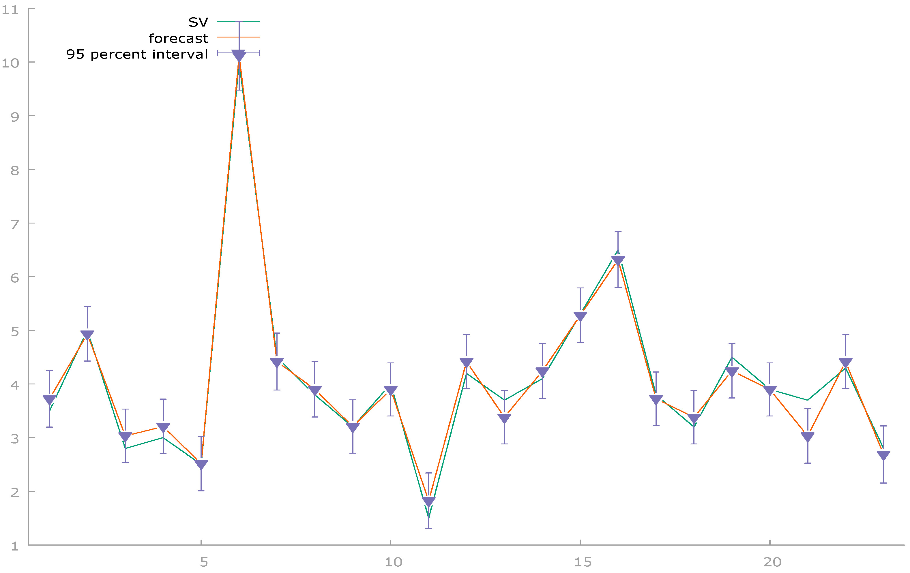
The model demonstrates a high degree of consistency between the forecasted and actual sales volumes. Most predicted values closely align with the observed data, while the narrow confidence intervals indicate strong predictive accuracy (Figure 5).

Regression analysis confirms that the constructed model possesses substantial explanatory power and is statistically significant for forecasting sales volumes in construction companies. The coefficients for quality management costs (QMCs) and overall company profitability (OCP) are statistically significant at the 95% confidence level (p < 0.001), highlighting their critical influence on sales performance.

The high values of R-squared (0.981950) and adjusted R-squared (0.980144) indicate that the model explains approximately 98% of the variation in the dependent variable, suggesting excellent model fit. Furthermore, low values of Root Mean Square Error (RMSE = 0.21631) and Mean Absolute Percentage Error (MAPE = 4.87%) further validate the model’s forecasting precision.

Diagnostic tests support the model’s robustness. White’s test indicates no presence of heteroscedasticity (p = 0.705483), while the Chow test confirms the absence of structural breaks (p = 0.213026). Although the residuals exhibit slight deviations from normality (p = 0.0497393), this does not materially affect the model’s overall reliability or validity.

Taken together, these results confirm the model’s high predictive power and stability, making it well suited for assessing the influence of quality management and profitability on sales volumes in the construction sector.

Building upon these findings, this study proceeds to segment companies through cluster analysis. While regression analysis quantifies relationships between variables, cluster analysis facilitates the identification of company groups based on shared characteristics, providing a deeper understanding of heterogeneity across firms.

The key variables selected for cluster analysis include overall company profitability (OCP), customer satisfaction level (CSL), economic efficiency of the QMS (EEQMS), and period of operation (PO). These indicators reflect both financial outcomes and the company’s ability to effectively implement quality management systems.

By applying k-means clustering, firms can be grouped according to similarity in these variables, enabling the identification of distinct strategic profiles in terms of quality management practices and customer orientation. This segmentation provides the basis for formulating targeted recommendations to enhance performance and competitiveness across company types.

The

Table 4. Number of observations in each cluster.

Cluster	1	2
	2	13
	3	8
Valid		23
Missing		0000

presents the inter-cluster distances obtained from the k-means cluster analysis, illustrating the differences between the identified clusters. The

Table 5. Distances between the terminal centers of clusters.

Cluster	1	2	3
1		11.535	18.813
2	11.535		7364
3	18.813	7364

largest distance is between Cluster 1 and Cluster 3 (18.813), indicating significant differences between them. Conversely, the smallest distance is between Cluster 2 and Cluster 3 (7.364), suggesting a greater similarity between these two clusters. This implies that Clusters 1 and 3 represent more distinct groups of companies, while Clusters 2 and 3 have more common characteristics.

The

Table 6. Final cluster centers.

	Cluster
	1	2	3
OCP	24.00	20.46	18.13
CSL	90.00	85.77	81.88
EEQMS	19.00	16.62	14.88
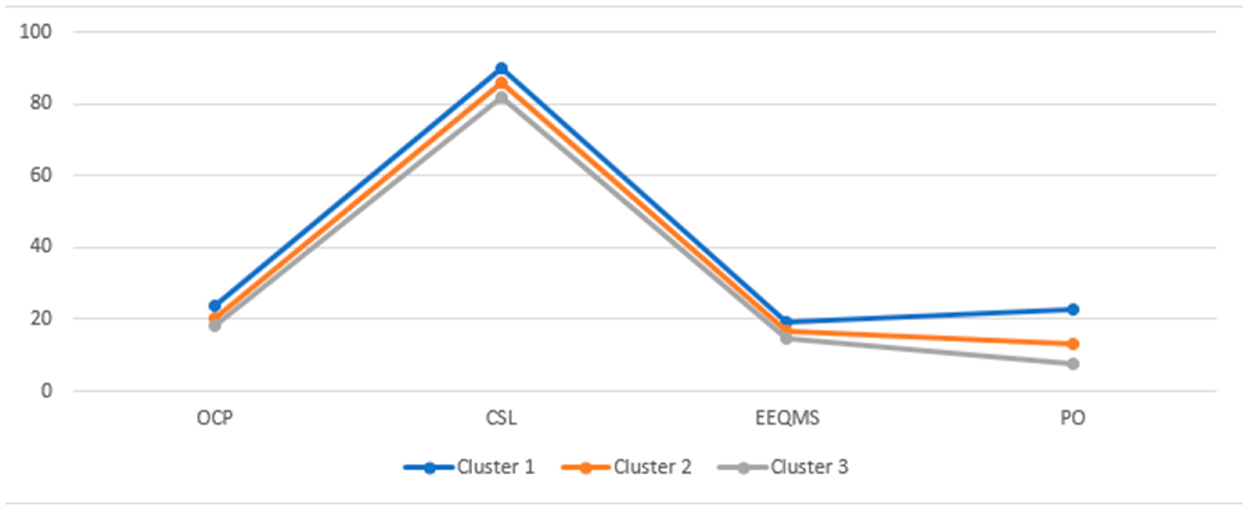
PO	23.00	13.15	7.63

shows the average values of key indicators for each cluster, including overall company profitability (OCP), customer satisfaction level (CSL), economic efficiency of the QMS (EEQMS), and the company’s period of operation (PO). Cluster 1 exhibits the highest values for all indicators: OCP = 24.00, CSL = 90.00, EEQMS = 19.00, and PO = 23.00. These high values may indicate that Cluster 1 comprises the most successful companies, characterized by a long period of operation and high customer satisfaction rates. Cluster 2 shows moderate values across all variables, whereas Cluster 3 has the lowest values, particularly for the period of operation (PO = 7.63) and economic efficiency (EEQMS = 14.88). This suggests that Cluster 3 includes companies with a lower efficiency and satisfaction level.

The Figure 6 presents the average values of key indicators (overall company profitability, customer satisfaction level, economic efficiency of QMS, and the company’s period of operation) for the three selected clusters.

The ANOVA table (

Table 7. Results of ANOVA (analysis of variance).

	Cluster		Error		F	Significance
	Mean Square	Degrees of Freedom	Mean Square	Degrees of Freedom
OCP	31.425	2	0.905	20	34.713	0.000
CSL	67.365	2	3759	20	17.920	0.000
EEQMS	15.981	2	1898	20	8421	0.002
PO	206.129	2	4978	20	41.405	0.000

F-test values should be used for descriptive purposes only, as the clusters are selected to maximize the differences between observations in different clusters. The observed significance levels are not adjusted for this selection, and therefore they cannot be used to test the hypothesis of equality of cluster means.

) presents the results of one-way analysis of variance for the four indicators (OCP, CSL, EEQMS, and PO) with respect to the clusters. All variables have high F-test values and significance levels (p-value of 0.000 or 0.002), indicating significant differences between clusters for each indicator.

For example, the F-test value for OCP (overall company profitability) is 34.713, reflecting strong differences between clusters. Similarly, the F-value for CSL (customer satisfaction level) is 17.920, and for PO (company’s period of operation) it is 41.405. It is important to note that the clusters were chosen to maximize the differences between observations.

The

Table 8. Clustering of construction companies.

CN	Distance
Cluster 1 Highly efficient companies
BI Group	3317
AlmatyStroy LLP	3317
Cluster 2 Average-performance companies
KazInzhenerin JSC	5325
Kazstroypodryad LLP	5186
AAEngineering Group LLP	3254
KulsarygaS LLP	3266
Intergasstroy LLP	2051
Set Stroy	2032
Exclusive Qurylys LLP	4487
Astana Construction LLP	2265
Aitkaz Group	4054
Nursat Engineering	3336
Elite Stroy Kazakhstan LLP	1099
KazkomplektStroy LLP	2892
IncomStroy LLP	1026
Cluster 3 Lower-performance companies
AlmatyStroy LLC	3929
Nur-Sat LLC	3767
Parus Construction	2165
RAMS Qazaqstan	1479
Smart Remont Ltd.	3419
EuroAsia Construction	1479
Grand Construction Group	1392
BestBuild Kazakhstan LLP	2861

https://ba.prg.kz/391010000-kostanay/010940002981-too-stroitelnaya-kompaniya-almatystroy/; https://kase.kz/ru/issuers/; https://bi.group/; https://www.kazstroypodryad.com/about; and https://ramsqz.com/ru/home (accessed on 21 January 2025).

provides information on the clustering of construction companies in Kazakhstan into three clusters based on various characteristics.

Cluster 1, which includes companies such as BI Group and AlmatyStroy LLP, demonstrates an average distance of 3.317. This indicates high efficiency, profitability, and customer satisfaction, characterizing these companies as market leaders with strong performance and stable operations.

Cluster 2 includes companies with average performance, such as JSC KazEngineering, Kazstroypodryad LLP, and Astana Construction LLP. The distances within this cluster range from 1.026 to 5.325, indicating variability in performance and satisfaction. Companies in this cluster exhibit balanced characteristics but have potential for improvement in specific aspects of their operations.

Cluster 3 encompasses companies with lower performance, including AlmatyStroy LLP, Smart Remont Ltd., and BestBuild Kazakhstan LLP. The average distances within this cluster range from 1.392 to 3.929. These companies may face challenges encountered in managing quality, profitability, and customer satisfaction, necessitating significant improvements to reach the performance levels of the companies in Clusters 1 and 2.

Table 9. Observation summary.

				CN	PO	SV	QMC
Observation cluster number	1	Total	Average		23.0000	8.2500	400.0000
		1		BI Group	26.00	10.00	500.00
		2		AlmatyStroy LLP	20.00	6.50	300.00
	2	Total	Average		13.1538	4.1615	200.0000
		1		KazInzhenerin JSC	15.00	5.00	250.00
		2		Kazstroypodryad LLP	18.00	3.00	150.00
		3		AAEngineering Group LLP	12.00	4.50	200.00
		4		KULSARYGAS LLP	10.00	3.80	180.00
		5		Intergasstroy LLP	14.00	4.00	190.00
		6		Set Stroy	12.00	4.20	210.00
		7		Exclusive Qurylys LLP	15.00	3.70	170.00
		8		Astana Construction LLP	12.00	4.10	220.00
		9		Aitkaz Group	15.00	5.30	250.00
		10		Nursat Engineering	10.00	3.80	180.00
		11		Elite Stroy Kazakhstan LLP	14.00	4.50	200.00
		12		KazkomplektStroy LLP	11.00	3.90	190.00
		13		IncomStroy LLP	13.00	4.30	210.00
	3	Total	Average		7.6250	2.9000	152.5000
		1		AlmatyStroy LLC	10.00	3.50	200.00
		2		Nur-Sat LLC	8.00	2.80	150.00
		3		Parus Construction	7.00	2.50	130.00
		4		RAMS Qazaqstan	8.00	3.20	160.00
		5		Smart Remont Ltd.	5.00	1.50	100.00
		6		EuroAsia Construction	8.00	3.20	170.00
		7		Grand Construction Group	9.00	3.70	160.00
		8		BestBuild Kazakhstan LLP	6.00	2.80	150.00
		Total	Average		12.0870	4.0783	200.8696

https://ba.prg.kz/391010000-kostanay/010940002981-too-stroitelnaya-kompaniya-almatystroy/; https://kase.kz/ru/issuers/; https://bi.group/; https://www.kazstroypodryad.com/about; and https://ramsqz.com/ru/home (accessed on 21 January 2025).

presents the characteristics of the identified clusters.

Cluster 1: Highly efficient companies in Cluster 1, such as BI Group and AlmatyStroy LLP, demonstrate superior performance across all parameters. The average period of operation (PO) in this cluster is 23 years, reflecting a long and stable market presence. Sales volumes (SV) average 8.25 million tenge, indicating a high level of market activity and success. Quality management costs (QMCs) are notably higher at 400, suggesting significant investment in quality management systems to maintain their high profitability and competitiveness. These companies are likely industry leaders, characterized by their robust performance and established market position.

Cluster 2: Medium-efficiency companies in Cluster 2 include companies such as JSC KazInzhenerin, Kazstroypodryad LLP, and Astana Construction LLP, which exhibit more balanced but moderate performance metrics. The average period of operation is 13.15 years, indicating a stable, though shorter, market presence compared to Cluster 1. Average sales volumes are 4.16 million tenge, lower than those in Cluster 1. Quality management costs in this cluster are 200, representing the average for the sample. Companies in this cluster have potential for growth and can enhance their efficiency by optimizing quality management costs and increasing sales volumes.

Cluster 3: Low-performance companies in Cluster 3 comprise companies such as AlmatyStroy LLC, Parus Construction, and Smart Remont Ltd., which exhibit the lowest performance indicators. The average period of operation is 7.63 years, indicating a shorter market presence compared to the other clusters. Sales volumes average 2.90 million tenge, significantly lower than in the other clusters, suggesting lower market activity and efficiency. Quality management costs average 152.5, reflecting minimal investment in quality management systems and potentially lower product or service quality. Companies in this cluster are likely to face challenges in improving profitability and customer satisfaction.

Summary: Cluster 1 represents the top-performing companies with high sales volumes, extensive operational histories, and significant investments in quality management. Cluster 2 includes mid-level companies that have been in the market longer than the companies in Cluster 3, but still fall short of the leaders. Cluster 3 contains companies with the lowest indicators for all variables, pointing to potential issues in quality management strategies and overall business development.

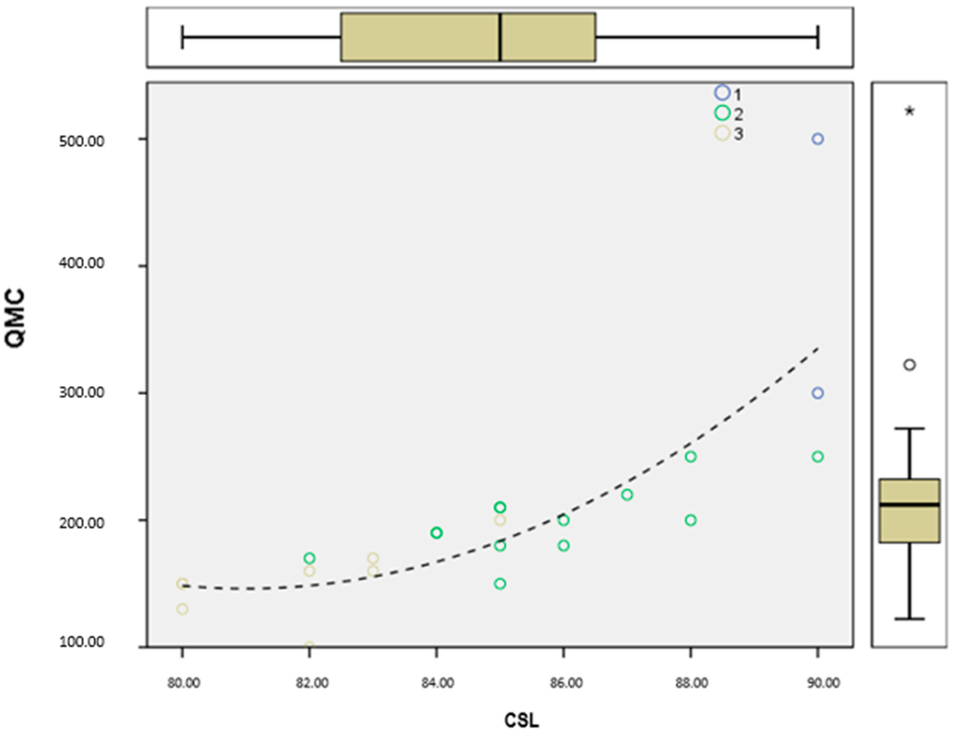
The Figure 7 illustrates the relationship between quality management costs (QMCs) and customer satisfaction level (CSL) for companies grouped into three clusters. Different colors represent different clusters: blue for Cluster 1, green for Cluster 2, and yellow for Cluster 3. There is a positive relationship between quality management costs and customer satisfaction level: as QMC increases, the CSL also rises. This is confirmed by the trend curve (dashed line), which shows an increase in QMC alongside an increase in CSL.

The figure also presents the distribution of values across the cluster using box plots, which depict data spread and highlight individual outliers, representing specific companies.

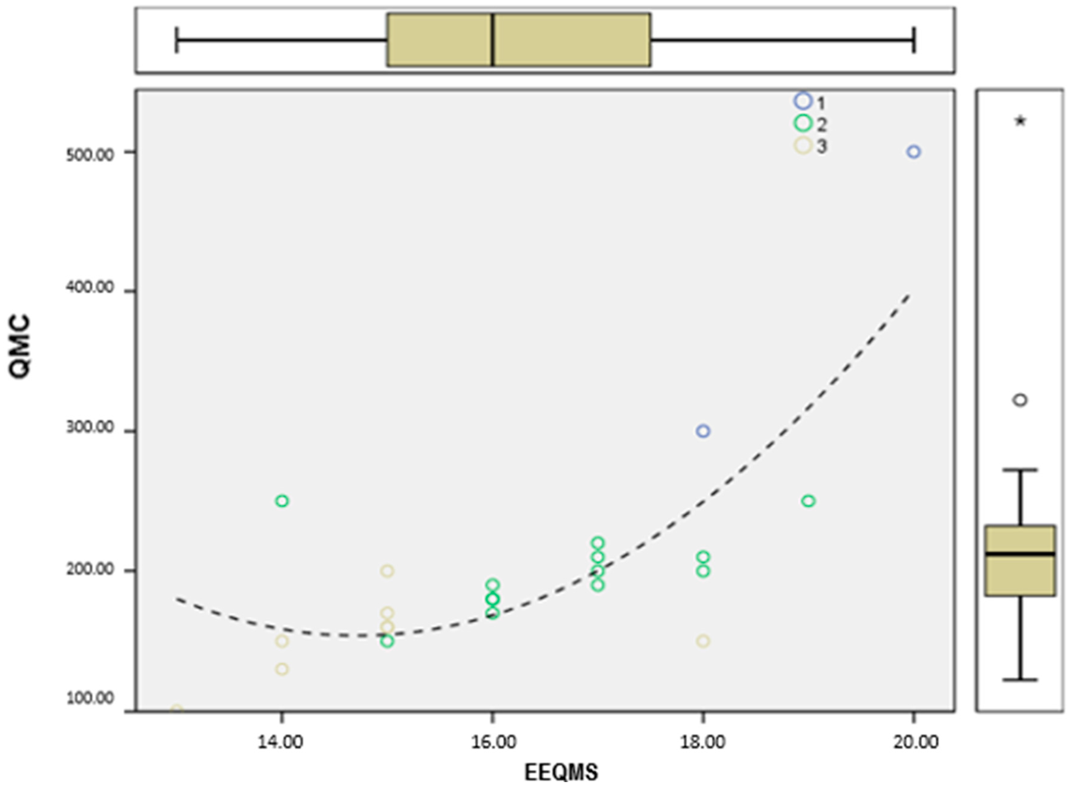
The Figure 8 illustrates the relationship between the economic efficiency of quality management systems (EEQMS) and quality management costs (QMCs) for companies grouped into three clusters. The clusters are represented by different colors: blue for Cluster 1, green for Cluster 2, yellow for Cluster 3. The figure demonstrates that as the economic efficiency of the QMS increases, the quality management costs also rise, which is confirmed by the dotted trend curve. More economically efficient companies tend to invest more in quality management.

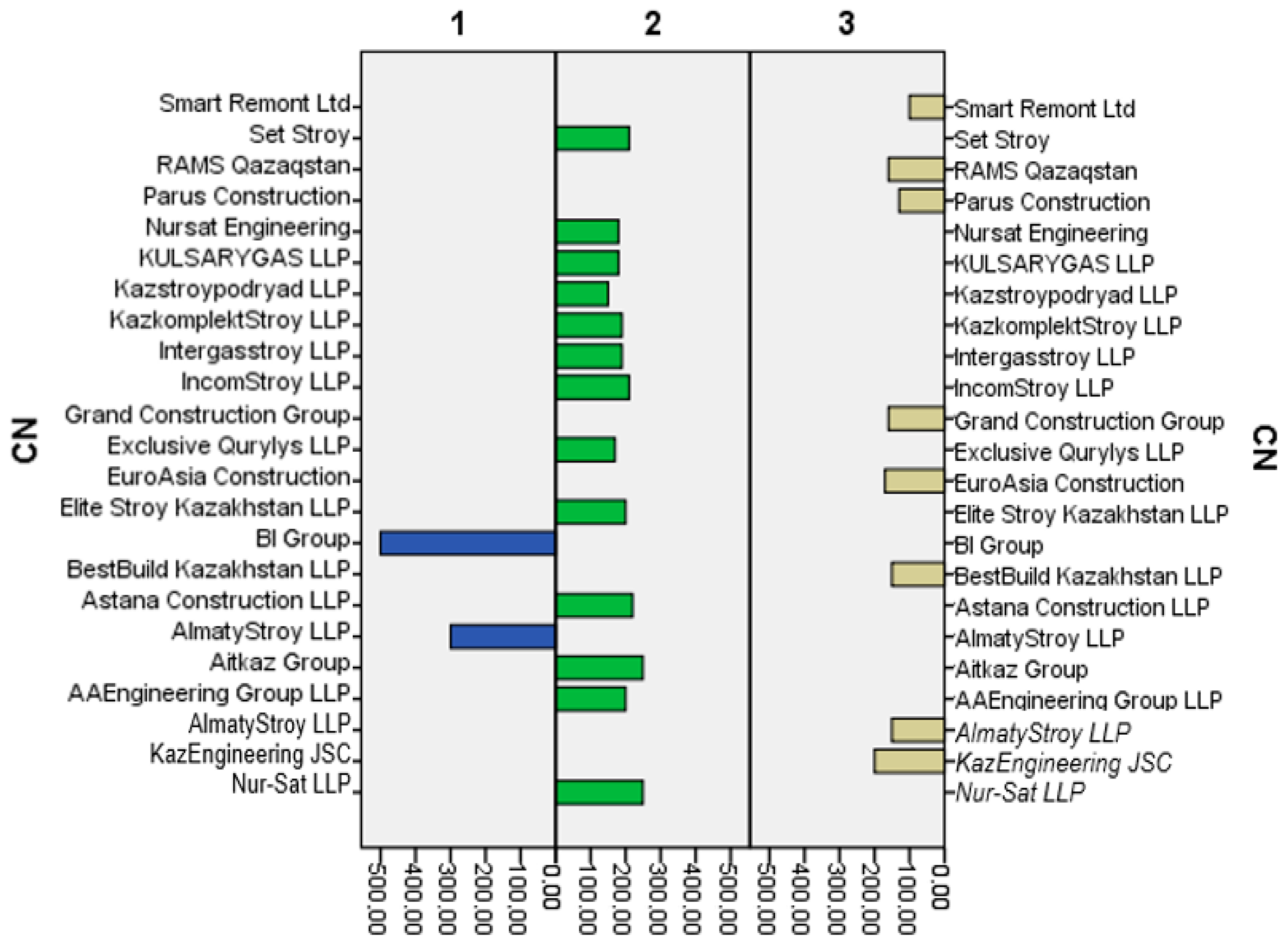
The Figure 9 illustrates the distribution of quality management costs (QMCs) among construction companies grouped into three clusters. Clusters 1, 2, and 3 are represented by differently colored columns. The table shows that companies in Cluster 1 (BI Group and AlmatyStroy LLP) have significantly higher quality management costs compared to other clusters. In Cluster 2, average QMCs are moderate, with companies such as Kazstroypodryad LLP and Elite Stroy Kazakhstan LLP demonstrating diversity in cost levels. Cluster 3 is characterized by lower QMC values, as seen in companies like Smart Remont Ltd. and Set Stroy.

Companies in Cluster 1 invest more in quality management, which may be linked to their leading positions in the market. Cluster 2 companies exhibit balanced quality costs, while Cluster 3 companies have low QMCs, suggesting a need for optimization in their quality management processes.

The cluster analysis of construction companies reveals significant differences in key indicators of quality management costs (QMCs), economic efficiency (EEQMS), customer satisfaction level (CSL), and the company’s period of operation (PO). Companies in Cluster 1, such as BI Group and AlmatyStroy LLP, are characterized by the highest quality management costs and high indicators of cost effectiveness and customer satisfaction. Large companies, which actively invest in quality, are more likely to achieve leading market positions. Companies in Cluster 2 display stable indicators, suggesting growth opportunities through more effective quality management.

Companies in Cluster 3 have the lowest values across all indicators, especially for quality management costs, which may indicate less developed management processes. Firms such as Smart Remont Ltd. and Set Stroy could face challenges in improving their competitiveness in the market without additional investments in products and services quality.

The results of the analysis emphasize the importance of systematic quality management for improving economic efficiency and customer satisfaction. It is recommended that companies in the second and third clusters review their quality management strategies to enhance efficiency and strengthen their market positions.

The results of this study indicate that quality management is a key factor in improving cost efficiency and customer satisfaction in construction companies.

The results of the regression analysis revealed a significant relationship between quality management costs (QMCs) and profitability indicators, which confirms the importance of investments in quality to achieve high financial results.

The cluster analysis divided companies into three groups based on their quality management cost and performance, highlighting differences in management strategies. Companies in Cluster 1, which actively invest in quality management systems, demonstrate leading positions in profitability and customer satisfaction. In contrast, companies in Clusters 2 and 3 allocate less funding for quality management and, consequently, achieve lower results.

Comparative Analysis with Prior Research. The findings of this study are consistent with several prior works. For example, Gonzalez and Rodriguez identified a positive relationship between customer-oriented QMS implementation and customer satisfaction, which is also evident in our results. Similar associations were reported by Chen and Li and Psomas and Jaca, who emphasized the role of QMSs in improving process efficiency and maintaining consistent quality. Our findings also align with Kaynak, who argued that the integration of QMS practices contributes to enhanced operational performance through standardization and process control.

However, some discrepancies were observed. Unlike Talib et al. [9], who reported a stronger impact of QMSs on financial outcomes, our results indicate a more moderate effect. This may be explained by the specific structure of the construction sector in Kazakhstan and differences in the maturity level of quality management practices across companies. Furthermore, many international studies are based on larger sample sizes and utilize more sophisticated tools to measure customer satisfaction, which may account for the variation in findings.

Overall, while our study supports the general trends observed in previous research, it also introduces context-specific insights that deepen the understanding of QMS implementation in Kazakhstan’s construction industry.

5. Conclusions

This study confirms that the implementation of customer-oriented quality management systems (QMSs) has a significant positive impact on the performance of construction companies in Kazakhstan. The analysis identified three distinct clusters of companies based on QMS investment, operational experience, and performance outcomes.

Cluster 1 companies, demonstrating high efficiency and customer satisfaction, serve as benchmarks. These firms should continue advancing QMS practices through digital platforms, real-time feedback tools, and enhanced certifications.

Cluster 2 firms, with moderate performance, are advised to strategically optimize QMS-related expenditures—focusing resources on areas such as customer feedback, staff training, and complaint resolution. Policymakers could support this group through targeted incentives and subsidized training programs.

Cluster 3 companies show low investment in QMSs and underperform in profitability and satisfaction. For them, implementing baseline systems like ISO 9001 and strengthening internal audits and documentation practices is critical. Support from industry associations in the form of technical tools and benchmarking resources can aid their development.

At the policy level, there is a clear need for regulatory frameworks that promote QMS adoption, particularly among SMEs. QMS certification could be required in public procurement, and integration of QMS topics into vocational and higher education curricula would help build long-term capacity.

For sustained quality improvement, companies should adopt continuous improvement models, conduct regular evaluations, and foster a culture of transparency and customer orientation. These strategies are vital for maintaining competitiveness in a dynamic construction market.

This study demonstrates the link between QMSs and broader sustainability goals. An effective QMS reduces waste, improves resource efficiency, and strengthens environmental performance. It also reinforces corporate social responsibility, positioning QMSs as strategic drivers of sustainable construction.