Freight Mode Choice with Emission Caps: Revisiting Classical Inventory and Transportation Decisions

Abstract

Freight mode choice and the resulting inventory implications significantly influence a product’s carbon footprint. This paper investigates mode selection under a voluntary carbon emissions constraint. Slower modes such as inland waterways and ocean freight are less expensive and emit less greenhouse gas (GHG), but they require higher inventory levels due to longer lead times. In contrast, faster modes like less-than-truckload (LTL) shipping reduce inventory needs but incur higher transportation costs and emissions. Mode choice thus involves trade-offs between transport cost, inventory holding, lead time uncertainty, and GHG emissions from transportation and warehousing. This paper develops a comprehensive inventory-transportation model under the stochastic demand and lead time to evaluate these trade-offs and guide sustainable freight decisions. The model is a practical toolbox that enables managers to evaluate how freight mode choice and inventory policy affect costs and emissions under different operational scenarios and carbon constraints.

1. Introduction

The sixth assessment of the Intergovernmental Panel on Climate Change (IPCC) reported the following [1]:

“Human activities, principally through emissions of greenhouse gases, have unequivocally caused global warming, with global surface temperature reaching 1.1 °C above 1850–1900 in 2011–2020.”

Since the 1750s, atmospheric carbon dioxide concentrations have risen from approximately 280 to over 400 parts per million (ppm), driven largely by the burning of fossil fuels for energy, transportation, and industrial activities. Global supply chains—through their reliance on freight transport and warehousing—have emerged as a growing contributor to these emissions. To mitigate the effects of global warming, the IPCC estimates that emissions will need to be reduced by 50% by 2050 and by 80% by 2080.

As firms increasingly commit to decarbonizing their supply chains, common logistics decisions—such as freight mode selection and inventory policy decisions—have become important levers for carbon mitigation. This paper focuses on choosing the appropriate freight mode (truck, rail, intermodal, etc.) and its impact on emissions, particularly when combined with inventory decisions.

Freight activity in the United States is projected to increase from 5.2 trillion ton-miles in 2020 to over 8.1 trillion by 2050 [2], with trucking continuing to dominate domestic goods movement [3]. Freight accounts for an estimated 27–32% of transportation-related GHG emissions [4,5]. Estimates for the emissions from warehouses range from 11 to 30% [6,7,8]. These emissions are driven by growing shipment volumes, globalization of supply chains that warrant higher inventory, and increased reliance on carbon-intensive modes of transportation, such as truck fleets versus rail (see, for example, [9]). The increasing rate of freight-related emissions has prompted policy initiatives aimed at decarbonizing freight operations [10,11].

In the absence of binding regulations, especially in the United States, many firms mitigate emissions to meet stakeholder expectations and prepare for future climate policy. Understanding how carbon constraints affect operational trade-offs is critical to designing cost-effective, low-emission supply chains.

This paper adds to the growing research stream on carbon mitigation by providing a model for freight choice with voluntary carbon emission constraints. Our contributions are in three areas. First, our model uses a continuous-review reorder-point stochastic inventory control context to compute the optimal lot size, reorder point, and mode choice for a given product and freight mode characteristics. Second, the model uses a comprehensive inventory-transportation cost framework, encompassing the cost of ordering, holding cycle, safety, in-transit inventory, and cost of transportation. Third, we use emissions from transportation and warehousing as a voluntary constraint; these emission levels are motivated by well-established protocols such as the GHG protocol.

The paper is organized as follows. Section 2 reviews the relevant literature. Section 3 introduces the notation and develops the cost model. Section 4 gives a numerical illustration (with managerial insights) based on our experience with a common carrier. In Section 5, we present our conclusions and directions for future research.

2. Review of the Relevant Literature

The freight choice problem—or the trade-off between inventory and transportation—has a long history in the logistics and supply chain literature (see [12,13] and the references within for a comprehensive review). Much of the research has focused on the mode choice decision from an inventory-logistic perspective, studying the impact of various logistics parameters (such as demand, lead time, product characteristics, and origin-destination dynamics) on the decision. Shipments via faster and reliable modes (such as airfreight or truck) can track customer demand and necessitate less inventory, but they are expensive, while slower modes of transport (rail or ocean container shipping) are cheaper, but they have longer lead times, requiring higher cycle, safety, and in-transit inventories. Studies have often used a total logistics cost perspective to evaluate such trade-offs. Furthermore, the conventional wisdom is that firms shift to slower and higher capacity modes as freight volumes grow.

Research streams on sustainability, specifically those related to supply chains, have grown significantly in the last two decades (early examples include [14,15,16,17,18,19]). Much of the research has focused on strategies and concepts to run sustainable supply chains, including product design, designing low-energy processes, reducing waste, and establishing reverse logistics and closed-loop supply chains [20,21]. Recent developments reflect growing regulatory pressures, such as the European Union’s Carbon Border Adjustment Mechanism (CBAM) and expanded cap-and-trade programs, pushing firms to incorporate emissions reduction targets into core supply chain decisions [22].

There is also a growing body of research on integrating carbon constraints into inventory-logistics theoretical frameworks (see, for example, [23]). Models include emissions as a constraint or a cost within a cap-and-trade system. Benjaafar et al. [24] demonstrated that firms can adjust their operations to meet emissions targets with minimal cost penalties. Hua et al. ([25]) and Chen et al. [26] extended the EOQ model to incorporate carbon trading.

Research streams also explicitly addressed freight mode selection under carbon considerations. Hoen et al. [27] provided a stochastic inventory model that incorporates the carbon emission cost per unit as part of the cost function and a constraint. They found the mode and the “order-up-to” inventory policy that minimized cost. They concluded that emission costs do not significantly impact mode choice. However, a cap on emissions may necessitate an increase in cost. In a related paper, Hoen et al. [28] extended the model to multiple products, where the demand is a function of the price. The model determines the optimal price and the mode that maximizes profit. Both of these papers used the NTM [29] to compute emissions and restrict their emissions analysis only to freight. Arikan et al. [30] considered a scenario where two sources of resupply—air and ocean containers—were available and used simulations to study economic and emission performance within an inventory-logistic framework. They used both freight and warehouse emissions to compute the total GHG emissions. Their primary focus was to study the effect of variability on performance.

Recent studies further refined these findings by incorporating dynamic decision-making frameworks. Eksioglu et al. [31] developed optimization models incorporating multiple transportation modes, showing how carbon regulatory mechanisms influence supply chain decisions by balancing transportation costs, inventory holding costs, and emissions. Chang et al. [32] proposed a multimodal transport path optimization model under low-carbon policies, considering uncertain cargo demand and transportation costs while integrating carbon emissions as constraints. AI-driven freight optimization, digital twin technologies, and real-time emissions tracking now enable firms to make dynamic mode selection decisions based on both economic and environmental considerations [33,34]. As part of their sustainability commitments, companies across industries have initiated pilot programs for alternative fuel vehicles, such as BMW’s deployment of hydrogen-powered trucks in Europe [35] and BNSF Railway’s collaboration with Caterpillar and Chevron to develop a hydrogen-powered locomotive [36].

Our paper adds to the literature by exploring the economic and environmental performance of mode choice decisions within the context of a $(Q,r)$ inventory policy. This is common when a resupply is performed in predetermined lot sizes (pallets, containers, etc.). The policy is set in a stochastic environment that can accommodate various forms of lead time demand distributions. Second, our emission computations include a broader framework that includes both freight and warehousing, reflecting that slower, less carbon-intensive freight movement may, in fact, negatively impact emissions due to larger inventory stockpiles. Finally, our model is flexible enough to accommodate a wider variety of mode characteristics—lead-time, cost, and emission efficiency—into a comprehensive inventory-logistics cost framework, encompassing ordering, holding, inventory, and transportation costs.

3. Model Development

• Notation

Decision Variables:

• Q = order size from the supplier. This will also determine the freight mode that is used.
• r = reorder quantity.
• m = index representing the mode. Typical mode choices include less-than-truckload (LTL), truckload (TL), intermodal (TOFC), carloads (Rail), and air freight.

Cost Function

• $ETAC(Q,r,m)$ = expected total annual costs given Q, r, and m.

Variables and Constants

• $\lambda$ = yearly demand.
• d = number of days in a year.
• u = daily demand, a random variable with a mean ${\mu }_d$ and standard deviation ${\sigma }_d$.
• $L_m$ = lead time for the mode m, a random variable with a mean ${\mu }_m$ and standard deviation ${\sigma }_m$.
• $D_{ltd}$ = lead time demand, a random variable with a mean ${\mu }_{ltd}$ and standard deviation ${\sigma }_{ltd}$.
• w = weight of the product.
• S = ordering cost.
• h = inventory cost per unit of inventory per year.
• $\rho$ = desired service level.
• $\eta \left(r\right)$ = backorders per replenishment cycle.
• $\pi$ = cost of backordering one unit.
• D = distance the freight is moved.
• $T{C}_m(Q,D)$ = transportation cost for a given mode m moving a lot size Q a distance D.
• M = freight movement expressed in weight-distance. If Q units are moved a distance D, then $M=QwD$.
• $f_{m,T}$ = efficiency of freight mode m expressed in weight-distance per unit of fuel.
• $e_T$ = emission factor of a unit of fuel.
• $e_I$ = emission factor per unit of product held in inventory.
• $C_B$ = the carbon emission budget for the year.

• Model Context and Assumptions

The context of our model is a firm that distributes a product from stock. It faces uncertain demand downstream in the supply chain; the daily demand u is a random variable. The annual demand is $\lambda$ units. The firm continuously monitors the inventory levels at the warehouse and, based on a chosen service level $\rho$, orders Q units from the supplier when the inventory level falls below a critical level r. The firm also decides on the choice of freight (m) (i.e., how the order will be shipped). The freight mode m has an uncertain lead time $L_m$, which is assumed to be a random variable. The firm also tracks its emissions related to freight and warehousing operations. While carrier operations may technically not be part of firm operations, it is included in the so-called “Scope 3” emissions [20], which takes a more supply chain-centric approach when computing emissions. The firm has voluntarily imposed a constraint on GHG emissions from freight and warehousing emissions at a level $C_B$.

The objective is to find the optimal levels of $Q,r,$ and m that minimize the total cost of ordering, holding inventory, and transportation. The solution must satisfy service and emission constraints, as well as restrictions on mode capacity.

Slower transport modes like inland waterways and ocean freight are cheaper and likely have lower transport-related GHG emissions but also necessitate higher cycle, safety, and in-transit stocks, making inventory costs and the corresponding carbon emissions from inventory higher. On the other hand, faster modes like LTL shipping are quick and warrant lower stock (and lower warehouse-related emissions) but are expensive and, on average, have higher GHG emission levels during transport. Deciding on the appropriate mode to use is a trade-off between the uncertainty of demand and lead time, the cost to transport, and the GHG emission levels of transportation and warehousing.

• Model

The key objective of the model is to find $Q,r,$ and m to minimize the expected total annual cost $ETAC$:

$$\begin{array}{ccc}\hfill ETAC(Q,r,m)& =& \lambda /Q\ast S+[Q/2+(r-{\mu }_{ltd})+\lambda \ast {\mu }_m/d]h\hfill \\ & +& \eta \left(r\right)\ast \lambda /Q\ast \pi \hfill \\ & +& T{C}_m(Q,D)\lambda /Q\hfill \end{array}$$

(1)

subject to

$$\begin{array}{c}\hfill \eta \left(r\right)\le Q(1-\rho )\end{array}$$

(2)

$$\begin{array}{c}\hfill M/f_{m,T}{e}_T\ast \lambda /Q+[Q/2+(r-{\mu }_{ltd})]e_I\le C_B\end{array}$$

(3)

$$\begin{array}{c}\hfill Q\le Q_m\end{array}$$

(4)

$$\begin{array}{c}\hfill Q,r\ge 0\end{array}$$

(5)

The first term in Equation (1) is the ordering cost. If Q units are ordered, then there are $\lambda /Q$ replenishment cycles in a year, and thus the total cost is $\lambda /Q\ast S$. The second term of the cost function is the inventory holding costs. It consists of three components. The first is the cycle inventory, which is denoted by $Q/2$. The second component is the safety stock, or the stock held in excess of the mean lead time demand ${\mu }_{ltd}$ to meet a given service level $\rho$. The third component is the in-transit inventory, or the average stock in transit over the course of the year. Since the total demand is $\lambda$ with d days in a year, ${\mu }_m/d$ is the average lead time in years. The in-transit inventory is simply $\lambda \ast {\mu }_m/d$. The three components are multiplied by h, the cost of holding a unit for a year. The third term in the cost function is the total backorder cost, while $\eta \left(r\right)$ is the total number of backorders per replenishment cycle, with each unit backordered costing $\pi$. The fourth term is the cost of transportation for a given distance and lot size.

• The Constraints

Equation (2) is the service level constraint. If $\rho$ is the desired level of service, then the planned shortage per replenishment cycle (ESPRC) is $Q(1-\rho )$. For a given r, the expected shortage is $\eta \left(r\right)$. Equation (3) is the constraint on the total carbon emissions per year. As the ensuing section will show, the total emissions are the sum of the emissions from transportation, given a type of fuel, and the emissions incurred when the product is held in inventory. $C_B$ is the planned or budgeted level of emissions. Equation (4) is the constraint on the freight mode capacity, and Equation (5) is the non-negativity constraints on Q and r.

3.1. Computing $\eta \left(r\right)$

For a given reorder point r, a freight mode m, and lead time demand $D_{ltd}$, we have

$$\eta \left(r\right)={\int }_r^{\infty }(x-r)D_{ltd}\left(x\right)dx$$

(6)

Managers often estimate $D_{ltd}$ from empirical data by observing demand over multiple replenishment periods. Statistically, if the mean and standard deviation of both the daily demand (${\mu }_d,{\sigma }_d$) and lead time (${\mu }_m,{\sigma }_m$) are known, then the mean and standard deviation of the lead time demand can be calculated as ${\mu }_{ltd}={\mu }_d{\mu }_m$ and ${\sigma }_{ltd}=\sqrt{{\mu }_d^2{\sigma }_m^2+{\mu }_m{\sigma }_d^2}$, respectively. The shape of the lead time demand is typically assumed to be normal for fast-moving consumer goods [37]. The gamma distribution is often used for medium to slow-moving goods or when lead times have a long tail [38]. This is often true when using slower modes of transport, as chances that shipments are delayed during transit are higher and therefore can result in lead time demand distributions with longer tails The Poisson distribution is often used for slow-moving items.

Table 1. Calculating $\eta \left(r\right)$ for different stochastic environments.

Demand	Normal	Gamma	Poisson
pdf	$g\left(x\right)={\displaystyle \frac{1}{\sigma \sqrt{2\pi }}}{e}^{{\displaystyle \frac{-{(x-\mu )}^2}{2{\sigma }^2}}}$	$\gamma (\alpha ,\beta )={\displaystyle \frac{x^{\alpha -1}{e}^{-x/\beta }}{{\beta }^{\alpha -1}\Gamma \left(\alpha \right)}}$, $\alpha ,\beta \ge 0$	$P(x=k)=e^{\delta x}{\left(\delta x\right)}^k/k!,x\ge 0$
Mean	$\mu$	$\alpha \beta$	$\delta$
Standard Deviation	$\sigma$	$\alpha {\beta }^2$	$\delta$
$\eta \left(r\right)$	$\left[f\right(z)-z(1-F\left(z\right)\left)\right]\sigma$	$\alpha \beta (1-G_1\left(r\right)-r(1-G_2\left(r\right))$	$\delta (1-E_1(r-1)-r(1-E_1\left(r\right))$
Notes	$f(.)$ and $F(.)$ are the pdf and cdf of the standard normal distribution, where $z=(r-\mu )/\sigma$	$G_1(.)$ and $G_2(.)$ are the cdfs of $\gamma (\alpha ,\beta )$ and $\gamma (\alpha +1,\beta )$, respectively	$E_1(.)$ is the cmf of $P(.)$

shows how $\eta \left(r\right)$ can be computed for different stochastic environments. The lead time demand ($D_{ltd}$) can take any of the three forms, and the corresponding characteristics of the pdf and computational formulas for $\eta \left(r\right)$ are available in the table below [39,40].

3.2. Calculating Carbon Emissions

For the purposes of this paper, the total emissions are the sum of the emissions from the burning of fuel by the vehicles used for transporting freight and the emissions from warehousing activities. Emissions are typically reported as carbon dioxide equivalents (CO₂e) in weight units (lbs, kgs, etc.). While there is no universal standard to calculate emissions, most are based on the Greenhouse Gas (GHG) Protocol. The GHG Protocol is a common approach to emissions reporting developed by the World Resources Institute (WRI) and the World Business Council for Sustainable Development (WBCSD).

3.2.1. Emission of Freight

The most direct method to calculate emissions from freight transport is to measure the fuel consumed and multiply it by the emission factor for that particular kind of fuel. If direct fuel usage is unavailable, then indirect approaches are used to estimate fuel use. These include estimating fuel use from fuel cost (by using the average cost of a unit of fuel) or from statistics that most freight operators log—distance and load carried—and then using them in combination with efficiency measures that estimate fuel use from these data. In this paper, we assume that the shipper logs distance and load data, and we estimate fuel use using efficiency measures. (If fuel usage is available, then this step can be bypassed). Once fuel use is known, the emissions can be computed using the appropriate emission factor. Fuel efficiency measures can vary significantly depending on the product being hauled, the equipment hauling it, the geographical location, and the load (percent empty and back hauls). In our experience, firms use averages, by mode, of the overall shipments made in preceding months or years.

Table 2. Efficiency and emission factors for common freight modes.

Efficiency		Emission Factors
Freight Mode	Ton-Miles/Gallon Range	Fuel	Kg CO2/Gallon
Rail		Diesel Fuel	10.19
Double-Stack	226–512	Kerosene/Jet Fuel	9.88
TOFC/Box Car	406–469	Aviation Gasoline	8.31
		Propane	5.75
Truck		Motor Gasoline	8.49
Dry Van	82–110
Flatbed	112–133
Container	68–100
Barge	576
Ocean Container	575–1043

gives the average efficiency measures for common freight mode types and emission factors for standard fuels [41].

It is common among shippers to report freight movement in weight-distance measures (for example, ton-mile). If D is the distance, w is the product’s weight, and the chosen lot size is Q, then the movement ($M=QwD$) is the weight-distance statistic per replenishment cycle. Meanwhile, $f_{m,T}$ is the efficiency of the mode m, given the type of fuel T used. This is usually expressed in terms of weight-distance per unit of fuel (for example, ton-mile/gallon). $M/f_{m,T}$ computes the total fuel usage per replenishment cycle. Therefore, the fuel consumption per replenishment cycle is $M/f_{m,T}\ast e_T$, where $e_T$ is the emission factor of a unit of fuel. Since there are $\lambda /Q$ cycles, the yearly emissions related to freight movement are $M/f_{m,T}\ast e_T\ast \lambda /Q$.

3.2.2. Carbon Emissions of Inventory

The inventory that is delivered from the supplier is assumed to be warehoused. We assume this warehouse can accommodate inventory from any of the freight modes under consideration. We also assume that the emissions related to the inventory are proportional to the energy use—direct or indirect—to maintain the warehouse. This would include electricity, climate control, and moving operations such as forklifts within the warehouse. We have assessed an emission factor per unit of inventory; as the inventory increases, energy related to maintenance and servicing also rises proportionally. For typical packaged goods stocked in and fulfilled from warehouses, the emissions resulting from transportation operations far outweigh the emissions from warehousing, and unless significant energy is expended on warehousing (for example, a large proportion of freezers and special handling circumstances), this component typically has a smaller impact on the mode choice.

The choice of Q and r determines the average inventory in the warehouse. An emission factor $e_I$ is applied to each unit of cycle inventory ($Q/2$) and the safety stock $(r-{\mu }_{ltd})$ to compute the emissions related to inventory, where $[Q/2+(r-{\mu }_{ltd})]e_I$.

3.3. Transport Cost

Freight costs are a function of the mode, product class, distance, weight, and volume. In this paper, we model transportation as a function of the lot size Q, the weight w, and the distance d. For the less-than-truckload mode, the rates per unit weight of the product decrease as the total weight that is shipped increases. We model the rate R (in $/cwt) as $R=m+nln\left(Qw\right)$ [42], where m and n are constants. The cost of LTL shipments is R (in $/cwt)*$Qw$(in cwt). The rates are typically quoted as full loads (rates to ship $Q_m$) between the origin and destination for truckload, carload, and containerized freight. Intermodal rates are tailored and usually a function of the weight, the equipment used (TOFC or double stack, etc.), and the origin and destination. Our model can handle any freight cost scheme as long as it depends on the weight and distance traveled.

3.4. Solution Procedure

Equation (1) is discontinuous in m since each mode has its cost structure, freight parameters, and carbon emissions. For a given m, however, Equation (1) is continuous but nonlinear in Q and r. Equation (1) can be solved using the generalized reduced gradient (GRG) algorithm (see [43]). We implemented the GRG optimization algorithm using Frontline Systems Inc.’s Analytic Solver Platform [44]. The typical procedure is to fix m and compute the optimal Q, r, and $ETAC$ for each m that satisfies the service, capacity, and carbon constraints (this would be the classic inventory-theoretic problem with added carbon constraints). The mode m that gives the lowest cost would then be chosen. Since, at any given level of $\lambda$, only a subset of modes is usually considered, (For example, for small volumes, the choices are typically LTL, TL, or intermodal. As volumes grow, the choices shift toward modes with larger capacities, like rail and waterways.) the solution procedure is often computationally less intensive than an entire grid search over all available transport modes.

4. Numerical Illustration and Discussion

4.1. Illustration

To illustrate our model, we considered product and freight characteristics that were representative of the consumer packaged goods (CPG) industry. CPG products are everyday items such as food, beverages, personal care products, and household cleaning supplies, which are consumed quickly and require frequent replenishment. These products are relatively low in cost, have high turnover rates, and are distributed through extensive retail networks. Our product was assumed to have a unit cost of USD 30 and a weight of 2 lbs, with an annual demand of 100,000 units (see [45] for typical product prices and [37] for comparable examples in multiple categories). Daily demand was uncertain, with a mean ${\mu }_d=\lambda /d$ of 273.97 units and a standard deviation ${\sigma }_d$ of 50 units. Other input parameters relevant to the model are given in

Table 3. Input parameters.

Product Characteristics
Expected annual demand	$\lambda$	100,000	per year
Number of days in a year	d	365
Mean demand per day	${\mu }_d$	273.97	items
Std dev. of demand per day	${\sigma }_d$	50	items
Cost per item	C	$30	per item
Weight per item	w	2	lb. per item
Emissions from inventory	$e_I$	0.01	per item
Cost of placing an order	S	$500	per order
Inventory carrying charge	h	$0.15	per USD per year
Backorder cost	$\pi$	$10	per unit
Service level	$\rho$	95%
Carbon cap	$C_B$	10,000	KgCO2 per year
Mode Characteristics
Name (m)	LTL	TL	TOFC	Carload
Rate ($T{C}_m(Q,D)$, per shipment)	$67-6ln\left(Q\right)\ast Qw$	USD 3031	USD 2500	USD 1750
Mean lead time (${\mu }_m$, days)	6	3	7	10
Distance (D, in miles)	500	500	500	500
Standard deviation (${\sigma }_m$,days)	0.6	0.3	0.7	1
Capacity ($Q_m$, lbs)	40,000	40,000	40,000	90,000
Fuel efficiency ($f_{m,T}$, ton-mile/gallon)	100	100	400	500

.

The supplier was at a 500-mile distance, and four choices for the freight mode were available: less-than-truckload (LTL), truckload (TL), the intermodal option of trailer-on-flat-car (TOFC), and rail carloads. The fuel efficiency of these modes is comparable to the estimates in Table 2. Table 3 also gives the mode choices’ rates, lead time characteristics, capacities, and fuel efficiency ratings. In this example, the LTL rates were quoted per cwt and given by $67-6ln\left(Qw\right)$. Thus, as the weight shipped increased, the rate decreased. This was multiplied by the weight $Qw$ in cwt to compute the cost of shipping each replenishment cycle. For TL, TOFC, and carloads, the shipper had a quoted per shipment rate. (Irrespective of how much was shipped, a constant rate was charged.) The model is flexible, but to incorporate a tiered shipping rate (if shippers offer the option), then for ease of exposition, we assumed that the firm would use the entire capacity of the mode when used. We also chose for the lead time demand distribution to be a gamma random variable (see also [37]).

In addition to transportation costs, the model accounts for greenhouse gas (GHG) emissions from both transportation and warehousing. The firm operates under a voluntary carbon cap of 10,000 kg CO₂ per year, with transportation emissions calculated using fuel efficiency (in ton-miles per gallon) and an emissions factor of 10.19 kg CO₂ per gallon of diesel. Warehousing each unit accounts for 0.01 Kg CO₂.

These freight modes differ not only in cost and emissions but also in operational characteristics that impact inventory. LTL and TL have similar fuel efficiencies and emissions, but TL shipments are faster and benefit from flat-rate pricing due to full truckload utilization. TOFC shares TL’s capacity but is slower, and its higher fuel efficiency results in lower transportation emissions. Carload has the highest capacity and lowest per-shipment cost but also the longest lead time. This increases inventory exposure, particularly under higher values of inventory carbon intensity ($e_I$). While LTL and TL are frequently used for CPG products due to their responsiveness, rail-based modes like TOFC and carload offer compelling trade-offs for cost and emissions that depend on the product’s storage characteristics, demand variability, and service level requirements. The model accommodates these complexities and provides a platform to evaluate how mode choice interacts with inventory dynamics under varying cost, risk, and sustainability constraints.

Table 4. Model results.

Derived Elements
Expected demand during lead time	${\mu }_{ltd}$	1643.83	units
Expected backorders	$\eta \left(r\right)$	3.57	per replenishment cycle
Total number of trips	$\lambda /Q$	12.15	per year
Ship weight	$Qw$	16,455.06	lbs per replenishment cycle
Cost of shipping	$T{C}_m(Q,D)$	$2124.11	per replenishment cycle
Average inventory	$Q/2+r$	6141.83	in warehouse + in transit
Decisions
Reorder point	r	2028.06	units
Order quantity	Q	8227.53	units
Mode	m	LTL
Costs
Ordering	$S\lambda /Q$	$6077.15	per year
Inventory carrying	$(Q/2+r)h$	$20,240.99	per year
Backorder costs	$\eta \left(r\right)\pi \lambda /Q$	$434.80	per year
Transport costs	$T{C}_m(Q,D)\lambda /Q$	$25,817.10	per year
Expected total annual cost	$ETAC(Q,r,m)$	$52,570.05	per year
Carbon Computations
Transportation	$M/f_{m,T}{e}_T\ast \lambda /Q$	5105	CO2 kg per year
Inventory	$Q/2+(r-{\mu }_{ltd})e_I$	61.41	CO2 kg per year
Total		5166.41	CO2 kg per year
Budget	$C_B$	10,000	CO2 kg per year

gives the results of the model. In this case, LTL is the mode that minimized costs, given the constraints on service (95% availability), mode capacity (40,000 lbs), and GHG emissions (capped at 10,000 Kg of CO₂). The firm optimally would order 8227.53 units (to be shipped by LTL) when the inventory reached below 2028.06 units. The transport costs were significant (almost 50% of total costs), and 98.8% of the emissions were from transportation.

4.2. Sensitivity Analysis

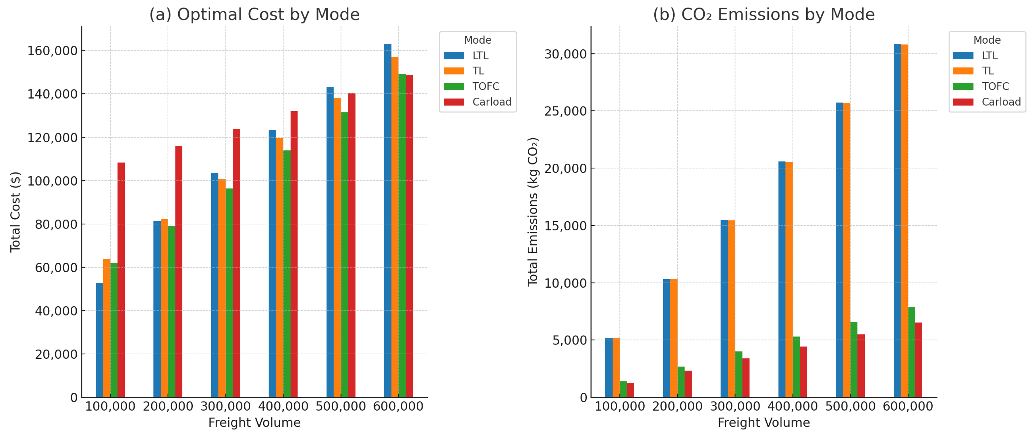
Figure 1a,b illustrates the sensitivity of the transportation cost and emissions to changes in freight volume. At lower volumes, when $\lambda$ = 100,000, LTL emerged as the option with the lowest cost and fell well below the standard carbon cap of 10,000 kg CO₂. However, as the volume increased, the cost structure shifted in favor of TOFC when 20,000 $\le \lambda \le$ 500,000 and eventually carloads at higher volumes, reflecting the economies of scale in the bulk freight modes. Emissions also rose with the volume but not uniformly across all modes. LTL and TL exhibited steep increases in CO₂ emissions, while TOFC and carloads remained substantially lower, making them more attractive even from an environmental standpoint at higher scales of operation.

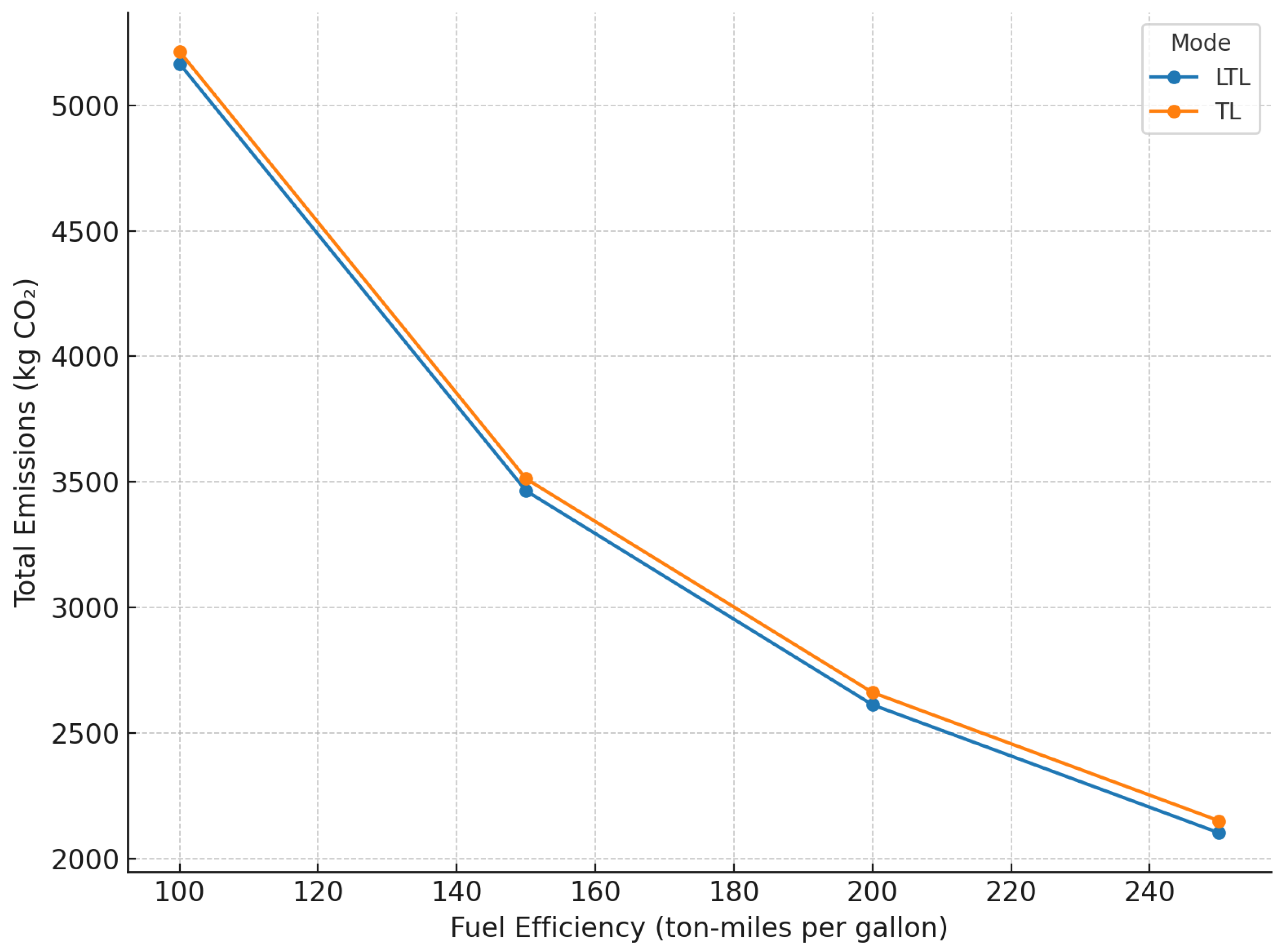
Figure 2 extends the analysis by illustrating how the total emissions from LTL and TL responded to improvements in fuel efficiency, measured in ton-miles per gallon. As the efficiency increased, emissions declined sharply, suggesting that compliance with carbon constraints need not rely solely on switching to lower-emission modes like TOFC or carloads. At a volume of 100,000 units, LTL emitted 5166 kg CO₂ at 100 ton-miles per gallon. If the carbon cap were tightened to 5000 kg CO₂, this would disqualify LTL in its current form and shift the optimal mode to TOFC—despite its higher cost—illustrating how policy constraints can directly influence mode selection. However, by improving fuel efficiency to 150 ton-miles per gallon, LTL’s emissions fell to 3465 kg CO₂, bringing it back under the cap. When $\lambda$ = 100,000, TOFC was USD 9422 more expensive than LTL. If emissions-reducing upgrades (such as aerodynamic kits, hybrid powertrains, or optimized routing) cost less than this premium, then the firm can preserve LTL’s flexibility while remaining compliant. This gives managers a meaningful trade-off; rather than defaulting to a more expensive mode, they can evaluate the cost-effectiveness of improving their current operations to meet sustainability goals.

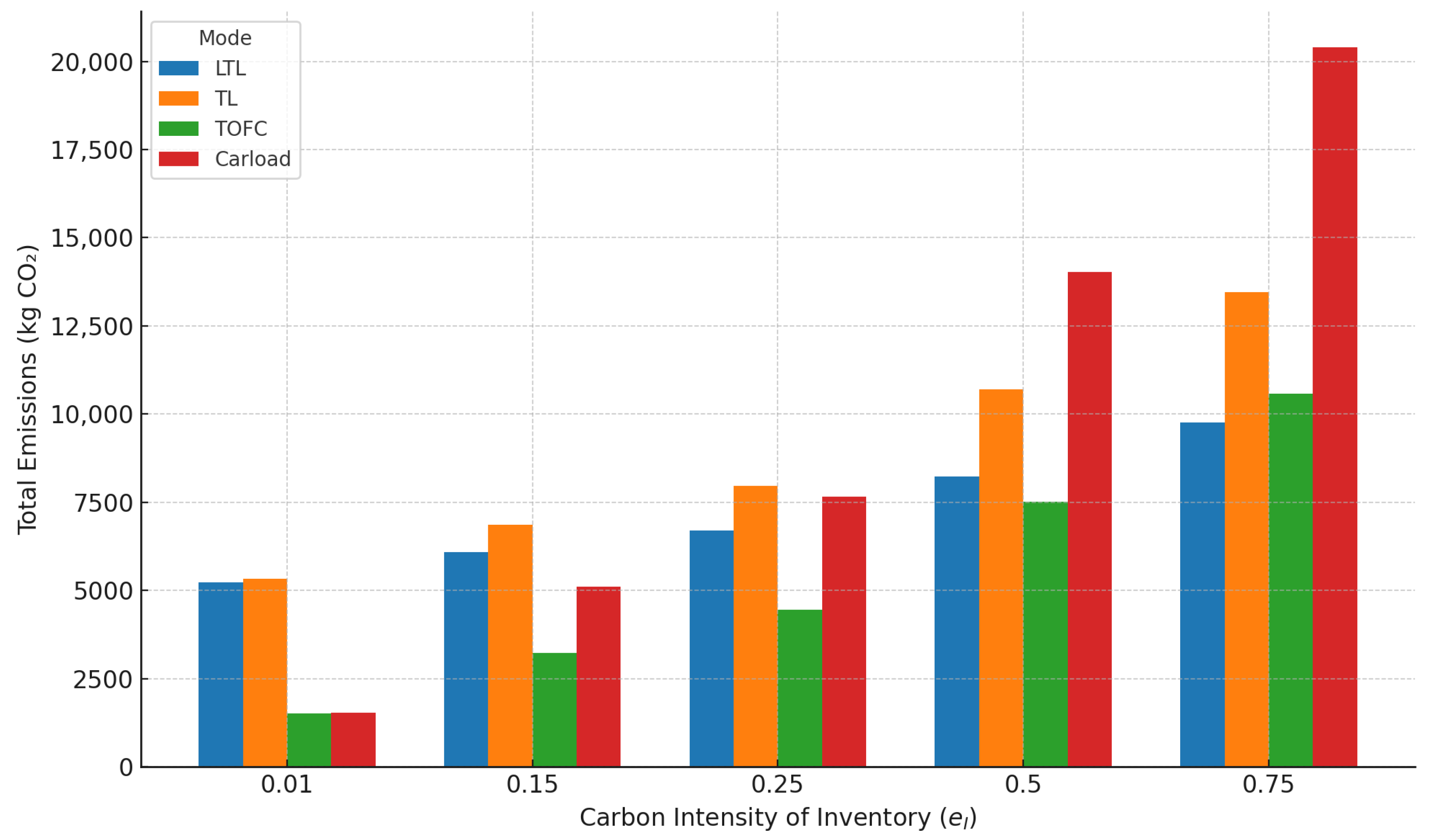
Figure 3 illustrates how the total emissions by mode were affected by increases in the carbon intensity of the inventory ($e_I$). While transportation emissions are typically the dominant source of logistics-related greenhouse gas emissions, this chart demonstrates that inventory-related emissions can become increasingly significant, particularly for slower modes of transportation that carry larger average inventory levels.

Slower modes such as carloads and TL tend to involve longer lead times and higher in-transit or buffer stock, making them more sensitive to changes in $e_I$. As the figure shows, the total emissions for these modes escalated rapidly with increases in the inventory carbon intensity. For example, at $e_I=0.75$, warehouse emissions accounted for approximately 94% of the total emissions for carloads and 61% for TL, overtaking transportation as the dominant emissions source. Even TOFC, which has relatively efficient transit emissions, saw its warehousing share rise from 8% at $e_I=0.01$ to nearly 87% at $e_I=0.75$.

By contrast, faster modes such as LTL are less sensitive to increases in $e_I$, since they tend to move goods more quickly and require less inventory buffering. For instance, the warehousing share for LTL rose from 1.2% to 47% as $e_I$ increased from 0.01 to 0.75.

Based on the parameters used in this analysis, values of $e_I$ between 0.01 and 0.25 corresponded to warehousing contributions of 1–35% of the total emissions for LTL and TL, consistent with the reported values of 11–30% that are typical for warehouse emissions across multiple industries, including CPG [6,7]. However, in sectors requiring specialized storage conditions—such as frozen foods, pharmaceuticals, or temperature-controlled products—$e_I$ can be considerably higher. These goods are often shipped via specialized modes due to their handling needs and shorter shelf lives, underscoring the importance of accounting for inventory emissions even when non-environmental factors drive such operational choices.

Firms facing high $e_I$ values can also take action on the warehousing side. Investments in energy-efficient buildings, improved insulation, high-performance cooling systems, and on-site renewable energy can reduce the effective carbon intensity of storage. This, in turn, can preserve the viability of slower, cost-effective modes like carloads, even under stricter sustainability requirements. Thus, Figure 3 highlights how the model supports a more holistic view of emissions management, enabling informed trade-offs across transportation, warehousing, and investment planning.

Such sensitivity analysis underscores the flexibility of our model as a managerial decision support tool, allowing exploration of how a broad range of operational parameters influence freight mode selection and inventory decisions. Managers can systematically vary critical inputs, such as annual demand, carbon budgets, transportation fuel efficiency, inventory holding costs, and warehousing emission factors, to observe how optimal strategies shift in response. For example, increasing annual demand typically encourages mode shifts toward more cost-effective, higher-capacity solutions such as rail or intermodal transport, at the cost of increased inventories. Conversely, tighter carbon constraints may favor lower-emission but potentially costlier transportation options. Improvements in transportation fuel efficiency or emissions intensity may allow managers to revert to faster, traditionally emission-intensive modes without violating carbon limits. Moreover, a high emissions factor for warehousing emphasizes the importance of faster delivery modes or enhanced warehouse management to minimize inventory holding periods and associated emissions. By evaluating such trade-offs across diverse scenarios, managers gain nuanced insights into the complex interplay between cost, emissions, inventory policy, and service levels. Ultimately, the model empowers firms to proactively prepare for policy changes, anticipate operational impacts, and align logistics strategies effectively with corporate sustainability objectives.

4.3. Managerial Insights

This paper’s analysis illustrates how incorporating carbon constraints into freight-mode decisions can alter traditional cost-minimizing solutions. Our results show that enforcing a voluntary carbon cap can force a shift away from purely cost-minimizing modes to those that balance economic efficiency with lower GHG emissions. Several recent trends underscore the importance of incorporating sustainability into freight decisions.

4.3.1. Stricter Policies and Stakeholder Mandates

Carbon Border Adjustment Mechanism (CBAM). The European Union’s CBAM [46] and similar initiatives effectively tax carbon-intensive products worldwide. Such policies ripple through global supply chains, leading shippers to reconsider mode selection, particularly for carbon-intensive trucking and long-haul shipping, when products cross regulated borders.

Corporate Net-Zero Targets. Many firms have adopted internal carbon budgets and science-based targets [47]. These self-imposed caps heighten the strategic importance of adopting cleaner freight modes and improving energy efficiency in warehousing, as demonstrated in our model’s trade-off between transport and inventory-related emissions.

4.3.2. Emergence of Low-Carbon and Alternative Fuel Technologies

Hydrogen and Electric Fleets. Technological advances in battery-electric and hydrogen fuel cell powertrains are emerging in both short-haul and long-haul freight, though adoption remains in the pilot stages [48]. Even modest improvements in the fuel efficiency parameter ($f_{m,T}$) can keep faster modes cost-competitive without breaching a carbon budget.

Cleaner Maritime and Rail Operations. Ocean shippers increasingly use slower steaming, alternative fuels (biofuels, LNG, and methanol), and improved hull designs to cut emissions [49]. Rail has also seen more significant deployment of hybrid-electric locomotives, enhancing rail’s emissions profile. Both developments can reduce the net emissions of slower modes and broaden their appeal under stricter carbon targets.

4.3.3. Balancing Transportation Versus Warehousing Emissions

Energy-Efficient Warehousing. Although transportation usually dominates total supply chain emissions, warehousing can become a significant source of carbon when more extensive safety stocks must be carried for slower modes. Current best practices include automated, high-density storage solutions and on-site renewable energy (e.g., rooftop solar), which reduce the per-unit warehousing emission factor ($e_I$).

Network Optimization and Collaborative Planning. Digital supply chain tools—such as real-time visibility platforms, predictive analytics, and digital twins—allow more accurate demand forecasting and dynamic inventory positioning, often reducing the total inventory in the system [50]. Lower inventory translates into fewer warehousing emissions, permitting more flexibility in choosing faster but potentially less fuel-efficient modes without exceeding a carbon budget.

4.3.4. Scenario-Based Decision Making Under Uncertainty

Volatile Lead Times and Disruptions. Port congestion, extreme weather events, and driver shortages can exacerbate lead time variance, making the choice between frequent, fast shipments and slower, more carbon-efficient modes more complex. Our model’s stochastic demand and lead time framework support scenario testing, enabling managers to anticipate how disruptions affect cost and carbon performance.

Carbon Pricing and Internal Shadow Costs. Even without formal carbon taxes, some companies apply an internal “shadow price” to emissions to future-proof against tighter regulations. Incorporating a notional carbon cost directly into inventory-transport optimization can add clarify when investing in low-carbon logistics solutions or purchasing carbon offsets is cost-effective.

4.3.5. Long-Term Decarbonization Strategies and Collaborative Initiatives

Carrier Engagement and Co-Innovation. Improving aerodynamic designs, rolling out electric or hydrogen trucks, and sharing route optimization data are proven ways to boost efficiency across the supply chain. Collaboration helps shippers and carriers meet internal carbon goals while maintaining service levels.

Standardizing Freight Emissions Measurement. Organizations such as the World Resources Institute and the World Business Council for Sustainable Development promote standardized frameworks (the GHG Protocol) to track emissions across supply chain partners. Widespread adoption simplifies benchmarking and fosters more transparent “green” freight tenders or carbon reduction alliances.

Network Restructuring and Multi-Echelon Systems. A single carbon budget applied to a multi-echelon network amplifies these trade-offs, especially for multi-product operations. Our approach can be extended to examine how distributing inventory across multiple regional facilities reduces long-haul emissions but increases warehousing carbon footprints at each node.

Overall, the continued tightening of emission regulations, rapid advancements in low-carbon freight technologies, and increasing sophistication of supply chain analytics are converging to reshape mode choice decisions. Managers must weigh costs, service levels, and a voluntary (or mandated) carbon cap as coequal factors. The model presented here offers a practical starting point for capturing these interdependencies. By systematically evaluating how emissions budgets interact with transportation costs, holding costs, and service requirements, firms can better align their inventory and transport strategies with economic and sustainability objectives.

5. Summary and Conclusions

• Key Contributions

The clarion call for action against climate change has many firms reexamining traditional supply chain decisions under the new lens of GHG emission mitigation. This paper provides a model that helps planners choose the appropriate freight mode when voluntary carbon constraints are in place.

Our model uses a continuous-review reorder-point stochastic inventory control context to compute the optimal lot size, reorder point, and mode choice for a given product and freight mode characteristics. Our model assumes a voluntary emissions constraint on total emissions from transportation and warehousing activities. Decisions are made through a comprehensive inventory-transportation cost framework that includes all relevant costs of the order management cycle—ordering, the holding cycle, safety, and in-transit inventory—and finally the cost of transportation. Our model accommodates various stochastic environments and product and freight mode characteristics.

The key finding of this paper, other than the methodology to evaluate mode choice, is that firms with voluntary constraints on emissions may be forced to choose modes of freight that do not have the lowest overall cost (because they violate carbon constraints). This either forces the firm to spend more on a mode with lower emissions or invest in trying to lower the emissions of the lowest-priced mode. There are multiple strategies for improving efficiency (the $f_{m,T}$): better-designed vehicles that use less fuel, optimizing the transport network, and efficient load planning that increases weight and cube utilization and reduces the number of trips. A second strategy is to switch fuels; moving to hybrid vehicles or those that run on bio-fuels also reduces $e_T$. A third strategy to reducing warehousing emissions ($e_I$) is to build energy-efficient warehouses that run on renewable fuels, such as solar, and make improvements that improve the energy efficiency of these buildings. These three strategies can have a significant impact on freight and warehousing emissions. Fourth, firms can also make gains by lobbying for emission cap legislation, where any savings below the cap can then be “traded” for revenue.

• Limitations

Despite providing a richer view of emission-aware logistics strategies, our model remains subject to several simplifying assumptions. We focused on a single-echelon, single-product system, which may not reflect the complexity of multi-echelon networks handling diverse product portfolios and multiple origins or destinations. Additionally, we treated the carbon budget as a hard constraint rather than a price-based mechanism (e.g., cap-and-trade or offset markets). Some firms may prefer to purchase additional carbon allowances rather than overhaul established transport arrangements, altering the cost-emissions trade-off. Lastly, the warehousing capacity was assumed to be unlimited, whereas in practice, physical constraints may impose further complications and costs.

• Directions for Future Research

Several promising paths extend beyond the scope of this paper. A multi-echelon version of the model would investigate how decentralized distribution centers collectively manage a shared carbon budget. Similarly, a multi-product setting would explore how firms allocate a single carbon pool among SKUs with differing demand volatility, weight, and service requirements. Introducing dynamic or rolling-horizon decisions could better capture real-world fluctuations in demand, lead times, or carbon price signals. Incorporating explicit carbon pricing or offset markets could also transform the carbon constraint into a cost element, potentially leading to more nuanced mode-switching decisions and providing deeper insights into the financial implications of various sustainability strategies. Finally, empirical validation with industrial case studies—particularly in industries vulnerable to tighter carbon regulations—would strengthen the practical relevance of our model.

• Concluding Remarks

In an era of growing climate policy stringency and heightened stakeholder scrutiny, logistics managers cannot ignore the emissions profiles of freight operations. Our model quantifies and compares how different modes, inventory policies, and warehouse configurations align with cost targets and carbon constraints. By shedding light on these trade-offs, we hope to empower organizations to design supply chains that are economically resilient and environmentally responsible. As carbon policies and technologies evolve, the integrated model proposed here will be invaluable in guiding the transition toward lower-carbon logistics networks.