Enhancing Driving Safety Evaluation Through Correlation Analysis of Driver Behavior

Abstract

This paper presents a method for evaluating driving behavior safety based on real-world urban driving data collected from on-road experiments. The aim of this study is to develop a comprehensive and interpretable evaluation framework to improve the identification and correction of unsafe driving behaviors, particularly in urban electric vehicle applications. Five driving behavior indicators were selected: average speed, speed fluctuation difference, acceleration range, speeding frequency, and speed change frequency. The Frequent Pattern Growth (FP-growth) algorithm was applied to model and analyze the hidden relationships between these indicators. Principal component analysis (PCA) was used to determine the weight of each indicator, resulting in a comprehensive safety evaluation method based on the correlation of driving behaviors. The findings reveal that unsafe driving behaviors often occur in combination, with speeding, rapid acceleration, and speed change frequency frequently coexisting on the same road segment, collectively influencing driving safety. The proposed evaluation method was validated through comparative analysis of driving safety scores across different drivers, providing a useful reference for improving and correcting unsafe driving behaviors.

1. Introduction

As urban traffic conditions become increasingly complex, driving behavior plays a critical role in road safety. Drivers are central to the traffic system, and unsafe driving behaviors—such as rapid acceleration, frequent deceleration, and speeding—are key contributors to traffic accidents [1,2,3,4]. These behaviors can be influenced by a range of factors, including vehicle performance characteristics, traffic flow, and driver habits. Particularly in real-world urban environments with frequent stops, variable speed limits, and high vehicle density, drivers may exhibit irregular or unsafe behavior patterns that require attention. Therefore, developing a scientifically sound and practical method to evaluate driving behavior safety can help provide timely feedback to drivers and reduce the likelihood of risk-inducing behaviors on the road.

Driving behavior has attracted growing international attention, as it reflects the continuous interaction between the driver, vehicle, and environment [5,6]. Recent studies have emphasized the impact of specific road contexts—such as proximity to intersections—on driving behavior. For instance, Tawfeek and El-Basyouny proposed a context identification layer in driver assistance systems to distinguish behavior near intersections [7], while their follow-up work further quantified behavioral differences during braking based on location, indicating drivers tend to behave more aggressively near intersections [8]. Driver behavior is fundamentally shaped by individual habits, skills, and internal states. To assess safety, driver profiling typically involves collecting vehicle dynamics data (e.g., speed, acceleration, and trajectory) over time and applying computational models for evaluation [9]. Driver behavior analysis typically involves identifying risky events, quantifying safe driving frequency, and evaluating safety based on driving strategies [10].

However, research on driving behavior safety evaluation still faces numerous challenges, and a unified evaluation framework has yet to be established [11]. To address this issue, some studies have focused on the correlation between different driving behaviors by mining in-vehicle data collected through traditional onboard recorders, such as vehicle speed and acceleration [12]. These works extract feature variables and utilize association analysis to explore frequent co-occurring patterns that reflect potential risk factors. Qu et al. and Kong used the NDS and USDOT datasets to extract association rules that reveal factors affecting crash severity and hidden links among travel behavior, road features, and speeding [13,14]. Sun and Das et al. applied the Apriori algorithm to explore associations between negligent behaviors and external factors, including fog visibility and poor lane-keeping, aiming to reduce road-departure crashes in low-visibility conditions [15,16].

In addition to the above correlation-based methods, another line of research explores scoring frameworks by selecting or designing driving behavior evaluation indicators. Scholars initially relied heavily on statistical questionnaires or direct feature screening from driving datasets to formulate scoring models for safety evaluation [17,18]. Faria et al. and Kinnear assessed driver behavior by combining questionnaires and driving simulations, aiming to support behavior classification and improvement [19,20]. However, such survey-based methods face limitations related to subjectivity and potential inaccuracies in driver-reported responses. To address this, Eusofe and Zhang applied the Analytic Hierarchy Process (AHP) and Principal Component Analysis (PCA) to perform more objective and efficient evaluation of driving behavior [21,22]. Nonetheless, methods like AHP may still introduce subjectivity in the weighting of indicators and fail to account for inter-indicator relationships.

To overcome the limitations of traditional evaluation methods, recent studies have increasingly embraced machine learning algorithms to construct data-driven, objective evaluation models. For instance, Chong et al. proposed a rule-based neural network model to simulate drivers’ longitudinal and lateral control behaviors in safety-critical scenarios [23]. While powerful, such models often depend on carefully selected fuzzy membership functions, requiring multiple rounds of validation. An increase in feature variables leads to more fuzzy rules, resulting in higher computational complexity and longer runtimes [24]. Yu et al. utilized the random forest algorithm to model braking behavior and computed feature importance scores to identify dominant factors [25]. Their findings also highlighted that model performance was sensitive to the training-test ratio and number of decision trees used. In addition, a variety of other machine learning methods—such as Support Vector Machines (SVM), XGBoost, Classification and Regression Trees, and Multilayer Logistic Regression—have been applied in driving behavior safety research to enhance model adaptability and robustness [26,27,28,29].

Although progress has been made in evaluating driving behavior and correlations, existing methods face several limitations. In particular, machine learning models are sensitive to data partitioning and struggle with complexity when handling large-scale, high-dimensional driving data [30,31,32]. This leads to longer computation times and higher demands on computer performance. Regarding driving behavior correlation analysis, traditional in-vehicle data collection systems have been extensively applied in analyzing driver behavior, and recent developments such as connected vehicle technologies (e.g., V2I communication) have further enhanced their data acquisition capabilities [33]. However, these systems may still face limitations when it comes to capturing high-frequency, multidimensional signals—such as real-time trajectory tracking and rapid behavioral transitions—especially under complex urban traffic conditions. 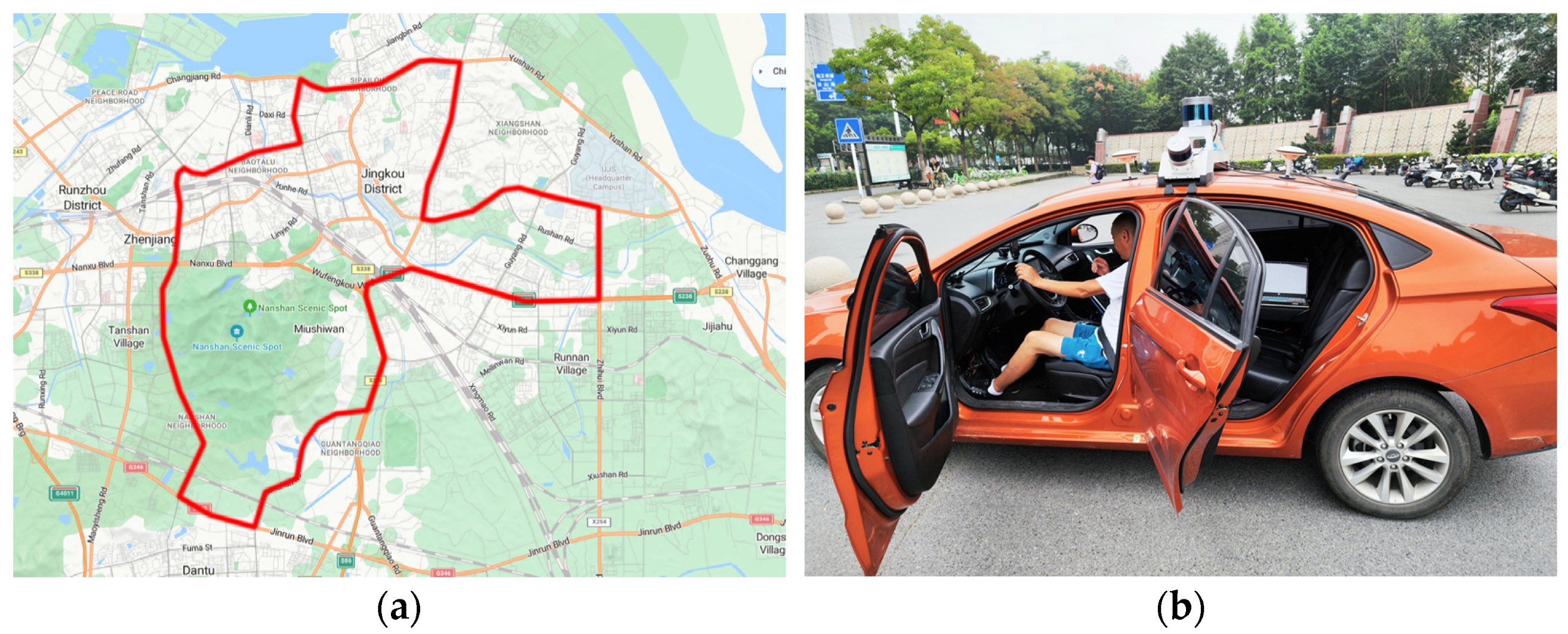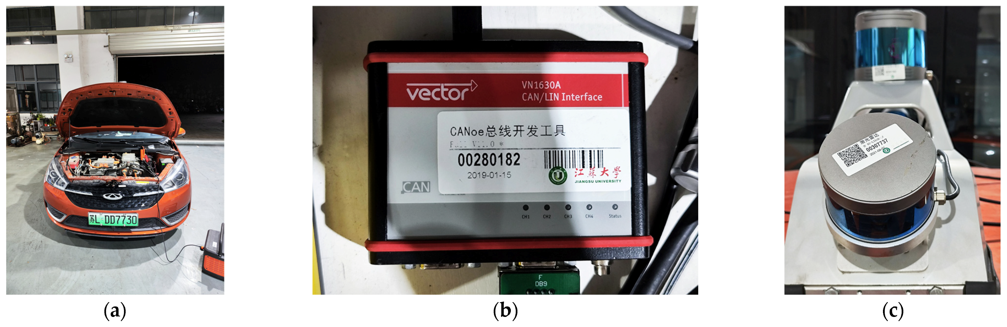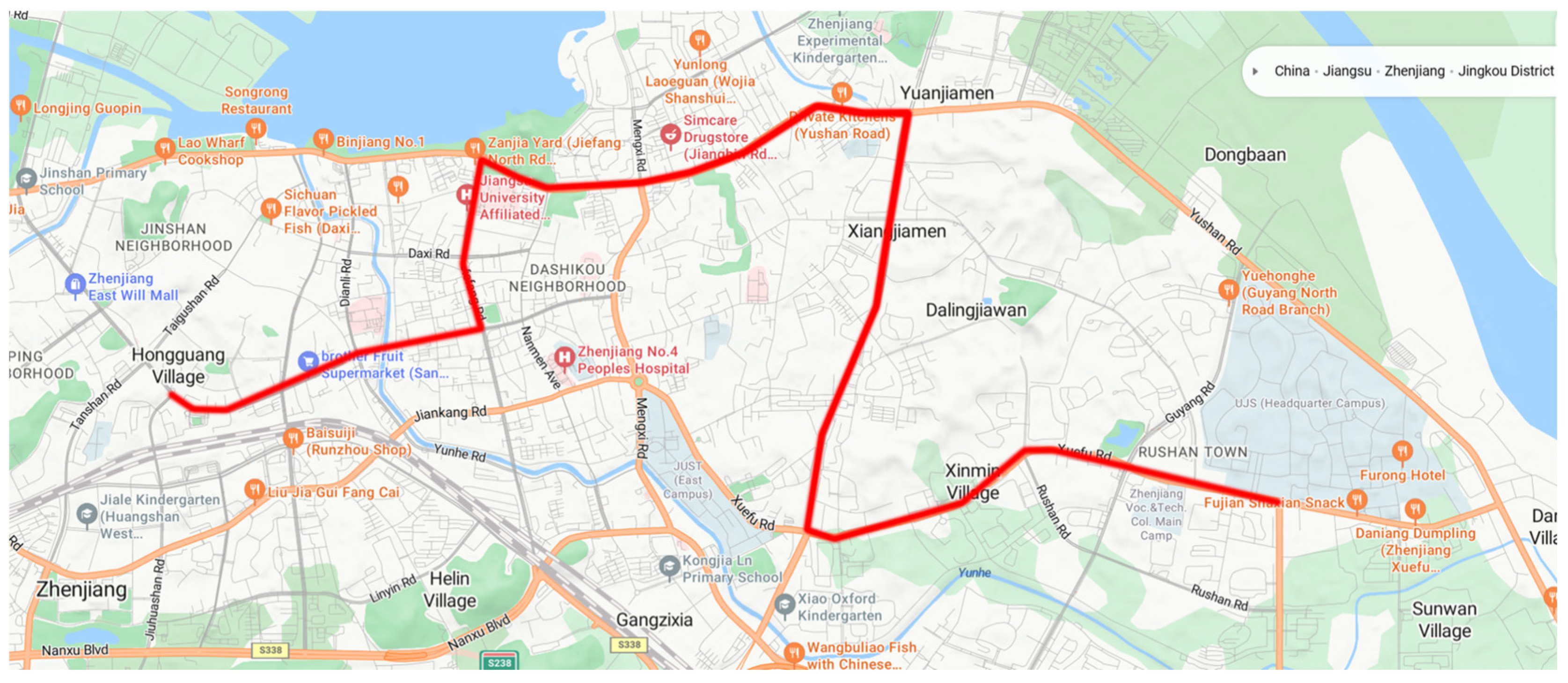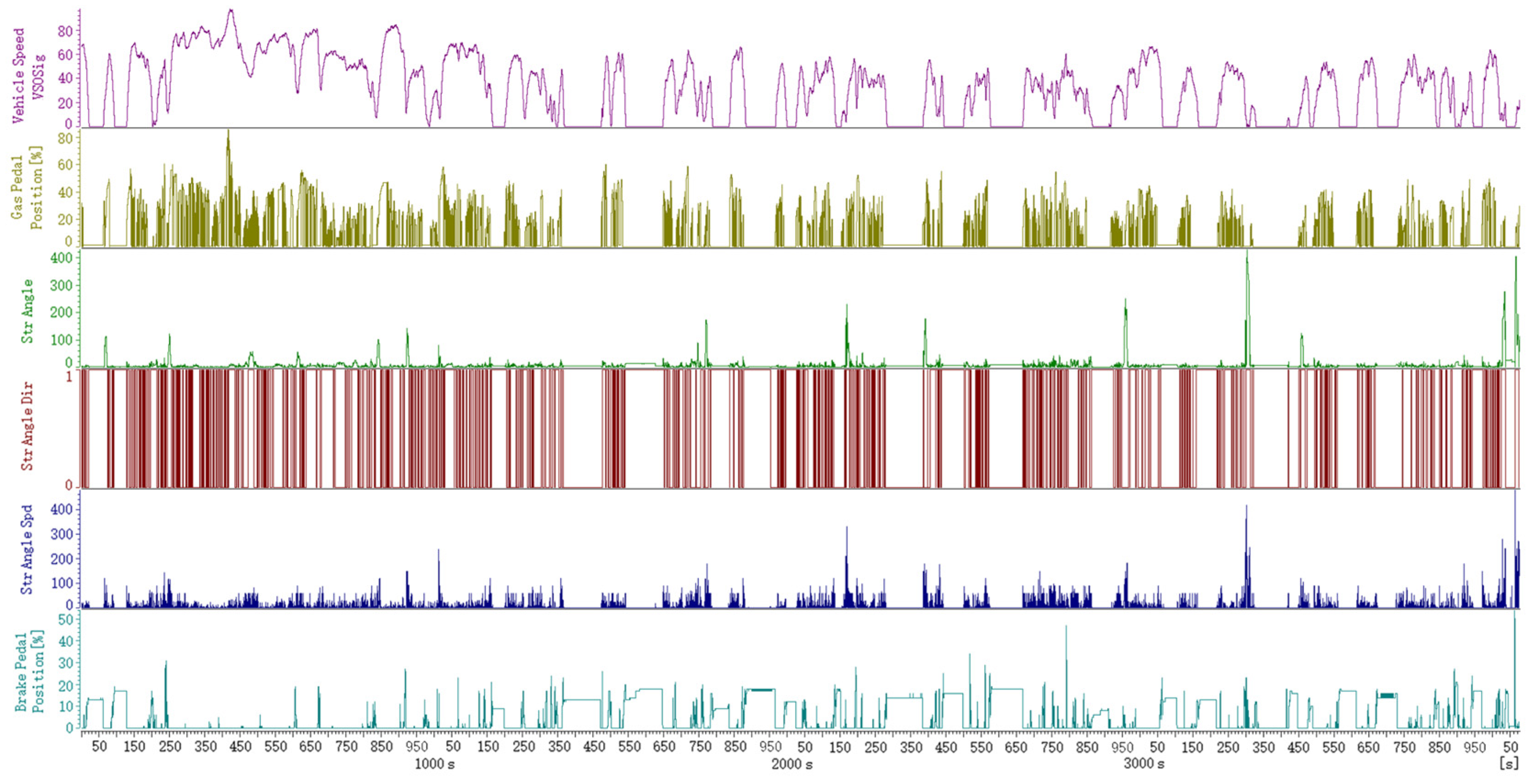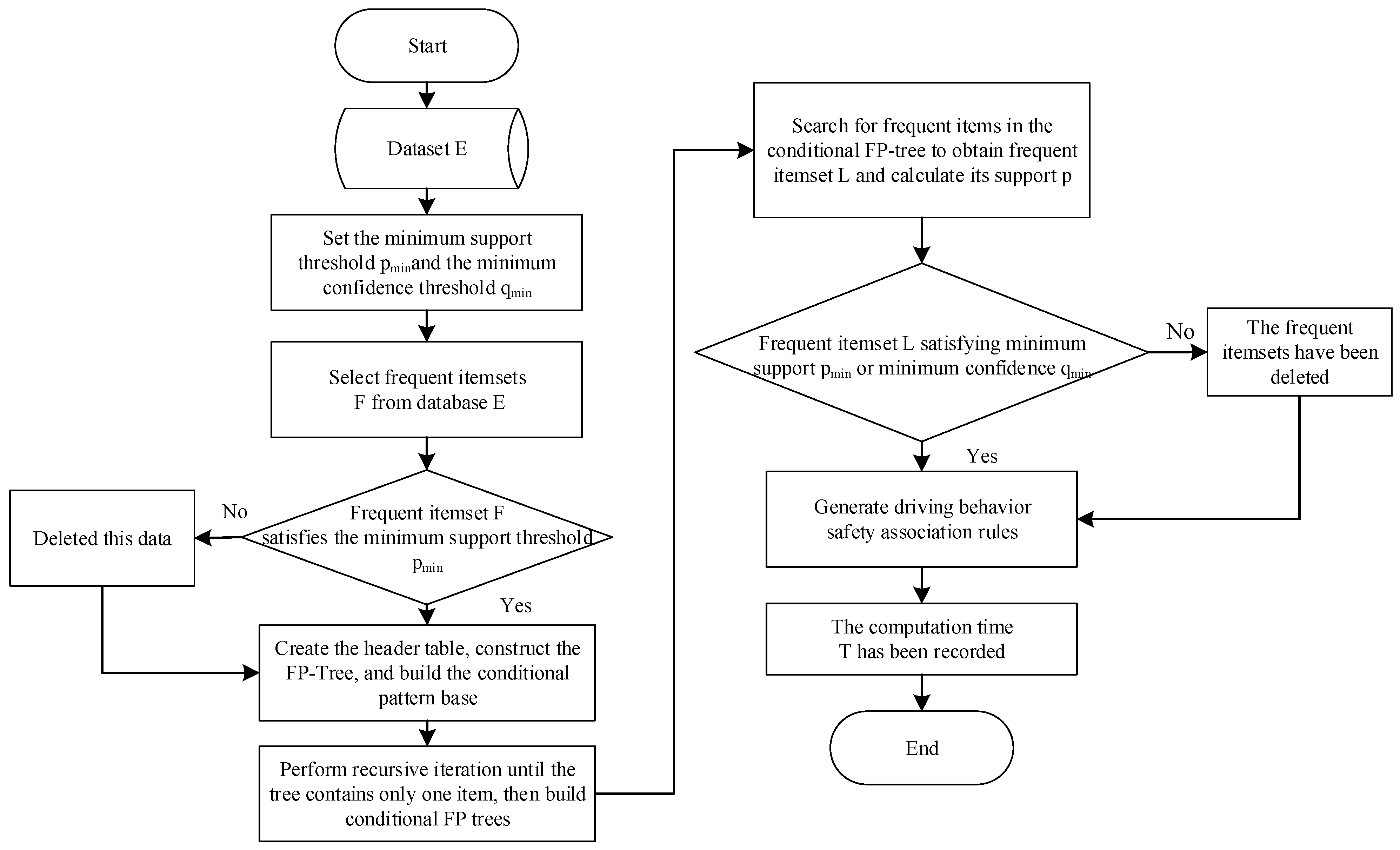Moreover, Apriori repeatedly rescans high-frequency datasets to compute itemset support, generating excessive candidate sets and leading to redundancy in indicator selection [34,35]. Therefore, this study uses high-frequency urban driving data from real-world experiments—including vehicle signals and GPS-inertial information—to enable precise vehicle localization and in-depth safety analysis. By setting thresholds for driving behavior safety evaluation indicators, this study applies the Frequent Pattern Growth (FP-growth) algorithm to driving behavior correlation analysis for the first time [36]. Unlike Apriori, the FP-growth algorithm constructs a compact FP-tree to efficiently mine frequent itemsets without repeated database scans. Combined with threshold-based indicator weighting, it enables quantitative evaluation of individual driving behaviors, facilitating clear differentiation between safe and unsafe drivers. This approach enhances both accuracy and interpretability compared to traditional machine learning models.

This study aims to uncover latent relationships among unsafe driving behaviors by addressing the limitations of prior research. Leveraging high-frequency real-world driving data from urban environments, it employs the FP-growth algorithm to mine associations among key safety evaluation indicators. Unlike traditional methods that focus solely on individual indicators or rely heavily on machine learning black-box models, this study introduces an interpretable pattern-mining framework that integrates FP-growth with threshold-based scoring to uncover co-occurring risk behaviors. This approach enables both quantitative safety evaluation and transparent behavioral rule discovery, which is rarely addressed in prior driving behavior studies. Accordingly, this study proposes a method to evaluate and enhance driving behavior with the aim of improving road safety. 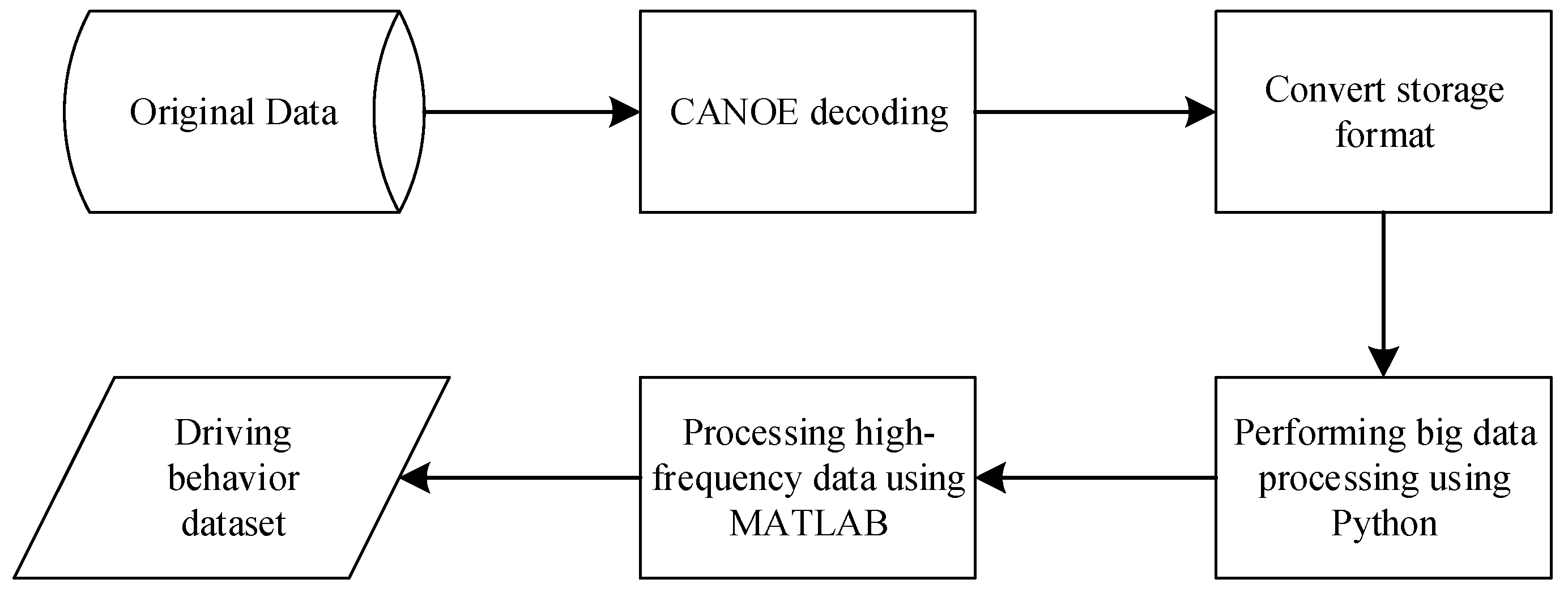The remainder of this paper is organized as follows: Section 2 describes the data collection and preprocessing procedures, as well as the selection of safety evaluation indicators, correlation modeling, and the proposed evaluation framework. Section 3 presents a comparative analysis using driver behavior data and safety scores to validate the method. Section 4 concludes with the study’s key findings and limitations.

2. Materials and Methods

2.1. Experiment

2.1.1. Experimental Design

To examine the inherent correlations in drivers’ driving behavior characteristics and assess the safety of their driving behavior, the research team conducted real-world experiments in designated urban and suburban areas of Zhenjiang City. Figure 1 illustrates the experimental route, spanning a total distance of 32.9 km, with both the starting and ending points situated at the main gate of Jiangsu University. The route passes through typical urban facilities, such as commercial squares, schools, and hospitals, known for their traffic congestion.

All participating drivers were informed that their driving behavior would be recorded, and consent was obtained prior to data collection. To avoid influencing driver behavior, the specific objectives of the study were not disclosed. During the experiments, all drivers followed a fixed route under real-world traffic conditions, guided by a navigation system. No additional driving instructions or interventions were provided, allowing drivers to operate the vehicle according to their usual habits while ensuring route consistency across participants.

A total of 36 drivers participated in the experiment, comprising 26 males and 10 females, aged between 26 and 57 years old, with driving experience spanning 3 to 30 years. All drivers exhibited corrected visual acuity of 1.0 or higher, maintained good physical health, and lacked a significant accident history, showcasing their capability to independently complete the driving test. Descriptive statistics of driver characteristics are presented in

Table 1. Distribution of drivers by age group and gender.

Statistical Variables	Stratification	Number of Drivers	Percentage (%)
Age	Young Adults (<30 years old)	21	58.33%
	Middle-aged (≥30 years old)	15	41.67%
Gender	Male	26	72.22%
	Female	10	27.78%

.

The experiment was conducted using a manually driven fully electric vehicle (FEV), specifically a Chery Arrizo modified for data collection and analysis. CANOE onboard signal acquisition equipment was installed on the electric vehicle to capture signals during each trip, including time, vehicle speed, percentage of accelerator and brake pedal travel, steering wheel rotation, angle, and velocity. Additionally, the GPS radar inertial navigation system was utilized to determine the experimental vehicle’s driving position, capturing parameters like latitude, longitude, and time. Figure 2 displays the experimental equipment. The radar inertial navigation equipment is used to acquire the vehicle’s latitude and longitude information.

2.1.2. Data Collection

Each round trip, forming a closed-loop route where the starting point and ending point coincide, constituted one set of trips. Trip data were gathered from various drivers utilizing the same electric vehicle on identical routes for a period of up to 5 months, yielding a total of 306 datasets. Among these, 225 datasets were amassed during morning and evening rush hours, with an additional 81 datasets collected during midday off-peak hours. It is important to note that this study exclusively focuses on the 225 rush-hour datasets, as these reflect more dynamic and safety-critical traffic conditions. The off-peak datasets were not used in the subsequent modeling and evaluation, but are retained for potential future work. The heightened traffic density during urban rush hours creates a more intricate road environment, predisposing to the occurrence of hazardous driving behaviors. Moreover, varying speed limits between urban and suburban roads result in disparate threshold values for subsequent driving behavior evaluation indicators, complicating encoding standardization. Thus, to conduct a more precise and efficient examination of the inherent correlation among driving behaviors, this study concentrated on the 225 datasets obtained during urban rush hours (the urban road segment is shown in Figure 3). During peak hours, the 36 drivers completed a minimum of 5 driving sessions and a maximum of 9 sessions, with an average of approximately 6 sessions. The urban road segment is based on the actual driving route, which includes roads passing through typical urban facilities that are prone to congestion, such as commercial plazas, schools, and hospitals. The entry point into the urban road segment is marked by the intersection of Jiuhua Mountain Road and Zhongshan West Road, with the stopping point at the main gate of Jiangsu University. The route passes through Zhongshan West Road, Jiefang Road, Dongwu Road, Yushan Road, Jiaoshan Road, and Xuefu Road. Figure 4 illustrates the signal source code acquired by the CANOE acquisition device, as exemplified by a trip on 27 September 2023.

2.1.3. Data Processing

To facilitate visual analysis and reduce file size, the high-frequency driving data were downsampled to 0.1-s intervals. This interval was selected considering human reaction times (typically 0.15–0.4 s) and the need to preserve key fluctuation characteristics for safety analysis. For parameters sampled at 0.01-s intervals (e.g., speed and acceleration), every 10th point was retained to avoid smoothing out critical anomalies such as sudden acceleration or deceleration. MATLAB R2022b is utilized to process the high-frequency data offline, offering better visualization and extraction of temporal features that are difficult to observe using tabular methods, illustrated in Figure 5.

Abnormal data filtration is conducted utilizing a sliding window approach with a standard window size of 5 s. The pandas library in Python programming software (version 3.12.1) is used to read the Excel data, as its packages provide flexible support for handling raw data formats and sequence operations. Trip data is organized chronologically based on the travel dates. The maximum value from the time column is extracted to establish the upper time period limit. Time periods then are delineated and their frequencies are recorded, with each minute constituting a distinct period. A short trip is characterized as the distance covered within a single minute.

2.2. Selection of Evaluation Indicators

Driver behavior is reflected through control of vehicle dynamics such as acceleration, braking, and steering, which directly affect vehicle motion. Among these, speed and acceleration are key indicators for behavior analysis and are closely linked to traffic accident risks [37]. Given the link between driver behavior and accident risk, this study assessed safety based on the frequency of hazardous events. Vehicle motion data were collected via the CANOE onboard system, with emphasis on speed-related variables. Drawing on prior studies and data characteristics, five evaluation indicators were selected: average speed, speed fluctuation difference, acceleration range, speeding frequency, and speed change frequency. Thresholds were defined for these indicators to identify unsafe driving behaviors [38,39,40,41,42].

2.2.1. The Threshold for Average Speed

In this paper, the average speed refers to the arithmetic mean of all available speed readings within a given urban road segment. We have used time-averaged speed, which involves sampling vehicle speeds over a defined time interval and calculating the average of all speed data points. This definition ensures the representativeness of the data and effectively reflects the overall driving conditions within the segment. The analysis of average speed data for average speed of trips reveals the distribution of speeds, as depicted in Figure 6. Remarkably, the percentage of average speeds falling within the range of 20 to 25 km/h (12.43 to 15.53 mph) is remarkably high at 58.75%, indicating a notable concentration of vehicle speeds within this interval. In contrast to the CATC standard for urban road conditions, specifying an average speed of 29 km/h (18.02 mph), the calculation of the average speed threshold for speeding employs the following formula, denoted as $E_{\overline{V}}$:

$$E_{\overline{V}}=E_M+1.5E_N$$

(1)

where $E_M$ symbolizes the 75th percentile of the total distribution of average speeds across all samples; $E_N$ represents the interquartile range, denoting the difference between the 75th and the 25th percentiles of the total distribution of average speeds across all samples.

Figure 7 supplements the analysis with a box plot that elucidates the average speeds during morning and evening peak hours in urban areas. As shown in the figure, the distribution of average speeds on urban roads indicates that the majority of drivers have speeds concentrated within the range of 20–25 km/h (12.43–15.53 mph), with a relatively small interquartile range (IQR). The 75th percentile speed (24.62 km/h, 15.29 mph), used as the threshold, better reflects the safety risks associated with typical driving behaviors and is less influenced by extreme outliers. It effectively captures the behavioral characteristics of the primary group of drivers. In this specific context, $E_M$ = 24.62 km/h (15.29 mph), $E_N$ = 4.17 km/h (2.59 mph), $E_{\overline{V}}$ = 31 km/h (19.26 mph).

2.2.2. The Threshold for Speed Fluctuation Range

According to early research by Solomon and the Accident Research Centre at Monash University, the greater the difference between vehicle speed and average speed, the higher the accident rate. Therefore, the difference between the maximum speed and the average speed during vehicle operation can typically reflect the driver’s driving tendencies. This is particularly effective in representing hazardous driving behaviors under complex road conditions. The larger the difference, the less safe the driving behavior. The threshold for speed fluctuation range, denoted as $E_w$, is defined as the difference between the maximum vehicle speed and the average vehicle speed during the journey. This definition is formulated as:

$$E_w=E_{Vmax}-\overline{V}$$

(2)

where $E_w$ symbolizes the threshold for speed fluctuation range; $E_{Vmax}$ represents the maximum vehicle speed; $\overline{V}$ represents the average vehicle speed.

Considering the maximum speed limit of 70 km/h (43.5 mph) on urban roads and an average vehicle speed of 23 km/h (14.29 mph) in this study, we establish the speed fluctuation difference threshold at 47 km/h (29.2 mph). Any value surpassing this threshold indicates unsafe driving.

2.2.3. The Threshold for Acceleration Range

The acceleration variation across all trips was computed, and the results are presented in Figure 8, with each trip plotted on the horizontal axis and its corresponding acceleration-deceleration range on the vertical axis. The analysis reveals a predominant concentration of acceleration around 2 m/s² (6.56 ft/s²), while deceleration primarily falls within the range of 2.75 m/s² (9.02 ft/s²). Considering the acceleration variation and testing conditions, the threshold value $E_a$ is selected. The data collected for this study were conducted under full load conditions with air conditioning during the summer. Therefore, the values for maximum acceleration and maximum deceleration were determined based on the air conditioning operating conditions in the U.S. EPA test procedure (SFTP-SC03) [43]. Considering these conditions, the maximum acceleration is set at 2.28 m/s² (7.48 ft/s²) and the maximum deceleration at −2.73 m/s² (−8.96 ft/s²). Any acceleration exceeding the maximum or deceleration below the maximum is considered to exceed the threshold. As a result, the acceleration range threshold is established at 5.01 m/s² (16.44 ft/s²).

2.2.4. The Threshold for Speeding Frequency

Considering the experimental road conditions, the urban road speed limit is set at 60 km/h (37.28 mph), with a speeding time window of 4 s. Let $E_n$ denote the threshold value for speeding frequency, indicating that any value exceeding 0 indicates occurrences of speeding. Figure 9 depicts the proportion of speeding frequency, revealing that the majority of urban speeding incidents fall within 80 km/h, concentrated mainly in the range of 60–65 km/h (37.28–40.39 mph).

2.2.5. The Threshold for Speed Change Frequency

Frequent changes in vehicle speed refer to the driver’s repeated speed adjustments (continuous acceleration and braking), which differ from sudden speed changes caused by responding to unexpected situations or the unstable operation of novice drivers. Based on the short trip segmentation per minute outlined in Section 2.3, and supported by the literature and real-world vehicle data, it is assumed that the acceleration variation induced by speed change typically remains within 1 m/s² (3.28 ft/s²) [44]. The speed change frequency is denoted as follows:

$$E_f=Q/T$$

(3)

where $E_f$ represents the speed change frequency; Q denotes the number of speed changes; T represents the unit time (in minutes).

By setting a threshold of 1 shift per minute for speed change frequency, surpassing this threshold indicates frequent speed change behavior, which is deemed unsafe driving.

2.3. Modeling the Correlation of Driving Behavior

2.3.1. Encoding of Evaluation Indicator Data

In this study, encoding refers to mapping each evaluation indicator to a discrete numeric value based on its threshold. This transformation enables the FP-growth algorithm to process diverse driving behavior indicators in a unified format.

For each trip, if a specific indicator exceeds its predefined threshold, it is encoded as a distinct item: e.g., {1} for average speed, {2} for speed fluctuation difference, etc. Indicators not exceeding the threshold are omitted. The trip dataset is then represented as a set of triggered events, such as {1, 2, 3}, where each number corresponds to an unsafe behavior type. For example, if the average speed exceeds 31 km/h, the segment is encoded as {1}; otherwise, it remains an empty set.

The encoding rules for the five driving behavior indicators—average speed, speed fluctuation difference, acceleration range, speeding frequency, and speed change frequency—are shown in

Table 2. Encoding of driving behavior evaluation indicators and their corresponding thresholds.

Encoding	Driving Behavior Evaluation Indicators	Threshold
1	Average speed	$E_{\overline{V}}$
2	Speed fluctuation difference	$E_w$
3	Acceleration range	$E_a$
4	Speeding frequency	$E_n$
5	Speed change frequency	$E_f$

. Each trip’s indicator parameters are then converted into corresponding numeric sets based on these rules.

2.3.2. Modeling Using FP-Growth Method

Association rules are widely used in data mining to identify inherent relationships among variables within large datasets. In this study, they are employed to reveal co-occurrence patterns among the five driving behavior indicators. The FP-growth algorithm, known for its efficiency in mining association rules [45], requires only two scans of the database, significantly reducing computation time. It is therefore adopted here to analyze the correlation between unsafe driving behaviors.

The correlation between evaluation indicators of driving behavior can be represented as $\alpha \Rightarrow \beta$, satisfied: $\alpha \subset H$, $\beta \subset H$ and $\alpha \cap \beta =\varnothing$, where $\alpha$ represents the antecedent indicators and $\beta$ represents the consequent indicators in the association rule.

The correlation of driving behavior evaluation indicators $\alpha \Rightarrow \beta$ has a support level of p, referring to the proportion of the itemset within the entire set of driving behavior evaluation indicators. The confidence level of $\alpha \Rightarrow \beta$, denoted as q, refers to the probability that the evaluation indicator itemset contains $\alpha$ while also containing $\beta$. Actually, it represents the conditional probability, denoted as $P(\beta |\alpha )$.

Support, represented as p, is expressed as:

$$support(\alpha \Rightarrow \beta )=P(\alpha \cup \beta )$$

(4)

Confidence, denoted as q, is expressed as:

$$\mathit{confidence}(\alpha \Rightarrow \beta )=P(\beta |\alpha )=support(\alpha \cup \beta )/support(\alpha )$$

(5)

The lift of driving behavior evaluation indicators represents the extent to which the occurrence of itemset $\alpha$ increases the probability of itemset $\beta$. The lift is expressed as:

$$\mathit{lift}(\alpha \Rightarrow \beta )=\mathit{confidance}(\alpha \Rightarrow \beta )/support(\beta )$$

(6)

An uplift of 1 indicates independence between the antecedent and consequent. An uplift greater than 1 signifies positive dependence, where the antecedent and consequent appear together more frequently than expected, while an uplift less than 1 indicates negative dependence, where they appear together less frequently than expected.

The computational process of FP-growth is illustrated in Figure 10.

2.4. Methodology for Evaluating Driving Behavior Safety

The conclusions derived from the correlation analysis of driving behavior in the third section reveal the interconnected nature of unsafe driving behaviors. Speeding, sudden acceleration, and frequent speed change often occur simultaneously during a journey, collectively affecting driver safety. Consequently, this study assesses driving behavior safety by analyzing the correlation among safety evaluation indicators. The significance of each evaluation indicator parameter for road traffic safety varies, thus influencing the rationality and scientific validity of the evaluation results based on the assigned indicator parameter weights. This paper employs the Statistical Product and Service Solutions (SPSS Statistics version 26.0) software package for principal component analysis to determine the weight factors of evaluation indicators, where its integrated statistical tools allowed for direct database import and efficient factor extraction [46].

2.4.1. Principal Component Analysis

This section primarily outlines the procedural steps of PCA implementation using SPSS. Initially, the dataset of safety evaluation indicators for driving behavior is imported into the SPSS software. Five evaluation indicator variables undergo standardization. Subsequently, the standardized variables undergo dimensionality reduction and factor analysis. The Kaiser-Meyer-Olkin (KMO) measure and Bartlett’s test of sphericity are then utilized to evaluate the appropriateness of Principal Component Analysis (PCA). If the KMO value exceeds 0.5 and Bartlett’s test significance level is below 0.05, PCA is considered suitable. Finally, PCA is conducted with the maximum number of iterations set for convergence. Outlier results are addressed by opting for the maximum variance and rotation solution. The factor score coefficient matrix is presented, with coefficients arranged in descending order to derive the results of principal component analysis. The extracted factor score matrix from SPSS serves as the foundation for computing the standardized scores of each evaluation indicator. These standardized scores are integrated through a weighted combination to construct the final comprehensive scoring model, as introduced in Section 2.4.2.

Table 3. Explained variance and cumulative contribution rates for each principal component.

Component	Initial Eigenvalue			Extracted Loadings Sum of Squares			Rotated Loadings Sum of Squares
	Total	Variance Percentage	Cumulative Percentage	Total	Variance Percentage	Cumulative Percentage	Total	Variance Percentage	Cumulative Percentage
1	1.934	38.686	38.686	1.934	38.686	38.686	1.895	37.896	37.896
2	1.393	27.866	66.552	1.393	27.866	66.552	1.433	28.656	66.552
3	0.897	17.937	84.489	/	/	/	/	/	/
4	0.478	9.568	94.056	/	/	/	/	/	/
5	0.297	5.944	100.000	/	/	/	/	/	/

and

Table 4. Rotated component matrix showing factor loadings of standardized evaluation indicators.

Standardized Evaluation Indicators	Component 1	Component 2
Zscore (Average speed)	0.773	−0.085
Zscore (Speed change frequency)	−0.159	0.866
Zscore (Speed fluctuation difference)	0.649	0.395
Zscore (Acceleration range)	−0.319	0.668
Zscore (Speeding frequency)	0.888	0.181

display the variance and cumulative contribution rates of each component derived from the principal component analysis conducted through SPSS software. Figure 11 illustrates the scree plot, while Figure 12 depicts the score plot. Table 3 indicates that the cumulative contribution rate of the initial two components amounts to 66.552%. Given the criterion of a cumulative contribution rate exceeding 60%, the selection of the first two components as characteristic parameters is justifiable. Similarly, Figure 11 illustrates that the eigenvalues of the initial two components exceed 1. The figure also visually demonstrates a distinct inflection point after the second component, reinforcing the decision to retain only the first two for dimensionality reduction. Consequently, adhering to the criterion of eigenvalues surpassing 1, the first two components can be selected. Thus, the eigenvalues of the first two principal components are utilized for weighting calculation. Figure 12 reveals partially overlapping black and red clusters, signifying their proximity and substantial similarity, aligning with the relative correlation of driving behavior evaluation indicators. This supports the interpretability of the component space and validates the use of PCA for grouping driver behavior patterns. To provide further clarity on the factor extraction process, the rotated component matrix is now included in

Table 5. Rotated component matrix for the two selected principal components. Rotation converged in 3 iterations.

Standardized Evaluation Indicators	Component 1	Component 2
Zscore (Average speed)	0.721	−0.290
Zscore (Speed change frequency)	0.081	0.877
Zscore (Speed fluctuation difference)	0.732	0.205
Zscore (Acceleration range)	−0.127	0.730
Zscore (Speeding frequency)	0.904	−0.066

. As shown, the loadings after applying the Varimax rotation method converged after three iterations. This rotated matrix supports the interpretability of the factor structure and confirms the validity of retaining two components. Each evaluation indicator shows a stronger loading on one of the components, enhancing the robustness and clarity of the component interpretation.

2.4.2. Calculation of Weights

Based on the principal component analysis results described in Section 2.4.1, the factor scores of each evaluation indicator are obtained through standardization and dimensionality reduction. To integrate these indicators into a unified safety score, a standardized composite weighting method is applied. The standardized scores are calculated using the following equation:

The coefficients F in the linear combination are computed as follows:

$$F={\displaystyle \frac{Z}{SQRT}}$$

(7)

where Z represents the standardized number, and SQRT represents the square root of the eigenvalue corresponding to the standardized number.

The coefficients K in the comprehensive scoring model in

Table 6. Principal component loading matrix: standardized coefficients of evaluation indicators.

Evaluation Indicators	Coefficient F1	Coefficient F2
Average speed	0.555675286	−0.071816885
Speed change frequency	−0.114596187	0.734067034
Speed fluctuation difference	0.466918727	0.334565335
Acceleration range	−0.229585668	0.566191757
Speeding frequency	0.638255445	0.153234641

are calculated as follows:

$$K={\displaystyle \frac{100S_1\cdot F_1+100S_2\cdot F_2}{S_1+S_2}}$$

(8)

F₁ and F₂ represent the standardized scores of the first and second principal components, respectively. These scores are derived from Principal Component Analysis (PCA) applied to the normalized driving behavior indicators (e.g., average speed, acceleration range); S₁ and S₂ denote the variance contribution rates of the respective principal components. These are obtained from the eigenvalue decomposition and indicate how much information each component captures from the original data. The formula computes the composite weight coefficient K, which reflects the overall contribution of the principal components and is used to weight their influence in the final scoring model (Equation (9)).

The comprehensive score coefficient K in

Table 7. Composite score coefficients and normalized weights for safety evaluation indicators.

Evaluation Indicators	Composite Score Coefficient K	Weighting of Evaluation Indicators R
Average speed	29.29385111	0.2
Speed change frequency	24.0746952	0.16
Speed fluctuation difference	41.15011377	0.28
Acceleration range	10.36136997	0.07
Speeding frequency	43.51727489	0.29

is normalized to derive the evaluation index weight R. Consequently, the safety evaluation indicator scores for driving behavior are established as follows:

$$E_s=0.2E_{\overline{V}}+0.28E_w+0.07E_a+0.29E_n+0.16E_f$$

(9)

3. Results and Discussion

3.1. Analysis of Correlation in Driving Behavior

3.1.1. Analysis of Driving Behavior Among All Drivers

To streamline data modeling and analysis, a minimum support threshold of 10% and a minimum rule confidence of 50% are established. The FP-growth algorithm is employed for data modeling, to execute the model, and to generate the results. Compared to the traditional Apriori algorithm, which repeatedly scans the dataset and generates a large number of candidates sets, FP-growth constructs an FP-tree and mines frequent patterns without candidate generation, offering significant computational advantages.

In this study, both algorithms were applied to the same encoded driving behavior dataset and yielded consistent association rules, demonstrating equivalence in logical output. However, the FP-growth method achieved over fivefold faster processing, reinforcing its suitability for high-frequency driving behavior analysis. This comparison illustrates the novelty and practicality of adopting FP-growth in structured behavioral safety evaluation. The top two and top three association rules between evaluation indicators based on confidence percentages are identified and prioritized, as depicted in

Table 8. Association rules among evaluation indicators of driving behavior for all driver groups.

Rules	Antecedent	Consequent	Support (%)	Confidence (%)	Lift
1	3	5	56.25	97.83	1.168
2	3	4	51.25	89.12	0.99
3	5	4	73.75	88.06	0.98
4	4	5	73.75	81.94	0.978
5	5	3	56.25	67.16	1.168
6	4	3	51.25	56.94	0.99
7	3–4	5	50	97.56	1.165
8	3–5	4	50	88.88	0.988
9	4–5	3	50	67.80	1.179
10	3	4–5	50	86.96	1.179
11	5	3–4	50	59.70	1.165
12	4	3–5	50	55.55	0.986

. Table 8 reveals 12 association rules involving acceleration range, speeding frequency, and speed change frequency evaluation indicators, while Figure 13 illustrates the strength of these association rules. However, association rules involving average speed and speed fluctuation difference are not statistically significant. This may be attributed to lower trip average speed during urban morning and evening peak road conditions, resulting from traffic flow constraints and limited variation in speed fluctuation difference.

3.1.2. Analysis of Driving Behavior Among Drivers of Different Ages

Analysis of Figure 14 and

Table 9. Association rules among evaluation indicators of driving behavior for young driver group.

Rules	Antecedent	Consequent	Support (%)	Confidence (%)	Lift
1	3	5	65.31	100	1.043
2	3	4	59.19	90.63	1.033
3	5	4	83.68	87.23	0.994
4	4	5	83.68	95.35	0.994
5	5	3	65.31	68.09	1.043
6	4	3	59.19	67.44	0.906
7	3–4	5	59.18	100	1.043
8	3–5	4	59.18	90.63	1.033
9	4–5	3	59.18	70.73	1.083
10	3	4–5	59.18	90.63	1.083
11	5	3–4	59.18	61.7	1.043
12	4	3–5	59.18	67.44	1.033

and

Table 10. Association rules among evaluation indicators of driving behavior for middle-aged driver group.

Rules	Antecedent	Consequent	Support (%)	Confidence (%)	Lift
1	5	4	58.07	90	0.962
2	4	5	58.07	62.07	0.962

shows a strong correlation between speeding and frequent speed changes among young drivers, with a support rate of 83.68% and a confidence level of 95.35%. This suggests that attempts to accelerate often lead to both behaviors. In contrast, middle-aged drivers exhibit significantly lower support and confidence values, likely due to steadier driving styles and the influence of stop-and-go traffic at signalized intersections. These results imply that risky driving behaviors are more prevalent among young drivers, especially during peak hours. It is advisable for this group to allocate sufficient commuting time to reduce stress and enhance safety.

Figure 15 further indicates that when acceleration range and speed change frequency co-occur, speeding is observed with a probability of 90.63%. This confirms that young drivers frequently display multiple unsafe behaviors within a single trip, particularly aggressive acceleration and frequent speed variation.

3.1.3. Analysis of Driving Behavior Among Drivers of Different Genders

An examination of Figure 16,

Table 11. Association rules among evaluation indicators of driving behavior for male driver group.

Rules	Antecedent	Consequent	Support (%)	Confidence (%)	Lift
1	3	5	57.97	100	1.131
2	3	4	53.62	92.5	1.013
3	5	4	79.71	90.16	0.988
4	4	5	79.71	87.3	0.988
5	5	3	57.97	65.57	1.131
6	4	3	53.62	58.73	1.013
7	3–4	5	53.62	100	1.131
8	3–5	4	53.62	92.5	1.013
9	4–5	3	53.62	67.27	1.16
10	3	4–5	53.62	92.5	1.16
11	5	3–4	53.62	60.66	1.131
12	4	3–5	53.62	58.73	1.013

and

Table 12. Association rules between driving behavior evaluation indicators for female drivers.

Rules	Antecedent	Consequent	Support (%)	Confidence (%)	Lift
1	5	3	50	83.33	1.389
2	3	5	50	83.33	1.389

reveals that male drivers exhibit support rates of 57.97% for speeding frequency and speed change frequency, while female drivers show a rate of 50%. This highlights a pronounced correlation between speed change frequency and speeding frequency. Confidence levels for speeding frequency and speed change frequency are 100% and 83% for male and female drivers, respectively. This indicates that frequent changes in acceleration likely contribute to speeding behavior. Additionally, male drivers exhibit more frequent instances of acceleration and deceleration, potentially heightening the risk of accidents.

The bar chart depicted in Figure 17 highlights a strong correlation between aggressive acceleration, aggressive deceleration, frequent speed change, and speeding. This indicates that male drivers frequently engage in multiple unsafe driving behaviors within a single trip.

It should be noted that the number of female drivers in the dataset is relatively limited compared to male drivers. While the observed differences in accelerator pedal usage trends are consistent with prior studies, the smaller female sample size may reduce the statistical generalizability of these findings. Future studies should aim to include a more balanced gender distribution to further validate the observed behavioral patterns.

3.2. Analysis of Driver’s Driving Behavior Safety

Comparative analysis was conducted on safety assessment scores obtained through comprehensive weighting for different types of drivers. As an illustrative example, consider a trip segment collected during the morning peak hours on July 18 in an urban area. The corresponding driving behavior indicators for this segment were as follows: the average speed was 22.84 km/h, the speed fluctuation difference was 41.03, the speed change frequency was 1.72, the acceleration range was 6.15, and the speeding frequency was 1. Based on these inputs and applying the comprehensive evaluation formula presented in Equation (9) in Section 2.4.2, the resulting safety score for this trip segment was calculated to be 17.05. This score reflects the overall risk level of the driving behavior during that specific time and road condition. The scoring results are directly proportional to the frequency of unsafe driving behaviors; thus, higher safety scores indicate more dangerous driving behavior, as depicted in Figure 18. The graph illustrates that the safety score range for driving behavior during urban morning and evening peak hours lies between 13.04 and 29.38. For female drivers, scores range from 15.05 to 21.51, for male drivers from 13.04 to 29.38, for middle-aged drivers from 15.05 to 25.36, and for young drivers from 13.04 to 29.38. This indicates that score variation is more pronounced among male drivers than among female drivers and among young drivers than middle-aged drivers.

The analysis, based on the radar chart (Figure 19), encompassed average scores, speeding frequency, and speed fluctuation difference. The observed order is as follows: middle-aged group > male group > standard group > young group > female group. Regarding speed change frequency and acceleration range, the order is delineated as: young group > male group > standard group > middle-aged group > female group. This implies that middle-aged drivers demonstrate more risky driving behaviors and embrace a more aggressive driving style, while female drivers engage in fewer such behaviors and tend to drive more cautiously. Despite middle-aged drivers demonstrating a higher frequency of speed change compared to young drivers, their speed fluctuation difference is smaller, indicative of greater driving experience and enhanced ability to regulate vehicle speed.

To substantiate the rationale of the proposed evaluation method, a random selection of six drivers underwent analysis.

Table 13. Evaluation indicators for the driving behavior of six drivers.

Evaluation Indicators	Driver 1 (Middle-Aged Group)	Driver 2 (Middle-Aged Group)	Driver 3 (Young Group)	Driver 4 (Young Group)	Driver 5 (Female Group)	Driver 6 (Professional Driver)
Average speed	22.28	20.39	24.43	23.21	22.79	22.89
Speed change frequency	3.62	0.86	1.61	1.77	1.49	1.43
Speed fluctuation difference	44.09	45.54	37.75	56.35	37.40	46.23
Acceleration range	5.40	3.92	6.67	6.56	5.49	5.40
Speeding frequency	2.66	0.86	0.00	2.57	0.00	4.02
Score	18.37	17.49	16.18	21.91	15.65	19.30

displays the safety assessment indicators for the driving behaviors of these six drivers, where drivers 1–4 are male and drivers 5 and 6 are female, the latter being a full-time driver for a transportation company. Notably, when comparing Driver 4 (young group) and Driver 6 (professional driver), an interesting contrast emerges. Although Driver 4 has a higher overall risk score (21.91 vs. 19.30), suggesting more dangerous driving behavior under traditional scoring, the association rule mining results reveal that Driver 6 exhibits a frequent co-occurrence of two critical risk indicators: speeding frequency and speed change frequency. This behavior pattern, flagged by the FP-growth algorithm, indicates a potentially higher structural driving risk, which may not be reflected by weighted score summation alone.

This finding underscores the advantage of the proposed association rule-based scoring approach in identifying compound risk behaviors, beyond what single-indicator or linear scoring methods can capture. Therefore, Driver 6 should also be closely monitored, despite having a lower overall risk score.

Additionally, Figure 20 shows that younger drivers exhibit greater fluctuations in accelerator pedal usage than middle-aged drivers, with male drivers generally displaying more variation than females. The professional driver shows the narrowest pedal range, indicating better control. However, Figure 21 reveals that better pedal control does not necessarily imply safer driving. Some drivers with limited pedal variation still received higher risk scores. In contrast, middle-aged drivers demonstrated more consistent scores, while younger drivers showed wide score variability. These results suggest that younger drivers tend to drive more aggressively, possibly due to age and limited experience.

According to the aforementioned analysis, significant differences in safety scores among drivers within the same group indicate that the evaluation indicators for driving behavior can effectively identify potentially unsafe drivers or high-risk trips. However, since the results are based on aggregated trip-level data, the method does not detect specific unsafe events within a trip, such as momentary speeding or abrupt maneuvers. This enables targeted enhancements in driving behavior, thereby bolstering overall driving safety.

4. Conclusions

4.1. Main Conclusions

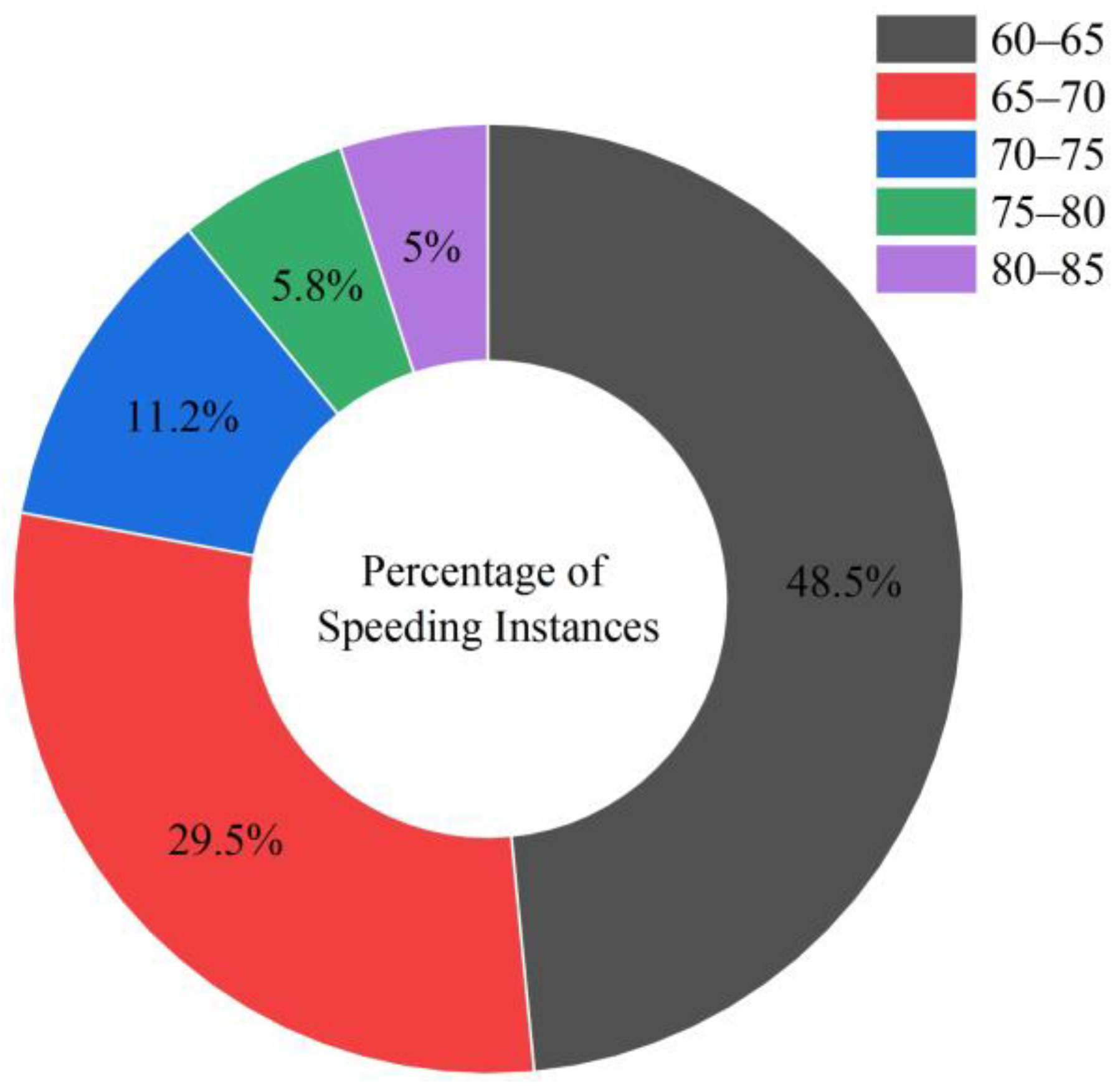
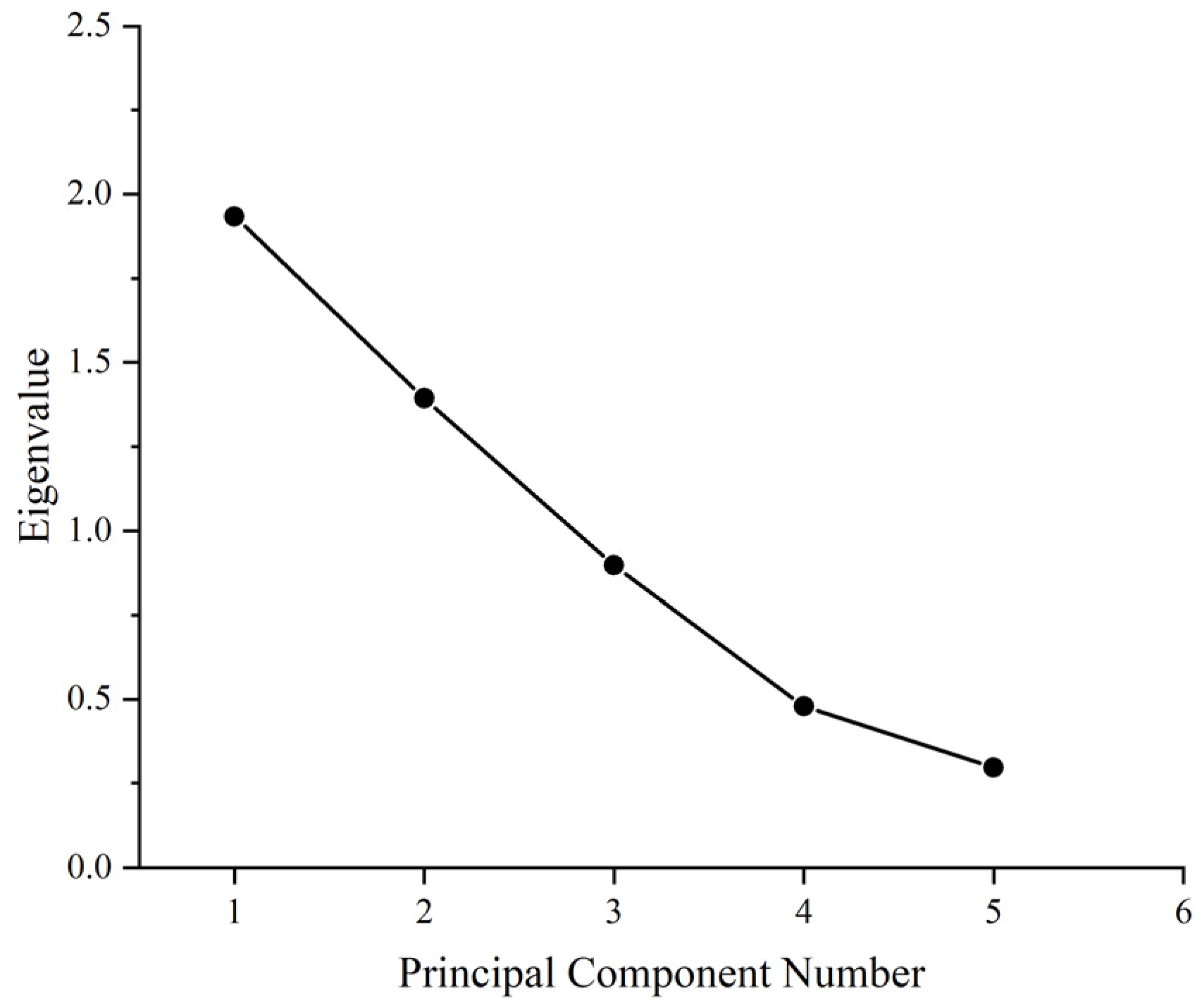
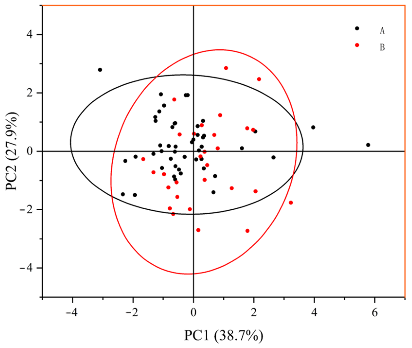
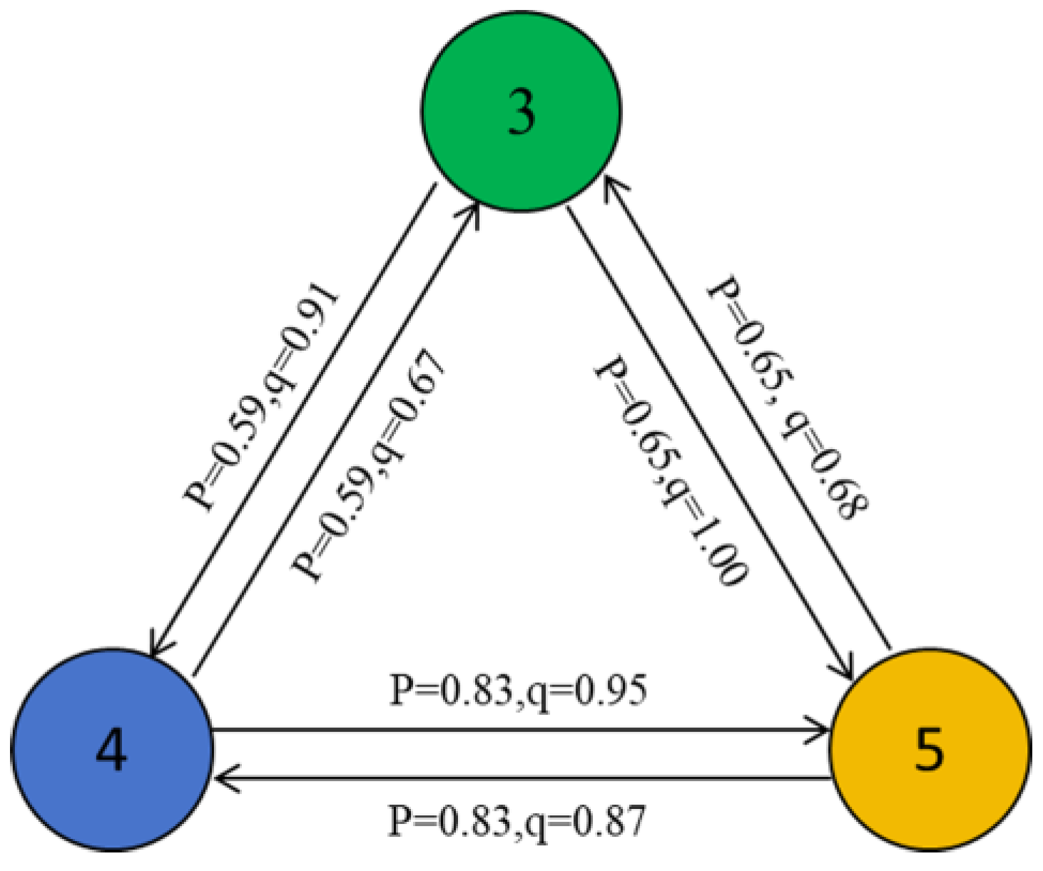
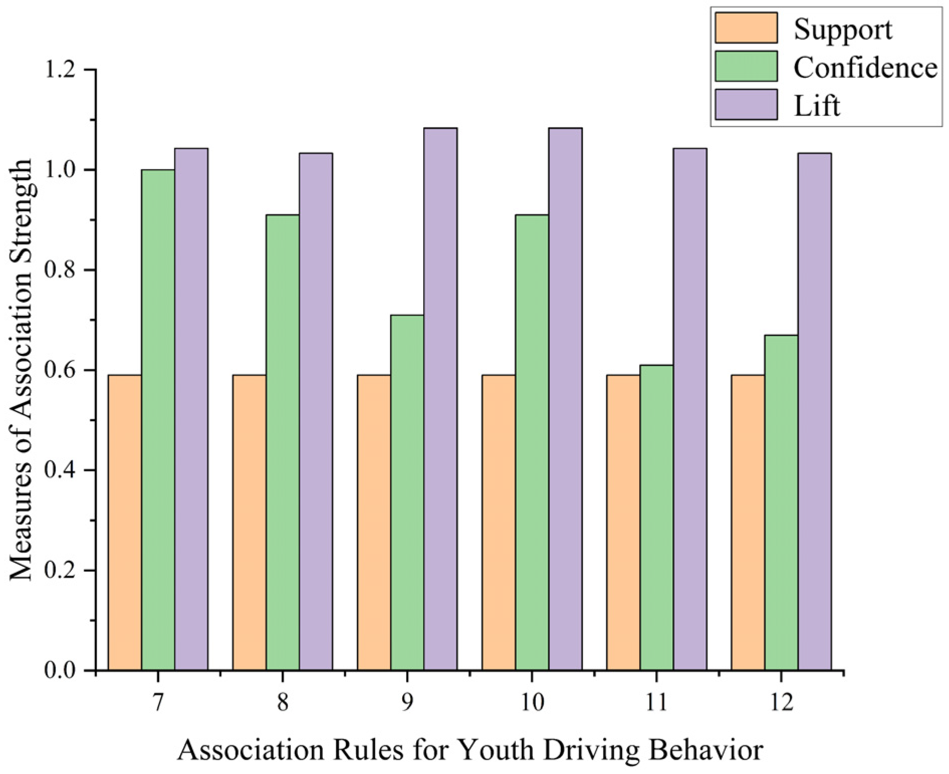
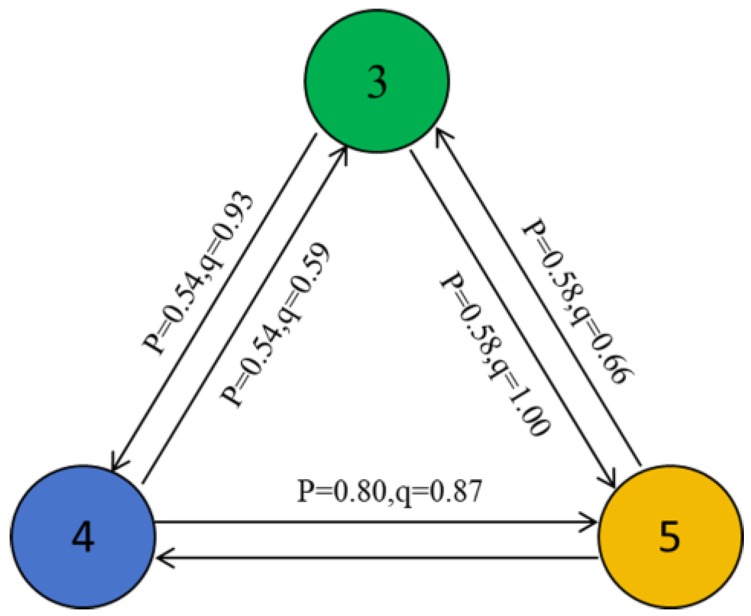
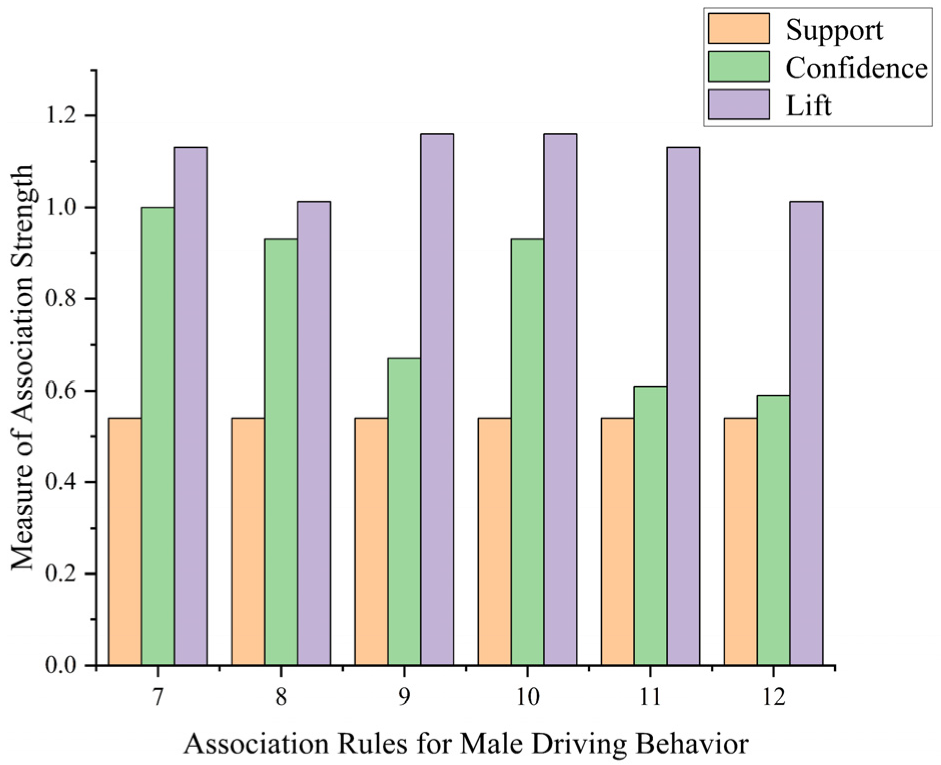
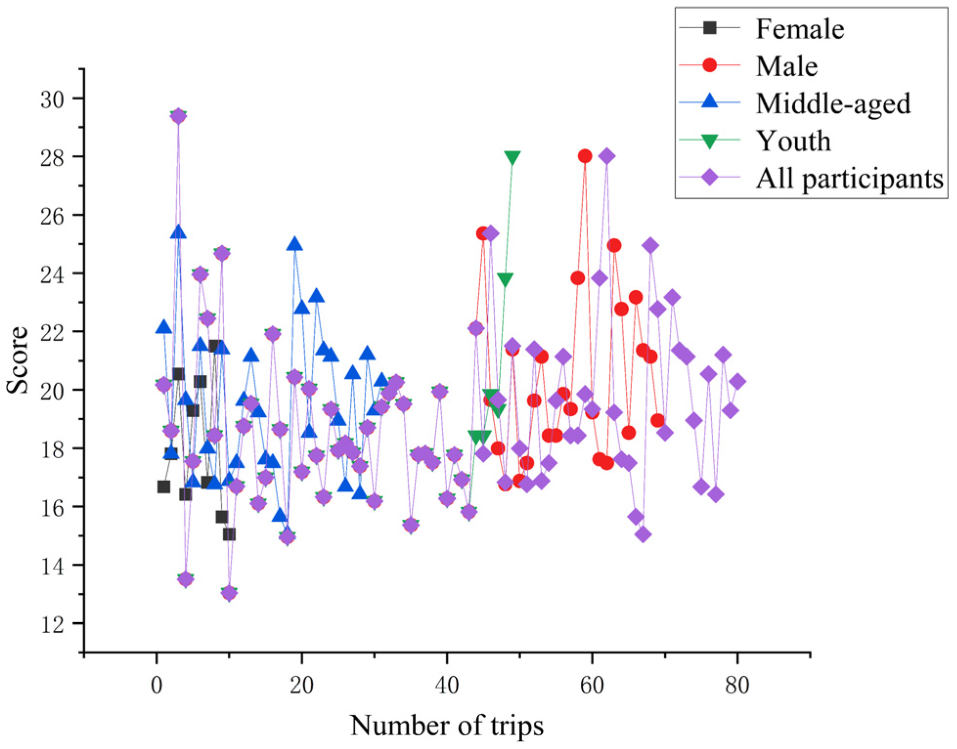
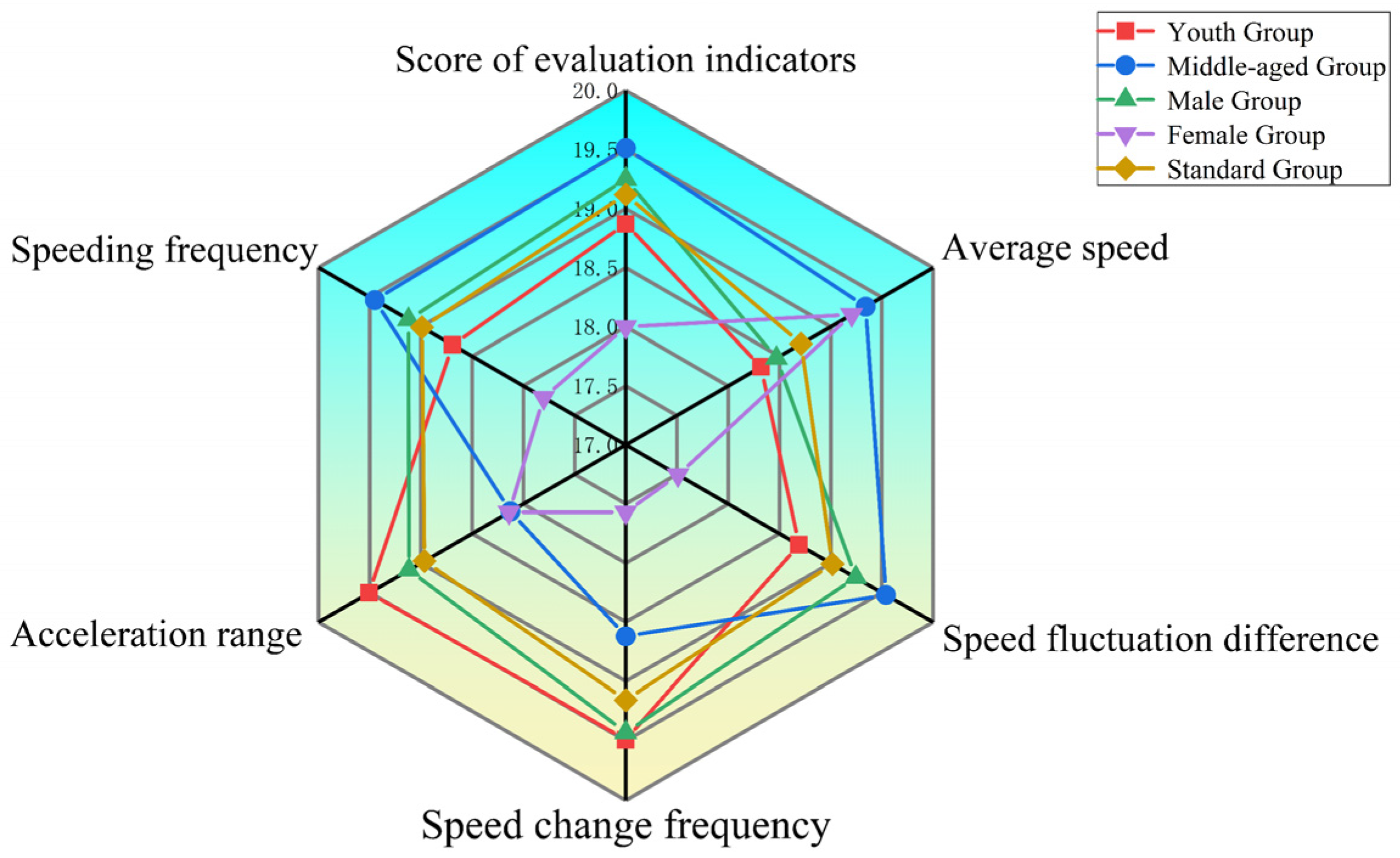
This study collected authentic and comprehensive data on urban high-frequency driving behavior through real-world experiments. Five safety evaluation indicators for driving behavior, along with their thresholds, were chosen. The FP-growth association rule method is employed to model driving behavior and explore the interactions between different unsafe driving behaviors. The findings revealed that unsafe driving behaviors do not occur independently within a single trip; rather, multiple unsafe tendencies may co-occur in terms of the selected aggregated indicators, collectively affecting the driver’s safety. Based on the proposed evaluation method, unsafe driving behaviors were quantitatively assessed, with higher scores indicating greater risk. Safety scores were computed for drivers of different age and gender groups, followed by targeted analysis. Results showed that male drivers and younger drivers exhibited greater score variability than female and middle-aged drivers, suggesting notable differences in driving behavior characteristics. Speeding behavior was found to have the most significant impact on overall safety scores.

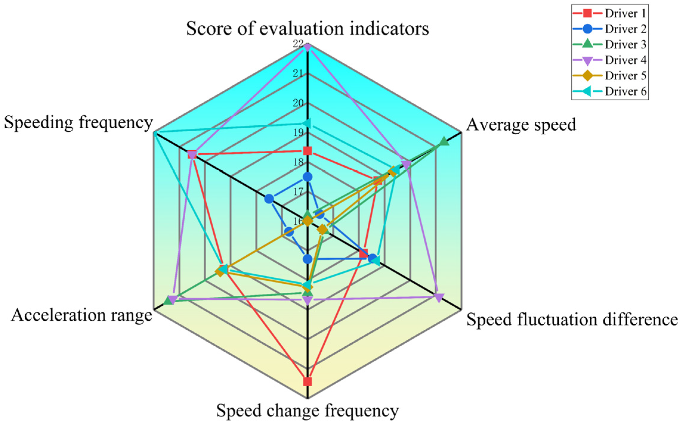
Further analysis of six representative drivers showed that middle-aged drivers changed speed more frequently but with lower fluctuation amplitude, indicating better control likely due to driving experience. Gender differences were also observed in accelerator pedal usage, validating the method’s ability to reflect behavioral traits. The proposed FP-growth-based safety evaluation method can be integrated into driver behavior monitoring systems to generate personalized reports. By translating behavioral data into intuitive safety scores, the method offers actionable feedback to help drivers recognize risks and improve their driving habits. This approach is particularly useful for fleet management companies, as it enables the evaluation of each driver’s safety performance based on aggregated trip-level indicators. By continuously monitoring the safety scores across multiple trips, managers can identify drivers with potentially unsafe behavior patterns and provide targeted feedback or training interventions. In this way, it contributes to reducing traffic risk and improving overall fleet safety management. Additionally, the method can support autonomous driving systems by improving behavior prediction and safety response strategies, thereby enhancing road safety performance. Furthermore, analyzing behavioral characteristics across driver groups (e.g., by age or gender) can assist traffic authorities in identifying high-risk populations, developing targeted safety policies, and optimizing traffic signal control and road design to improve urban traffic safety.

4.2. Limitations and Future Research

This study has two main limitations. First, due to experimental and urban road constraints, data on lateral driving behaviors (e.g., lane changes) were not collected. Future work will address this by integrating gyroscope sensors and high-definition cameras to capture lateral motion and lane information, enabling analysis of behaviors such as lane changes, overtaking, and turning. Data will also be collected under more diverse conditions, including off-peak hours, expressways, suburban roads, and adverse weather or nighttime environments. Second, the current method focuses on post-trip evaluation and does not support real-time feedback. Future research will explore identifying key safety-related parameters for real-time monitoring and feedback, aiming to proactively enhance driving safety. In addition, personalized feedback strategies will be developed by combining behavior association rules with individual driver characteristics.

References

1. Fan, R.; Li, G.; Wu, Y. State Estimation of Distributed Drive Electric Vehicle Based on Adaptive Kalman Filter. Sustainability 2023, 15, 13446. [Google Scholar] [CrossRef]
2. Miyajima, C.; Takeda, K. Driver-Behavior Modeling Using On-Road Driving Data: A New Application for Behavior Signal Processing. IEEE Signal Process. Mag. 2016, 33, 14–21. [Google Scholar] [CrossRef]
3. Xu, Y.; Pradhan, A.K. Modeling Drivers’ Reaction When Being Tailgated: A Random Forests Method. J. Saf. Res. 2021, 78, 28–35. [Google Scholar] [CrossRef]
4. Gitelman, V.; Doveh, E. Examining the Safety Impacts of High-Occupancy Vehicle Lanes: International Experience and an Evaluation of First Operation in Israel. Sustainability 2023, 15, 13976. [Google Scholar] [CrossRef]
5. He, Y.; Gong, X.; Yuan, C.; Shen, J.; Du, Y. Lateral Obstacle Avoidance Control Based on Driving Behavior Recognition of the Preceding Vehicles in Adjacent Lanes. Automatisierungstechnik 2020, 68, 880–892. [Google Scholar] [CrossRef]
6. Wang, J.; Pan, C.; Li, Z. Coordinated Adaptive Cruise Control with Integration of Driving Behaviors Based on Prediction for Surrounding Vehicles Status. Proc. Inst. Mech. Eng. Part J. Automob. Eng. 2023, 239, 1384–1405. [Google Scholar] [CrossRef]
7. Tawfeek, M.H.; El-Basyouny, K. A context identification layer to the reasoning subsystem of context-aware driver assistance systems based on proximity to intersections. Transp. Res. Part C Emerg. Technol. 2020, 117, 102703. [Google Scholar] [CrossRef]
8. Tawfeek, M.H.; El-Basyouny, K. Location-Based Analysis of Car-Following Behavior during Braking Using Naturalistic Driving Data. Can. J. Civ. Eng. 2020, 47, 498–505. [Google Scholar] [CrossRef]
9. Ferreira, J.; Carvalho, E.; Ferreira, B.V.; De Souza, C.; Suhara, Y.; Pentland, A.; Pessin, G. Driver Behavior Profiling: An Investigation with Different Smartphone Sensors and Machine Learning. PLoS ONE 2017, 12, e0174959. [Google Scholar] [CrossRef]
10. Zhao, C.; Li, L.; Pei, X.; Li, Z.; Wang, F.-Y.; Wu, X. A Comparative Study of State-of-the-Art Driving Strategies for Autonomous Vehicles. Accid. Anal. Prev. 2021, 150, 105937. [Google Scholar] [CrossRef]
11. Zhu, X.; Yuan, Y.; Hu, X.; Chiu, Y.-C.; Ma, Y.-L. A Bayesian Network Model for Contextual versus Non-Contextual Driving Behavior Assessment. Transp. Res. Part C Emerg. Technol. 2017, 81, 172–187. [Google Scholar] [CrossRef]
12. Toledo, T.; Musicant, O.; Lotan, T. In-Vehicle Data Recorders for Monitoring and Feedback on Drivers’ Behavior. Transp. Res. Part C Emerg. Technol. 2008, 16, 320–331. [Google Scholar] [CrossRef]
13. Qu, Y.; Li, Z.; Liu, Q.; Pan, M.; Zhang, Z. Crash/Near-Crash Analysis of Naturalistic Driving Data Using Association Rule Mining. J. Adv. Transp. 2022, 2022, 6562649. [Google Scholar] [CrossRef]
14. Kong, X. Understanding Speeding Behavior from Naturalistic Driving Data_ Applying Classification Based Association Rule Mining. Accid. Anal. Prev. 2020, 144, 105620. [Google Scholar] [CrossRef]
15. Sun, M. Analysis of HAZMAT Truck Driver Fatigue and Distracted Driving with Warning-Based Data and Association Rules Mining. J. Traffic Transp. Eng. (Engl. Ed.) 2023, 10, 132–142. [Google Scholar] [CrossRef]
16. Das, A.; Ahmed, M.M.; Ghasemzadeh, A. Using Trajectory-Level SHRP2 Naturalistic Driving Data for Investigating Driver Lane-Keeping Ability in Fog: An Association Rules Mining Approach. Accid. Anal. Prev. 2019, 129, 250–262. [Google Scholar] [CrossRef]
17. Ding, Y.; Zhao, X.; Wu, Y.; He, C.; Liu, S.; Tian, R. Optimization Method to Reduce the Risky Driving Behaviors of Ride-Hailing Drivers. J. Safety Res. 2023, 85, 442–456. [Google Scholar] [CrossRef]
18. Hussain, B.; Miwa, T.; Sato, H.; Morikawa, T. Subjective Evaluations of Self and Others’ Driving Behaviors: A Comparative Study Involving Data from Drivers in Japan, China, and Vietnam. J. Safety Res. 2023, 84, 316–329. [Google Scholar] [CrossRef]
19. Faria, M.V.; Duarte, G.O.; Varella, R.A.; Farias, T.L.; Baptista, P.C. Driving for Decarbonization: Assessing the Energy, Environmental, and Economic Benefits of Less Aggressive Driving in Lisbon, Portugal. Energy Res. Soc. Sci. 2019, 47, 113–127. [Google Scholar] [CrossRef]
20. Kinnear, N. An Experimental Study of Factors Associated with Driver Frustration and Overtaking Intentions. Accid. Anal. Prev. 2015, 79, 221–230. [Google Scholar] [CrossRef]
21. Eusofe, Z.; Evdorides, H. Assessment of Road Safety Management at Institutional Level in Malaysia: A Case Study. IATSS Res. 2017, 41, 172–181. [Google Scholar] [CrossRef]
22. Zhou, T.; Zhang, J. Analysis of Commercial Truck Drivers’ Potentially Dangerous Driving Behaviors Based on 11-Month Digital Tachograph Data and Multilevel Modeling Approach. Accid. Anal. Prev. 2019, 132, 105256. [Google Scholar] [CrossRef] [PubMed]
23. Chong, L.; Abbas, M.M.; Medina Flintsch, A.; Higgs, B. A Rule-Based Neural Network Approach to Model Driver Naturalistic Behavior in Traffic. Transp. Res. Part C Emerg. Technol. 2013, 32, 207–223. [Google Scholar] [CrossRef]
24. Chen, J.; Ning, X.; Li, Y.; Yang, G.; Wu, P.; Chen, S. A Fuzzy Control Strategy for the Forward Speed of a Combine Harvester Based on KDD. Appl. Eng. Agric. 2017, 33, 15–22. [Google Scholar] [CrossRef]
25. Yu, B.; Chen, Y.; LeBlanc, D.J. Effects of an Integrated Collision Warning System on Risk Compensation Behavior: An Examination under Naturalistic Driving Conditions. Accid. Anal. Prev. 2021, 163, 106450. [Google Scholar] [CrossRef]
26. Zhao, Y.; Liang, J.; Chen, L.; Wang, Y.; Gong, J. Evaluation and Prediction of Free Driving Behavior Type Based on Fuzzy Comprehensive Support Vector Machine. J. Intell. Fuzzy Syst. 2022, 42, 2863–2879. [Google Scholar] [CrossRef]
27. Zhang, Y. Environmental Screening Model of Driving Behavior for an Electric Bus Entering and Leaving Stops. Transp. Res. Part D Transp. Environ. 2022, 112, 103464. [Google Scholar] [CrossRef]
28. Wang, J. Driving Risk Assessment Using Near-Crash Database through Data Mining of Tree-Based Model. Accid. Anal. Prev. 2015, 84, 54–64. [Google Scholar] [CrossRef]
29. Paefgen, J.; Staake, T.; Fleisch, E. Multivariate Exposure Modeling of Accident Risk: Insights from Pay-as-You-Drive Insurance Data. Transp. Res. Part A Policy Pract. 2014, 61, 27–40. [Google Scholar] [CrossRef]
30. Raza, A.; Saber, K.; Hu, Y.; Ray, R.L.; Kaya, Y.Z.; Dehghanisanij, H.; Kisi, O.; Elbeltagi, A. Modelling Reference Evapotranspiration Using Principal Component Analysis and Machine Learning Methods under Different Climatic Environments. Irrig. Drain. 2023, 72, 945–970. [Google Scholar] [CrossRef]
31. Wang, H.; Gu, J.; Wang, M. A Review on the Application of Computer Vision and Machine Learning in the Tea Industry. Front. Sustain. Food Syst. 2023, 7, 1172543. [Google Scholar] [CrossRef]
32. Liang, Y.; Lin, H.; Kang, W.; Shao, X.; Cai, J.; Li, H.; Chen, Q. Application of Colorimetric Sensor Array Coupled with Machine-learning Approaches for the Discrimination of Grains Based on Freshness. J. Sci. Food Agric. 2023, 103, 6790–6799. [Google Scholar] [CrossRef] [PubMed]
33. Mohammed, M.; Ke, Y.; Gao, J.; Zhang, H.; El-Basyouny, K.; Qiu, T.Z. Connected Vehicle V2I Communication Application to Enhance Driver Awareness at Signalized Intersections. In Proceedings of the CSCE Resilient Infrastructure Conference, London, ON, Canada, 1–4 June 2016. [Google Scholar]
34. Jun, J.; Guensler, R.; Ogle, J. Differences in Observed Speed Patterns between Crash-Involved and Crash-Not-Involved Drivers: Application of in-Vehicle Monitoring Technology. Transp. Res. Part C Emerg. Technol. 2011, 19, 569–578. [Google Scholar] [CrossRef]
35. Pierson, A.; Schwarting, W.; Karaman, S.; Rus, D. Learning Risk Level Set Parameters from Data Sets for Safer Driving. In Proceedings of the 2019 IEEE Intelligent Vehicles Symposium (IV), Paris, France, 9–12 June 2019; IEEE: Paris, France, 2019; pp. 273–280. [Google Scholar]
36. Han, J.; Pei, J.; Yin, Y. Mining Frequent Patterns without Candidate Generation. ACM SIGMOD Rec. 2000, 29, 1–12. [Google Scholar] [CrossRef]
37. Eboli, L.; Mazzulla, G.; Pungillo, G. Combining Speed and Acceleration to Define Car Users’ Safe or Unsafe Driving Behaviour. Transp. Res. Part C Emerg. Technol. 2016, 68, 113–125. [Google Scholar] [CrossRef]
38. He, S.; Wang, Y.; Chen, Y.; Xiao, F.; Deng, J.; Xu, E. Research on Safety Evaluation of Commercial Vehicle Driving Behavior Based on Data Mining Technology. J. Sens. 2021, 2021, 9927348. [Google Scholar] [CrossRef]
39. Ji, S.; Zhang, K.; Tian, G.; Yu, Z.; Lan, X.; Su, S.; Cheng, Y. Evaluation Method of Naturalistic Driving Behaviour for Shared-Electrical Car. Energies 2022, 15, 4625. [Google Scholar] [CrossRef]
40. Jin, L.; Guo, B.; Jiang, Y.; Wang, F.; Xie, X.; Gao, M. Study on the Impact Degrees of Several Driving Behaviors When Driving While Performing Secondary Tasks. IEEE Access 2018, 6, 65772–65782. [Google Scholar] [CrossRef]
41. Rahman, M.S.; Abdel-Aty, M. Longitudinal Safety Evaluation of Connected Vehicles’ Platooning on Expressways. Accid. Anal. Prev. 2018, 117, 381–391. [Google Scholar] [CrossRef]
42. Kim, S.-W.; Eom, J.-O. Ship Carbon Intensity Indicator Assessment via Just-in-Time Arrival Algorithm Based on Real-Time Data: Case Study of Pusan New International Port. Sustainability 2023, 15, 13875. [Google Scholar] [CrossRef]
43. Changizian, S.; Ahmadi, P.; Raeesi, M.; Javani, N. Performance Optimization of Hybrid Hydrogen Fuel Cell-Electric Vehicles in Real Driving Cycles. Int. J. Hydrogen Energy 2020, 45, 35180–35197. [Google Scholar] [CrossRef]
44. Ma, Y.; Li, W.; Tang, K.; Zhang, Z.; Chen, S. Driving Style Recognition and Comparisons among Driving Tasks Based on Driver Behavior in the Online Car-Hailing Industry. Accid. Anal. Prev. 2021, 154, 106096. [Google Scholar] [CrossRef] [PubMed]
45. Zeng, Y.; Yin, S.; Liu, J.; Zhang, M. Research of Improved FP-Growth Algorithm in Association Rules Mining. Sci. Program. 2015, 2015, 910281. [Google Scholar] [CrossRef]
46. Liu, R.X.; Kuang, J.; Gong, Q.; Hou, X.L. Principal Component Regression Analysis with Spss. Comput. Methods Programs Biomed. 2003, 71, 141–147. [Google Scholar] [CrossRef]
Figure 1. Experimental route and experimental car: (a) Experiment route in urban Zhenjiang; (b) Electric vehicle used for data collection.
Sustainability 17 04067 g001
Figure 2. Signal acquisition and positioning devices used in the vehicle experiment: (a) Electric vehicle, Chery ARRIZO; (b) CANOE vehicle-mounted signal acquisition device; (c) Radar inertial navigation equipment (XW-SC3663).
Sustainability 17 04067 g002
Figure 3. Actual urban road segment selected for high-frequency data collection.
Sustainability 17 04067 g003
Figure 4. Sample of raw signal data collected via CANOE onboard system.
Sustainability 17 04067 g004
Figure 5. Workflow of high-frequency driving data preprocessing and feature extraction.
Sustainability 17 04067 g005
Figure 6. Distribution of average speed across all experimental urban trips.
Sustainability 17 04067 g006
Figure 7. Boxplot of average speed during peak hours in urban road segments.
Sustainability 17 04067 g007
Figure 8. Distribution of acceleration-deceleration ranges across all trips.
Sustainability 17 04067 g008
Figure 9. Distribution of vehicle speeding frequency on urban roads.
Sustainability 17 04067 g009
Figure 10. Processing logic of the FP-growth algorithm applied to driving behavior indicators.
Sustainability 17 04067 g010
Figure 11. Scree plot of principal component analysis for evaluation indicators.
Sustainability 17 04067 g011
Figure 12. Score plot of principal component analysis showing indicator relationships.
Sustainability 17 04067 g012
Figure 13. Visualization of association strength among driving behavior indicators.
Sustainability 17 04067 g013
Figure 14. Pairwise association strength between indicators in the young driver group.
Sustainability 17 04067 g014
Figure 15. Association rules among three evaluation indicators for young driver group.
Sustainability 17 04067 g015
Figure 16. Association rules between two evaluation indicators for male driver group.
Sustainability 17 04067 g016
Figure 17. Association rules between three evaluation indicators for male driver group.
Sustainability 17 04067 g017
Figure 18. Comparative safety scores across driver types under urban peak traffic.
Sustainability 17 04067 g018
Figure 19. Radar chart of key behavior indicators among different driver groups.
Sustainability 17 04067 g019
Figure 20. Distribution of accelerator pedal travel for six selected drivers.
Sustainability 17 04067 g020
Figure 21. Radar comparison of five behavior indicators for six selected drivers.
Sustainability 17 04067 g021