A Variable Neighborhood Search Algorithm for the Integrated Berth Allocation and Quay Crane Assignment Problem

Abstract

To improve the utilization of port resources and reduce the consumption of resources due to vessel waiting and delays, this paper investigates the Berth Allocation and Quay Crane Assignment Problem (BACAP) in container ports, focusing on the Quay Crane (QC) profile. The objective is to assign berths, berthing times, and QC profiles to vessels arriving at the port within a given planning horizon, thereby extending the traditional BACAP framework. To minimize the sum of idle time costs caused by vessel waiting and delay time costs due to late vessel departures, a mixed-integer linear programming (MILP) model is proposed. Additionally, a variable neighborhood search (VNS) algorithm is designed to solve the model, tailored to the specific characteristics of the problem. The proposed MILP model and VNS algorithm are evaluated using two sets of BACAP instances. The numerical results demonstrate the effectiveness of both the model and the algorithm, showing that VNS efficiently and reliably solves instances of various sizes. Furthermore, each neighborhood structure contributes uniquely to the iterative process. This study also analyzes the impact of different idle and delay costs on BACAP, providing valuable managerial insights. The proposed framework contributes to enhancing operational efficiency and supports sustainable port management.

1. Introduction

In the context of the rapid development of intelligent transportation systems, coupled with the ongoing advancement of global economic integration and the expansion of international trade, ports—critical hubs for cargo transportation—are playing an increasingly prominent role within the broader intelligent transportation ecosystem. The increasing prevalence of large-scale vessels has significantly heightened the operational pressure on ports, presenting considerable challenges to both their operational efficiency and service quality during the process of digital transformation. One of the key strategies for effectively managing port operations is the optimization of berth and QC schedules, as these are among the most essential yet limited resources within the port system. From a sustainability perspective, inefficient utilization of core port resources results in prolonged vessel idle time, excessive energy consumption, and exacerbated greenhouse gas emissions—factors that collectively compromise both the environmental and economic sustainability of port operations. Consequently, the development of intelligent and adaptive scheduling frameworks is essential not only for enhancing operational efficiency but also for minimizing environmental impact and advancing green transformation of seaports.

Moreover, seaport operations should not be viewed in isolation. As highlighted in recent research [1], maritime transport forms an integral part of intermodal logistics systems, where seamless coordination with inland transport modes—such as rail and road—is essential. Optimizing berth and quay crane scheduling at ports not only improves port-side efficiency but also facilitates smoother cargo transfers across the entire supply chain, ultimately benefiting manufacturers, distributors, sellers, and customers.

In the Berth Allocation and Quay Crane Assignment Problem, QC assignment can be categorized into two types: time-invariant QC assignment and time-variant QC assignment. Time-invariant QC assignment refers to a scenario in which a fixed number of QCs serve a vessel throughout its entire operational process. The BACAP, considering time-invariant QC assignment, has received significant attention in the literature. Imai et al. [2] introduced a formulation for BACAP with time-invariant QC assignment and proposed two novel models: a 0–1 integer linear programming (ILP) model for the BACAP and a mixed-integer linear programming (MILP) model. Building on the model developed by Meisel and Bierwirth [3], Iris et al. [4] introduced a generalized set partitioning approach to address the BACAP, which incorporates two QC assignment strategies. Wang et al. [5] investigated the time-invariant Berth Allocation and Quay Crane Assignment Scheduling Problem (BACASP) within the context of carbon emission tax policies, incorporating both single and segmented tax rates. They developed an optimization model and proposed several equivalent or relaxed models to enhance computational efficiency. Wang, Miao et al. [6] introduced a two-stage robust optimization model for time-invariant BACAP under uncertain conditions, achieving a comprehensive solution with enhanced robustness. Sharifi et al. [7] developed an integrated BACAP model with time-invariant QC assignment, considering vessel emission and speed optimization. Cheimanoff et al. [8] proposed a new MILP model to solve the time-invariant BACAP, considering continuous terminal topology and dynamic ship arrivals. Correcher et al. [9] proposed a novel MILP model for the continuous BACAP and demonstrated its capability to solve instances involving up to 50 vessels. Ji et al. [10] investigated time-invariant BACAPs under stochastic vessel arrivals and formulated a MILP model, aimed at minimizing the total port time of vessels. They employed a Multi-Objective Constrained Handling (MOCH) strategy and proposed an Enhanced Non-dominated Sorting Genetic Algorithm II (ENSGA-II) to solve the problem. Bouzekri et al. [11] addressed the integrated problem of the Laycan Allocation Problem, the dynamic continuous Berth Allocation Problem (BAP), and the time-invariant QC Assignment Problem in tidal ports. Xiang et al. [12] redefined the discrete berth allocation and time-invariant QC assignment problem as a constraint-limited resource scheduling problem. Then, a branch-and-cut algorithm was proposed to solve the redefined problem efficiently. Ji et al. [13] studied a dynamic Berth Allocation and time-invariant QC Assignment specific problem when unscheduled vessels arrive at the port (UBACASP), considering factors such as dynamic vessel arrivals and non-crossing constraints between quay cranes. Building upon their previous research [14], Song et al. [15] integrated time-invariant QC Assignment into the Multi-port Berth Allocation Problem (MBACAP) for the first time, constructing a MILP model. In comparison to previous studies on the Multi-port Berth Allocation Problem (MBAP), this model considers the impact of specific QC assignments on vessel handling time and incorporates additional constraints to reflect a more realistic scheduling scenario.

While time-invariant QC assignment reduces the computational complexity of the model, it also limits the practical applicability of the solution. In contrast, time-variant QC assignment not only maximizes QC utilization but also more accurately reflects real-world operations. This approach offers greater flexibility by allowing the number of QCs allocated to a vessel to change throughout its operational period. As a result, numerous studies have been conducted on time-variant QC assignment.

Park and Kim [16] developed a MILP model to schedule both berths and QCs. Meisel and Bierwirth [3] critiqued Park and Kim’s linear relationship between vessel handling time and the number of QCs, proposing an alternative model that accounts for interference between QCs and the deviation from the optimal berthing position, which influences handling time. Raa et al. [17] introduced a MILP model that considers vessel priorities, berthing preferences, and handling times influenced by container volume and quay crane availability. This model was solved using a hybrid heuristic and validated with real-world data. Li et al. [18] extended the BACAP by incorporating quay crane coverage constraints, formulating a nonlinear mixed-integer programming model based on continuous berth and quay crane coverage constraints. Wang, Hu et al. [19] incorporated onshore power supply (OPS) allocation into time-variant BACAP to support carbon emission reduction policies. Guo et al. [20] integrated time-variant BACAP with Yard Allocation Problem (YAP) and formulated a mixed-integer nonlinear programming (MINLP) model. Xiang and Liu [21] developed an almost robust model for time-variant BACAP, considering uncertainties in the late arrival of ships and inflation of container quantity. They also proposed a decomposition method to solve this complex problem. Li et al. [22] proposed a bi-objective optimization model for BACAP, aiming to minimize both the total vessel turnaround time and the penalty costs associated with quay crane maintenance earliness and tardiness. Xu et al. [23] developed a comprehensive mathematical model for the C/T-V (Continuous and Time-variant) BACAP and proposed a memetic algorithm with a heuristic decoding strategy, capable of efficiently solving large-scale instances involving up to 60 vessels. Zou et al. [24] developed a swarm optimization algorithm with intra- and inter-hierarchical competition (I2HCSO) for solving large-scale BACAP. Ran et al. [25] incorporated quay crane movement energy consumption for the first time, where a MILP model was formulated to minimize the maximum completion time of all vessels and total energy consumption. Thanos et al. [26] addressed QC working range constraints and developed a model to minimize container trans-shipment distances within the terminal yard. They proposed a heuristic algorithm based on fast local search to solve the BACAP. Malekahmadi et al. [27] considered safe distances between quay cranes and non-crossing constraints. They formulated an integer programming model for the integrated continuous berth allocation, time-variant QC assignment, and QC scheduling problem.

However, within the planning horizon, frequent quay crane exchanges are not always optimal, as they incur time and cost penalties. As a result, several studies have imposed constraints on QC exchanges to mitigate these drawbacks. Zhang et al. [28] argued that frequent changes in QC allocation led to substantial relocation costs. To address this, they introduced limitations on the number of QC changes during vessel service, taking into account the length of each QC and the berthing range it can serve. Türkoğulları et al. [29] integrated QC relocation costs into their model, incorporating both fixed and distance-dependent variable costs. In a subsequent study [30], the same team strengthened the constraints on QC changes, stipulating that once a QC is assigned to a vessel, it can only be reassigned upon the completion of the vessel’s loading/unloading operations.

Giallombardo et al. [31] introduced the definition of QC profiles to effectively balance quay crane utilization and the frequency of QC exchanges. Each QC profile contains information on the number of work shifts and the number of QCs assigned to each work shift. The QC profile transforms the time-invariant QC assignment into a time-variant assignment by varying the number of QCs between work shifts, thus improving QC utilization and aligning the model more closely with real-world operations. By limiting the difference in the number of QCs between shifts to no more than two, the non-crossing constraint between QCs can be addressed. Additionally, by restricting QCs to move only between shifts, the number of QC exchanges during a vessel’s service can be controlled. Vacca et al. [32] explored the time-variant BACAP in seaport container terminals, building upon the BAP defined by Giallombardo et al. [31], and introduced a column generation (CG) algorithm to solve the problem. Xie et al. [33] further developed the BACAP based on QC profiles, aiming at minimizing berth and time deviations. This problem was solved using a branch-and-price algorithm within the Dantzig–Wolfe decomposition framework. Tang et al. [34] were the first to incorporate QC efficiency uncertainty into the BACAP with QC profiles, considering tidal time windows. They formulated a MILP model to minimize the total cost of vessel delay in berthing and departure, solving it using a column generation algorithm. Xiang et al. [35] investigated automated trans-shipment hubs and introduced a multi-objective optimization model that simultaneously addresses berth allocation, quay crane assignment, and yard allocation by incorporating QC profiles. They proposed an efficient adaptive dynamic scheduling strategy to balance the trade-offs among multiple objectives adaptively.

To summarize, existing studies have made significant progress in modeling the BACAP under both time-invariant and time-variant quay crane assignments. However, most models are constrained by computational scalability and heavily rely on exact solution methods. Heuristic methods for BACAP incorporating QC profiles, particularly for large-scale instances, remain underexplored. Moreover, the BACAP has been proven to be NP-hard [16], and as the scale of the problem rises, these exact algorithms face significant challenges related to excessive computation time and memory consumption. To address these challenges, this paper proposes an effective VNS algorithm to solve the proposed MILP model of the BACAP. The effectiveness and superiority of the VNS algorithm are demonstrated through a comparative analysis with other algorithms. The results of this research provide theoretical support and practical guidance for port operation management, offering significant theoretical and practical value.

The BACAP exhibits typical characteristics of multi-resource allocation, multi-task scheduling, and time window constraints. It shares significant similarities with the flexible job shop scheduling problem (FJSP) and the Vehicle Routing Problem with Time Windows (VRPTW). For the FJSP, Yang et al. [36] addressed distributed heterogeneous assembly flexible job shop scheduling problems and proposed a Q-learning-based improved multi-objective genetic algorithm. Zhang et al. [37] formulated a MILP model for the dual-resource flexible job shop scheduling problem in production line reconfiguration scenarios (DRFJSP-PLR) and proposed a rule-guided exemplar learning genetic algorithm with neighborhood search (RgELGA_NS). Shao et al. [38] developed a multi-objective optimal scheduling method for variable sublot flexible shops, incorporating switching time and operator constraints, and proposed an adaptive job scheduling NSGA-II (AJS-NSGAII) algorithm. For the VRPTW, Liu et al. [39] proposed an improved genetic algorithm based on clustering methods and the longest common substring (LCS) between elite and inferior individuals. Su et al. [40] introduced a lightweight genetic algorithm with variable neighborhood search (LGAVNS), combining GA as the upper-level algorithm and VNS as the local search method, to solve a multi-depot green VRPTW considering customer satisfaction (MDGVRPTW-CS). In conclusion, heuristic and metaheuristic algorithms have become prominent research topics in complex scheduling problems.

This paper investigates the BACAP within a VNS framework, leveraging its multi-resource collaborative scheduling feature. The design of solution and neighborhood structures in this study provides valuable insights for solving FJSP and VRPTW problems.

The main contributions of this study are as follows:

(1)

A MILP model is formulated for the discrete and time-variant BACAP based on QC profiles, aiming to minimize the costs of vessel waiting and delayed departures while considering berth time windows and spatiotemporal non-overlapping constraints among vessels.

(2)

A VNS algorithm is developed for the BACAP with QC profiles, in which a tailored solution structure is designed, and multiple neighborhood structures are incorporated to enhance the search efficiency and effectiveness. The algorithm can calculate instances of 40 ships.

(3)

The effectiveness of the proposed model and algorithm is validated through two sets of computational experiments, and sensitivity analysis on the weights of waiting and delay costs provides valuable managerial insights for port operations.

The remainder of this paper is organized as follows: Section 2 presents the problem statement, Section 3 formulates the MILP model for the BACAP, Section 4 elaborates on the VNS algorithm designed according to the characteristics of the BACAP, and Section 5 provides the numerical experiments that include two sets of instances. Section 6 presents the conclusion.

2. Problem Statement

Prior to the arrival of vessels, relevant information—such as the vessel type, estimated time of arrival (ETA), estimated time of departure (ETD), and the number of containers to be handled—is collected by the port of call. The port then assigns berths, berthing time steps, and a reliable QC profile to vessels arriving within a given planning horizon. The QC profile, introduced by Giallombardo et al. [31], represents a combination of time duration and the assigned number of QCs at each time step. This definition is based on the end-of-shift assumption, which means that QCs can be moved during a vessel’s service, but they cannot be reassigned until the end of a work shift.

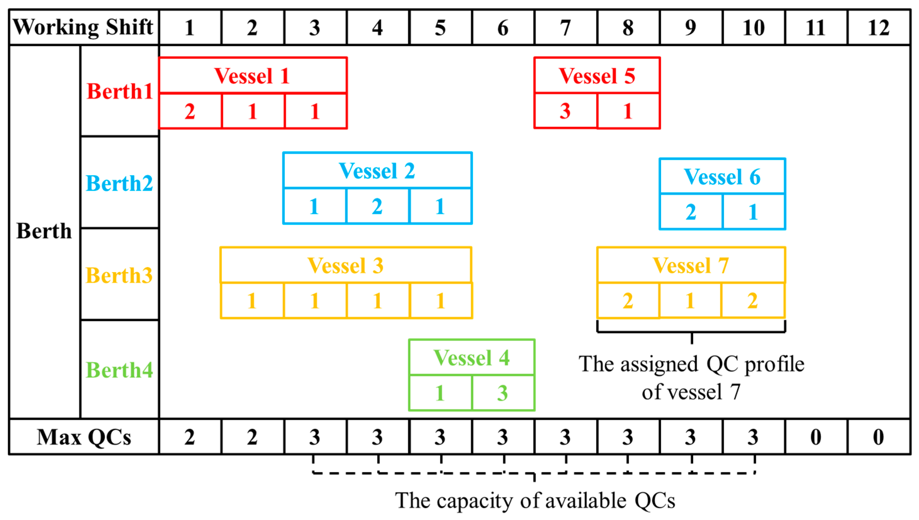
The handling time for each vessel is determined precisely by the assigned QC profile, rather than by a predefined constant. For further details on the QC profile definition, readers are referred to Giallombardo et al. [31]. The port can assign a QC profile to determine the number of QCs allocated to a specific vessel at each time step during the vessel’s service. To better understand the BACAP and the QC profile, a berthing plan for five vessels at three berths over 12 work shifts is illustrated in Figure 1. In this figure, one work shift is equivalent to one step. In the figure, vessel 1 begins berthing in work shift 1, berths for three work shifts, and departs in work shift 3. Based on the assigned QC profile, the number of QCs servicing the vessel in each time step is known. For vessel 1, two QCs are allocated in work shift 1, and one QC is allocated in both work shifts 2 and 3.

In this paper, a MILP model for the BACAP is developed for discrete berths, considering the non-overlapping constraints of vessels, the available time windows for ships and berths, and the constraints associated with the QC profile.

The objective is to minimize the total cost of delayed berthing and the total cost of delayed departures. In the existing literature on the BACAP, various objectives have been explored to reflect different operational priorities. For instance, Wang et al. [41] developed a model for minimizing the total terminal scheduling cost, which includes berth deviation cost, delayed start delay cost, and delayed departure cost. Li et al. [42] extended the total terminal scheduling cost proposed by Wang et al. [41] by further incorporating the loading and unloading costs of vessels. These objective functions capture diverse optimization goals in port operations. In this study, we focus on two critical and practical objectives:

(1)

Minimizing the delayed berthing time, which captures the cost associated with vessels failing to berth at their expected times;

(2)

Minimizing the delayed departure time, which accounts for the penalties incurred when vessels leave the port later than scheduled.

These objectives are highly relevant to real-world port operations. By reducing vessel waiting and departure delays, this objective contributes to lowering fuel consumption, mitigating greenhouse gas emissions, and improving the overall sustainability of port operations.

The formulation is based on the following assumptions:

(1)

The estimated time of vessel arrival (ETA) and the estimated time of vessel departure (ETD) are discrete and known.

(2)

The container quantity to be handled for each vessel is known.

(3)

The set of available QC profiles for each vessel is known.

(4)

Vessels can only be berthed after their arrival.

(5)

QCs operate on rails and cannot pass each other.

(6)

The number of QCs allocated to a vessel can only be changed between shifts.

3. Model Formulation

This section presents a MILP model for the BACAP, developed based on the approach proposed by Xie et al. [33]. Unlike the model by Xie et al. [33], our model does not consider the effect of the preferred berth of vessels. The objective is to minimize the sum of idle costs caused by vessel waiting and the delay costs from late vessel departures. Additionally, we introduce a linearization constraint related to the objective of minimizing delay costs for late vessel departures.

3.1. Notations

The sets, parameters, and decision variables involved in the proposed MILP model for the BACAP are described in

Table 1. Notations and variables.

Sets and Parameters:
$I$	$\mathrm{Set} \mathrm{of} \mathrm{vessels}, \mathrm{index} \mathrm{by} i$.
$K$	$\mathrm{Set} \mathrm{of} \mathrm{berths}, \mathrm{index} \mathrm{by} k$.
$a_i$	$\mathrm{Estimated} \mathrm{time} \mathrm{step} \mathrm{of} \mathrm{arrival} \mathrm{of} \mathrm{vessel} i\in I$.
$b_i$	$\mathrm{Estimated} \mathrm{time} \mathrm{step} \mathrm{of} \mathrm{departure} \mathrm{of} \mathrm{vessel} i\in I$.
$a_k$	$\mathrm{Start} \mathrm{of} \mathrm{the} \mathrm{available} \mathrm{time} \mathrm{step} \mathrm{of} \mathrm{berth} k\in K$.
$b_k$	$\mathrm{End} \mathrm{of} \mathrm{the} \mathrm{available} \mathrm{time} \mathrm{step} \mathrm{of} \mathrm{berth} k\in K$.
$H$	$\mathrm{Set} \mathrm{of} \mathrm{equal}-\mathrm{length} \mathrm{time} \mathrm{steps}, \mathrm{index} \mathrm{by} h$ $\mathrm{and} t$.
$S$	$\mathrm{Set} \mathrm{of} \mathrm{time}-\mathrm{step} \mathrm{indices} \mathrm{relative} \mathrm{to} \mathrm{a} \mathrm{work} \mathrm{shift}, \mathrm{indexed} \mathrm{by} s$.
$H^s$	$\mathrm{Set} \mathrm{of} \mathrm{all} \mathrm{time} \mathrm{steps} \mathrm{with} \mathrm{the} \mathrm{same} \mathrm{index} s\in S$ $\mathrm{for} \mathrm{all} \mathrm{work} \mathrm{shifts}, \mathrm{index} \mathrm{by} h$ $\mathrm{and} t$.
$Q_i$	$\mathrm{Set} \mathrm{of} \mathrm{feasible} \mathrm{QC} \mathrm{profiles} \mathrm{for} \mathrm{vessels} i\in I$.
$Q_i^s$	$\mathrm{Set} \mathrm{of} \mathrm{feasible} \mathrm{QC} \mathrm{profiles} \mathrm{for} \mathrm{vessels} i\in I$ $\mathrm{for} \mathrm{time} \mathrm{steps} \mathrm{with} \mathrm{index} s\in S$ within a work shift.
$t_i^{sq}$	$\mathrm{Handling} \mathrm{time} \mathrm{of} \mathrm{vessel} i\in I$ $\mathrm{under} \mathrm{QC} \mathrm{profile} q\in Q_i$ $\mathrm{for} \mathrm{time} \mathrm{steps} \mathrm{with} \mathrm{index} s\in S$ within a work shift.
$n_i^{squ}$	$\mathrm{Number} \mathrm{of} \mathrm{QCs} \mathrm{used} \mathrm{by} \mathrm{QC} \mathrm{profiles} q\in Q_i$ $, \mathrm{for} \mathrm{vessel} i\in I$ $, \mathrm{at} \mathrm{time} \mathrm{step} u\in \left\{1,\dots ,t_i^{sq}\right\}$ $\mathrm{if} \mathrm{vessel} i$ $\mathrm{starts} \mathrm{berthing} \mathrm{at} \mathrm{time} \mathrm{steps} \mathrm{with} \mathrm{index} s\in S$ within a work shift.
$Q_h^{max}$	$\mathrm{Max} \mathrm{number} \mathrm{of} \mathrm{QCs} \mathrm{for} \mathrm{time} \mathrm{step} h\in H$.
$M$	A sufficiently large positive value.
$c_i^1$	$\mathrm{Unit} \mathrm{idle} \mathrm{time} \cos \mathrm{t} \mathrm{of} \mathrm{vessel} i\in I$ due to vessel waiting.
$c_i^2$	$\mathrm{Unit} \mathrm{delay} \mathrm{time} \cos \mathrm{t} \mathrm{of} \mathrm{vessel} i\in I$ due to late vessel departure.
Decision Variables:
$X_i^k$	$\mathrm{Binary} \mathrm{variable}, \mathrm{which} \mathrm{equals} 1 \mathrm{if} \mathrm{vessel} i\in I$ $\mathrm{is} \mathrm{served} \mathrm{at} \mathrm{berth} k\in K$, and 0 otherwise.
$Y_i^h$	$\mathrm{Binary} \mathrm{variable}, \mathrm{which} \mathrm{equals} 1 \mathrm{if} \mathrm{vessel} i\in I$ $\mathrm{is} \mathrm{served} \mathrm{at} \mathrm{time} \mathrm{step} h\in H$, and 0 otherwise.
$Z_i^q$	$\mathrm{Binary} \mathrm{variable}, \mathrm{which} \mathrm{equals} 1 \mathrm{if} \mathrm{vessel} i\in I$ $\mathrm{is} \mathrm{served} \mathrm{by} \mathrm{QC} \mathrm{profile} q\in Q_i$, and 0 otherwise.
$T_i$	$\mathrm{The} \mathrm{time} \mathrm{step} \mathrm{to} \mathrm{start} \mathrm{berthing} \mathrm{of} \mathrm{vessel} i\in I$.
$E_i$	$\mathrm{The} \mathrm{time} \mathrm{step} \mathrm{to} \mathrm{departure} \mathrm{of} \mathrm{vessel} i\in I$.
${\delta }_i$	$\mathrm{Binary} \mathrm{variable}, \mathrm{which} \mathrm{equals} 1 \mathrm{if} \mathrm{vessel} i\in I$ completes the service after the estimated time step of arrival, 0 otherwise.
${YB}_i^h$	$\mathrm{Binary} \mathrm{variable}, \mathrm{which} \mathrm{equals} 1 \mathrm{if} \mathrm{time} \mathrm{step} h\in H$ $\mathrm{is} \mathrm{not} \mathrm{earlier} \mathrm{than} \mathrm{the} \mathrm{starting} \mathrm{time} \mathrm{of} \mathrm{vessel} i\in I$, 0 otherwise.
${YF}_i^h$	$\mathrm{Binary} \mathrm{variable}, \mathrm{which} \mathrm{equals} 1 \mathrm{if} \mathrm{time} \mathrm{step} h\in H$ $\mathrm{is} \mathrm{not} \mathrm{later} \mathrm{than} \mathrm{the} \mathrm{departure} \mathrm{time} \mathrm{of} \mathrm{vessel} i\in I$, 0 otherwise.
${YI}_i^h$	$\mathrm{Binary} \mathrm{variable}, \mathrm{which} \mathrm{equals} 1 \mathrm{if} \mathrm{vessel} i\in I$ $\mathrm{is} \mathrm{being} \mathrm{served} \mathrm{at} \mathrm{time} \mathrm{step} h\in H$, 0 otherwise.
$U_i^{kh}$	$\mathrm{Binary} \mathrm{variable}, \mathrm{which} \mathrm{equals} 1 \mathrm{if} \mathrm{berth} k\in K$ $\mathrm{is} \mathrm{occupied} \mathrm{by} \mathrm{vessel} i\in I$ $\mathrm{at} \mathrm{time} \mathrm{step} h\in H$, 0 otherwise.
$V_i^{qh}$	$\mathrm{Binary} \mathrm{variable}, \mathrm{which} \mathrm{equals} 1 \mathrm{if} \mathrm{vessel} i\in I$ $\mathrm{is} \mathrm{served} \mathrm{by} \mathrm{QC} \mathrm{profile} q\in Q_i$ $\mathrm{at} \mathrm{time} \mathrm{step} h\in H$, 0 otherwise.

.

3.2. Proposed Optimization Model

The MILP model for the BACAP is presented as follows. The objective function (1) aims to minimize the total of vessel idle time cost and delay time cost.

$$Z=\min \left(\sum _{i\in I}{c}_i^1·\left(T_i-a_i\right)+\sum _{i\in I}{c_i^2·\delta }_i·\left(E_i-b_i\right)\right)$$

(1)

Constraints (2)–(4) ensure that each vessel is assigned to exactly one berthing position, one QC profile, and one berthing time.

$$\sum _{k\in K}{X}_i^k=1,\forall i\in I$$

(2)

$$\sum _{h\in H}{Y}_i^h=1,\forall i\in I$$

(3)

$$\sum _{q\in Q_i}{Z}_i^q=1,\forall i\in I$$

(4)

Constraint (5) means that only compatible QC profiles can be assigned to a vessel. Figure 2 is an illustrative example of Constraint (5). In the figure, there are four shifts, each consisting of six time-steps, with each time-step one hour. There are four available QC profiles: QC profile 1 to QC profile 4. Assume that the incoming vessel has a container-handling demand of 300 TEUs, and the handling rate of a quay crane is 20 TEUs per hour. Then, the QC time (quay crane operation time) of vessel is $300÷20=15$. If the vessel is berthed starting from time-step 1, the total QC time provided by QC profile 1 is 2 × 6 = 12, which is less than the required 15, so QC profile 1 is not feasible. Similarly, QC profile 2 provides a total of 1 × 6 + 1 × 6 = 12 QC time-steps, which is also insufficient and therefore infeasible. Similarly, when a vessel with a handling demand of 300 TEUs (Twenty-foot Equivalent Units) is berthed starting from time-step 1, only QC profile 3 and QC profile 4 are feasible options. Constraint (5) links the berthing time step of vessel with the available QC profiles. Once the berthing time is determined, only the QC profiles that are feasible for that time step can be assigned to the vessel.

$$\sum _{h\in H^s}{Y}_i^h\le \sum _{q\in Q_i^s}{Z}_i^q,\forall s\in S,i\in I$$

(5)

Constraints (6) and (7) define the berthing time $T_i$ and the departure time $E_i$ for vessel $i$, respectively. Similarly to Vacca et al. [32], The berthing time $T_i$ of vessel $i$ is determined by the binary variable $Y_i^h$, which indicates whether the vessel selects a specific berthing time step. The departure time $E_i$ of vessel $i$ is determined by its berthing time $T_i$ and the required operation duration $t_i^{sq}$, which depends on the assigned QC profile. The reason for subtracting 1 from $E_i$ is because time-step indices start from 1. For example, if the berthing time $T_i$ is 1 and the vessel is assigned a QC profile with a working duration $t_i^{sq}=5$, then the vessel spans time steps 1, 2, 3, 4, and 5. Thus, the departure time is $E_i=1+5-1=5$. Constraints (8) and (9), as well as Constraints (10) and (11), impose the time window constraints on the vessels and berths, respectively.

$$T_i=\sum _{h\in H}h·Y_i^h,\forall i\in I$$

(6)

$$E_i=\sum _{h\in H^s}h{·Y}_i^h+\sum _{h\in H^s}\sum _{q\in Q_i^s}{t}_i^{sq}·V_i^{qh}-1,\forall i\in I,s\in S$$

(7)

$$a_i\le T_i,\forall i\in I$$

(8)

$$T_i\le b_i,\forall i\in I$$

(9)

$$\sum _{k\in K}{X}_i^k·a_k\le T_i,\forall i\in I$$

(10)

$$T_i\le \sum _{k\in K}{X}_i^k·b_k,\forall i\in I$$

(11)

Constraint (12) sets ${YB}_i^h$ to 1 when $h\ge T_i$; that is, for time-steps after the vessel’s berthing time, the variable ${YB}_i^h$ is set to 1. Constraint (13) restricts ${YF}_i^h$ to 1 when $h\le E_i$; that is, for time-steps before the vessel’s departure, the variable ${YF}_i^h$ is set to 1. Constraint (14) ensures that ${YI}_i^h=1$ when both ${YB}_i^h$ and ${YF}_i^h$ are equal to 1, Constraints (15) and (16) set ${YI}_i^h$ to 0 for $h<T_i$ and $h>E_i$. This means that when the variable ${YI}_i^h=1$, the corresponding time steps fall between the vessel’s berthing and departure times, i.e., during the vessel’s stay at the port. For time-step $s$ where ${YI}_i^h=0$, either the vessel has not yet berthed, or it has already departed. This variable reflects the occupancy status of the berth.

$$h-T_i+1\le M{·YB}_i^h,\forall h\in H,i\in I$$

(12)

$$E_i-h+1\le M·{YF}_i^h,\forall h\in H,i\in I$$

(13)

$${YI}_i^h\ge {YB}_i^h+{YF}_i^h-1,\forall h\in H,i\in I$$

(14)

$$T_i-h \le M\left(1-{YI}_i^h\right),\forall h\in H,i\in I$$

(15)

$$h-E_i\le M\left(1-{YI}_i^h\right),\forall h\in H,i\in I$$

(16)

Constraints (17) and (18) define $V_i^{qh}$. When $Z_i^q=1$ and $Y_i^h=1$, $V_i^{qh}$ is equal to 1; otherwise, $V_i^{qh}$ is equal to 0. Constraints (19) and (20) define $U_i^{kh}$. When $X_i^k=1$ and ${YI}_i^h=1$, $U_i^{kh}$ is equal to 1. Otherwise, $U_i^{kh}$ is equal to 0. Constraint (21) set ${\delta }_i$ to 0 when $E_i\le b_i$, while Constraint (22) restricts ${\delta }_i$ to 1 when $E_i>b_i$.

$$2-Z_i^q-Y_i^h\le M\left(1-V_i^{qh}\right),\forall q\in Q_i,h\in H,i\in I$$

(17)

$$V_i^{qh}\ge Z_i^q+Y_i^h-1,\forall q\in Q_i,h\in H,i\in I$$

(18)

$$2-{YI}_i^h-X_i^k\le M\left(1-U_i^{kh}\right),\forall k\in K,h\in H,i\in I$$

(19)

$$U_i^{kh}\ge {YI}_i^h+X_i^k-1,\forall k\in K,h\in H,i\in I$$

(20)

$$E_i-b_i\le {M·\delta }_i,\forall i\in I$$

(21)

$$E_i-b_i\ge -M\left(1-{\delta }_i\right),\forall i\in I$$

(22)

Constraint (23) ensures that the QC capacity is not exceeded at any time step, as illustrated in Figure 3. This example schedules and assigns $\left|I\right|=4$ vessels to $\left|K\right|=4$ berths within the time horizon of $\left|H\right|=12$ time-steps. In this example, one shift consists of 6 time-steps. From the scheduling results, it is clear that during the entire time period $h=6$, vessel 1 occupies 2 QCs, vessel 2 occupies 2 QCs, and vessel 3 occupies 2 QCs, for a total of 2 + 2 + 2 = 6 QCs. This does not exceed the maximum number of QCs at time step $h=6$ for the port in the current plan. Constraint (23) ensures that the QC assignment for all vessels is feasible and does not exceed the maximum quay crane capacity of the port. The detailed calculation process for this constraint can be found in the study by Xie et al. [33].

$$\sum _{i\in I}\sum _{q\in Q_i^s}\sum _{s\in S}\sum _{t\in H^s,t\le h\le t+t_i^{sq}-1}{n}_i^{sq\left(h-t+1\right)}·V_i^{qt}\le Q_h^{max},\forall h\in H$$

(23)

Constraint (24) ensures that vessels assigned to the same berth do not overlap at any time step.

$$\sum _{i\in I}{U}_i^{kh}\le 1,\forall k\in K,h\in H$$

(24)

Constraints (25)–(34) define the range of the decision variables.

$$X_i^k\in \left\{\mathrm{0,1}\right\},\forall k\in K,i\in I$$

(25)

$$Y_i^h\in \left\{\mathrm{0,1}\right\},\forall h\in H,i\in I$$

(26)

$$Z_i^q\in \left\{\mathrm{0,1}\right\},\forall q\in Q_i,i\in I$$

(27)

$${YB}_i^h\in \left\{\mathrm{0,1}\right\},\forall h\in H,i\in I$$

(28)

$${YF}_i^h\in \left\{\mathrm{0,1}\right\},\forall h\in H,i\in I$$

(29)

$${YI}_i^h\in \left\{\mathrm{0,1}\right\},\forall h\in H,i\in I$$

(30)

$$U_i^{kh}\in \left\{\mathrm{0,1}\right\},\forall k\in K,h\in H,i\in I$$

(31)

$$V_i^{qh}\in \left\{\mathrm{0,1}\right\},\forall q\in Q_i,h\in H,i\in I$$

(32)

$${\delta }_i\in \left\{\mathrm{0,1}\right\},\forall i\in I$$

(33)

$$T_i,E_i\ge 0,\mathrm{I}\mathrm{n}\mathrm{t}\mathrm{e}\mathrm{g}\mathrm{e}\mathrm{r},\forall i\in I$$

(34)

4. Solution Method

4.1. Solution Framework of the BACAP

The BACAP is NP-hard [16], and the presence of QC profiles further increases the solution space, so the traditional exact algorithms struggle to efficiently solve large-scale instances of the BACAP. Consequently, this study proposes a heuristic solution algorithm tailored to the problem’s characteristics. Given that the objective of the BACAP model is the sum of the idle time costs resulting from vessel waiting and the delay time costs associated with late vessel departure, and assuming that the order in which ships are served at the berth and the allocation of QC profiles are predetermined, the optimal start service time for each vessel can be easily determined. Therefore, the BACAP can be transformed into the problem of finding the optimal ship–berth sequence assignment and the QC profile assignment. This is a discrete combinatorial optimization problem, for which a corresponding discrete combinatorial optimization algorithm can be developed for solution search.

This approach addresses two key issues. The first is the design of a scheme for ship-berth sequence allocation and QC profile allocation, and the second is the development of an iterative algorithm to reconstruct this scheme and guide the search direction based on the merits of the scheme.

For the first issue, this paper designs a solution structure capable of generating all possible ship-berth order allocations and QC profile allocation schemes through reconstruction. For the second issue, the paper adopts the VNS framework [43]. VNS uniquely combines shaking and local search mechanisms, enabling the algorithm to explore different neighborhood structures and effectively avoid getting trapped in local optimal solutions. By dynamically altering the neighborhood structure during the search process, VNS better explores the solution space, improving the global search effectiveness. VNS has been successfully applied to a range of discrete combinatorial optimization problems, such as the Vehicle Routing Problem (VRP) [44] and machine scheduling problems [45]. Consequently, this study employs the VNS framework to design neighborhood structures for shaking and local search that are tailored to the problem’s features, addressing the challenges posed by its NP-hard nature and the large number of discrete combinatorial schemes. The detailed implementation of the proposed VNS is shown in Figure 4.

Figure 4 illustrates the flowchart of the proposed VNS algorithm applied to the BACAP. The algorithm begins with parameter initialization and initial solution generation, which includes the ship–berth sequence and the QC profile assignment.

The core process consists of two phases: shaking and local search. The shaking phase diversifies the search by exploring different neighborhoods $N_k\left(S\right)$, while the local search intensifies the solution space within neighborhood $N_l\left(S\right)$. By iteratively updating solutions based on improvement conditions and predefined limits $k_{max}$ and $l_{max}$, the algorithm balances exploration and exploitation. This method can escape local optima through systematic changes in neighborhoods, making it well-suited for complex and large-scale scheduling problems like the BACAP. Additionally, the modular separation of berth sequencing and QC profile assignment enables great flexibility and scalability. However, one notable limitation of this approach is its strong dependence on the quality of the initial solution. Since the search process begins with a single starting point, a poorly constructed initial solution may lead the algorithm to explore less promising regions within the solution space, thereby affecting the convergence rate and the solution quality. The following subsections present a detailed description of the solution structure, the initial solution generation strategy, and the neighborhood structures utilized in the VNS algorithm.

4.2. Solution Structure for the BACAP

The optimal solution to the BACAP involves determining both the ship–berth sequence allocation and the QC profile allocation. The solution structure of the BACAP is presented in Equation (35). Assume that there is a total of $\left|K\right|$ berths in the port, where $K$ denotes the set of berths. For a particular berth $k$, let $nk$ represent the number of vessels assigned to berth $k$, and that $V_{nk}$ represents the vessel that is served last at berth $k$, and the vessels at berth k are $V_1,{V_2,\dots ,V}_{nk}$.

$$X=\left[\begin{array}{ccc}\begin{array}{cc}{B}_1\left(V_1\left({QC}_1\right)\right)& B_1\left(V_2\left({QC}_2\right)\right)\\ B_2\left(V_1\left({QC}_1\right)\right)& B_2\left(V_2\left({QC}_2\right)\right)\end{array}& \cdots & \begin{array}{c}{B}_1\left(V_{n1}\left({QC}_{n1}\right)\right)\\ B_2\left(V_{n2}\left({QC}_{n2}\right)\right)\end{array}\\ ⋮& \ddots & ⋮\\ \begin{array}{cc}{B}_{\left|K\right|}\left(V_1\left({QC}_1\right)\right)& B_{\left|K\right|}\left(V_2\left({QC}_2\right)\right)\end{array}& \cdots & B_{\left|K\right|}\left(V_{n\left|K\right|}\left({QC}_{n\left|K\right|}\right)\right)\end{array}\right]$$

(35)

The vertical axis of the solution structure denotes the berths, while the horizontal axis illustrates the berthing sequence of vessels assigned to each berth. $B_k\left(V_u\left({QC}_u\right)\right)$ represents the u-th vessel $V_u$ served at berth $k$ and its corresponding QC profile ${QC}_u$. When $B_k\left(V_u\left({QC}_u\right)\right)$ is determined in the solution structure, the berthing sequence of the vessels at each berth and the QC profile assigned to each vessel can be derived.

To further demonstrate that solution structure $X$ captures all possible berth sequence allocations and QC profile combinations, we provide an estimate of the upper bound of the solution space size. Suppose there are $n$ vessels, $k$ berths, and each vessel has $q$ feasible QC profiles. The maximum number of possible combinations is at most $n!·k^n·q^n$, where $n!$ accounts for the permutations of vessel service sequences across the port, $k^n$ accounts for berth assignments where each vessel independently selects a berth, and $q^n$ represents the combinations of QC profiles selected by each vessel. For instance, if $n=10$, $k=4$, and $q=10$, the total number of combinations is at most $10!\times 4^{10}\times {10}^{10}\approx 3.8\times {10}^{23}$. This confirms that the structure is expressive enough to represent the complete solution space.

Once the solution structure is determined, the start time for vessel operations is established. The berthing time of the first vessel at each berth is set to the vessel’s arrival time. The berthing time of subsequent vessels must not be earlier than the departure time of the preceding vessel, ensuring orderly operations of vessels at the same berth. The start times of vessels at berth $k$ are given by Equation (36).

$$B_{V_u}=\left\{\begin{array}{c}{a}_{V_u} , u=1\\ \max (a_{V_u},a_{V_{u-1}}+t_{{QC}_{u-1}}), 1\le u\le nk\end{array}\right.$$

(36)

4.3. Initial Solution Generation

Due to the complexity of the BACAP, randomly generating initial solution is inefficient and often fails to ensure solution quality, which in turn leads to a poor starting point for the optimization algorithm. Therefore, this study proposes an initial solution generation method based on the solution structure designed in Section 4.2, which is described as follows. The generation of the initial solution consists of two key steps: determining the berthing sequence of vessels at each berth and successively determining the berthing time for each vessel while allocating a specific QC profile.

The first step is to determine the berthing sequence of the vessels at each berth, which is relatively straightforward. Specifically, vessels are first sorted in the order of their arrival times, and then the sorted vessels are randomly assigned to each berth.

The second step is to assign a suitable QC profile based on the existing ship-berth sequence, and subsequently determine the start berthing time, service time under the current QC profile, and departure time of the vessels. The challenge in this step lies in the fact that the start time and QC profile assigned for the previous vessel affect its departure time, which, in turn, impacts the start time and available QC profiles for subsequent vessels at the same berth. To address this issue, this study proposes the following algorithm for allocating QC profiles to vessels. Algorithm 1 outlines the QC profile assignment process. Specifically, Algorithm 1 assigns QC profiles to vessels according to the ship-berth sequence $S_k$. For vessel $i$ at berth $k$, considering the time window of ship $i$, the time window of berth $k$ and the current occupancy status of the berth $k$, the set of reliable berthing time steps of the vessel $i$ at berth $k$, denoted as $H_{ki}$, can be initially obtained. Next, based on the availability of QC profiles at each time step in $H_{ki}$, the reliable time steps $H_{ki}^{\prime }$ for vessel $i$ at berth $k$ are further screened from $H_{ki}$. From the set of available time steps $H_{ki}^{\prime }$, the earliest time step is selected according to the principle of berthing as early as possible. After determining the berthing time step $h$, the QC profile sorting algorithm is applied to the set of QC profile $Q_i^h$ related to the time step $h$, and the sorted QC profile set $\overrightarrow{Q_i^h}$ is obtained. The first QC profile in $\overrightarrow{Q_i^h}$ is then assigned to vessel $i$. At this point, the berthing time $T_i$, QC profile $q_i$ and departure time $T_i$ for vessel $i$ are determined. The berth availability status is then updated, and the specific berthing allocation for the next vessel $i+1$ is determined. This process continues until the berthing schedules for all vessels are finalized, at which point the algorithm terminates and outputs the initial solution.

Algorithm 1 QC profile assignment algorithm

$\mathbf{Input}: \mathrm{A} \mathrm{set} \mathrm{of} \text{equal-length} \mathrm{time} \mathrm{steps} H$ $, \mathrm{a} \mathrm{set} \mathrm{of} \mathrm{berths} K$ $, \mathrm{a} \mathrm{set} \mathrm{of} \mathrm{feasible} \mathrm{QC} \mathrm{profiles} \mathrm{for} \mathrm{vessels} i\in I$ $\mathrm{for} \mathrm{time} \mathrm{steps} \mathrm{with} \mathrm{index} s\in S$ $\mathrm{within} \mathrm{a} \mathrm{work} \mathrm{shift} Q_i^s$ $, \mathrm{a} \mathrm{ship}-\mathrm{berth} \mathrm{sequence} S_k$ $\mathrm{for} \mathrm{berth} k\in K$.

$1\hspace{1em}\hspace{1em}\mathbf{For} \mathrm{berth} k\in K$ do

$2\hspace{1em}\hspace{1em}\hspace{1em} \mathbf{For} \mathrm{vessel} i\in S_k$ do

$3\hspace{1em}\hspace{1em}\hspace{1em}\hspace{1em}\hspace{1em} \mathrm{Generate} \mathrm{the} \mathrm{set} H_{ki}$ $\mathrm{of} \mathrm{available} \mathrm{time} \mathrm{steps} \mathrm{for} \mathrm{vessel} i$ $\mathrm{according} \mathrm{to} \mathrm{the} \mathrm{time} \mathrm{window} \mathrm{of} \mathrm{vessel} i$ $, \mathrm{the} \mathrm{available} \mathrm{time} \mathrm{window} \mathrm{of} \mathrm{berth} k$ $\mathrm{and} \mathrm{the} \mathrm{occupancy} \mathrm{status} \mathrm{of} \mathrm{berth} k$.

$4\hspace{1em}\hspace{1em}\hspace{1em}\hspace{1em}\hspace{1em} \mathbf{For} \mathrm{time} \mathrm{step} {h\in H}_{ki}$ do

$5\hspace{1em}\hspace{1em}\hspace{1em}\hspace{1em}\hspace{1em}\hspace{1em}\hspace{1em}\hspace{1em} \mathbf{If} Q_i^h\ne \varnothing$ do

$6\hspace{1em}\hspace{1em}\hspace{1em}\hspace{1em}\hspace{1em}\hspace{1em}\hspace{1em}\hspace{1em} \mathrm{Update} \mathrm{the} \mathrm{Start} \mathrm{time} \mathrm{of} \mathrm{vessel} i$ $: T_i=h$.

$7\hspace{1em}\hspace{1em}\hspace{1em}\hspace{1em}\hspace{1em}\hspace{1em}\hspace{1em}\hspace{1em} \mathbf{QC} \mathbf{profile} \mathbf{sorting} \mathbf{algorithm} Q_i^h\to \overrightarrow{Q_i^h}$.

$8\hspace{1em}\hspace{1em}\hspace{1em}\hspace{1em}\hspace{1em}\hspace{1em}\hspace{1em}\hspace{1em} \mathbf{For} \mathrm{QC} \mathrm{profile} q\in \overrightarrow{Q_i^h}$ do

$9\hspace{1em}\hspace{1em}\hspace{1em}\hspace{1em}\hspace{1em}\hspace{1em}\hspace{1em}\hspace{1em}\hspace{1em}\hspace{1em}{q}_i=q^{\prime }$.

10          End for

$11\hspace{1em}\hspace{1em}\hspace{1em}\hspace{1em}\hspace{1em}\hspace{1em}\hspace{1em}\hspace{1em}\mathrm{Update} \mathrm{the} \mathrm{departure} \mathrm{time} \mathrm{of} \mathrm{vessel} i$ $: E_i=T_i+t_i^{h{q}^{\prime }}$.

12          Update the occupancy status of the berth.

13          End if

14       End for

15     End for

16  End for

$\mathbf{Output}\mathbf{:} \mathrm{Initial} \mathrm{solution} X_0$.

In the QC profile allocation algorithm described above, after selecting the berthing time step $h$, it is necessary to sort the available QC profiles $Q_i^h$ corresponding to the current time step $h$, which involves a specific QC profile sorting algorithm as in Algorithm 2. The main idea of Algorithm 2 is to calculate the service time of the vessel under each QC profile while ensuring that the required QC time for the vessel is satisfied. The QC profiles $Q_i^h$ are then sorted in nondecreasing order of service time. In cases where the service times are equal, the QC profiles are further sorted in ascending order based on the maximum number of QCs in each QC profile across all time steps. Finally, the sorted set of QC profiles, denoted as $\overrightarrow{Q_i^h}$, is obtained.

Algorithm 2 QC profile sorting algorithm

$\mathbf{Input}\mathbf{:} \mathrm{A} \mathrm{set} \mathrm{of} \mathrm{feasible} \mathrm{QC} \mathrm{profiles} \mathrm{for} \mathrm{vessels} i\in I$ $\mathrm{for} \mathrm{time} \mathrm{steps} h\in H$ $Q_i^h$ $, \mathrm{The} \mathrm{QC} \mathrm{time} \mathrm{of} \mathrm{vessel} i\in I$ $T_i^{need}$.

$1\hspace{1em}\hspace{1em}\mathbf{For} \mathrm{QC} \mathrm{profile} q\in Q_i^h$ do

$2\hspace{1em}\hspace{1em}\hspace{1em} \mathrm{Initialize} \mathrm{the} \mathrm{number} \mathrm{of} \mathrm{QC} \mathrm{time} t_q$ $\mathrm{provided} \mathrm{by} \mathrm{QC} \mathrm{profile} q$ $\mathrm{as} t_q=0$.

$3\hspace{1em}\hspace{1em}\hspace{1em} \mathrm{Initialize} \mathrm{the} \mathrm{current} \mathrm{time} \mathrm{step} u=1$.

$4\hspace{1em}\hspace{1em}\hspace{1em} \mathbf{While} t_q<T_i^{need}$ do

$5\hspace{1em}\hspace{1em}\hspace{1em}\hspace{1em} t_q=t_q+q_u$.

$6\hspace{1em}\hspace{1em}\hspace{1em}\hspace{1em} u=u+1$.

7    End while

$8\hspace{1em}\hspace{1em}\hspace{1em} \mathrm{Record} \mathrm{the} \mathrm{time} \mathrm{step} u$ $\mathrm{corresponding} \mathrm{to} \mathrm{each} \mathrm{QC} \mathrm{profile} q$.

9  End for

$10\hspace{1em} \mathrm{First} \mathrm{sorting}: \mathrm{According} \mathrm{to} \mathrm{the} u$ $\mathrm{recorded} \mathrm{for} \mathrm{each} \mathrm{QC} \mathrm{profile} q$ $, \mathrm{sort} \mathrm{the} \mathrm{set} \mathrm{of} \mathrm{QC} \mathrm{profile} Q_i^h$ from smallest to largest.

11   Second sorting: When there are QC profiles all with u values, sort these QC profiles again from smallest to largest according to the parameter: maximum number of QCs in these QC profile at all time steps.

$\mathbf{Output}: \mathrm{The} \mathrm{sorted} \mathrm{set} \mathrm{of} \mathrm{QC} \mathrm{profile} \overrightarrow{Q_i^h}$.

4.4. Neighborhood Structures

In the VNS algorithm, neighborhood structures are utilized during the shaking and local search steps [43]. The shaking step enhances solution diversity, whereas the local search step aims to identify the local optimal solution. Based on the characteristics of the BACAP and the solution structure designed in Section 4.4, the following neighborhood structures are proposed in this section.

4.4.1. Shaking

For a given BACAP solution, the shaking step alters the QC profile decision information of some vessels. The specific neighborhood structure is as follows, where $N_{SK}$ represents the set of affected vessels, and $\left|N_{SK}\right|$ denotes the number of affected vessels.

Time-Increased QC Profile (TQS): Select $\left|N_{SK}\right|$ vessels with the shortest service times and replace their currently assigned QC profiles with QC profiles that have longer processing times. QC profiles with shorter processing times tend to occupy a larger number of QCs within a unit time step, which increases the penalty value. However, blindly replacing the existing QC profiles with longer processing time profiles can lead to extended service times for vessels, resulting in delayed departures and additional costs. To address this issue, we propose Algorithm 3. Specifically, we first apply the QC Profile Sorting Algorithm from Section 4.2 (Algorithm 2) to sort the QC profiles, find the index $x$ of the QC profile assigned to the vessel $i$ in the sorted set, and then replace it with the QC profile at index $x+1$.

Algorithm 3 Time-increased QC Profile

$\mathbf{Input}: \mathrm{Current} \mathrm{solution} X_{current}$.

$1\hspace{1em}\hspace{1em}\mathbf{For} \mathrm{vessel} i\in N_{SK}$ do

$2\hspace{1em}\hspace{1em}\hspace{1em} \mathrm{Obtain} \mathrm{the} \mathrm{berthing} \mathrm{time} \mathrm{step} h$ $\mathrm{of} \mathrm{the} \mathrm{vessel} \mathrm{and} \mathrm{the} \mathrm{selected} \mathrm{QC} \mathrm{profile} q_i^x$.

$3\hspace{1em}\hspace{1em}\hspace{1em} \mathrm{According} \mathrm{to} \mathrm{the} \mathrm{berthing} \mathrm{time} \mathrm{step} h$ $\mathrm{of} \mathrm{the} \mathrm{vessel} i$ $, \mathrm{obtain} \mathrm{the} \mathrm{corresponding} \mathrm{set} \mathrm{of} \mathrm{QC} \mathrm{profiles} Q_{ih}$ from the set of QC profiles Q.

$4\hspace{1em}\hspace{1em}\hspace{1em} \mathbf{QC} \mathbf{profile} \mathbf{sorting} \mathbf{algorithm} Q_i^h\to \overrightarrow{Q_i^h}$.

$5\hspace{1em}\hspace{1em}\hspace{1em} \mathrm{Find} \mathrm{the} \mathrm{QC} \mathrm{profile} q_i^x$ $\mathrm{with} \mathrm{the} \mathrm{index} x$ $\mathrm{in} \mathrm{the} \mathrm{sorted} \mathrm{set} \mathrm{of} \mathrm{QC} \mathrm{profiles} \overrightarrow{Q_i^h}$.

$6\hspace{1em}\hspace{1em}\hspace{1em} \mathrm{Replace} \mathrm{the} \mathrm{QC} \mathrm{profile} q_i^x$ $\mathrm{of} \mathrm{vessel} i$ $\mathrm{with} \mathrm{the} \mathrm{QC} \mathrm{profile} q_i^{x+1}$ $\mathrm{whose} \mathrm{index} x= x+1$.

7  End for

$\mathbf{Output}: \mathrm{New} \mathrm{solution} X_{new}$.

Random QC Profile (RQS): Select $\left|N_{SK}\right|$ vessels and randomly replace their existing QC profiles with other QC profiles that are available at the current time step. The key difference between the Random QC Profile and the Time-Increased QC Profile neighborhood structures is that the QC profile sorting algorithm is not required. Instead, a QC profile with an index different from that of the existing QC profile is randomly selected from the current set of available QC profiles for replacement. This neighborhood structure greatly enhances the randomness of the solution and can increase the possibility of jumping out of the local optimum during the search of the VNS algorithm.

For the vessels with QC profiles that are disturbed, their berthing times are updated according to Equation (36), and their departure times are re-determined according to constraints (8). However, these operations may lead to conflicts between the rescheduled vessels and subsequent vessels assigned to the same berth. For example, consider disturbed vessel 2. Figure 5 illustrates the potential conflict scenarios and the corresponding adjustment methods. Specifically, when vessel 2 clashes with its predecessor vessel 1, the commencement of vessel 2 is delayed until the departure time of vessel 1. Subsequently, the available QC profile and departure time for the adjusted vessel are updated according to constraints (5) and (7), respectively.

4.4.2. Local Search

After each shaking step, the current solution moves to a new neighborhood. The purpose of the local search is to use the current solution obtained after shaking as the starting point to find a local optimum within the current neighborhood structure. In this section, we design the corresponding neighborhood structure based on the solution structure outlined in Section 4.4. Specifically, each neighborhood structure in the local search follows the destroy-repair process proposed by Wagner and Mönch et al. [46], with modifications tailored to the characteristics of the BACAP. Let $N_{DR}$ represent the set of affected vessels, and $\left|N_{DR}\right|$ denote the number of affected vessels.

Step 1: Select $\left|N_{DR}\right|$ vessels for the next destroy-repair operation based on the criteria defined by the neighborhood structure of local search.

Step 2: Destroy. Remove the selected $\left|N_{DR}\right|$ vessels from the existing solution and clear the relevant decision information for these vessels. In this BACAP, the decision information includes the berthing berth, the berthing time step, and the assigned QC profile.

Step 3: Repair. Re-determine the decision information for the selected $\left|N_{DR}\right|$ vessels. Taking the scheduling decision process of three berths and four vessels as an example, Figure 6 provides a more intuitive illustration of the repair process. Figure 6a illustrates the potential conflicts that may arise during the repair process, while Figure 6b shows the corresponding adjustments made to resolve the conflicts.

Specifically, as shown in Figure 6a, based on the principle of berthing as early as possible, vessel 4 will encounter conflicts at each berth. As shown in Figure 6b, since vessel 2 is the first to depart among the potentially conflicting vessels, the berthing time of vessel 4 is delayed until the departure time of vessel 2. Subsequently, vessel 4 is assigned to a feasible berth. After determining the berth and start time step for vessel 4, an available QC profile is selected from the set of QC profiles corresponding to the current start operation time step and allocated to vessel 4. During the QC profile selection process, conflicts with subsequent vessels at berth 2 should be minimized. However, if clashes cannot be avoided, they should be resolved using the conflict adjustment scheme outlined in Section 4.4.1.

From the above, it can be seen that the neighborhood structure of the local search is to select vessels for the destroy–repair operation. The primary distinguishing factor between different neighborhood structures lies in the selection criteria used to identify vessels for the destroy–repair process. These criteria will be discussed in detail in the following sections.

Idle Destroy–Repair (IDR): This neighborhood structure prioritizes vessels with excessively long waiting time. Such waiting time can lead to delayed departure time and increased delay time costs. The Idle Destroy–Repair process is outlined in Algorithm 4.

Algorithm 4 Idle Destroy-Repair

$\mathbf{Input}: \mathrm{The} \mathrm{current} \mathrm{solution} X_{current}$.

$1\hspace{1em}\hspace{1em}\mathrm{Select} \left|N_{DR}\right|$ $\mathrm{vessels} \mathrm{with} \mathrm{larger} \mathrm{waiting} \mathrm{time} \mathrm{among} \mathrm{the} \mathrm{vessels} \mathrm{in} \mathrm{the} \mathrm{current} \mathrm{solution} X_{current}$.

$2\hspace{1em}\hspace{1em}\mathbf{While} N_{DR}\ne \varnothing$ do

$3\hspace{1em}\hspace{1em}\hspace{1em} \mathit{Destroy}: \mathrm{Remove} \mathrm{vessel} i$ $\mathrm{from} \mathrm{the} \mathrm{current} \mathrm{solution} X_{current}$ $\mathrm{and} \mathrm{clear} \mathrm{the} \mathrm{information} \mathrm{of} \mathrm{vessel} i$.

$4\hspace{1em}\hspace{1em}\hspace{1em} \mathit{Repair}: \text{Re-determine} \mathrm{the} \mathrm{decision} \mathrm{information} \mathrm{of} \mathrm{vessel} i$. The specific repair process can be seen in Figure 6.

$5\hspace{1em}\hspace{1em}\mathrm{Remove} \mathrm{vessel} i$ $\mathrm{from} \mathrm{the} \mathrm{set} \left|N_{DR}\right|$.

6  End while

$\mathbf{Output}: \mathrm{New} \mathrm{solution} X_{new}$.

Delay Destroy–Repair (DDR): This neighborhood structure selects vessels associated with relatively high delay time cost. In maritime transportation, vessel delays are highly undesirable, as they can disrupt the berthing schedules of subsequent vessels. The key difference between this neighborhood structure and Idle Destroy–Repair (IDR) lies in the rules for selecting the $\left|N_{DR}\right|$ vessels. While IDR sorts vessels in descending order of waiting time, DDR filters vessels based on their delayed departure times. The goal of both structures is to improve the objective value as much as possible.

Max-QCs Destroy–Repair (MDR): This neighborhood structure focuses on selecting vessels with a relatively large maximum number of quay cranes in their QC profiles. Given Constraint (23) on the total number of available QCs at the port, if the number of QCs allocated in a single time step exceeds the maximum capacity, a penalty is imposed according to Equation (38) in Section 4.4.3. By removing vessels with a relatively large maximum number of QCs in their QC profiles, the penalty associated with the final berthing scheme can be reduced, thereby increasing the feasibility of the solution. The key difference between MDR and IDR lies in the criteria used for filtering vessels and the objects targeted in the destroy–repair operation; however, the subsequent destroy–repair processes are identical.

Random Destroy–Repair (RDR): This neighborhood structure randomly selects vessels, which is applied at the end of the local search. RDR does not impose specific rules when filtering vessels, it simply selects $\left|N_{DR}\right|$ vessels, after which the subsequent destroy-repair operations follow the same procedure as those in IDR. Compared to the Random QC Profile neighborhood structure employed during the shaking step, this neighborhood structure has greater potential to generate more effective solutions.

4.4.3. QC Capacity Constraint Handling Strategy

When using intelligent optimization algorithms to solve constrained optimization problems, one of the most widely used constraint-handling methods is the penalty function method proposed by Courant [47]. The objective value of the solution is the total of its initial objective function value and the penalty corresponding to its constraint violation. In other words, by adding a penalty function to the objective function, the constrained optimization problem is transformed into an unconstrained optimization problem that is easier to solve. In this study, we apply the penalty function method to handle constraint (23), which limits the maximum number of QCs per unit time step in the BACAP.

Specifically, when the algorithm generates a solution that violates the constraint (23) regarding the number of QCs, the solution is not considered infeasible. Instead, the corresponding penalty mechanism is activated. For each feasible solution generated, the total number of QCs occupied by the ship at each time step in the existing berthing schedule $Q_h^x$ is calculated according to Equation (37). If $Q_h^x$ exceeds the maximum allowable number of QCs $Q_h^{max}$ at time step $h$, the difference, $Q_h^{penalty}$, is computed and retained, as shown in Equation (38). This penalty is then accumulated over all time steps, and the total accumulated penalty is multiplied by a large constant $M$, as reflected in the objective function of the solution in Equation (39). This penalty value is used to evaluate the solution during the algorithm’s operation.

$$Q_h^x=\sum _{i\in I}\sum _{q\in Q_i^s}\sum _{s\in S}\sum _{t\in H^s,t\le h\le t+t_i^{sq}-1}{q}_i^{sq\left(h-t+1\right)}·V_i^{qt}, \forall h\in H$$

(37)

$$Q_h^{penalty}=\left\{\begin{array}{c}0 ,if Q_h^x\le Q_h^{max}\\ {Q_h^x-Q}_h^{max} , if Q_h^x>Q_h^{max}\end{array}\right., \forall h\in H$$

(38)

$$Z=\mathit{min}\left(\sum _{i\in I}{c}_i^1·\left(T_i-a_i\right)+\sum _{i\in I}{c_i^2·\delta }_i·\left(E_i-b_i\right)+M\sum _{h\in H}{Q}_h^{penalty}\right)$$

(39)

By treating algorithmic situations that exceed the constraints as penalties, this strategy guides the algorithm to minimize the generation of constraint-violating solutions during the search for the optimal solution. It encourages the algorithm to search in a direction that both satisfies the constraints and optimizes the objective function. Simultaneously, this approach strikes a balance between constraint compliance and objective function optimization, enabling the algorithm to efficiently search for solutions that meet the constraints while achieving good performance in solving complex constrained optimization problems.

5. Numerical Results

The experimental data in this paper consists of two components: QC profile data and vessel arrival data. Two sets of BACAP instances, A1 and A2, are used in the experiments. Instance A1 is based on the QC profile information and time settings used by Ilaria Vacca et al. [32], combined with the vessel information provided by Zhang et al. [28]. Instance A2 is generated following the rules outlined by Tang et al. [34] for the QC profile and vessel arrival data.

In instance A1, the sets of feasible profiles, as shown in

Table 2. Parameters for QCs in A1 instance.

Category	Minimum QC Amount	Maximum QC Amount	Minimum Handling Time	Maximum Handling Time
Big	3	5	3	6
Small	1	3	2	4

, were synthetically generated according to the operational rules presented by Giallombardo et al. [31]. As shown in Table 2, a profile must comply with a fixed set of parameters to be considered feasible. Maximum and minimum QC amount limit the number of QCs allocated to each QC profile at each work shift, and maximum and minimum handling time limit the number of shifts covered by each QC profile.

In instance A1, the specific vessel information shown in

Table 3. Information on Vessels in A1 instance.

Vessel	ID	${\mathit{a}}_{\mathit{i}}$	${\mathit{b}}_{\mathit{i}}$	QC Time	Vessel	ID	${\mathit{a}}_{\mathit{i}}$	${\mathit{b}}_{\mathit{i}}$	QC Time
FY26	1	1	21	18	LUOHE	11	78	100	105
CGSCA	2	1	26	96	ARISI	12	78	104	30
GT1	3	2	16	11	XINTJ	13	86	112	66
CMNAB	4	2	25	113	VENUS	14	90	112	109
ZHOHE	5	18	51	113	WH305	15	94	105	84
ASIAN	6	22	41	25	SHAHE	16	102	122	22
NLLOA	7	35	46	18	HAICH	17	110	129	31
CISHL	8	38	54	27	GAOHE	18	122	149	36
XINYK	9	50	79	114	JINHX	19	122	136	108
DONGH	10	54	88	18	HJNGB	20	152	167	13

is adopted from Zhang et al. [28]—such as the estimated arrival time, the estimated departure time and the minimum required QC time based on the number of containers. These data are based on real-world information from a terminal at the Tianjin seaport in China.

In instance A1, the planned period is set to a time horizon of 168 h, or one week. Each work shift contains 6 h, and the available berth time window spans the entire observation period, i.e., [0, 167]. According to the study by Xie et al. [33], the unit idle time cost $c_i^1$—due to vessel waiting for all vessels and the unit delay time cost $c_i^2$—due to late vessel departure for all vessels, are both set to 1000.

Instance A1 is classified into three scales based on the number of vessels and is further divided into three categories according to the number of QC profiles. For each combination, five sets of randomly generated experiments are conducted. The parameters for each A1 instance are presented in

Table 4. The parameters of the A1 instance scale.

Scale	Berth	Vessel	Max QCs	Small QC	Big QC	Instance Name	Instance Number
Class 1	4	10	9	10	10	S_01	5
				15	15	S_02	5
				20	20	S_03	5
Class 2	4	15	9	10	10	M_01	5
				15	15	M_02	5
				20	20	M_03	5
Class 3	4	20	10	10	10	B_01	5
				15	15	B_02	5
				20	20	B_03	5

.

In instance A2, the QC profile data are generated according to the rules proposed by Tang et al. [34], which assume that arriving vessels can be classified into different types. The probabilities of occurrence of these vessel types are presented in

Table 5. Parameters associated with the handling requirements for each vessel type.

Vessel Type	Percent	${\mathit{P}}_{\mathit{i}}$	QC Volume	QC Efficiency	${\mathit{h}}_{\mathit{i}\mathit{p}}$
Handysize	1/2	[1000, 2000]	2–4	50	[2, 10]
Mini-Panamax	1/4	[2000, 3000]	3–5	50	[8, 16]
Panamax	1/8	[3000, 5000]	3–5	50	[12, 20]
Capesize	1/8	[5000, 10,000]	4–6	50	[16, 24]

. In Table 5, $P_i$ and $h_{ip}$ represent the container capacity and operating hours, respectively. According to the parameters in Table 5, the available QC profile set $Q_i$ for vessel $i$ and the corresponding number of QCs $n_i^{squ}$ at each time step can be generated following the steps proposed in [34], and we recommend that readers refer to their study for further details.

In instance A2, the arrival vessel information required includes the ETA, the ETD, and the handling time required by each vessel. The ETA, denoted as $a_i$, is generated from the uniform distribution $a_i~U\left(0, 167\right)$, where $a_i\in Z^{+}$. The ETD is generated according to the rule $b_i=a_i+t^{\prime }$, where $t^{\prime }\in [10, 20]$. The handling time required by the vessels is generated based on the handling time corresponding to different vessel types, as presented in Table 5. According to the study by Tang et al. [34], since vessel delays often lead to a series of chain reactions such as subsequent vessels failing to berth in the estimated time, we set the unit delayed berthing time to be larger in instance A2. The unit idle time cost due to vessel waiting $c_i^1$ is generated from a uniform distribution $c_i^1~U(1000, 2000)$, and the unit delay cost due to late vessel departure $c_i^2$, is generated from the distribution $c_i^2~U(2000, 3000)$.

In instance A2, the planned period is also set to a time horizon of 168 h. Unlike instance A1, each shift in A2 consists of a single step, i.e., hour per step. The available time window for the berth spans the entire observation period. The scale of instance A2 is determined by the number of vessels $I$, the number of berths $K$, and the maximum number of QCs $Q_h^{max}$. For each vessel, 2 to 10 QC profiles are generated and subsequently incorporated into the overall QC profile scheme of the port. Consequently, the number of QC profiles $Q_i$ ranges from $2\times \left|I\right|$ to $10\times \left|I\right|$. Data from four different problem scales is provided, denoted as G1, G2, G3 and G4. Label G1-1 refers to the first instance of the G1 problem scale. The specific parameters for each instance are presented in

Table 6. The specific parameters of each instance in A2.

Class	Berth	Vessel	The Number of QC Profiles	Max QCs	Instance Number
G1	2	10	[20, 100]	10	5
G2	4	20	[40, 200]	15	5
G3	6	30	[60, 300]	20	5
G4	8	40	[80, 400]	25	5

.

Finally, performance comparison between the VNS algorithm and Gurobi is conducted using the generated set of BACAP instances. The VNS algorithm, as described previously, is implemented in Python using PyCharm Community Edition 2024.2.1, while the formulated MILP model is solved through the commercial optimization software Gurobi 12.0.0. After conducting the experiments and considering both the solution efficiency and solution quality of the algorithms, in the VNS algorithm process, the number of vessels disturbed during the shaking step, $\left|N_{SK}\right|$, is set to $\left|V\right|/4$, and the number of vessels selected to destroy–repair during the local search step, $\left|N_{DR}\right|$, is set to $\left|V\right|/2$. In addition, the total number of iterations for the entire algorithm is limited to 1000, while the total number of iterations for each neighborhood structure in the local search step is limited to 100. Each run records the objective value ${Obj}_V$ and the solution time of the output solution. To maximize the likelihood of finding the optimal solution within a limited time while still allowing for practical decision-making, the commercial solver Gurobi is restricted to a maximum solution time of 1 h. For each run, the objective value of the output solution ${Obj}_G$, the gap between the optimal solution and the return time are recorded. All numerical experiments are conducted on a Windows PC with an Intel(R) Core (TM) i5-8500 CPU (Intel Corporation, Santa Clara, CA, USA) and 8.00 GB of RAM.

5.1. Experimental Comparisons

All generated BACAP instances are addressed using both the proposed VNS algorithm and the commercial solver Gurobi. The detailed comparison results are presented in

Table 7. Comparison results of Gurobi and VNS for A1 instances.

Instance	Gurobi			VNS
	${\mathit{O}\mathit{b}\mathit{j}}_{\mathit{G}}$	${\mathit{G}\mathit{a}\mathit{p}}_{\mathit{G}}$	Time(s)	${\mathit{O}\mathit{b}\mathit{j}}_{\mathit{V}}$	${\mathit{G}\mathit{a}\mathit{p}}_{\mathit{V}}$	Time(s)
$S\_01$	23,000	0	10.36	23,000	0	1.23
	25,000	0	11.82	25,000	0	1.56
	23,000	0	12.19	23,000	0	1.78
	24,000	0	10.74	24,000	0	1.34
	23,000	0	12.58	23,000	0	1.89
S_02	22,000	0	13.28	22,000	0	1.36
	23,000	0	14.65	23,000	0	2.19
	23,000	0	15.33	23,000	0	1.74
	20,000	0	13.87	20,000	0	2.58
	22,000	0	14.92	22,000	0	1.93
$S\_03$	22,000	0	16.37	22,000	0	1.45
	23,000	0	17.84	23,000	0	2.78
	21,000	0	18.29	21,000	0	3.16
	20,000	0	19.56	20,000	0	1.92
	21,000	0	16.73	21,000	0	2.33
$M\_01$	36,000	0	56.38	36,000	0	2.36
	31,000	0	78.62	31,000	0	4.82
	34,000	0	83.14	34,000	0	3.19
	36,000	0	66.76	36,000	0	5.74
	35,000	0	92.39	35,000	0	2.58
$M\_02$	32,000	0	123.46	32,000	0	2.45
	27,000	0	156.78	27,000	0	5.76
	31,000	0	138.21	31,000	0	3.89
	32,000	0	179.53	32,000	0	7.12
	31,000	0	111.69	31,000	0	4.36
$M\_03$	32,000	0	234.73	32,000	0	2.38
	27,000	0	289.12	27,000	0	6.72
	30,000	0	315.78	30,000	0	4.19
	31,000	0	356.09	31,000	0	8.54
	29,000	0	267.34	29,000	0	3.66
$B\_01$	55,000	14.58	3600	48,000	−12.73	5.63
	61,000	22	3600	50,000	−18.03	7.82
	57,000	18.75	3600	48,000	−15.79	6.19
	64,000	25.49	3600	51,000	−20.31	9.37
	52,000	6.12	3600	49,000	−5.77	8.44
$B\_02$	53,000	23.26	3600	43,000	−18.87	5.46
	53,000	17.78	3600	45,000	−15.09	9.83
	52,000	18.18	3600	46,000	−11.54	12.17
	50,000	8.7	3600	46,000	−8.00	7.89
	55,000	25	3600	44,000	−20.00	13.34
$B\_03$	56,000	33.33	3600	42,000	−25.00	7.26
	52,000	20.93	3600	43,000	−17.31	14.83
	59,000	40.48	3600	42,000	−28.81	11.67
	57,000	29.55	3600	44,000	−22.81	8.92
	55,000	34.15	3600	41,000	−25.45	16.38

and

Table 8. Comparison results of Gurobi and VNS for A2 instances.

Instance	Gurobi			VNS
	${\mathit{O}\mathit{b}\mathit{j}}_{\mathit{G}}$	${\mathit{G}\mathit{a}\mathit{p}}_{\mathit{G}}$	Time(s)	${\mathit{O}\mathit{b}\mathit{j}}_{\mathit{V}}$	${\mathit{G}\mathit{a}\mathit{p}}_{\mathit{V}}$	Time(s)
$G1$	24,378	0	18.32	24,965	2.41	3.46
	57,750	0	43.62	57,750	0	5.82
	43,562	0	32.43	43,678	0.27	4.19
	57,750	0	85.45	58,092	0.59	7.37
	69,142	0	164.34	69,142	0	6.64
$G2$	93,648	0	345.86	93,752	0.11	7.23
	77,521	0	453.76	77,521	0	13.86
	102,739	0	643.88	102,893	0.15	8.97
	114,865	0	934.65	114,865	0	16.44
	121,983	0	1465.89	121,983	0	11.54
$G3$	114,658	12.03	3600	109,432	−4.56	13.48
	93,217	3.18	3600	90,343	−3.08	17.63
	130,842	8.6	3600	120,483	−7.92	22.19
	86,903	5.98	3600	82,537	−5.02	15.87
$G4$	174,286	22.43	3600	152,394	−12.56	28.47
	166,132	19.76	3600	144,273	−13.15	38.31
	196,547	28.38	3600	159,033	−19.08	23.86
	172,966	31.09	3600	137,028	−20.77	30.19
	189,260	25.61	3600	159,215	−15.87	26.62

. In these tables, ${Obj}_G$ represents the objective value obtained by Gurobi within 1 h, and ${Gap}_G$ denotes the gap between the Gurobi solution and the optimal solution. ${Obj}_V$ is the objective value obtained by VNS, while ${Gap}_V$ indicates the gap between the best solution found by VNS and the solution returned by Gurobi, as calculated according to Equation (40).

$${Gap}_V={\displaystyle \frac{{Obj}_V-{Obj}_G}{{Obj}_G}}\times 100\%$$

(40)

As presented in Table 7 for the A1 instance set, for small-scale instances (S_01–S_03), the objective values obtained by VNS and Gurobi are identical; however, VNS demonstrates a significant advantage in solution time. For the first sub-instance of S_01, Gurobi takes 10.36 s, while VNS requires only 1.23 s. In another sub-instance of S_01, the solution time of VNS is at most one-tenth that of Gurobi. For medium-scale instances (M_01–M_03), when the objective values are the same, VNS further outperforms Gurobi in terms of solution time. For example, in the first sub-instance of M_02, Gurobi requires 123.46 s, while VNS completes the solution in just 2.45 s. In larger instances, the VNS algorithm demonstrates clear performance benefits, not only outperforming Gurobi in solution quality but also achieving results within 30 s. Thus, the proposed VNS algorithm is well-suited for small- and medium-scale BACAP instances and demonstrates superior performance over Gurobi in large-scale cases.

As shown in Table 8, the results for the A2 instance indicate that VNS achieves the same objective value as Gurobi for some sub-instances of the G1 and G2 instances. Although there are some sub-instances within both the G1 and G2 instances where the objective value obtained by VNS differs slightly from that of Gurobi, the gap is small (for example, the first sub-instance of G1 has a ${Gap}_V$ of 2.41). At the same time, in all G1 and G2 instances, the solution time of the VNS algorithm is consistently better than that of Gurobi. For the G3 instances, VNS demonstrates a more significant advantage, as the solution time of Gurobi reaches 3600 s, whereas VNS requires substantially less time. Furthermore, VNS yields better objective values in several sub-instances. For example, in the first sub-instance of G3, the ${Gap}_G$ is 12.03, while the ${Gap}_V$ is −4.56, indicating that the objective value computed by VNS is closer to the optimal solution. For all sub-instances of G4, Gurobi fails to reach optimality within the time limit, resulting in high ${Gap}_G$ values (e.g., 22.43, 28.38, and 31.09), while VNS not only solves each sub-instance in under 40 s but also achieves significantly better objective values. The negative ${Gap}_V$ values (e.g., −12.56, −19.08, and −20.77) further suggest that VNS delivers higher-quality solutions under stringent computational constraints. Therefore, the results from the A2 instance set provide additional evidence that the proposed VNS algorithm is both efficient and stable in solving large-scale BACAP instances.

In summary, after analyzing the A1 and A2 instance sets, the VNS algorithm for solving the BACAP proves to be effective for small- and medium-scale instances. For large-scale instances, VNS demonstrates a significant advantage over Gurobi in terms of solution time, while maintaining comparable or even superior solution quality. Therefore, the VNS algorithm exhibits the capability to efficiently and reliably solve large-scale BACAP instances.

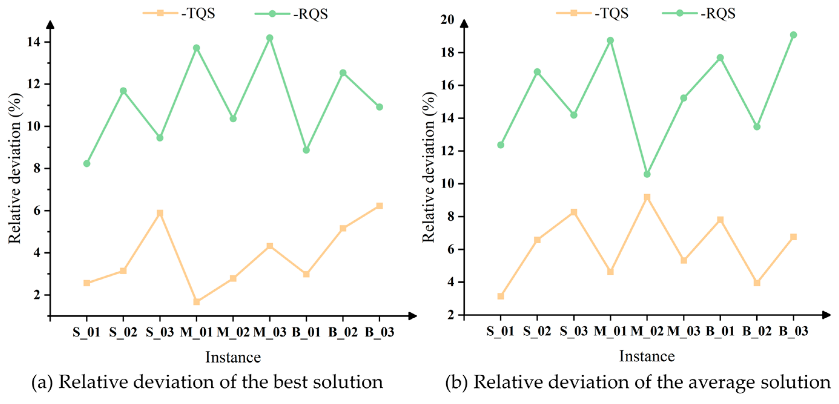
Furthermore, in order to verify the validity of the neighborhood structures designed in the shaking step and the local search step, we carried out the following experiments. Sequentially, the neighborhood structures of the corresponding steps are removed in the VNS algorithm, and then 20 experiments are carried out, respectively, and the best solution, denoted as ${Obj}_B^V$, and the average solution, denoted as ${Obj}_A^V$, are recorded. Their relative deviations, denoted as $R_i$, from the results in Table 7 are calculated using Equation (41). The experiment selects the first instance from each scale within the A1 set. 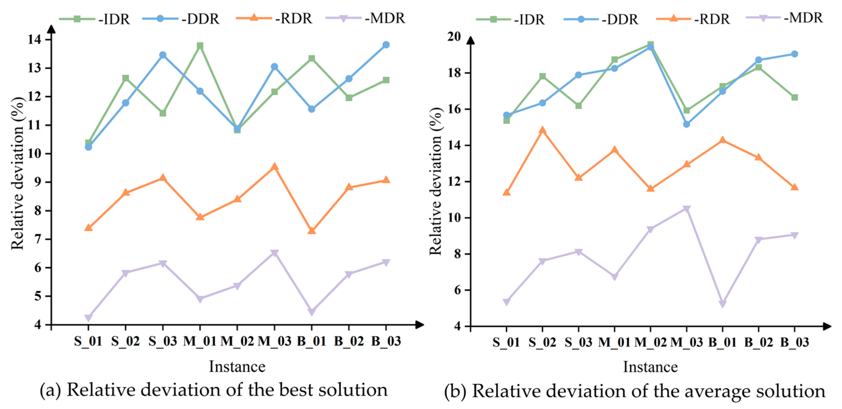The results are presented in Figure 7 and Figure 8, where ‘-’ represents the removal of the corresponding neighborhood structure.

$$R_i={\displaystyle \frac{{Obj}_i^V-{Obj}_G}{{Obj}_G}}\times 100\%,i=\left\{A,B\right\}$$

(41)

The results in Figure 7 and Figure 8 visualize the role played by the neighborhood structure during shaking steps and local search steps in the VNS algorithm process. In the shaking step, the Random QC Profile (RQS) neighborhood structure exerts the greatest impact, with the Time-Increased QC Profile (TQS) structure following. This is because the RQS structure can escape local optima and has a notable effect on improving the solution, while most vessels tend to serve with shorter handling times to minimize the risk of delayed departures. Although the effect of the TQS neighborhood structure is less pronounced than that of the RQS, it still contributes positively to the improvement of the solution. Regarding the local search neighborhood structures, the Idle Destroy–Repair (IDR) and Delay Destroy–Repair (DDR) structures exhibit the most significant and comparable effects, followed by the Random Destroy–Repair (RDR), with the Max-QC Destroy–Repair (MDR) structure having the least impact.

Therefore, in the actual scheduling process, special attention should be given to ships with delays and longer waiting times. Additionally, it is undesirable to select a QC profile with longer handling times solely to meet the maximum number of QC limitation, as this may lead to delayed departures, resulting in higher costs due to delayed times.

In addition, when allocating QC profiles based on the ship–berth sequence discussed in Section 4.3, we introduced a QC profile sorting algorithm. The following presents a comparison of the algorithmic effects of applying versus not applying this QC profile sorting algorithm. When the sorting algorithm is not applied, the first QC profile from the provided set is selected for allocation to the corresponding ship, which significantly increases the randomness in the selection of QC profiles. For the experiment, the first instance from each scale in the A1 set is selected.

Specifically, the QC profile sorting algorithm is removed initially, and then the VNS algorithm, without the sorting component, is executed 20 times to record both the average solution and the average solution time. The results are presented in

Table 9. Comparison results of the QC profile sorting algorithm for instance in A1.

Instance	VNS-		VNS+
	${\mathit{O}\mathit{b}\mathit{j}}_{\mathit{A}}^{{\mathit{V}}^{-}}$	Time(s)	${\mathit{O}\mathit{b}\mathit{j}}_{\mathit{A}}^{{\mathit{V}}^{+}}$	Time(s)
S_01	23,000	11.73	23,000	1.67
S_02	22,000	12.11	22,000	1.83
S_03	22,000	11.58	22,000	1.95
M_01	36,000	22.63	36,000	5.84
M_02	35,000	23.08	35,000	4.92
M_03	33,000	21.89	33,000	7.85
B_01	46,000	38.47	46,000	12.67
B_02	46,000	36.12	46,000	14.43
B_03	44,000	40.03	44,000	15.89

. In Table 9, “VNS+” refers to VNS with the QC profile sorting algorithm, while “VNS-” denotes VNS without the QC profile sorting algorithm.

As shown in Table 9, for each instance, the objective value remains the same regardless of whether the QC profile sorting algorithm is applied. However, the running time of VNS with the QC profile sorting algorithm is significantly shorter than that of VNS without it, indicating that the QC profile sorting algorithm effectively improves computational efficiency and significantly reduces the required computation time. In conclusion, the application of the QC profile sorting algorithm does not affect the final solution’s value but can significantly reduce the running time. Thus, the use of the QC profile sorting algorithm enhances computational efficiency and reduces time costs in practical applications.

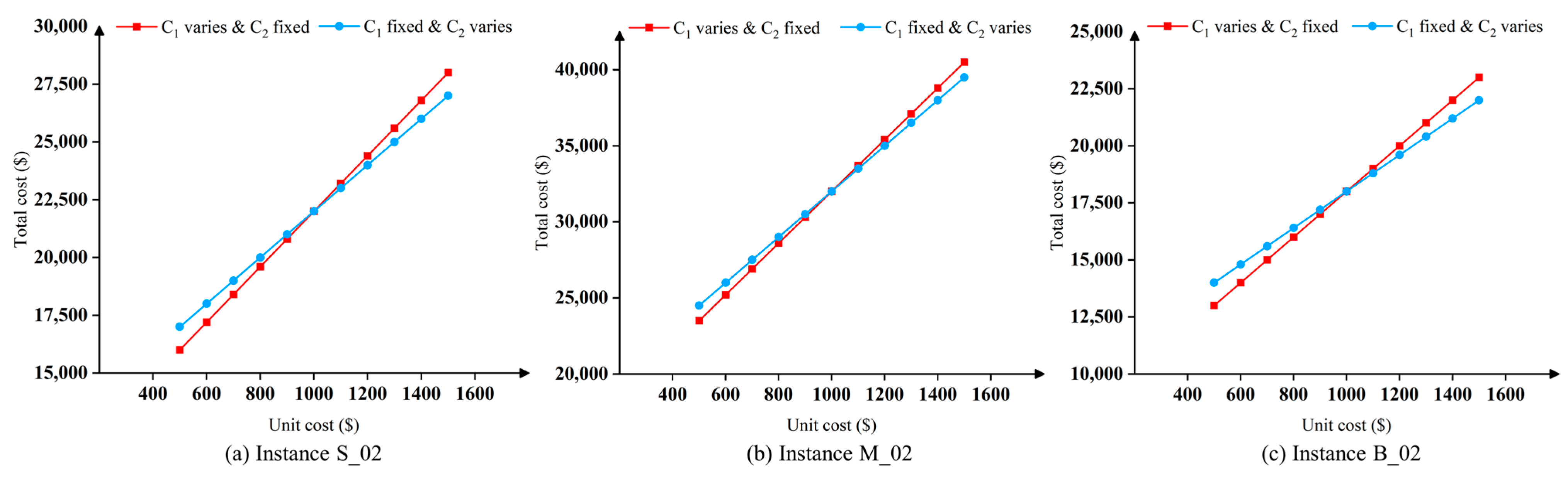
5.2. Sensitivity Analysis of Idle Cost and Delay Cost

In the BACAP model, the unit idle time cost due to vessel waiting $c_i^1$ and the unit delay time cost due to late vessel departures $c_i^2$ are important factors. In this section, a sensitivity analysis is conducted to examine the influence of these costs on the BACAP. The experiment selects the S_02, M_02, and B_02 instances from A1, with the results for these instances presented in Figure 9a–c. In this experiment, $c_i^2$ is first fixed at 1000, and $c_i^1$ is varied by conducting 10 experiments in steps of 100 within the interval [500, 1500]. Then, $c_i^1$ is fixed at 1000, and $c_i^2$ is varied similarly, as well as in steps of 100 within the same interval. Figure 9 illustrates the average total of vessel idle time costs and delay time costs, according to the best solution from 20 runs of the VNS.

The sensitivity analysis results in Figure 9 indicate that with the same step size of cost change, as $c_i^1$ increases, the total cost for each instance (S_02, M_02, and B_02) rises by a larger magnitude and exhibits a steeper slope. In contrast, the increase in total cost when $c_i^2$ is varied is relatively small, with a flatter slope.

The underlying reason for this trend is that, under the data of the A1 instances, the disturbance to the overall operation caused by delayed vessel berthing is greater than that caused by delayed vessel departures. This may be due to the relatively high frequency of delayed vessel berthing, which results in the cost incurred by delayed berthing accounting for a larger portion of the total cost per-unit time. As a result, any change in its cost per unit of time has a significant impact on the total cost. In contrast, delayed vessel departures cause relatively mild disruptions to the overall operation, or occur less frequently, leading to a weaker impact on the total cost from changes in the unit time cost.

Based on the above analysis, in practical management, emphasis should be placed on monitoring the unit time cost associated with delayed berthing. The risk of delayed berthing can be mitigated by training crew members to improve operational skills, upgrading equipment to enhance reliability, and addressing error-causing factors in the berthing process. Optimizing the berthing process, improving the scheduling system, and strengthening communication and collaboration among all parties can further reduce the likelihood of delayed berthing. Additionally, it is crucial to establish a dynamic cost evaluation mechanism to adjust operational strategies and budgets based on real-time cost fluctuations, thereby ensuring maximum economic benefits.

6. Conclusions

This paper investigates the Berth Allocation and Quay Crane Assignment Problem from the perspective of QC profiles, as proposed by Giallombardo et al. [19]. QC profiles offer new insights into the BACAP at the tactical level, with the goal of dealing with existing challenges and improving maritime transportation efficiency. Drawing on previous studies [19,21], we propose a MILP model for the BACAP, with the objective of minimizing the sum of idle time cost due to vessel waiting and delay time cost resulting from late vessel departures. Furthermore, we introduce a VNS algorithm designed to address the BACAP with both stability and effectiveness, particularly suitable for large-scale and complex scheduling problems. Both the model and the algorithm focus on the variable number of QCs in actual terminal operations, providing better applicability for real-world scenarios.

Numerical experiments conducted on the A1 and A2 instance sets validate the stability and efficiency of the proposed VNS algorithm across different problem scales. Specifically, the VNS algorithm outperforms the commercial solver Gurobi in terms of both solution quality and computational time on large-scale instances, achieving high-quality solutions within significantly shorter times. Additionally, the evaluation of the VNS neighborhood structures reveals that different neighborhood structures play distinct roles in the optimization process, and the proposed QC profile sorting algorithm significantly improves the computational efficiency of the VNS without compromising the solution quality. Sensitivity analysis of the per-unit time costs for delayed berthing and delayed departure shows that changes in the unit time cost for delayed berthing have a more pronounced impact on the total cost, highlighting the critical importance of minimizing vessel waiting times in practical port management. Based on this analysis, it is recommended that port operation management prioritize the cost of delayed berthing unit time, mitigate the risk of delayed berthing through crew training and equipment upgrades, optimize the berthing process, and implement a dynamic cost assessment mechanism to adjust operational strategies and budgets in response to cost fluctuations.

In conclusion, this study demonstrates the effectiveness of the VNS algorithm in solving the BACAP. By minimizing vessel idle times and reducing inefficient quay crane reallocations, the proposed framework helps lower energy consumption and emissions, thereby contributing to greener and more sustainable port operations. However, port operations continuously face challenges and developmental bottlenecks. It should be noted that the proposed model is tailored for container terminals, as quay crane operation time is determined by the vessel’s handling volume and the unit-time handling efficiency of a single quay crane. This implies an approximate linear relationship between handling volume and operation time, which is more applicable to container terminals. As a result, the applicability of the current model is limited to container ports.

Future research will explore more generalized and flexible relationships between handling volume and handling time, aiming to extend the model to other types of ports. In the future, we will further consider equipment maintenance strategies in the scheduling model to enhance its practical applicability. Future research can also explore the integration of additional port resources, such as yards and transport trucks, into the BACAP for integrated scheduling from the perspective of the QC profile. Furthermore, extending the BACAP to the coordinated scheduling of multiple ports by considering the cooperation of port groups is a promising research direction. Incorporating sustainability metrics, such as carbon emissions and energy efficiency, into future BACAP formulations will be essential for aligning port operations with global environmental goals. Additionally, incorporating vessel emissions in port operations aligns with the growing emphasis on environmentally sustainably shipping. Lastly, the continuous development of more efficient solution algorithms to address increasingly complex port scheduling problems will remain a key research topic.

References

1. Macioszek, E.; Jurdana, I. Transport of goods on the example of a selected section of transport in Poland. Sci. J. Silesian Univ. Technology. Ser. Transp. 2023, 121, 127–140. [Google Scholar] [CrossRef]
2. Imai, A.; Chen, H.C.; Nishimura, E.; Papadimitriou, S. The simultaneous berth and quay crane allocation problem. Transp. Res. Part E Logist. Transp. Rev. 2008, 44, 900–920. [Google Scholar] [CrossRef]
3. Meisel, F.; Bierwirth, C. Heuristics for the integration of crane productivity in the berth allocation problem. Transp. Res. Part E Logist. Transp. Rev. 2009, 45, 196–209. [Google Scholar] [CrossRef]
4. Iris, Ç.; Pacino, D.; Ropke, S.; Larsen, A. Integrated berth allocation and quay crane assignment problem: Set partitioning models and computational results. Transp. Res. Part E Logist. Transp. Rev. 2015, 81, 75–97. [Google Scholar] [CrossRef]
5. Wang, T.; Wang, X.; Meng, Q. Joint berth allocation and quay crane assignment under different carbon taxation policies. Transp. Res. Part B Methodol. 2018, 117, 18–36. [Google Scholar] [CrossRef]
6. Wang, C.; Miao, L.; Zhang, C.; Wu, T.; Liang, Z. Robust optimization for the integrated berth allocation and quay crane assignment problem. Nav. Res. Logist. (NRL) 2024, 71, 452–476. [Google Scholar] [CrossRef]
7. Sharifi, S.; Gholami, H. A new multi-objective model for berth allocation and quay crane assignment problem with speed optimization and air emission considerations (A case study of Rajaee Port in Iran). Int. J. Marit. Technol. 2023, 17, 25–48. [Google Scholar] [CrossRef]
8. Cheimanoff, N.; Fontane, F.; Kitri, M.N.; Tchernev, N. Exact and heuristic methods for the integrated berth allocation and specific time-invariant quay crane assignment problems. Comput. Oper. Res. 2022, 141, 105695. [Google Scholar] [CrossRef]
9. Correcher, J.F.; Alvarez-Valdes, R.; Tamarit, J.M. New exact methods for the time-invariant berth allocation and quay crane assignment problem. Eur. J. Oper. Res. 2019, 275, 80–92. [Google Scholar] [CrossRef]
10. Ji, B.; Huang, H.; Samson, S.Y. An enhanced NSGA-II for solving berth allocation and quay crane assignment problem with stochastic arrival times. IEEE Trans. Intell. Transp. Syst. 2022, 24, 459–473. [Google Scholar] [CrossRef]
11. Bouzekri, H.; Alpan, G.; Giard, V. Integrated Laycan and Berth Allocation and time-invariant Quay Crane Assignment Problem in tidal ports with multiple quays. Eur. J. Oper. Res. 2021, 293, 892–909. [Google Scholar] [CrossRef]
12. Xiang, X.; Chang, X.; Gong, L.; Liu, X. An innovative framework for optimizing discrete berth allocation and quay crane assignment problems. Comput. Ind. Eng. 2025, 200, 110827. [Google Scholar] [CrossRef]
13. Ji, B.; Tang, M.; Wu, Z.; Yu, S.S.; Zhou, S.; Fang, X. Hybrid rolling-horizon optimization for berth allocation and quay crane assignment with unscheduled vessels. Adv. Eng. Inform. 2022, 54, 101733. [Google Scholar] [CrossRef]
14. Ji, B.; Song, Y.; Samson, S.Y.; Wei, Q. A modified adaptive large neighborhood search algorithm for solving the multi-port continuous berth allocation problem with vessel speed optimization. Comput. Ind. Eng. 2024, 198, 110699. [Google Scholar] [CrossRef]
15. Song, Y.; Ji, B.; Samson, S.Y. Multi-Port Berth Allocation and Time-Invariant Quay Crane Assignment Problem with Speed Optimization. IEEE Trans. Intell. Transp. Syst. 2024, 26, 128–142. [Google Scholar] [CrossRef]
16. Park, Y.M.; Kim, K.H. A scheduling method for berth and quay cranes. OR Spectr. 2003, 25, 1–23. [Google Scholar] [CrossRef]
17. Raa, B.; Dullaert, W.; Van Schaeren, R. An enriched model for the integrated berth allocation and quay crane assignment problem. Expert Syst. Appl. 2011, 38, 14136–14147. [Google Scholar] [CrossRef]
18. Li, F.; Sheu, J.B.; Gao, Z.Y. Solving the continuous berth allocation and specific quay crane assignment problems with quay crane coverage range. Transp. Sci. 2015, 49, 968–989. [Google Scholar] [CrossRef]
19. Wang, Z.; Hu, H.; Zhen, L. Berth and quay cranes allocation problem with on-shore power supply assignment in container terminals. Comput. Ind. Eng. 2024, 188, 109910. [Google Scholar] [CrossRef]
20. Guo, L.; Zheng, J.; Du, J.; Gao, Z.; Fagerholt, K. Integrated planning of berth allocation, quay crane assignment and yard assignment in multiple cooperative terminals. Transp. Res. Part E Logist. Transp. Rev. 2024, 183, 103456. [Google Scholar] [CrossRef]
21. Xiang, X.; Liu, C. An almost robust optimization model for integrated berth allocation and quay crane assignment problem. Omega 2021, 104, 102455. [Google Scholar] [CrossRef]
22. Li, Y.; Chu, F.; Zheng, F.; Liu, M. A bi-objective optimization for integrated berth allocation and quay crane assignment with preventive maintenance activities. IEEE Trans. Intell. Transp. Syst. 2020, 23, 2938–2955. [Google Scholar] [CrossRef]
23. Xu, L.S.; Huang, T.; Zhao, B.W.; Gong, Y.J.; Liu, J. Continuous Berth Allocation and Time-Variant Quay Crane Assignment: Memetic Algorithm With a Heuristic Decoding Method. IEEE Trans. Intell. Transp. Syst. 2025, 26, 3387–3401. [Google Scholar] [CrossRef]
24. Zou, Y.; Xu, P.; Dai, H.; Song, H.; Luo, W. Swarm Optimization with Intra-and Inter-Hierarchical Competition for Large-Scale Berth Allocation and Crane Assignment. IEEE Trans. Emerg. Top. Comput. Intell. 2025, 9, 1307–1321. [Google Scholar] [CrossRef]
25. Ran, L.; Liu, B.; Zhang, G.; Cheng, Y. An improved particle swarm optimization algorithm for berth allocation and time-variant quay crane scheduling problem during an emergency. Expert Syst. Appl. 2025, 269, 126406. [Google Scholar] [CrossRef]
26. Thanos, E.; Toffolo, T.; Santos, H.G.; Vancroonenburg, W.; Vanden Berghe, G. The tactical berth allocation problem with time-variant specific quay crane assignments. Comput. Ind. Eng. 2021, 155, 107168. [Google Scholar] [CrossRef]
27. Malekahmadi, A.; Alinaghian, M.; Hejazi, S.R.; Saidipour, M.A.A. Integrated continuous berth allocation and quay crane assignment and scheduling problem with time-dependent physical constraints in container terminals. Comput. Ind. Eng. 2020, 147, 106672. [Google Scholar] [CrossRef]
28. Zhang, C.; Zheng, L.; Zhang, Z.; Shi, L.; Armstrong, A.J. The allocation of berths and quay cranes by using a sub-gradient optimization technique. Comput. Ind. Eng. 2010, 58, 40–50. [Google Scholar] [CrossRef]
29. Turkogullari, Y.B.; Taskin, Z.C.; Aras, N.; Altinel, I.K. Optimal berth allocation, time-variant quay crane assignment and scheduling with crane setups in container terminals. Eur. J. Oper. Res. 2016, 254, 985–1001. [Google Scholar] [CrossRef]
30. Türkoğulları, Y.B.; Taşkın, Z.C.; Aras, N.; Altınel, İ.K. Optimal berth allocation and time-invariant quay crane assignment in container terminals. Eur. J. Oper. Res. 2014, 235, 88–101. [Google Scholar] [CrossRef]
31. Giallombardo, G.; Moccia, L.; Salani, M.; Vacca, I. Modeling and solving the tactical berth allocation problem. Transp. Res. Part B Methodol. 2010, 44, 232–245. [Google Scholar] [CrossRef]
32. Vacca, I.; Salani, M.; Bierlaire, M. An exact algorithm for the integrated planning of berth allocation and quay crane assignment. Transp. Sci. 2013, 47, 148–161. [Google Scholar] [CrossRef]
33. Xie, F.; Wu, T.; Zhang, C. A branch-and-price algorithm for the integrated berth allocation and quay crane assignment problem. Transp. Sci. 2019, 53, 1427–1454. [Google Scholar] [CrossRef]
34. Tang, X.; Liu, C.; Li, X.; Ji, Y. Distributionally Robust Programming of Berth-Allocation-with-Crane-Allocation Problem with Uncertain Quay-Crane-Handling Efficiency. Sustainability 2023, 15, 13448. [Google Scholar] [CrossRef]
35. Xiang, X.; Lee, L.H.; Chew, E.P. An adaptive dynamic scheduling policy for the integrated optimization problem in automated transshipment hubs. IEEE Trans. Autom. Sci. Eng. 2023, 21, 2701–2715. [Google Scholar] [CrossRef]
36. Yang, Z.; Hu, X.; Li, Y.; Liang, M.; Wang, K.; Wang, L.; Tang, H.; Guo, S. A Q-learning-based improved multi-objective genetic algorithm for solving distributed heterogeneous assembly flexible job shop scheduling problems with transfers. J. Manuf. Syst. 2025, 79, 398–418. [Google Scholar] [CrossRef]
37. Zhang, Z.; Li, X.; Gao, L.; Liu, Q.; Huang, J. Tackling dual-resource flexible job shop scheduling problem in the production line reconfiguration scenario: An efficient meta-heuristic with critical path-based neighborhood search. Adv. Eng. Inform. 2025, 65, 103282. [Google Scholar] [CrossRef]
38. Shao, S.; Xu, G.; Li, J.; Liu, Z.; Jin, Z. A job assignment scheduling algorithm with variable sublots for lot-streaming flexible job shop problem based on NSGAII. Comput. Oper. Res. 2025, 173, 106866. [Google Scholar] [CrossRef]
39. Liu, J.; Tong, L.; Xia, X. A genetic algorithm for vehicle routing problems with time windows based on cluster of geographic positions and time windows. Appl. Soft Comput. 2025, 169, 112593. [Google Scholar] [CrossRef]
40. Su, Y.; Zhang, S.; Zhang, C. A lightweight genetic algorithm with variable neighborhood search for multi-depot vehicle routing problem with time windows. Appl. Soft Comput. 2024, 161, 111789. [Google Scholar] [CrossRef]
41. Wang, C.; Liu, K.; Zhang, C.; Miao, L. Distributionally robust chance-constrained optimization for the integrated berth allocation and quay crane assignment problem. Transp. Res. Part B Methodol. 2024, 182, 102923. [Google Scholar] [CrossRef]
42. Li, B.; Afkhami, P.; Khayamim, R.; Borowska-Stefańska, M.; Wiśniewski, S.; Fathollahi-Fard, A.M.; Ozkul, S.; Dulebenets, M.A. An intelligent hyperheuristic algorithm for the berth allocation and scheduling problem at marine container terminals. Transp. Res. Part E Logist. Transp. Rev. 2025, 198, 104104. [Google Scholar] [CrossRef]
43. Hansen, P.; Mladenović, N. Variable neighborhood search: Principles and applications. Eur. J. Oper. Res. 2001, 130, 449–467. [Google Scholar] [CrossRef]
44. Qian, B.; Feng, F.L.; Yu, N.K.; Hu, R.; Chen, Y.W. An alternating direction multiplier method with variable neighborhood search for electric vehicle routing problem with time windows and battery swapping stations. Appl. Soft Comput. 2024, 166, 112141. [Google Scholar] [CrossRef]
45. Yildiz, S.T.; Ozcan, S.; Cevik, N. Variable neighborhood search-based algorithms for the parallel machine capacitated lot-sizing and scheduling problem. J. Eng. Res. 2023, 13, 100145. [Google Scholar] [CrossRef]
46. Wagner, S.; Mönch, L. A variable neighborhood search approach to solve the order batching problem with heterogeneous pick devices. Eur. J. Oper. Res. 2023, 304, 461–475. [Google Scholar] [CrossRef]
47. Courant, R. Variational Methods for the Solution of Problems of Equilibrium and Vibrations; Lecture Notes in Pure and Applied Mathematics; CRC Press: Boca Raton, FL, USA, 1994; Available online: https://www.taylorfrancis.com/chapters/edit/10.1201/b16924-5/variational-methods-solution-problems-equilibrium-vibrations (accessed on 20 April 2025).
Figure 1. Diagram of the BACAP.
Sustainability 17 04022 g001
Figure 2. An illustrative example of constraint (5).
Sustainability 17 04022 g002
Figure 3. A schematic instance for Constraint (23).
Sustainability 17 04022 g003
Figure 4. Flowchart of VNS framework for solving the BACAP.
Sustainability 17 04022 g004
Figure 5. Diagram of the vessel conflict adjustment. Note: Red highlights the vessel conflict, while black indicates feasible berthing schedules.
Sustainability 17 04022 g005
Figure 6. Diagram of the repair process. Note: Red indicates the vessel to be inserted, black represents the original berthing schedule, and yellow highlights the time period where conflicts may occur.
Sustainability 17 04022 g006
Figure 7. Shaking neighborhood structure effect experiments results.
Sustainability 17 04022 g007
Figure 8. Local search neighborhood structure effect experiments results.
Sustainability 17 04022 g008
Figure 9. Results of VNS under various c i 2 and c i 2 .
Sustainability 17 04022 g009