Abstract
Due to the inherent complexity of urban road networks and the irregular periodic fluctuations of traffic flow, traffic forecasting remains a challenging spatiotemporal modeling task.Existing studies predominantly focus on capturing spatial dependencies among nodes, while often overlooking the long-term evolutionary patterns and internally stable, recurring flow behaviors at individual nodes. This limitation compromises both the generalization capacity and long-term forecasting performance of current models.To address these issues, we propose a novel Dynamic Pattern Matching Network (DPMNet) that incorporates a memory-augmented architecture to dynamically learn and retrieve historical traffic patterns at each node, thereby enabling efficient modeling of localized flow dynamics. Building upon this foundation, we further develop a comprehensive framework named DPMformer, which integrates daily and weekly temporal embeddings to enhance the modeling of long-term trends and leverages a pattern matching mechanism to improve the representation of complex spatiotemporal structures.Extensive experiments conducted on four real-world traffic datasets demonstrate that the proposed method significantly outperforms mainstream baseline models across multiple forecasting horizons and evaluation metrics.
1. Introduction
With the rapid advancement of urbanization and the development of intelligent transportation systems, achieving efficient and environmentally friendly mobility has become a key issue for sustainable urban development. Among various strategies, accurate traffic flow forecasting plays a vital role in supporting traffic scheduling optimization and the rational allocation of transportation resources, thereby contributing to congestion mitigation, energy conservation, and carbon emission reduction. However, the task remains highly challenging due to the inherent complexity of urban road networks and the irregular yet periodic spatiotemporal patterns exhibited by traffic flow. Traditional methods such as the Historical Average (HA) [1], Autoregressive Integrated Moving Average (ARIMA) [2], Vector Autoregression (VAR) [3], and Support Vector Regression (SVR) [4] methods, though widely applied in earlier studies, heavily rely on manual feature engineering. These approaches are costly to develop and often exhibit poor generalization when faced with complex traffic dynamics, making them inadequate for meeting the growing demands for real-time and accurate forecasting in modern intelligent transportation systems.
With the development of deep learning, methods based on Recurrent Neural Networks (RNNs), proposed by Li et al. [5] and Lai et al. [6], have been introduced. RNNs can effectively capture temporal periodicity. However, traffic flow contains complex spatiotemporal dependencies, and merely capturing temporal dependencies is insufficient. To address this, researchers have proposed Graph Convolutional Networks (GCNs) [7,8,9] to capture spatial dependencies within road networks. These methods effectively consider both spatial and temporal characteristics and often achieve promising results; as a result, they have become the mainstream approach. However, current methods still possess the following limitations:
(1) Lack of long-term trend modeling capability. Most existing methods [10,11,12] rely on short historical traffic sequences (e.g., 12 time steps, approximately one hour), which limits a model’s temporal perception and hinders its ability to capture long-term evolving patterns in traffic flow. As shown in the text of Figure 1, the same traffic node often exhibits a highly consistent flow pattern on weekdays and another relatively stable but noticeably different pattern on weekends. This indicates the presence of stable and structured long-term trends in traffic dynamics.
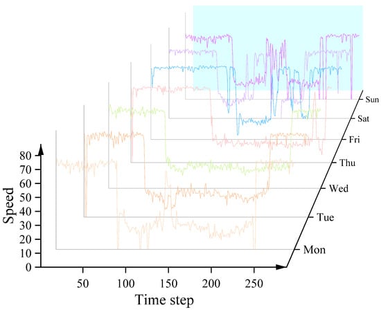
Figure 1.
Similar traffic characteristics within a single node.
(2) Neglect of intra-node traffic pattern regularities. Existing studies primarily focus on spatial dependencies across different nodes [13,14,15] while paying insufficient attention to the repetitive structural information embedded in the temporal evolution of individual nodes. In practice, traffic nodes often exhibit strong periodic behaviors—for example, travel patterns on weekdays differ significantly from those on weekends. Effectively identifying and leveraging such structural flow patterns can enhance a model’s generalization ability and prediction accuracy under varying temporal conditions.
To address the above challenges, we propose a novel Dynamic Pattern Matching Network (DPMNet). This network incorporates a memory module capable of storing and dynamically updating representative features over extended time horizons, enabling the model to perceive long-term temporal variations. Furthermore, we introduce daily and weekly temporal embeddings to encode time-specific features at multiple granularities, thereby enhancing the model’s ability to recognize evolving traffic patterns over different time scales. Based on these mechanisms, we build a complete prediction framework named DPMformer, which integrates node-level dynamic pattern learning, long-term trend modeling, and multi-scale temporal awareness for accurate traffic flow forecasting.
The main contributions of this work are summarized as follows:
- We reformulate the task of capturing spatiotemporal dependencies via Graph Convolutional Networks (GCNs) into a dynamic pattern matching framework. This allows our model to better distinguish node-specific characteristics and reduces reliance on the static topology of the road network, making it more adaptable to varying spatial and flow distribution patterns across traffic nodes.
- We propose a novel Dynamic Pattern Matching Network (DPMNet), which leverages a memory module to store representative patterns over long temporal ranges. These patterns encapsulate both long-term traffic trends and intra-node flow regularities, enhancing the model’s capacity for long-term traffic prediction.
- Based on DPMNet, we develop a comprehensive forecasting framework, DPMformer, and conduct extensive experiments on four real-world traffic datasets. Our results demonstrate that DPMformer significantly outperforms existing baseline methods in prediction accuracy, validating the effectiveness and generalizability of our approach.
2. Related Work
2.1. Traffic Flow Prediction
Statistical methods such as the Historical Average (HA) [1], Auto-Regressive Integrated Moving Average (ARIMA) [2], and traditional machine learning techniques like Vector Auto-Regression (VAR) [3] and Support Vector Regression (SVR) [4] method were among the early approaches for traffic flow prediction. However, these methods suffer from notable drawbacks, including their inability to capture complex nonlinear relationships, limited robustness in the face of sudden events, and weak generalization ability, which restricts their accuracy in forecasting. In recent years, the development of deep learning has led to significant breakthroughs in traffic flow prediction. For example, Lai et al. [6] utilized Recurrent Neural Networks (RNNs) to capture temporal characteristics; however, such models lack the ability to capture the complex spatiotemporal dependencies in traffic flow data. Subsequently, Jiang et al. [16] divided road network images into grids and used Convolutional Neural Networks (CNNs) to extract spatial features.
However, researchers soon realized that CNNs were inefficient at modeling spatial structures, leading them to adopt the more efficient Graph Convolutional Networks (GCNs), which has since become the mainstream approach. To date, GCN-based methods have led to a series of new studies. Agafonov [17] and Fukuda et al. [18] extracted spatial features using static graphs, which are well suited for represent connections and distances between nodes. However, static graphs, often based on predefined spatial features, struggle to effectively express unique geographical characteristics. For instance, the traffic patterns in commercial areas and suburban areas can differ significantly, yet these differences cannot be solely captured by node distances. To address this, Bai et al. [19] turned to adaptive graphs that can modify their parameters during model training via backpropagation, allowing for more flexible representation of spatial relationships. However, the spatial and temporal characteristics of traffic flow are interdependent. Temporal features are influenced by spatial characteristics, and spatial features change over time, making it difficult for adaptive graphs to represent spatiotemporal dependencies.
In recent years, dynamic graph structures have attracted widespread attention in the field of traffic flow forecasting due to their ability to dynamically capture spatiotemporal dependencies that evolve over time. Zhou et al. [20] proposed the Graph Convolutional Recurrent Network (GCRN), which integrates graph convolution with gated recurrent units to jointly model the spatiotemporal evolution of traffic flow. Liang et al. [21] introduced the Dynamic Spatiotemporal Graph Convolutional Recurrent Network (DST-GCRN) for traffic prediction. By incorporating dynamic graph convolutional layers, this method effectively models time-varying spatial dependencies while leveraging recurrent neural networks to capture temporal patterns in traffic dynamics.Additionally, Shao et al. [22] proposed D2STGNN, which decouples spatiotemporal data into intrinsic and diffusion components to further enhance prediction accuracy. However, most of these methods focus primarily on modeling inter-node spatiotemporal dependencies, with relatively little attention paid to learning and extracting traffic patterns within individual nodes.
2.2. Neural Memory Networks
Neural memory networks were initially introduced in the field of natural language processing (NLP), particularly within sequence-to-sequence (seq2seq) models, where they enhanced the ability to capture long-term dependencies through external memory mechanisms. Weston et al. [23] first proposed the Memory Network framework to improve the accuracy of question-answering systems. Their approach introduced an external storage module capable of retaining information, thereby enabling neural networks to handle more complex long-range dependency tasks. Sukhbaatar et al. [24] later introduced the End-to-End Memory Network, which improved the learning mechanism by allowing the model to optimize the memory content directly during training. This end-to-end optimization significantly enhanced the model’s memory capabilities across various tasks. Madotto et al. [25] further extended this idea by incorporating a multi-hop attention mechanism into the memory network, enabling multi-step reasoning and thereby boosting the model’s performance in complex inference scenarios.
Memory networks have also found wide application in computer vision. Yang et al. [26] applied memory networks to object tracking, demonstrating their effectiveness in handling dynamic visual information. Oh et al. [27] employed memory networks for object segmentation tasks, achieving more precise segmentation results. In time series forecasting, Cheng et al. [28] applied memory networks to multivariate time series prediction, showing significant improvements on high-dimensional temporal data and confirming the strong potential of memory mechanisms in temporal modeling.
In the context of traffic flow forecasting, memory networks have also gained increasing attention. Lee et al. [29] proposed a Graph Convolutional Memory Network (GC-MemNet) that integrates graph convolution with memory modules to learn representative traffic patterns with similar spatiotemporal features. This approach effectively captures complex spatiotemporal dependencies among traffic nodes and enhances the ability to model long-term trends in traffic flow. Jiang et al. [30] developed a meta-graph learner inspired by memory networks; their network stores dynamic graphs and captures heterogeneity in spatiotemporal patterns—an essential capability for addressing spatial heterogeneity and temporal variability in traffic systems. Furthermore, Peng et al. [31] introduced MA-GCN, a Memory-Augmented Graph Convolutional Network that utilizes a memory module to store historical traffic patterns and improves the model’s representational power in traffic prediction tasks. Liu et al. [32] proposed a Spatiotemporal Memory-Augmented Multi-Level Attention Network that combines multi-level attention mechanisms with memory modules, further enhancing predictive accuracy and robustness.Inspired by these advances, we propose a memory-based architecture with explicit storage capability to differentiate and preserve representative traffic patterns within individual nodes. Unlike existing methods that primarily rely on inter-node spatiotemporal dependencies, our model emphasizes intra-node periodic traffic behaviors. This design allows the model to capture long-term trends more effectively, thereby significantly improving both its accuracy and its generalization capacity in traffic flow forecasting.
3. Methodology
In this section, we provide a detailed explanation of the proposed model. The overall framework of the model, illustrated in Figure 2, consists of an encoder and a decoder. The Dynamic Pattern Matching Network is the core structure, and all components will be described in detail in the following sections.
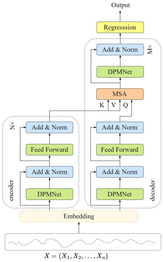
Figure 2.
Overall structure of DPMformer.
3.1. Encoder and Decoder Structure
Encoder: The encoder consists of N identical stacked layers, each containing two submodules. The first submodule is NL-DPMNet, followed by a feed-forward module composed of two fully connected layers. Both submodules employ residual connections [33] and layer normalization [34].
Here, X represents the input to each submodule, and sublayer denotes the function of the submodule.
Decoder: The decoder consists of M identical stacked layers, each containing three submodules. The key difference from the encoder is the inclusion of a multi-head self-attention module. This module performs multi-head attention over the encoder’s output. As with the encoder, all modules in the decoder use residual connections and layer normalization.
3.2. Embedding Layer
Traffic flow data exhibit pronounced periodic characteristics, typically manifesting as recurring patterns on daily and weekly scales. To effectively capture these temporal variations, we introduce a time-tag-based embedding mechanism by constructing two learnable embedding matrices. Specifically, denotes the daily embedding, where corresponds to the number of time steps in a single day, facilitating the modeling of intra-day traffic fluctuations such as morning and evening rush hours. Likewise, represents the weekly embedding, where captures the seven days of a week, enabling the model to differentiate between structural flow patterns across weekdays and weekends.Each time step t is first mapped into a temporal vector using the embedding function , based on its associated date tag (including both an intra-day time index and a day-of-week index), as shown in Equation (2):
where represents the historical input data, where N is the number of nodes, L is the length of the time steps, and d denotes the number of channels. represents the embedding function. After obtaining the daily embedding and the weekly embedding, the two are combined into a new temporal embedding:
Here, Cat denotes the concatenation operation, and represents the temporal label that encompasses both the time steps within a day and the days of the week. To capture more features from the historical data, X is linearly projected into a higher-dimensional space:
Here, , Map represents the projection function. Finally, the temporal embedding and the high-dimensional historical input are combined:
Here, represents the historical input data embedded with temporal labels.
3.3. Dynamic Pattern Matching Network
To dynamically store and retrieve similar traffic patterns, we have designed the Dynamic Pattern Matching Network as shown in Figure 3. First, we enhance the representational capability of historical traffic data by using a Multi-Layer Perception (MLP):
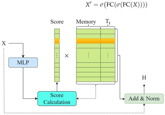
Figure 3.
Overview of DPMNet.
Here, denotes a fully connected layer, and represents an activation function (e.g., ReLU). The memory tensor is a fully learnable parameter used to store representative historical traffic patterns for each node. In this context, W denotes the number of memory slots per node, N is the number of nodes, and H is the dimensionality of each memory item. Notably, , allowing the memory to store a broader range of historical patterns than the current input sequence alone. During training, the memory is initialized using the Xavier initialization method and is continuously optimized via gradient updates as part of the network parameters.Each node is assigned an independent set of memory vectors (node-wise design), enabling the model to capture its unique long-term periodicity and evolutionary trends. The memory parameters are shared across all training batches to facilitate efficient representation learning and enhance generalization ability.
Traffic flow data exhibit strong temporal dependencies and regularities. The time embeddings introduce additional feature dimensions for each time step, allowing the model to recognize the temporal position within a day or week, thereby enhancing its sensitivity to temporal information. Since the memory module itself is not inherently time-aware, we incorporate the temporal embedding introduced in Section 3.2 into the memory input to enhance its temporal sensitivity. Subsequently, we compute similarity scores between the temporally enhanced historical input and the memory representations.
where is the time slot embedding matrices generated by the time embedding layer. denotes the concatenation operation, and is the instance of the Memory after merging the time embeddings. The symbol ⊙ represents the Hadamard product. The score represents the computed similarity score. Using this score, we retrieve the traffic patterns stored in the Memory and perform a residual connection with the original historical data. After applying layer normalization, we obtain the output of DPMNet:
3.4. Multi-Head Self-Attention Module
To enhance the model’s ability to capture historical traffic patterns, we adopt structurally identical but functionally distinct encoder and decoder modules. This design improves the modeling of global dependencies and reduces the impact of anomalous data on prediction outcomes. The encoder aggregates key information from historical time steps using a multi-head attention mechanism, while the decoder dynamically integrates the global context captured by the encoder with the current state of the prediction sequence, thereby improving both the accuracy and stability of the forecast. In our model, we utilize the standard Transformer multi-head attention module [35], but without incorporating positional encoding. This mechanism enables the model to identify critical time steps with predictive significance under varying delays (e.g., transitional periods before rush hours or unexpected events), thus enhancing its adaptability to both non-stationary and periodic patterns. The attention mechanism is computed as follows:
where K and V are outputs from the encoder, Q is the output from the first half of the decoder, and is the dimensionality of the key vectors. Without relying on an explicit spatial adjacency matrix, this mechanism implicitly learns the relative dependencies among different nodes and their historical states, thus enabling the modeling of spatial correlations in a data-driven and flexible manner.
3.5. Regression Layer
The regression layer projects the intermediate output features of the model into the target variable space. This projection not only adjusts the shape of the output but also ensures that the output’s value range and distribution meet the task requirements. The design is as follows:
where represents the ReLU activation function.
4. Experiments
4.1. Datasets and Settings
Datasets: To evaluate the proposed DPMformer model, extensive experiments were conducted on four real-world datasets, following the approach of previous works [5,7]:
- METR-LA: This dataset consists of traffic speed data recorded by 207 sensors on highways in Los Angeles. It spans four months, starting from March 2012.
- PEMS-BAY: Collected by the California Department of Transportation (CalTrans), this dataset includes readings from 325 sensors over the period from 1 January 2017, to 31 May 2017.
- PEMSD7 (M) and PEMSD7 (L): These datasets represent traffic data from California District 7, covering weekdays from May to June 2012. The primary difference between the two lies in the number of sensors used.
Each dataset has a time step of 5 min per day, and the detailed characteristics are listed in Table 1. The datasets were split in chronological order, with 60% for training, 20% for validation, and 20% for testing. Additionally, Z-score normalization was applied for data pre-processing:
where is the mean and is the standard deviation.

Table 1.
Dataset information.
Settings: All experiments were conducted on a server equipped with an NVIDIA GeForce GTX 4090 GPU. The Adam optimizer was used for model optimization, and the Mean Absolute Error (MAE) was chosen as the loss function. Table 2 provides a detailed list of the hyperparameter settings for the model across the four datasets. During training, an early stopping strategy was employed to terminate training and prevent overfitting.
Table 2.
Model parameters for different datasets.
4.2. Baselines
To evaluate the performance of our proposed model, we compare it to the following baseline methods:
- HA [1]: This method uses the historical average as the prediction for future values.
- ARIMA [2]: This method represents the current value of traffic flow as a linear combination of its historical values, and corrects the prediction using a linear combination of past error terms.
- VAR [3]: This extended auto-regressive model is designed for modeling the relationships between multiple variables.
- SVR [4]: This method maps time series data to a high-dimensional feature space and finds the optimal hyperplane for prediction within that space.
- STGCN [7]: This method utilizes graph convolution and 1D convolutional neural networks to separately extract temporal and spatial information.
- DCRNN [5]: This method integrates diffusion convolution into a recurrent neural network to capture both temporal and spatial dependencies.
- GWN [36]: This method designs an adaptive adjacency matrix combined with temporal convolution networks (TCNs) to extract spatiotemporal dependencies.
- ASTGCN [8]: This method combines spatiotemporal attention mechanisms to capture dynamic spatiotemporal correlations in traffic flow.
- STSGCN [9]: This method emphasizes the importance of local spatiotemporal dependencies by understanding the heterogeneity of spatiotemporal data.
- GMAN [37]: This method introduces spatial and temporal attention mechanisms to separately model dynamic spatial and nonlinear temporal correlations.
- STEP [38]: This method designs a pre-training model to learn segment representations from very long historical sequences.
- STGM [39]: This method investigates how the historical information of node i affects the future state of node j for more accurate predictions.
- STAEformer [40]: This method explicitly models the time delay of spatial information propagation, considering the delayed transmission characteristic of traffic flow.
- DDGCRN [41]: This method combines dynamic graphs with RNN architectures to effectively extract spatiotemporal dependencies via a decoupling structure.
- STD-MAE [42]: This method constructs a pre-training framework using two decoupled auto-encoders and integrates them seamlessly to improve performance.
Following the settings of baseline models, we use 12 historical time steps to predict future traffic conditions. By comparing our model with these methods, we further validate the superiority of our approach in spatiotemporal traffic prediction.
4.3. Evaluation Metrics
We selected three widely used evaluation metrics to assess the performance of our model:
MAE (Mean Absolute Error):
RMSE (Root Mean Square Error):
MAPE (Mean Absolute Percentage Error):
where n represents the number of test samples, while and represent the predicted and actual values of the ith element, respectively.
4.4. Overall Performance
The overall performance of the model is presented in Table 3 and Table 4. Bold values indicate the best results, while underlined values represent the second-best results.For fairness in comparison, the results of the baseline models are taken directly from the original literature, which are widely cited in the field of traffic flow prediction. According to the results in the tables, traditional statistical methods and classical machine learning models (such as HA, ARIMA, VAR, and SVR) significantly lag behind deep learning methods in prediction performance. These methods struggle to effectively model the complex spatiotemporal dependencies in traffic flow, particularly when faced with dynamic changes and nonlinear characteristics.
Table 3.
Performance comparison of different models on the METR-LA and PEMS-BAY datasets.
Table 4.
Comparison of performance on the PEMSD7M and PEMSD7L datasets.
In contrast, the attention-based GMAN model is somewhat capable of modeling both temporal and spatial information, but its spatial modeling does not explicitly account for the actual connectivity in the traffic network, which limits further performance improvements. Methods based on Graph Convolutional Networks (GCNs), such as STGCN and STSGCN, utilize the graph structure to model spatial dependencies and generally outperform traditional models and attention-based methods. These models can integrate the structural information of the traffic network, allowing for more effective extraction and fusion of spatiotemporal features.
However, earlier GCN-based methods predominantly use static graph structures, failing to capture the dynamic dependencies that evolve over time in the traffic network. In contrast, dynamic graph methods (such as STGM and STAEformer) introduce dynamic graph modeling mechanisms, which better adapt to the evolving structure of traffic networks over time and significantly improve prediction performance in complex traffic scenarios. Recent pre-trained models (such as STEP and STD-MAE) have demonstrated strong performance in traffic flow forecasting tasks. These methods leverage self-supervised learning mechanisms, such as masked modeling, to enable the model to learn more generalizable features from large-scale unlabeled data.
Our proposed DPMformer outperforms other baseline models in all experiments, primarily due to two design advantages: First, we introduce a node-level memory mechanism that focuses on modeling the traffic flow patterns within each individual node. By modeling and memorizing the historical traffic flow of each node, we can precisely capture these recurring features, making the model more targeted and stable in predictions. Second, we emphasize modeling the long-term trends in traffic flow. Traditional methods often focus on short-term dynamic changes, neglecting the global patterns in the long-term evolution of traffic flow. With the help of the prompt mechanism and memory network, DPMformer effectively preserves key pattern information from the past, enabling the model to better infer future trends and achieve superior results in long-term prediction tasks.
To provide a more comprehensive evaluation of the model’s performance across different prediction horizons, we conducted a step-wise prediction error comparison on the METR-LA dataset for 12 steps (i.e., 60 min), as shown in Figure 4. From the experimental results, it can be observed that in Step 1 (i.e., 5 min prediction), the error of DPMformer is relatively higher, which may be due to the more dramatic short-term traffic state fluctuations. Our model, which emphasizes modeling global trends, may have slightly limited ability to capture fine-grained fluctuations. However, as the prediction horizon increases, we find that the error growth rate of DPMformer is significantly lower than that of the comparison methods. Starting from Step 3, its performance gradually surpasses other models, and it maintains optimal performance across all subsequent prediction steps. This trend indicates that although DPMformer experiences slight losses in the early time steps, its overall prediction error exhibits stronger stability over time, enabling it to capture the medium- and long-term evolution of traffic flow more effectively.
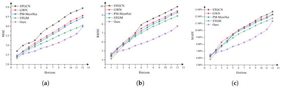
Figure 4.
Twelve-step forecast comparison on the METR-LA dataset. (a) MAE on METR-LA. (b) RMSE on METR-LA. (c) MAPE on METR-LA.
4.5. Ablation Studies
In this section, we conduct an effectiveness analysis of the key components of the model to assess their contributions to the performance of DPMNet. The experimental results are shown in Figure 5, where the RMSE values are magnified by a factor of 100 to better illustrate the performance differences under different settings:
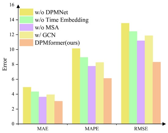
Figure 5.
Ablation study results.
- w/o DPMNet: The DPMNet module is removed and replaced with an MLP with a similar parameter scale, while the time embedding is retained. This setup tests the contribution of the pattern matching capability introduced by DPMNet.
- w/ GCN: DPMNet is replaced with a GCN model containing two graph convolution layers, constructed using a static geographical adjacency matrix to capture spatial dependencies between nodes.
- w/o Time Embedding: The time embedding module is removed to evaluate the model’s reliance on time information for modeling.
- w/o MSA (Multi-Head Self-Attention): The multi-head self-attention module is removed and replaced with a simple feature fusion operation to verify the effectiveness of the attention mechanism in spatiotemporal modeling.
The w/o DPMNet experimental results show that, despite using a similar parameter scale MLP model, the overall performance significantly drops. This indicates that the pattern matching mechanism is crucial for capturing and storing typical traffic patterns. Traffic flow variations at nodes often exhibit strong periodicity and structure, and DPMNet’s ability to automatically recognize and remember these repetitive patterns greatly enhances prediction accuracy.The w/GCN results show that, although graph convolution can leverage spatial structure for modeling, the overall performance is still significantly inferior to that of DPMNet. On the one hand, the receptive field of GCN is limited by the fixed graph structure, leading to restricted information propagation and error accumulation in long-term predictions. On the other hand, GCN uses shared parameters across all nodes, making it difficult to independently model and remember the unique traffic patterns of each node. In contrast, DPMNet adopts a node-wise memory unit design, enabling it to flexibly adapt to the individual characteristics and evolution patterns of each node, offering stronger long-term modeling and generalization capabilities. The w/o Time Embedding experimental results indicate that removing the time embedding results in a significant performance drop, highlighting the critical role of time information in traffic flow prediction. Traffic flow is typically driven by daily and periodic factors, and lacking time perception abilities makes it difficult for the model to capture these trend-like and periodic changes, negatively impacting overall prediction performance.The w/o MSA results show that, while the basic predictive function is maintained, overall performance decreases. This demonstrates that the multi-scale attention mechanism plays a positive role in enhancing the model’s ability to model complex spatiotemporal dynamics. The module effectively aggregates and strengthens key information across different time scales, enabling the model to adapt better and maintain stability when facing variable traffic patterns.
4.6. Hyperparameter Sensitivity Analysis
In this section, we investigate the impact of key hyperparameters on the model’s performance. We conducted comparison experiments for three hyperparameters: hidden dimension, number of encoders, and number of decoders. To better illustrate the results, the MAPE values are scaled by a factor of 100.
4.6.1. Sensitivity to Hidden Dimension
We tested the hidden dimension with values to evaluate its impact on model performance. The results, shown in Figure 6, indicate that the hidden dimension does not have a linear effect on model performance. The best performance is achieved when the hidden dimension is 16, and performance declines as the hidden dimension increases beyond that point.
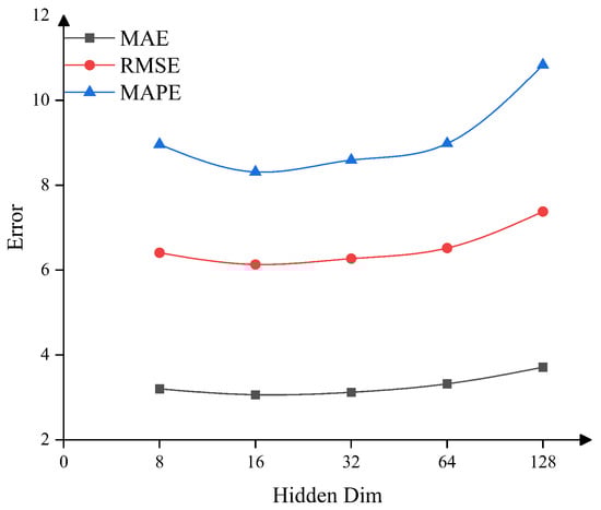
Figure 6.
Sensitivity of the model to hidden dimensions.
4.6.2. Sensitivity to Numbers of Encoders (N) and Decoders (M)
We tested the number of encoders with values , while keeping the number of decoders fixed at M = 1. We then tested the number of decoders with values , while keeping the number of encoders fixed at N = 2. Figure 7 shows that the model’s sensitivity to the number of encoders and decoders is relatively low, with the best result achieved when and .
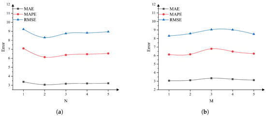
Figure 7.
Sensitivity of the model to the number of N and M. (a) Sensitivity of the model to the number of encoders. (b) Sensitivity of the model to the number of decoders.
4.7. Visualizing Prediction Results
To more intuitively assess the model’s performance under different traffic patterns, we conducted a visual analysis by comparing the predicted results with the actual values, as shown in Figure 8. Due to space limitations, we selected the speed data from sensors 32 and 64 between 4:00 on 8 June 2012, and 4:00 on 9 June 2012, as representatives for display. The experimental results show that our model performs well in predicting future traffic states across different nodes and changing trends. Figure 8a shows the traffic speed data from sensor 32, which exhibits continuous fluctuations. Our model is able to track this trend well and accurately predict medium- to long-term traffic changes. This indicates that the model has strong capabilities in capturing node-level traffic evolution patterns, especially for nodes with clear periodic features and trends, where it exhibits good adaptability. Figure 8b displays the prediction results from sensor 64, where the speed curve exhibits significant fluctuations, including sharp increases and decreases. Although these changes are not caused by sudden events but rather reflect the complex evolution of the traffic system itself, the model maintains relatively stable prediction accuracy, demonstrating its generalization ability in modeling complex patterns. It should be noted that when there is significant noise interference in the data (such as sensor failures resulting in zero readings at certain times), the model’s fit may slightly degrade during those periods. However, this local error is normal and has limited impact on the overall trend modeling.
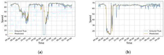
Figure 8.
Visualization of the prediction results on METR-LA. (a) Visualization on sensor 32. (b) Visualization on sensor 64.
5. Conclusions
In this study, we propose an innovative dynamic pattern matching method that transforms the complex spatiotemporal dependency modeling problem in traffic flow into a node-level pattern learning and matching problem. To this end, we design a memory-enhanced dynamic pattern matching network (DPMNet) and construct a complete traffic flow prediction model, DPMformer. This model effectively captures the internal structural flow patterns of nodes by matching the current traffic flow with representative patterns in the memory bank, and enhances long-term trend modeling through daily and weekly embedding mechanisms, thereby achieving accurate predictions of future flow changes. Our experimental results show that DPMformer outperforms existing baseline models on four real-world traffic flow prediction datasets, validating our point that using a few representative patterns to replace a large number of complex traffic patterns for each node is both feasible and effective. Through comparison with existing methods, we demonstrate that DPMformer not only enables efficient and accurate predictions in dynamic traffic environments but also provides crucial support in achieving sustainable urban development goals in traffic flow management. Overall, DPMformer offers a novel and efficient solution to traffic flow prediction problems and provides valuable theoretical and practical guidance for future intelligent transportation systems and sustainable urban development.
Author Contributions
Conceptualization, Y.H. and W.H.; methodology, Y.H.; software, W.H.; validation, W.H., Y.X. and S.W.; formal analysis, Y.H. and S.W.; investigation, S.W.; resources, W.H.; data curation, S.W.; writing—original draft preparation, W.H.; writing—review and editing, Y.H.; visualization, W.H.; supervision, Y.H.; funding acquisition, Y.H. All authors have read and agreed to the published version of the manuscript.
Funding
This research was funded by the National Natural Science Foundation of China, grant number 72061016; the Jiangxi Province Key Laboratory of Multidimensional Intelligent Perception and Control of China, grant number 2024SSY03161; and the Natural Science Foundation Project of Ji’an City, grant number 20244-018595.
Institutional Review Board Statement
Not applicable.
Informed Consent Statement
Not applicable.
Data Availability Statement
The data presented in this study are available on request from the corresponding author.
Conflicts of Interest
Author Wu Shuiqing was employed by the company Jiangxi Yongan Traffic Facilities Technology Co., Ltd. The remaining authors declare that the research was conducted in the absence of any commercial or financial relationships that could be construed as a potential conflict of interest.
References
- Liu, J.; Guan, W. A summary of traffic flow forecasting methods. J. Highw. Transp. Res. Dev. 2004, 21, 82–85. [Google Scholar]
- Zhang, G.P. Time series forecasting using a hybrid ARIMA and neural network model. Neurocomputing 2003, 50, 159–175. [Google Scholar] [CrossRef]
- Williams, B.M.; Hoel, L.A. Modeling and forecasting vehicular traffic flow as a seasonal ARIMA process: Theoretical basis and empirical results. J. Transp. Eng. 2003, 129, 664–672. [Google Scholar] [CrossRef]
- Wu, C.H.; Ho, J.M.; Lee, D.T. Travel-time prediction with support vector regression. IEEE Trans. Intell. Transp. Syst. 2004, 5, 276–281. [Google Scholar] [CrossRef]
- Li, Y.; Yu, R.; Shahabi, C.; Liu, Y. Diffusion Convolutional Recurrent Neural Network: Data-Driven Traffic Forecasting. In Proceedings of the 6th International Conference on Learning Representations, ICLR 2018, Vancouver, BC, Canada, 30 April–3 May 2018. [Google Scholar]
- Lai, G.; Chang, W.C.; Yang, Y.; Liu, H. Modeling long-and short-term temporal patterns with deep neural networks. In Proceedings of the 41st International ACM SIGIR Conference on Research & Development in Information Retrieval, Ann Arbor, MI, USA, 8–12 July 2018; pp. 95–104. [Google Scholar]
- Yu, B.; Yin, H.; Zhu, Z. Spatio-Temporal Graph Convolutional Networks: A Deep Learning Framework for Traffic Forecasting. In Proceedings of the Twenty-Seventh International Joint Conference on Artificial Intelligence, Stockholm, Sweden, 13–19 July 2018; International Joint Conferences on Artificial Intelligence Organization: Washington, DC, USA, 2018; pp. 3634–3640. [Google Scholar] [CrossRef]
- Guo, S.; Lin, Y.; Feng, N.; Song, C.; Wan, H. Attention based spatial-temporal graph convolutional networks for traffic flow forecasting. In Proceedings of the AAAI Conference on Artificial Intelligence, Honolulu, HI, USA, 27 January–1 February 2019; Volume 33, pp. 922–929. [Google Scholar]
- Song, C.; Lin, Y.; Guo, S.; Wan, H. Spatial-temporal synchronous graph convolutional networks: A new framework for spatial-temporal network data forecasting. In Proceedings of the AAAI Conference on Artificial Intelligence, New York, NY, USA, 7–12 February 2020; Volume 34, pp. 914–921. [Google Scholar]
- Chen, X.; Tang, H.; Wu, Y.; Shen, H.; Li, J. AdpSTGCN: Adaptive spatial–temporal graph convolutional network for traffic forecasting. Knowl.-Based Syst. 2024, 301, 112295. [Google Scholar]
- Yang, S.; Liu, J.; Zhao, K. Space meets time: Local spacetime neural network for traffic flow forecasting. In Proceedings of the 2021 IEEE International Conference on Data Mining (ICDM), Auckland, New Zealand, 7–10 December 2021; IEEE: Piscataway, NJ, USA, 2021; pp. 817–826. [Google Scholar]
- Yan, X.; Gan, X.; Tang, J.; Zhang, D.; Wang, R. ProSTformer: Progressive space-time self-attention model for short-term traffic flow forecasting. IEEE Trans. Intell. Transp. Syst. 2024, 25, 10802–10816. [Google Scholar] [CrossRef]
- Liu, Q.; Sun, S.; Liu, M.; Wang, Y.; Gao, B. Online spatio-temporal correlation-based federated learning for traffic flow forecasting. IEEE Trans. Intell. Transp. Syst. 2024, 25, 13027–13039. [Google Scholar] [CrossRef]
- Cai, J.; Wang, C.H.; Hu, K. LCDFormer: Long-term correlations dual-graph transformer for traffic forecasting. Expert Syst. Appl. 2024, 249, 123721. [Google Scholar] [CrossRef]
- Fang, Y.; Qin, Y.; Luo, H.; Zhao, F.; Xu, B.; Zeng, L.; Wang, C. When Spatio-Temporal Meet Wavelets: Disentangled Traffic Forecasting via Efficient Spectral Graph Attention Networks. In Proceedings of the 39th IEEE International Conference on Data Engineering, ICDE 2023, Anaheim, CA, USA, 3–7 April 2023; IEEE: Piscataway, NJ, USA, 2023; pp. 517–529. [Google Scholar]
- Jiang, W.; Zhang, L. Geospatial data to images: A deep-learning framework for traffic forecasting. Tsinghua Sci. Technol. 2018, 24, 52–64. [Google Scholar] [CrossRef]
- Agafonov, A. Traffic flow prediction using graph convolution neural networks. In Proceedings of the 2020 10th International Conference on Information Science and Technology (ICIST), London, UK, 9–15 September 2020; IEEE: Piscataway, NJ, USA, 2020; pp. 91–95. [Google Scholar]
- Fukuda, S.; Uchida, H.; Fujii, H.; Yamada, T. Short-term prediction of traffic flow under incident conditions using graph convolutional recurrent neural network and traffic simulation. IET Intell. Transp. Syst. 2020, 14, 936–946. [Google Scholar] [CrossRef]
- Bai, L.; Yao, L.; Li, C.; Wang, X.; Wang, C. Adaptive graph convolutional recurrent network for traffic forecasting. Adv. Neural Inf. Process. Syst. 2020, 33, 17804–17815. [Google Scholar]
- Shi, Z.; Zhang, Y.; Wang, J.; Qin, J.; Liu, X.; Yin, H.; Huang, H. DAGCRN: Graph convolutional recurrent network for traffic forecasting with dynamic adjacency matrix. Expert Syst. Appl. 2023, 227, 120259. [Google Scholar] [CrossRef]
- Xia, Z.; Zhang, Y.; Yang, J.; Xie, L. Dynamic spatial–temporal graph convolutional recurrent networks for traffic flow forecasting. Expert Syst. Appl. 2024, 240, 122381. [Google Scholar] [CrossRef]
- Shao, Z.; Zhang, Z.; Wei, W.; Wang, F.; Xu, Y.; Cao, X.; Jensen, C.S. Decoupled Dynamic Spatial-Temporal Graph Neural Network for Traffic Forecasting. Proc. Vldb Endow. 2022, 15, 2733–2746. [Google Scholar] [CrossRef]
- Weston, J.; Chopra, S.; Bordes, A. Memory networks. In Proceedings of the 3rd International Conference on Learning Representations, ICLR 2015, San Diego, CA, USA, 7–9 May 2015. [Google Scholar]
- Sukhbaatar, S.; Weston, J.; Fergus, R. End-to-end memory networks. Adv. Neural Inf. Process. Syst. 2015, 28. [Google Scholar]
- Madotto, A.; Wu, C.; Fung, P. Mem2Seq: Effectively Incorporating Knowledge Bases into End-to-End Task-Oriented Dialog Systems. In Proceedings of the 56th Annual Meeting of the Association for Computational Linguistics, ACL 2018, Melbourne, Australia, 15–20 July 2018; Gurevych, I., Miyao, Y., Eds.; Association for Computational Linguistics: Stroudsburg, PA, USA, 2018; Volume 1, pp. 1468–1478. [Google Scholar]
- Yang, T.; Chan, A.B. Learning dynamic memory networks for object tracking. In Proceedings of the European conference on computer vision (ECCV), Munich, Germany, 8–14 September 2018; pp. 152–167. [Google Scholar]
- Oh, S.W.; Lee, J.Y.; Xu, N.; Kim, S.J. Video object segmentation using space-time memory networks. In Proceedings of the IEEE/CVF International Conference on Computer Vision, Seoul, Republic of Korea, 27 October–2 November 2019; pp. 9226–9235. [Google Scholar]
- Chang, Y.; Sun, F.; Wu, Y.; Lin, S. A Memory-Network Based Solution for Multivariate Time-Series Forecasting. arXiv 2018, arXiv:1809.02105. [Google Scholar]
- Lee, H.; Jin, S.; Chu, H.; Lim, H.; Ko, S. Learning to Remember Patterns: Pattern Matching Memory Networks for Traffic Forecasting. In Proceedings of the Tenth International Conference on Learning Representations, ICLR 2022, Virtual Event, 25–29 April 2022. OpenReview.net. [Google Scholar]
- Jiang, R.; Wang, Z.; Yong, J.; Jeph, P.; Chen, Q.; Kobayashi, Y.; Song, X.; Fukushima, S.; Suzumura, T. Spatio-temporal meta-graph learning for traffic forecasting. In Proceedings of the AAAI Conference on Artificial Intelligence, Washington, DC, USA, 7–14 February 2023; Volume 37, pp. 8078–8086. [Google Scholar]
- Peng, D.; Zhang, Y. MA-GCN: A memory augmented graph convolutional network for traffic prediction. Eng. Appl. Artif. Intell. 2023, 121, 106046. [Google Scholar] [CrossRef]
- Liu, Y.; Guo, B.; Meng, J.; Zhang, D.; Yu, Z. Spatio-Temporal Memory Augmented Multi-Level Attention Network for Traffic Prediction. IEEE Trans. Knowl. Data Eng. 2023, 36, 2643–2658. [Google Scholar] [CrossRef]
- He, K.; Zhang, X.; Ren, S.; Sun, J. Deep residual learning for image recognition. In Proceedings of the IEEE Conference on Computer Vision and Pattern Recognition, Las Vegas, NV, USA, 27–30 June 2016; pp. 770–778. [Google Scholar]
- Lei Ba, J.; Kiros, J.R.; Hinton, G.E. Layer normalization. arXiv 2016, arXiv:1607.06450. [Google Scholar]
- Vaswani, A. Attention is all you need. Adv. Neural Inf. Process. Syst. 2017, 30. [Google Scholar]
- Wu, Z.; Pan, S.; Long, G.; Jiang, J.; Zhang, C. Graph WaveNet for Deep Spatial-Temporal Graph Modeling. In Proceedings of the Twenty-Eighth International Joint Conference on Artificial Intelligence, IJCAI 2019, Macao, China, 10–16 August 2019; Kraus, S., Ed.; AAAI Press: Washington, DC, USA, 2019; pp. 1907–1913. [Google Scholar]
- Zheng, C.; Fan, X.; Wang, C.; Qi, J. Gman: A graph multi-attention network for traffic prediction. In Proceedings of the AAAI Conference on Artificial Intelligence, New York, NY, USA, 7–12 February 2020; Volume 34, pp. 1234–1241. [Google Scholar]
- Shao, Z.; Zhang, Z.; Wang, F.; Xu, Y. Pre-training enhanced spatial-temporal graph neural network for multivariate time series forecasting. In Proceedings of the 28th ACM SIGKDD Conference on Knowledge Discovery and Data Mining, Washington, DC, USA, 14–18 August 2022; pp. 1567–1577. [Google Scholar]
- Lablack, M.; Shen, Y. Spatio-temporal graph mixformer for traffic forecasting. Expert Syst. Appl. 2023, 228, 120281. [Google Scholar] [CrossRef]
- Liu, H.; Dong, Z.; Jiang, R.; Deng, J.; Deng, J.; Chen, Q.; Song, X. Spatio-temporal adaptive embedding makes vanilla transformer sota for traffic forecasting. In Proceedings of the 32nd ACM International Conference on Information and Knowledge Management, Birmingham, UK, 21–23 October 2023; pp. 4125–4129. [Google Scholar]
- Weng, W.; Fan, J.; Wu, H.; Hu, Y.; Tian, H.; Zhu, F.; Wu, J. A decomposition dynamic graph convolutional recurrent network for traffic forecasting. Pattern Recognit. 2023, 142, 109670. [Google Scholar] [CrossRef]
- Gao, H.; Jiang, R.; Dong, Z.; Deng, J.; Ma, Y.; Song, X. Spatial-Temporal-Decoupled Masked Pre-training for Spatiotemporal Forecasting. In Proceedings of the Thirty-Third International Joint Conference on Artificial Intelligence IJCAI-24, Jeju, Republic of Korea, 3–9 August 2024; Larson, K., Ed.; International Joint Conferences on Artificial Intelligence Organization: Washington, DC, USA, 2024; pp. 3998–4006. [Google Scholar] [CrossRef]
Disclaimer/Publisher’s Note: The statements, opinions and data contained in all publications are solely those of the individual author(s) and contributor(s) and not of MDPI and/or the editor(s). MDPI and/or the editor(s) disclaim responsibility for any injury to people or property resulting from any ideas, methods, instructions or products referred to in the content. |
© 2025 by the authors. Licensee MDPI, Basel, Switzerland. This article is an open access article distributed under the terms and conditions of the Creative Commons Attribution (CC BY) license (https://creativecommons.org/licenses/by/4.0/).