Article

A Multi-Objective Genetic Algorithm Approach to Sustainable Road–Stream Crossing Management

1
Department of Civil and Environmental Engineering, University of New Hampshire, Durham, NH 03824, USA
2
Maine Geological Survey, Department of Agriculture, Conservation and Forestry, Augusta, ME 04333, USA
*
Authors to whom correspondence should be addressed.
Sustainability 2025, 17(9), 3987; https://doi.org/10.3390/su17093987
Submission received: 14 March 2025 / Revised: 19 April 2025 / Accepted: 23 April 2025 / Published: 29 April 2025

Abstract

:
Road–stream crossings (RSCs) are vital for the sustainability of both stream ecosystems and transportation networks, yet many are aging, undersized, or failing. Limited funding and lack of stakeholder coordination hinder effective RSC management. This study develops a multi-objective optimization (MOO) framework utilizing the non-dominated sorting genetic algorithm (NSGA-II) to maximize and balance diverse stakeholder interests (i.e., environmental and transportation agencies) while minimizing management costs. MOO was used to identify optimal RSC management scenarios at a watershed scale, using the Piscataqua–Salmon Falls watershed, New Hampshire, as a testbed. It was found that MOO consistently outperformed the currently used scoring and ranking method by the environmental and transportation agencies, improving the environmental and transportation objectives by at least 19.56% and 37.68%, respectively, across all evaluated budget limits. These improvements translate to a maximum cost saving of USD 19.87 million under a USD 50 million budget limit. Structural conditions emerged as the most influential factor, with a Pearson coefficient of 0.60. This research highlights the potential benefits of a data-driven, optimization-based approach to sustainable RSC management.

Graphical Abstract

1. Introduction

Road–stream crossings (RSCs) are engineered structures that enable roads to traverse water bodies (e.g., rivers and streams), allowing vehicles and pedestrians to safely pass over the water with minimal disruptions to the water bodies [1]. In the United States, there are approximately 6.6 million RSCs [2], many of which are aged and in poor condition [3,4]. These inefficient RSCs contribute to habitat fragmentation and escalate flood risks, deteriorating ecosystem health and the safety of local communities [5,6,7,8,9]. For instance, an RSC failure during a flood in 2005 in Alstead, New Hampshire (NH) resulted in extensive property damage and the loss of seven lives [10]. Such risks are expected to heighten with climate change [5,11,12]. Hence, it is critical to effectively manage RSCs to enhance the sustainability and safety of both river and transportation networks, as well as their surrounding communities.
Effective and timely management of RSCs is often hindered by limited funding and uncoordinated efforts among RSC stakeholders [13,14]. RSC management is often highly costly [15,16], ranging from approximately USD 33,000 to over USD 1.6 million per site, depending on factors such as size, environmental permitting, and site accessibility [17,18]. In Maine, for example, upsizing requirements under LD 1725 are projected to increase the cost of replacing an estimated 30,000 crossings by USD 230–474 million over 20 years, without dedicated funding currently available to meet this demand [15]. Moreover, the limited funding for RSC maintenance is often dispersed in small amounts across stakeholders with distinct interests and priorities, leading to inconsistencies in resource allocation and inefficiencies in resource utilization [19,20]. Current RSC maintenance is typically reactive, occurring organically without strategic planning or prioritization, which can result in missed opportunities for more effective usage of limited funds [21]. Additionally, stakeholders usually focus on the RSCs within their jurisdictions without considering the broader watershed context, which can undermine efforts to manage RSCs holistically at a larger scale [14]. To address these challenges, systematic decision support tools are urgently needed to enhance systems understanding, facilitate stakeholder coordination, and improve resource utilization.
Previous studies often prioritize RSC management based on a single factor, such as flood vulnerability [22], road safety [23], or habitat connectivity [24,25,26,27,28,29,30,31]. This narrow approach overlooks the diverse and sometimes competing interests and priorities of different stakeholders. To accommodate the diverse interests of stakeholders, several studies have included multiple factors in their prioritization framework, including environmental, wildlife, road safety, land conservation, and economic considerations [32,33,34,35]. These studies typically use a scoring and ranking (S and R) method, where RSCs are evaluated against selected criteria and ranked according to their overall performance [36]. For instance, Milone and MacBroom [34] rated RSCs based on four criteria: criticality to the local transportation network, aquatic organism passage, geomorphic compatibility, and structural condition. The four scores of each RSC were then combined to rank the RSC management priority. While often regarded as a benchmark for RSC prioritization in states such as NH, Vermont, and Massachusetts, the S and R approach remains inconsistently implemented. The limitation of the S and R approach lies in its inability to effectively account for the collective benefits of replacing multiple RSCs within a watershed. Other studies tackled this issue by combining various RSC considerations into a composite score and conducted single-objective optimization to determine RSC prioritization. For instance, Lin et al. [37] used integer linear programming for RSC prioritization in the Lake Michigan basin, considering both connectivity restoration and erosion control. Their single-objective optimization approach, however, requires assigning weights to individual criteria to combine multiple priorities into a single objective function rather than independently optimizing each priority. This process can obscure important trade-offs between competing objectives and may mask poor performance in certain criteria. Furthermore, extreme scores in one priority may overshadow the others, which diminishes the ability to balance multiple priorities effectively.
In contrast, multi-objective optimization (MOO) independently optimizes conflicting objectives without merging them into a single aggregate score [38]. MOO seeks to identify a set of Pareto-optimal solutions where no single solution can outperform others across all objectives simultaneously [39]. MOO frameworks have been widely applied across many domains, including urban planning (e.g., skipstop train scheduling [40] and low impact development stormwater design [41]), environmental engineering (e.g., operation optimization of water treatment plants [42]), healthcare (e.g., healthcare facility location allocation [43]), and energy management (e.g., microgrid scheduling [44]). Due to the inherent trade-offs among different objectives and the large number of RSCs, identifying watershed-scale Pareto-optimal solutions requires searching a large solution space. Therefore, heuristic and metaheuristic methods, such as evolutionary algorithms, simulated annealing (SA), tabu search (TS), and ant colony optimization (ACO), are often more practical than exact methods, which demand extensive computational resources [45,46,47]. Among these heuristic and metaheuristic methods, the non-dominated sorting genetic algorithm II (NSGA-II), a type of evolutionary algorithm, was selected in this study because it is inherently designed for MOO and offers a strong balance between convergence and diversity preservation. Its parameter-light configuration, elitist selection strategy, and crowding distance mechanism make it particularly effective in maintaining a well-distributed Pareto front without extensive tuning. These characteristics are critical for our application, where scalability, robustness, and solution diversity are essential [48,49,50]. Roy et al. [14] employed NSGA-II to evaluate the coordinated benefits of dam removal and RSC replacement, optimizing habitat connectivity, road safety, and project cost. While their study provided valuable insights into RSC management practices, the evaluation metrics were derived from author-assumed equations that do not align with those employed by real-world stakeholders.
Accordingly, this study aims to develop an NSGA-II MOO framework for prioritizing RSC replacement, incorporating evaluation metrics and prioritization schemes currently employed by real-world stakeholders using the Piscataqua–Salmon Falls watershed in NH as a case study. We also seek to demonstrate the differences between solutions obtained through the NSGA-II framework and the conventional S and R method currently used by stakeholders. This study seeks to answer the following questions: (1) How can an effective NSGA-II multi-objective optimization framework be designed to balance model performance with computational efficiency? (2) How do the outcomes of the NSGA-II framework for RSC replacement prioritization compare to those of the S and R method? (3) What RSC characteristics most significantly influence their prioritization?

2. Materials and Methods

In this section, we first present the Piscataqua–Salmon Falls watershed as our study area (Section 2.1). We then outline the evaluation criteria for RSC prioritization adapted from the stakeholders’ current practices (Section 2.2). Finally, we describe the design of our NSGA-II framework, the comparison of the NSGA-II solutions with the conventional S and R solutions, and the methods to identify the most influential RSC characteristics for their prioritization (Section 2.3).

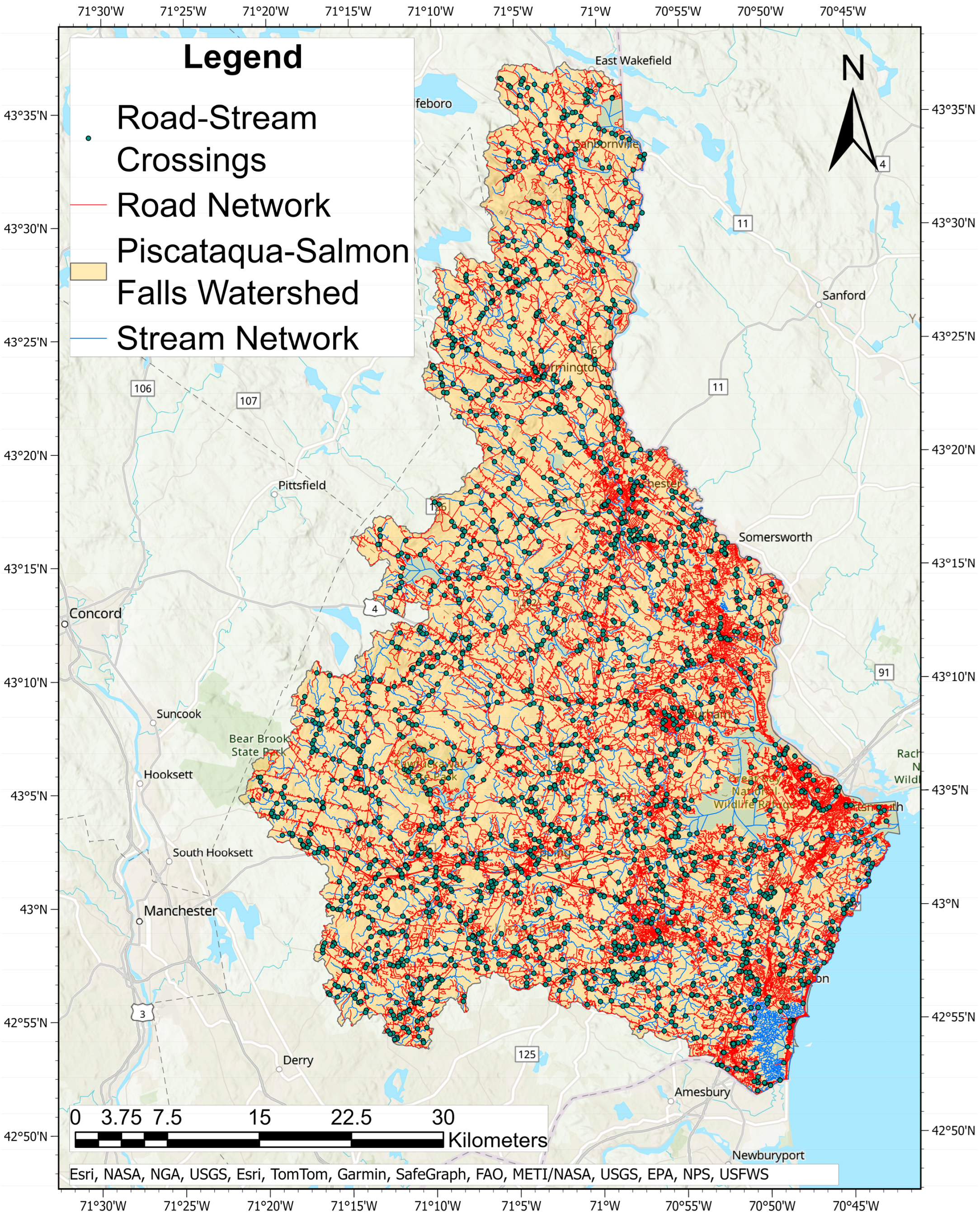
2.1. Study Area: The Piscataqua–Salmon Falls Watershed

The Piscataqua–Salmon Falls watershed spans 1684 square miles across the states of NH, Massachusetts, and Maine. For this study, we focused on the NH portion of the watershed (Figure 1) to ensure consistency in data sources and alignment with agency-specific prioritization schemes. This area contains approximately 2289 known RSCs, which are owned and maintained by different entities depending on their location: the state for crossings on state-owned roads, municipalities for those on local roads, and private individuals or organizations for crossings on private roads [51,52]. The state environmental agency and the state transportation agency are the two main stakeholders in RSC management. We obtained the current RSC prioritization criteria and schemes directly from these agencies.
Of the 2289 RSCs in the watershed, some were excluded from the prioritization analyses for the following reasons. (1) A total of 351 bridge RSCs were excluded, as they are typically managed separately. (2) A total of 378 RSCs without length data were excluded because their management costs cannot be estimated. (3) A total of 203 RSCs without road-tier data were excluded because transportation scores could not be calculated, and most of these are on private roads or off-road trails. (4) Nine ford RSCs, where water flows over the road, were excluded because environmental and transportation scores are not applicable, and they are mostly located on off-road trails. (5) Eleven additional RSCs on private roads were excluded due to missing data. After these exclusions, a total of 1337 RSCs were included in the final analyses.

2.2. Current RSC Prioritization Criteria and Schemes

Below, we describe the calculations of management costs and RSC prioritization criteria, reflecting the interests of state environmental and transportation agencies.

2.2.1. The State Environmental Agency’s RSC Prioritization Criteria

The state environmental agency’s RSC prioritization criteria include the following: aquatic organism passage (AOP), geomorphic compatibility (GC), hydraulic capacity (HC), and structural condition (SC). Data for these criteria were obtained from the NH Statewide Asset Data Exchange System (SADES) [53], which inventories primary data collected through a multi-year, statewide RSC field survey effort led by the NH Stream Crossing Initiative [54].
The average of the four scores was used as the “environmental score”, which ranges from 0 to 1. A higher environmental score indicates greater urgency for replacements and more substantial benefits for stakeholders. Table 1 outlines the metrics, rating categories, and prioritization scores assigned to each criterion.

2.2.2. The State Transportation Agency’s RSC Prioritization Criteria

The state transportation agency prioritizes RSC management based on five main criteria: (1) annual average daily traffic (AADT), (2) road tier, (3) RSC material, (4) RSC size, and (5) RSC SC (Table 2). It is important to note that the scoring within each criterion is not based on equal intervals, with significantly higher scores sometimes assigned to conditions deemed “critical” by the agency. Similarly, the score range varies across different criteria. For each RSC, the transportation score, ranging from 0 to 1, was calculated by summing the scores in Table 2 and normalizing the total by dividing it by the maximum possible score of 91.3. We obtained data for AADT and road tier from the NH Geographically Referenced Analysis and Information Transfer (NH GRANIT) database [58], and data for the material, size, and SC from the SADES [53]. Notably, the SC is a shared criterion between the transportation and environmental agencies; however, it has different numerical ratings, reflecting the distinct priorities of the respective agencies.

2.2.3. Management Cost

In this study, we considered replacement as the primary RSC management activity. We applied Equations (1) and (2) to estimate an RSC’s replacement cost [61,62,63]. A detailed discussion of the cost estimation methodology is provided in the Supplementary Materials (Section S1)
C = W L 500 M 0.9290304 × f  
W = 1.2 × B F W + 0.6096  
where C is the RSC replacement cost in February 2024, measured using the USD value. L is the length of the RSC in meters. M is the cost multiplier for different road tiers: 2 for Tiers 1 and 2, 1.8 for Tier 3, 1.2 for Tier 4, 1 for Tier 5, and 1.1 for Tier 6, reflecting their varying complexities [63]. W is the required width in meters, according to NH standards for RSCs [62]. f is a conversion factor for adjusting the 2018 USD value, which was originally reported by Equation (1), to the February 2024 USD value. It is calculated as the ratio between the February 2024 consumer price index (CPI) of 310.2 and the 2018 average CPI of 251.1 [64]. BFW is the bankfull width in meters. The SADES provided bankfull widths for about 646 RSCs. For the remaining 691 RSCs [53], their bankfull widths were estimated using Equation (3) [61].
B F W = 4.042 D A 2.58999 0.4459  
where DA is each RSC’s upstream drainage area in square kilometers. The upstream drainage area for each RSC is delineated using the ArcPy module within the ArcGIS Pro environment [65] based on the USGS National Hydrography Dataset Plus High Resolution [66].
A cost score ranging from 0 to 1 was then calculated as Replacement   Cost m a x Replacement   Cost . The cost score is normalized in a different way than the environmental and transportation scores because a few RSCs with very high costs will result in a skewed cost score distribution if taking a linear normalization approach. This adjusted normalization approach allows the cost score distribution to resemble those of the environmental and transportation scores.

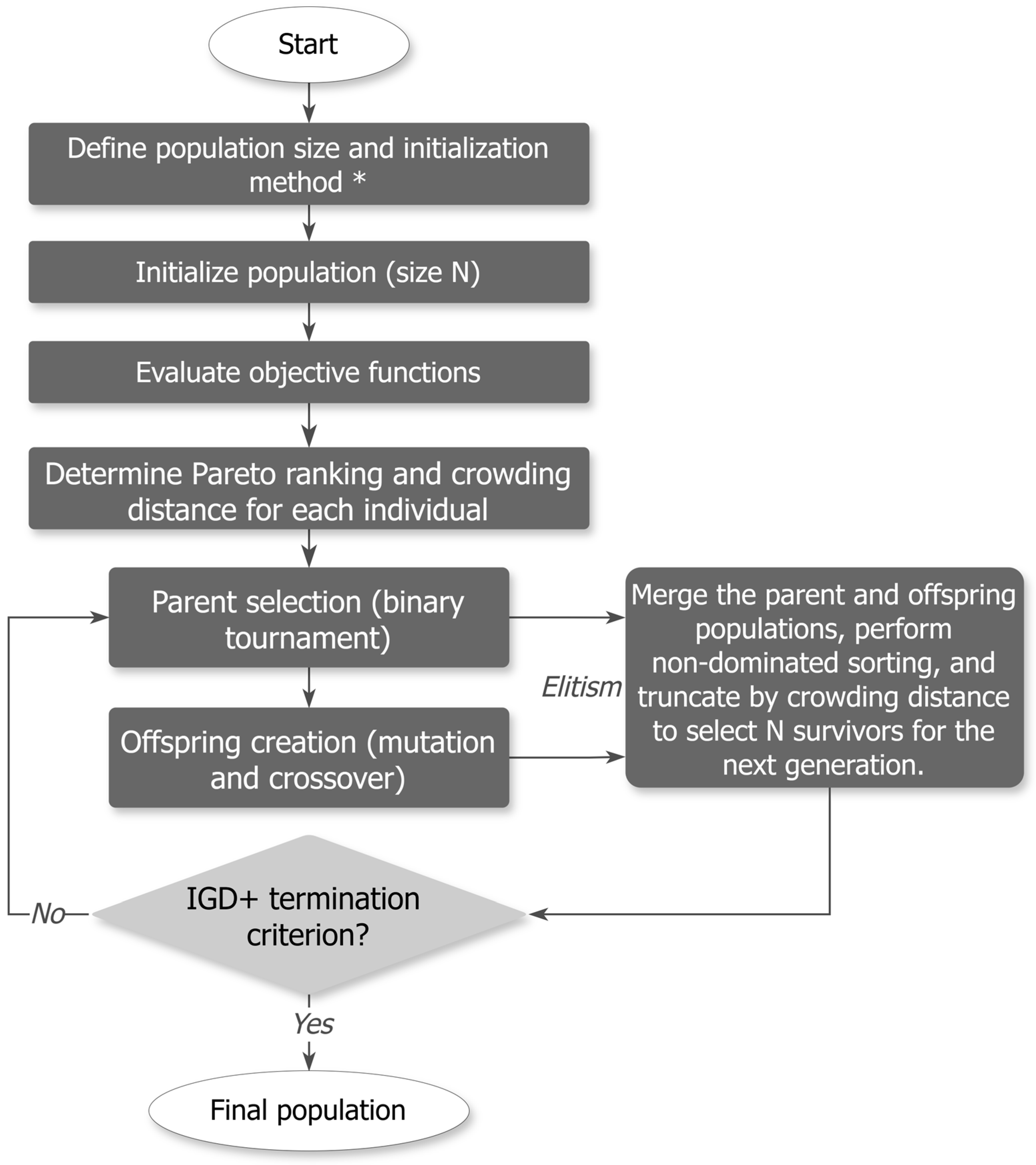
2.3. NSGA-II Multi-Objective Prioritization Framework

Our prioritization framework has the following objective function (Equation (4)):
min X i = 1 N X i S env , i , i = 1 N X i S trans , i , i = 1 N X i S cost , i  
where X = (X1, X2, …Xi, XN) is the binary decision vector, where Xi = 1 means that the i-th RSC is selected for replacement, and Xi = 0 means that it is not selected; N is the number of RSCs in the watershed (1337 in this study); and Senv,i, Strans,i, and Scost,i are the environmental, transportation, and cost scores for the i-th crossing. MOO seeks to identify a set of Pareto-optimal solutions (decision vectors), also known as non-dominated solutions or the Pareto frontier, where no better solution can be found with respect to all three objectives [39]. Given the extensive pool of 21337 possible solutions, the NSGA-II approach was employed to efficiently search for the Pareto frontier.
Beginning with an initial population of replacement decision vectors (i.e., solutions), the NSGA-II algorithm runs in iterations to steer the search toward optimal or near-optimal solutions until a termination criterion is met [67]. Each iteration is referred to as a “generation”. The best-performing solutions from each generation are selected as “parents” to produce “offspring” through processes including crossover and mutation. A key advantage of NSGA-II is its incorporation of elitism, which allows the next generation to be selected from a combined pool of the current population and the newly generated offspring [49]. We implemented the NSGA-II algorithm using version 1.4 of the distributed evolutionary algorithms in Python (DEAP) package [68]. Figure 2 shows the process involved in the NSGA-II framework.
To reduce computational cost and enhance optimization effectiveness, we evaluated various model configurations, including the initialization method and population size. The performance of different model configurations was evaluated using the modified inverted generational distance (IGD+), which measures the distance between an obtained Pareto front and a reference Pareto front approximating the true Pareto front [69]. To approximate the reference Pareto front, we first ran the NSGA-II algorithm with a large population size (20 N = 20 × 1337) to ensure broad coverage of the solution space. A large number of generations was used to ensure convergence to the true Pareto front. This was monitored by using incremental IGD+ between two consecutive Pareto fronts. Further details on the incremental IGD+ methodology are provided in the Supplementary Materials (Section S2).
Once the reference Pareto front was identified, the IGD+ was calculated as the distance between an obtained Pareto front and the identified reference Pareto front. Because different objectives have vastly different value ranges, objectives with larger scales would disproportionately influence the distance metric. To resolve this, normalization of the IGD+ was conducted. The normalization follows the equation x = x min x ref max x ref min x ref   , where x′ is the normalized objective value; x is the original objective value; min(xref) is the minimum value in the reference set; and max(xref) is the maximum value in the reference set. The normalized IGD+ measures the distance on a standardized scale from 0 to 1, providing a consistent interpretation. For instance, a normalized IGD+ of 0.01 means that the current Pareto front is 1% away from the reference front in the normalized space. This allows IGD+ to serve as an unbiased evaluation metric for optimization performance. We used the “pymoo.indicators.igd_plus” function from version 0.6.1.1 of the pymoo library in Python to calculate the IGD+ [70].
We explored the performance of various population sizes (0.5 N, 1 N, 2 N, 4 N, and 8 N, where N is the length of decision vectors) combined with three different initialization methods. The three initialization methods compared are (1) random sampling across the entire search space; (2) stratified sampling, where the search space was divided into 27 bins based on the number of RSCs selected for replacement in each solution (i.e., ≤50, 51–100, 101–150, etc.), and random samples were generated for each bin [71]; (3) custom seeded sampling, which seeds the initial population with potentially “high-quality” solutions near the Pareto front. To identify these potentially “high-quality” solutions, we first defined 927 cost bins, from USD 1 million to USD 927 million (the total replacement cost of all 1337 RSCs), in USD 1 million increments. In each bin, RSCs were ranked by environmental score and sequentially selected until the budget was exhausted, generating one solution per bin. We repeated this process using transportation scores, yielding a pool of 1854 potentially “high-quality” solutions. If the tested initial population size was smaller than 1854, individuals were randomly sampled from this pool; otherwise, all 1854 were included in the initial population, with the remainder filled via stratified sampling, as described above [72]. Once the population size and initialization method were finalized, we performed a grid search for mutation rates (0.001, 0.005, 0.01, and 0.05) and crossover rates (0.6, 0.7, 0.8, and 0.9) based on established ranges [73] to identify their optimal combination.
Once all optimal NSGA-II model parameters were finalized, we compared the performances of the NSGA-II solutions with the conventional S and R solutions under various budget limitations. In the S and R approach, RSCs are ranked based on either their environmental or transportation scores from highest to lowest and selected sequentially until the budget is exhausted. To enable direct comparison with the S and R approach, the Pareto-optimal solutions obtained from NSGA-II were first filtered based on the corresponding budget limits. Within each budget limit, a refined set of Pareto-optimal solutions was then identified with respect to environmental and transportation scores. Since Pareto-optimal solutions are not unique, we compared their range of scores against that obtained from the S and R approach (the solution is unique when using S and R) under each budget constraint.
We also investigated the characteristics of an RSC that may influence its selection for replacement under the NSGA-II approach. We applied Spearman’s rank correlation to analyze the relationship between the RSC characteristics and their frequency of selection for replacement in the Pareto-optimal solutions, reflecting their relative importance. The RSC characteristics selected include SC, HC, material, GC, road tier, AOP, size, and AADT.

3. Results and Discussion

In this section, we first report the results from the selection of key model parameters of the NSGA-II prioritization framework (Section 3.1). The NSGA-II optimized solutions were then compared with those derived from the conventional S and R method (Section 3.2). Section 3.3 presents the outcomes of the correlation analysis, pinpointing the most influential RSC characteristics in their frequency of selection for replacement in the Pareto-optimal solutions.

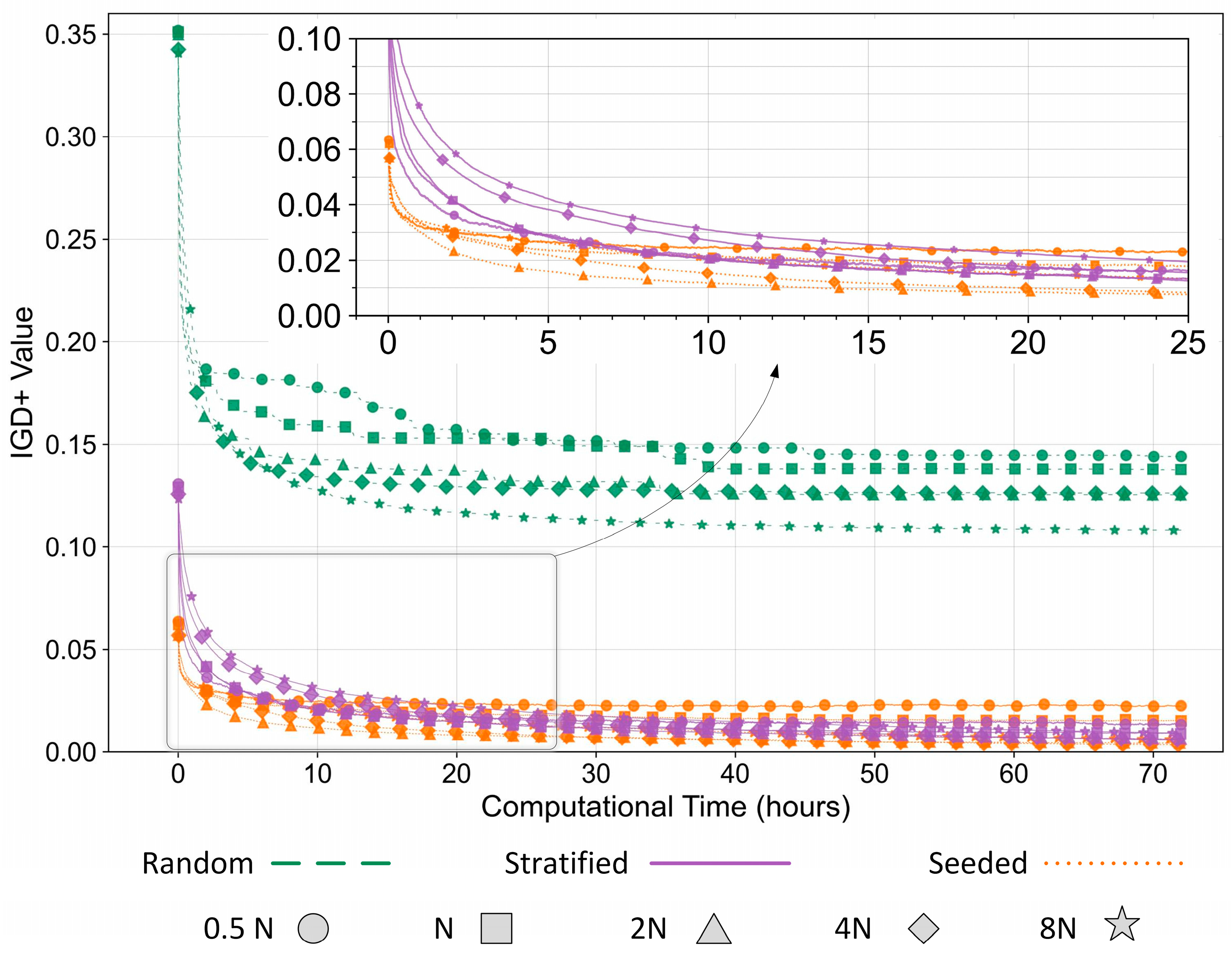
3.1. NSGA-II Prioritization Model Configuration

Figure 3 further presents the performance of the three initialization methods using the selected reference set. Custom seeded initialization was selected as a final initialization method, given its superior coverage and faster convergence. For different population sizes, trade-offs are observed between convergence speed and the solution quality (i.e., the IGD+ value). Smaller populations (0.5 N and N) converge more quickly but stabilize at higher IGD+ values, and vice versa. To obtain a balance between computational efficiency and solution quality, we picked IGD+ = 0.01 as the convergence criterion for algorithm termination, and thereby, a population size of 2 N (2674) was chosen as it leads to the fastest convergence. Similarly, we determined the optimal mutation rate of 0.001 and crossover rate of 0.7 to be used in our final optimization model as they yield the fastest convergence.
Figure 4 presents the Pareto-optimal results obtained from the NSGA-II framework. Figure 4b shows a near-linear relationship between environmental and transportation scores, forming a thin band of Pareto-optimal solutions. This pattern arises from the shared criterion of SC, which influences both objectives and the cost score minimization. Although SC has different ratings across environmental and transportation scores, it can create an inherent positive correlation between environmental and transportation scores. Minimizing cost scores further reinforces this pattern by eliminating extreme solutions that heavily favor one objective over the other, leading to balanced improvements in both environmental and transportation scores.
In contrast, Figure 4c,d reveal a concave Pareto front curve between the environmental and cost scores, as well as between the transportation and cost scores. The knee points in these trade-offs are identified as the solutions with the maximum perpendicular distance to the red dashed line connecting the lowest and highest cost solutions. These turning points represent the solution where further improvements in the objective become disproportionately expensive. Notably, the turning point for transportation occurs at a lower cost (USD 226 million) compared to environmental benefits (USD 283 million), which indicates that transportation benefits are achieved more cost-efficiently under the optimization framework.

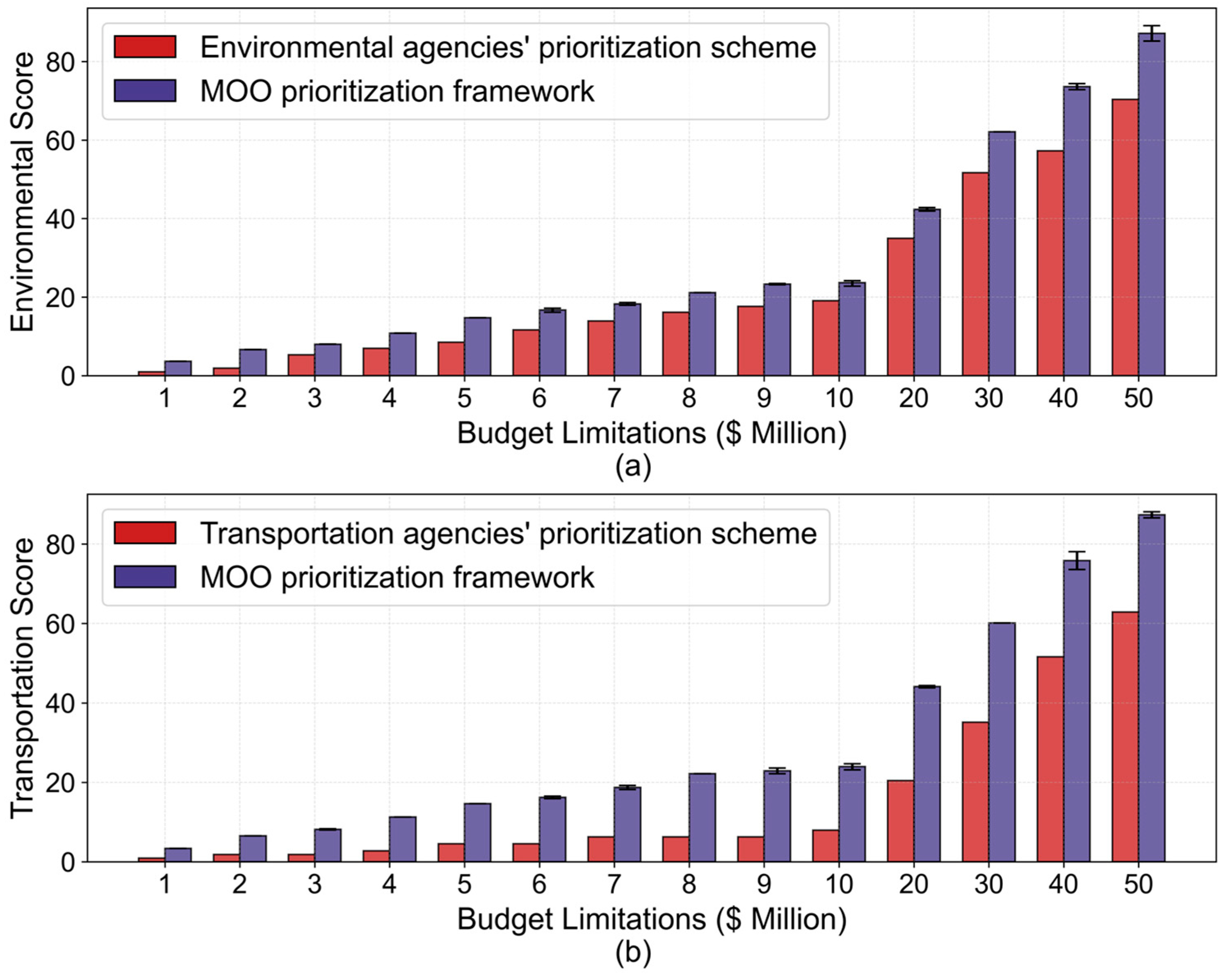
3.2. NSGA-II vs. Conventional Prioritization Schemes

Figure 5 compares the NSGA-II optimization outcome against the conventional S and R approach commonly used by environmental (Figure 5a) and transportation (Figure (b) agencies. The NSGA-II results are presented using bars that show the average scores for each budget scenario, accompanied by error bars that represent the variability within the Pareto-optimal solutions. The narrow range of these scores suggests that the interests of environmental and transportation agencies can be harmonized under a multi-objective optimization approach.
Across all budget levels, the NSGA-II framework consistently outperforms the conventional S and R method for both agencies, with a minimum improvement of 19.56% in environmental score and 37.68% in transportation score. Holding the environmental or transportation score constant, this is equivalent to a cost savings ranging from USD 1.08 million to USD 13.68 million for the environmental agency and from USD 1.49 million to USD 19.87 million for the transportation agency within the USD 50 million budget range. This is because the NSGA-II framework explores various combinations of crossings to maximize overall system-wide benefits within a given budget. The Pareto-optimal solutions may include RSCs with lower individual scores but a higher combined benefit. In contrast, the conventional S and R method ranks RSCs solely based on environmental or transportation scores without considering cost. Its rigid, sequential approach—following a strict descending order of priority—limits the potential for innovative RSC management strategies that, while not always addressing the highest-scoring RSCs first, could ultimately deliver greater overall environmental or transportation benefits. This reveals a conflict between the more direct and intuitive S and R thinking in real-world RSC management practices and the more efficient but potentially less intuitive MOO approach. While the S and R approach may be unavoidable in many practical situations, MOO provides a valuable perspective by revealing a range of alternative options available to decision-makers. As such, a hybrid or adaptive strategy that integrates both the S and R and MOO approaches may help facilitate the transition. Interactive tools for users can help alleviate the cognitive load associated with applying the MOO approach, making the process more intuitive and manageable. It is also important to note that real-world implementation would likely temper achievable savings through MOO due to factors not included in our model, such as permitting administrative overheads and funding uncertainties. Additionally, incorporating factors such as economies of scale, social equity, and system criticality into the MOO analysis can enhance its realism and practical relevance.
It was also found that the benefit margin of the NSGA-II prioritization framework—the difference between the NSGA-II and the S and R scores per USD million budget—decreases as the budget increases. This indicates that the S and R approach could be less efficient under a smaller budget as the selection of high-cost crossings quickly depletes smaller budgets, thereby creating a larger performance gap relative to the NSGA-II approach. As budgets grow, this issue becomes less pronounced, leading to a reduced margin of improvement for NSGA-II. This highlights the importance of incorporating the replacement cost of crossings in decision-making. Stakeholders with very limited budgets (e.g., non-profit organizations) can obtain greater benefits from adopting NSGA-II, as it selects crossings more efficiently under tight financial constraints.
Moreover, the benefit margin of the transportation score is, on average, 123.98% higher than the environmental score. This is because transportation agencies tend to prioritize large crossings located on high-traffic roads with lower road tier values under the current practice. These expensive projects can quickly exhaust a limited budget under the S and R method, yielding lower overall returns. From a policy standpoint, transportation agencies could refine their schemes by making higher scores for size, AADT, and road tier conditional on deteriorated structural conditions so that crossings with adequate structural integrity are not automatically prioritized, thereby fostering more balanced outcomes.

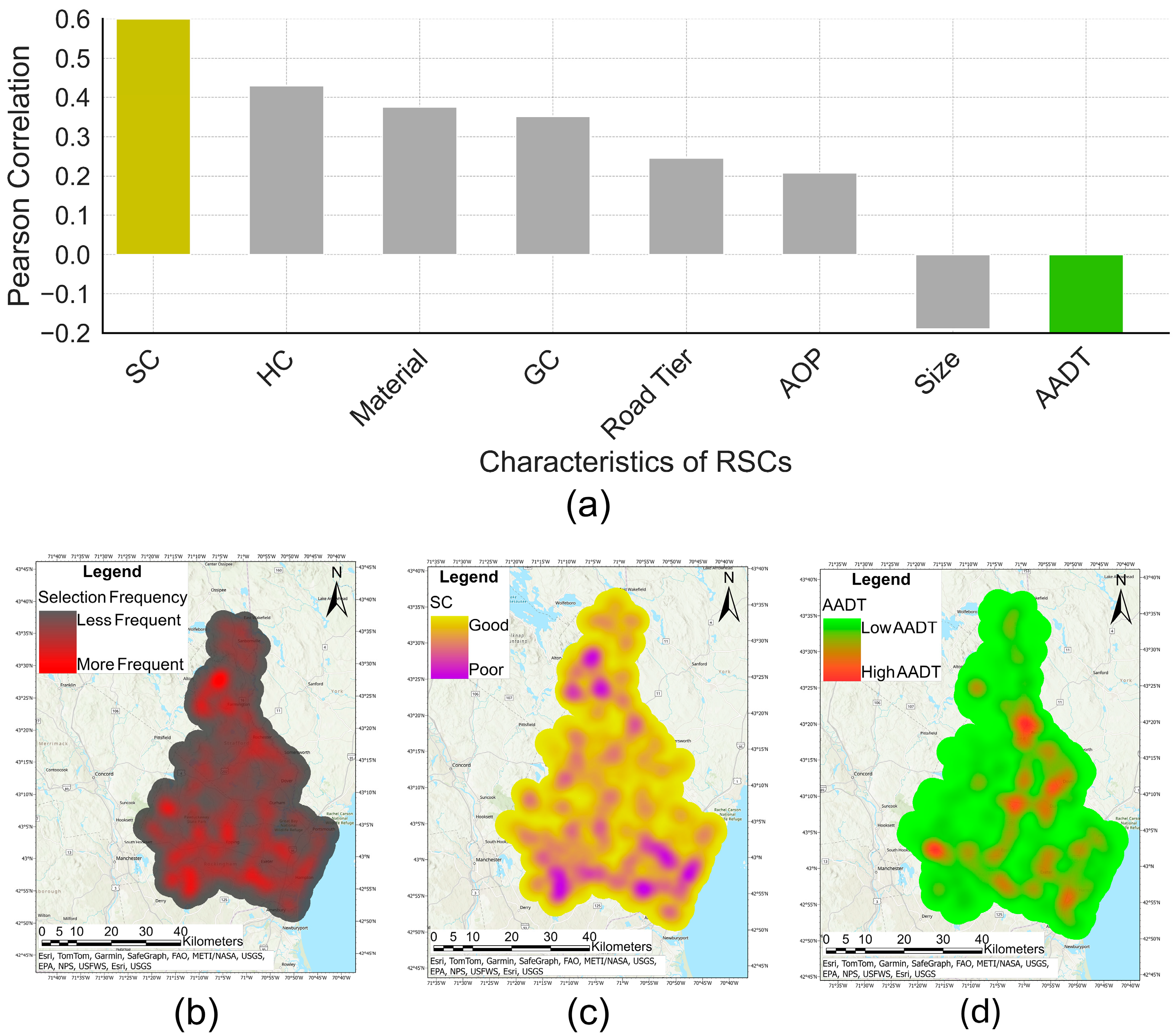
3.3. RSC Characteristics That Influence Their Selection in Optimal Solutions

Figure 6a shows the correlation between various RSC characteristics and the frequency of the RSC being selected in the Pareto-optimal solution set. Among the characteristics, SC exhibits the strongest correlation with the frequency of RSC replacement, followed by HC, material, and GC. In contrast, size and AADT have negative correlations with selection frequency. This may be because larger RSCs on high-traffic roads are less critical for AOP, GC, or HC while also incurring higher replacement costs, making them less likely to be selected in the Pareto-optimal solution set. Our findings suggest that SC plays a pivotal role in prioritizing RSC replacements, as its strong correlation with selection frequency in the NSGA-II framework indicates its ability to balance transportation, environmental, and cost considerations. By contrast, the negative correlation of size and AADT with selection frequency suggests that these factors, although prioritized in the transportation prioritization scheme, do not effectively balance the interests of environmental and transportation agencies when minimizing replacement costs. Overall, these results highlight which characteristics resonate with the balanced approach of NSGA-II and suggest that stakeholders without the capacity to implement complex prioritization models could focus on key aspects such as SC and HC for effective decision-making.
Figure 6b–d provide a side-by-side comparison of the geographical heatmaps for RSC selection frequency, SC, and AADT. The alignment of these heatmaps supports the findings from the correlation analysis. The spatial distribution of frequently selected RSCs reveals that high-priority replacements are scattered across the watershed. This emphasizes the importance of a systematic, watershed-scale prioritization strategy. However, implementing solutions at this scale may face coordination challenges due to differing crossing ownerships, municipal priorities, resource limitations, and decision-making processes. Addressing these challenges requires a collaborative and integrated management approach that aligns local efforts with the broader goals of watershed-wide sustainability. Examples of actionable steps include forming a regional task force to coordinate efforts across municipalities, establishing pooled funding mechanisms to bridge resource gaps, and creating standardized prioritization criteria that balance local needs with regional sustainability objectives.

4. Conclusions

Given the critical role of RSCs in environmental sustainability and transportation safety, this study seeks to develop an NSGA-II MOO framework for RSC management prioritization that maximizes and balances diverse stakeholder interests and minimizes overall management costs. The results were compared to the conventional S and R prioritization scheme. Using an optimized NSGA-II configuration, we found that the NSGA-II approach achieved at least 19.56% higher environmental scores and 37.68% higher transportation scores than conventional S and R schemes under various budget limitations while efficiently balancing environmental and transportation agencies’ interests. These improvements translate to cost savings ranging from USD 1.08 million to USD 19.87 million within a USD 50 million budget limit. The benefit margin of the NSGA-II prioritization framework, however, decreases with increases in the total budget, as the efficiency of the S and R approach increases with a growing budget. This indicates that stakeholders with limited budgets may obtain greater benefits from adopting NSGA-II. Our findings also suggest that SC plays a pivotal role in prioritizing RSC replacements. Its strong correlation with selection frequency among the NSGA-II solutions indicates its ability to balance transportation, environmental, and cost considerations.
Our findings suggest that cost-effective solutions exist that can potentially align the interests of both environmental and transportation agencies. The Pareto-optimal solutions generated by the NSGA-II approach often consist of combinations of multiple RSCs distributed across the watershed, highlighting the need for systematic, watershed-scale prioritization strategies. However, the implementation of such strategies may be hindered by coordination challenges, including differing crossing ownerships, municipal priorities, decision-making processes, and resource constraints. Facilitating meaningful stakeholder engagement across the watershed could serve as a vital step toward consensus-building and fostering cross-jurisdictional collaboration.
While this study focuses on two primary stakeholders in RSC management, the environmental and transportation agencies, future research could incorporate additional stakeholders and their preferences for a more comprehensive analysis. Interpreting NSGA-II results requires a level of systems thinking and data science expertise, making it less intuitive than the traditional S and R approach commonly used in practice. Nevertheless, a hybrid and adaptive pathway that integrates the S and R and MOO approaches may facilitate the transition. Developing a user-friendly online tool could improve accessibility and usability, expanding the applicability of NSGA-II to a broader audience and facilitating more informed decision-making. The methodological framework developed in this study has broad implications for the management of additional types of infrastructure systems with large maintenance needs and diverse stakeholder interests, such as dams [74] and green infrastructure [75]. By embracing these integrated strategies, decision-makers can better balance competing priorities, enhance transparency, and promote sustainable infrastructure planning.

Supplementary Materials

The following supporting information can be downloaded at: https://www.mdpi.com/article/10.3390/su17093987/s1, Section S1. Road–stream crossings cost estimation discussion, Section S2. Monitoring convergence using incremental modified inverted generational distance, Figure S1: Incremental modified inverted generational distance (IGD+) over generations, used as a convergence metric. Incremental IGD+ measures the IGD+ metric between consecutive Pareto fronts, using the next generation’s Pareto front as the reference. Dataset S1: Road-Stream Crossing Optimization Dataset.

Author Contributions

Conceptualization, S.G.R. and W.M.; Data curation, K.A.; Formal analysis, K.A.; Funding acquisition, E.S.B. and W.M.; Investigation, K.A., S.G.R., F.H., and W.M.; Methodology, K.A., S.G.R., F.H., and W.M.; Project administration, W.M.; Resources, F.H., E.S.B., and W.M.; Supervision, F.H. and W.M.; Validation, K.A., F.H., and W.M.; Visualization, K.A. and A.H.T.; Writing—original draft, K.A.; Writing—review and editing, K.A., S.G.R., A.H.T., F.H., E.S.B., and W.M. All authors have read and agreed to the published version of the manuscript.

Funding

This research was funded by the American Rescue Plan Act, administrated via the New Hampshire Department of Environmental Services, grant number VC #315187-B083. The views, findings, and conclusions expressed in this study are those of the authors and do not necessarily reflect the views of the funding agency.

Institutional Review Board Statement

Not applicable.

Informed Consent Statement

Not applicable.

Data Availability Statement

The data presented in this study are publicly available from the following sources: NH GRANIT, NH DOT Roads | New Hampshire Geodata Portal. Available online: https://new-hampshire-geodata-portal-1-nhgranit.hub.arcgis.com/datasets/e8e2c844063f465ba284114cd08d0ecf_18/explore (accessed on 24 February 2022). NH Statewide Asset Data Exchange System (SADES), SADES Stream Crossings. Available online: https://nhdes.maps.arcgis.com/home/item.html?id=c60cb62cb57a46b8a3635d5b98c4e3d4#overview (accessed on 23 February 2024). U.S. Geological Survey (USGS), National Hydrography Dataset Plus High Resolution (NHDPlus HR for HUC 010600—2012). Available online: https://www.usgs.gov/national-hydrography/access-national-hydrography-products (accessed on 6 June 2023). U.S. Bureau of Labor Statistics (BLS), Consumer Price Index for All Urban Consumers (CPI-U). Available online: https://data.bls.gov/timeseries/CUUR0000SA0?years_option=all_years (accessed on 7 April 2024).

Acknowledgments

We thank Polly Crocker, Kevin Lucey, Brian Hauschild, and Matt Urban for sharing current prioritization schemes and interpreting available data.

Conflicts of Interest

The authors declare no conflicts of interest. The funders had no role in the design of the study; in the collection, analyses, or interpretation of data; in the writing of the manuscript; or in the decision to publish the results.

Abbreviations

The following abbreviations are used in this manuscript:
RSCsRoad–Stream Crossings
MOOMulti-Objective Optimization
S and RScoring and Ranking
NSGA-IINon-Dominated Sorting Genetic Algorithm
NHNew Hampshire
AOPAquatic Organism Passage
GCGeomorphic Compatibility
HCHydraulic Capacity
SCStructural Condition
SADESStatewide Asset Data Exchange System
AADTAnnual Average Daily Traffic
IGD+Modified Inverted Generational Distance
CPIConsumer Price Index

References

  1. Roy, S.; Sahu, A.S. Road-Stream Crossing an in-Stream Intervention to Alter Channel Morphology of Headwater Streams: Case Study. Int. J. River Basin Manag. 2018, 16, 1–19. [Google Scholar] [CrossRef]
  2. Wieferich, D.J. Database of Stream Crossings in the United States. In U.S. Geological Survey; U.S. Department of the Interior: Washington, DC, USA, 2022. [Google Scholar] [CrossRef]
  3. Sleight, N.; Neeson, T.M. Opportunities for Collaboration between Infrastructure Agencies and Conservation Groups: Road-Stream Crossings in Oklahoma. Transp. Res. D Transp. Environ. 2018, 63, 622–631. [Google Scholar] [CrossRef]
  4. Southeast Aquatic Resources Partnership Comprehensive Aquatic Barrier Inventory v3.16.0 (02/14/2025). Available online: https://southeastaquatics.net/sarps-programs/aquatic-connectivity-program-act (accessed on 24 February 2025).
  5. Gillespie, N.; Unthank, A.; Campbell, L.; Anderson, P.; Gubernick, R.; Weinhold, M.; Cenderelli, D.; Austin, B.; McKinley, D.; Wells, S.; et al. Flood Effects on Road–Stream Crossing Infrastructure: Economic and Ecological Benefits of Stream Simulation Designs. Fisheries 2014, 39, 62–76. [Google Scholar] [CrossRef]
  6. Hudy, M.; Thieling, T.M.; Gillespie, N.; Smith, E.P. Distribution, Status and Perturbations to Brook Trout within the Eastern United States; Trout Unlimited: Arlington, VA, USA, 2005. [Google Scholar]
  7. Levine, J. An Economic Analysis of Improved Road-Stream Crossings; The Nature Conservancy Adirondack Chapter: Keene Valley, NY, USA, 2013. [Google Scholar]
  8. Perkin, J.S.; Gido, K.B.; Al-Ta’ani, O.; Scoglio, C. Simulating Fish Dispersal in Stream Networks Fragmented by Multiple Road Crossings. Ecol. Modell. 2013, 257, 44–56. [Google Scholar] [CrossRef]
  9. Rieman, B.E.; Lee, D.C.; Thurow, R.F. Distribution, Status, and Likely Future Trends of Bull Trout within the Columbia River and Klamath River Basins. N. Am. J. Fish. Manag. 1997, 17, 1111–1125. [Google Scholar] [CrossRef]
  10. Olson, S.A. Flood of October 8 and 9, 2005, on Cold River in Walpole, Langdon, and Alstead and on Warren Brook in Alstead, New Hampshire. In U.S. Geological Survey; U.S. Department of the Interior: Washington, DC, USA, 2006. [Google Scholar]
  11. Mayo, T.L.; Lin, N. Climate Change Impacts to the Coastal Flood Hazard in the Northeastern United States. Weather Clim. Extrem. 2022, 36, 100453. [Google Scholar] [CrossRef]
  12. Swain, D.L.; Wing, O.E.J.; Bates, P.D.; Done, J.M.; Johnson, K.A.; Cameron, D.R. Increased Flood Exposure Due to Climate Change and Population Growth in the United States. Earths Future 2020, 8, e2020EF001778. [Google Scholar] [CrossRef]
  13. American Society of Civil Engineers 2021 Infrastructure Report Card. Available online: https://infrastructurereportcard.org/cat-item/stormwater-infrastructure/ (accessed on 28 August 2024).
  14. Roy, S.G.; Daigneault, A.; Zydlewski, J.; Truhlar, A.; Smith, S.; Jain, S.; Hart, D. Coordinated River Infrastructure Decisions Improve Net Social-Ecological Benefits. Environ. Res. Lett. 2020, 15, 104054. [Google Scholar] [CrossRef]
  15. New England Environmental Finance Center. A Financial Impact Assessment of LD 1725: Stream Crossings. In Economics and Finance. 5; New England Environmental Finance Center: Portland, ME, USA, 2011. [Google Scholar]
  16. Gautam, S.; Bhattarai, R. Low-Water Crossings: An Overview of Designs Implemented along Rural, Low-Volume Roads. Environments 2018, 5, 22. [Google Scholar] [CrossRef]
  17. Long, J. The Economics of Culvert Replacement: Fish Passage in Eastern Maine. Available online: https://www.climatehubs.usda.gov/sites/default/files/EconomicsOfCulvertReplacement.pdf (accessed on 12 February 2025).
  18. Fuss & O’Neill Order of Magnitude Opinion of Construction Cost for Road-Stream Crossing Replacement. Available online: https://www.southhadley.org/DocumentCenter/View/8566/Culvert-Replacement-Cost-Estimates---May-2021?bidId= (accessed on 12 February 2025).
  19. New Hampshire Department of Environmental Services Funding Opportunities for Stream Crossing Projects. Available online: https://www4.des.state.nh.us/NH-Stream-Crossings/wp-content/uploads/2021/09/FundingTable_Final.pdf (accessed on 27 August 2024).
  20. Throwe, J.; Anderson, B.; Beary, L.; Beecher, J.; Chapman, T.; Chow, R.; Crooks, E.; Daniel, L.; Chu, E.H.; Roberts De La, M.; et al. Evaluating Stormwater Infrastructure Funding and Financing; Environmental Financial Advisory Board Stormwater Infrastructure Finance Task Force; U.S. Environmental Protection Agency: Washington, DC, USA, 2020. [Google Scholar]
  21. McKay, S.K.; Martin, E.H.; McIntyre, P.B.; Milt, A.W.; Moody, A.T.; Neeson, T.M. A Comparison of Approaches for Prioritizing Removal and Repair of Barriers to Stream Connectivity. River Res. Appl. 2020, 36, 1754–1761. [Google Scholar] [CrossRef]
  22. Stack, L.; Simpson, M.H.; Crosslin, T.; Roseen, R.; Sowers, D.; Lawson, C. The Oyster River Culvert Analysis Project; Piscataqua Region Estuaries Partnership: Durham, NH, USA, 2010. [Google Scholar]
  23. Hunt, J.H.; Zerges, S.M.; Roberts, B.C.; Bergendahl, B. CULVERT ASSESSMENT AND DECISION-MAKING PROCEDURES MANUAL For Federal Lands Highway; U.S. Department of Transportation Fedaral Highway Administration: Lakewood, CO, USA, 2010. [Google Scholar]
  24. Diebel, M.W.; Fedora, M.; Cogswell, S.; O’Hanley, J.R. Effects of Road Crossings on Habitat Connectivity for Stream-Resident Fish. River Res. Appl. 2015, 31, 1251–1261. [Google Scholar] [CrossRef]
  25. King, S.; O’Hanley, J.R. Optimal Fish Passage Barrier Removal—Revisited. River Res. Appl. 2016, 32, 418–428. [Google Scholar] [CrossRef]
  26. Konisky, R. Assessment of Road Crossings for Improving Migratory Fish Passage in the Winnicut River Watershed; The Nature Conservancy: Concord, NH, USA, 2009. [Google Scholar]
  27. Neeson, T.M.; Ferris, M.C.; Diebel, M.W.; Doran, P.J.; O’Hanley, J.R.; McIntyre, P.B. Enhancing Ecosystem Restoration Efficiency through Spatial and Temporal Coordination. Proc. Natl. Acad. Sci. USA 2015, 112, 6236–6241. [Google Scholar] [CrossRef]
  28. O’Hanley, J.R.; Wright, J.; Diebel, M.; Fedora, M.A.; Soucy, C.L. Restoring Stream Habitat Connectivity: A Proposed Method for Prioritizing the Removal of Resident Fish Passage Barriers. J. Environ. Manag. 2013, 125, 19–27. [Google Scholar] [CrossRef]
  29. O’Hanley, J.R.; Tomberlin, D. Optimizing the Removal of Small Fish Passage Barriers. Environ. Model. Assess. 2005, 10, 85–98. [Google Scholar] [CrossRef]
  30. Poplar-Jeffers, I.; Petty, T.; Anderson, J.; Kite, J.; Strager, M.; Fortney, R. Culvert Replacement and Stream Habitat Restoration: Implications from Brook Trout Management in an Appalachian Watershed, U.S.A. Restor. Ecol. 2008, 17, 404–413. [Google Scholar] [CrossRef]
  31. Wu, X.; Sheldon, D.; Zilberstein, S. Rounded Dynamic Programming for Tree-Structured Stochastic Network Design. In Proceedings of the AAAI Conference on Artificial Intelligence, Quebec City, QC, Canada, 20 June 2014; Volume 28. [Google Scholar]
  32. Bechtel, D.; Ingraham, P. River Continuity Assessment of the Ashuelot River Basin; The Nature Conservancy. Prepared for New Hampshire Department of Environmental Services, Rivers Management and Protection Program: Concord, NH, USA, 2008. [Google Scholar]
  33. Kurt, C.E.; McNichol, G.W. Microcomputer-Based Culvert Ranking System. Transp Res. Rec. 1335 1991, 21–27. Available online: https://trid.trb.org/view/364810 (accessed on 11 February 2025).
  34. Milone and MacBroom. Piscataquog River Watershed Culvert Prioritization Model; Prepared for Southern New Hampshire Planning Commission; Milone & Macbroom: Piscataquog River Watershed, NH, USA, 2016. [Google Scholar]
  35. Poppenwimer, C.; Kimball, K.D. Priority Connectivity Projects in the Upper Connecticut River Mitigation and Enhancement Fund (MEF) Service Area. Available online: https://www.nhcf.org/wp-content/uploads/2015/12/MEF-Priority-Connectivity-Projects-Report-2016.pdf (accessed on 11 December 2024).
  36. Kemp, P.S.; O’hanley, J.R. Procedures for Evaluating and Prioritising the Removal of Fish Passage Barriers: A Synthesis. Fish. Manag. Ecol. 2010, 17, 297–322. [Google Scholar] [CrossRef]
  37. Lin, H.; Robinson, K.F.; Walter, L. Trade-offs among Road–Stream Crossing Upgrade Prioritizations Based on Connectivity Restoration and Erosion Risk Control. River. Res. Appl. 2020, 36, 371–382. [Google Scholar] [CrossRef]
  38. Emmerich, M.T.M.; Deutz, A.H. A Tutorial on Multiobjective Optimization: Fundamentals and Evolutionary Methods. Nat. Comput. 2018, 17, 585–609. [Google Scholar] [CrossRef]
  39. Gunantara, N. A Review of Multi-Objective Optimization: Methods and Its Applications. Cogent. Eng. 2018, 5, 1502242. [Google Scholar] [CrossRef]
  40. Han, S.-W.; Lee, E.H.; Kim, D.-K. Multi-Objective Optimization for Skip-Stop Strategy Based on Smartcard Data Considering Total Travel Time and Equity. Transport. Res. Rec. 2021, 2675, 841–852. [Google Scholar] [CrossRef]
  41. Eckart, K.; McPhee, Z.; Bolisetti, T. Multiobjective Optimization of Low Impact Development Stormwater Controls. J. Hydrol. 2018, 562, 564–576. [Google Scholar] [CrossRef]
  42. Raseman, W.J.; Kasprzyk, J.R.; Summers, R.S.; Hohner, A.K.; Rosario-Ortiz, F.L. Multi-Objective Optimization of Water Treatment Operations for Disinfection Byproduct Control. Environ. Sci. Water Res. Technol. 2020, 6, 702–714. [Google Scholar] [CrossRef]
  43. Zhang, W.; Cao, K.; Liu, S.; Huang, B. A Multi-Objective Optimization Approach for Health-Care Facility Location-Allocation Problems in Highly Developed Cities Such as Hong Kong. Comput. Environ. Urban Syst. 2016, 59, 220–230. [Google Scholar] [CrossRef]
  44. Rajagopalan, A.; Nagarajan, K.; Bajaj, M.; Uthayakumar, S.; Prokop, L.; Blazek, V. Multi-Objective Energy Management in a Renewable and EV-Integrated Microgrid Using an Iterative Map-Based Self-Adaptive Crystal Structure Algorithm. Sci. Rep. 2024, 14, 15652. [Google Scholar] [CrossRef]
  45. Câmara, D. Evolution and Evolutionary Algorithms. In Bio-Inspired Networking; Elsevier: Amsterdam, The Netherlands, 2015; pp. 1–30. ISBN 978-1-78548-021-8. [Google Scholar]
  46. Galvan, B.; Greiner, D.; Périaux, J.; Sefrioui, M.; Winter, G. Parallel Evolutionary Computation for Solving Complex CFD Optimization Problems: A Review and Some Nozzle Applications. In Parallel Computational Fluid Dynamics 2002; Elsevier: Amsterdam, The Netherlands, 2003; pp. 573–604. ISBN 978-0-444-50680-1. [Google Scholar]
  47. Monteiro, A.C.B.; França, R.P.; Arthur, R.; Iano, Y. 2—The Fundamentals and Potential of Heuristics and Metaheuristics for Multiobjective Combinatorial Optimization Problems and Solution Methods. In Multi-Objective Combinatorial Optimization Problems and Solution Methods; Toloo, M., Talatahari, S., Rahimi, I., Eds.; Academic Press: Cambridge, MA, USA, 2022; pp. 9–29. ISBN 978-0-12-823799-1. [Google Scholar]
  48. Cerf, S.; Doerr, B.; Hebras, B.; Kahane, Y.; Wietheger, S. The First Proven Performance Guarantees for the Non-Dominated Sorting Genetic Algorithm II (NSGA-II) on a Combinatorial Optimization Problem. In Proceedings of the Thirty-Second International Joint Conference on Artificial Intelligence (IJCAI-23), Macao, China, 19–25 August 2023; International Joint Conferences on Artificial Intelligence Organization: Macau, China, 2023; pp. 5522–5530. [Google Scholar]
  49. Deb, K.; Pratap, A.; Agarwal, S.; Meyarivan, T. A Fast and Elitist Multiobjective Genetic Algorithm: NSGA-II. IEEE Trans. Evol. Comput. 2002, 6, 182–197. [Google Scholar] [CrossRef]
  50. Kollat, J.B.; Reed, P.M. Comparing State-of-the-Art Evolutionary Multi-Objective Algorithms for Long-Term Groundwater Monitoring Design. Adv. Water Resour. 2006, 29, 792–807. [Google Scholar] [CrossRef]
  51. RSA 236:13; Driveways and Access to the Public Way. New Hampshire General Court: Concord, NH, USA, 2024.
  52. Urban, M. Best Management Practices for Routine Roadway Maintenance Activities in New Hampshire; New Hampshire Department of Environmental Services and the New Hampshire Department of Transportation. 2019. Available online: https://mm.nh.gov/files/uploads/dot/remote-docs/best-management-practices-for-routine-roadway-maint-activities.pdf (accessed on 11 February 2025).
  53. NH Statewide Asset Data Exchange System (SADES) Stream Crossings. Available online: https://nhdes.maps.arcgis.com/home/item.html?id=c60cb62cb57a46b8a3635d5b98c4e3d4#overview (accessed on 23 February 2024).
  54. New Hampshire Stream Crossing Initiative. Available online: https://www4.des.state.nh.us/NH-Stream-Crossings/ (accessed on 7 April 2025).
  55. New Hampshire Geological Survey; New Hampshire Department of Environmental Services. Stream Crossing Assessment Initiative Geomorphic and Aquatic Organism Passage Screening Tool Summary. Available online: https://www.des.nh.gov/sites/g/files/ehbemt341/files/documents/2020-01/lrm-geomorphic-aop-screening-tool-summary.pdf (accessed on 30 January 2024).
  56. Ballestero, J.; Ballestero, T. Streamworks Culvert Assessment Model: Version 2 User’s Manual. Available online: https://www.nhcaw.org/wp-content/uploads/2017/06/c-rise-streamworks-users-manual-v2-2017.pdf (accessed on 27 February 2025).
  57. New Hampshire Stream Crossing Initiative New Hampshire Stream Crossing Initiative Field Manual for the Statewide Asset Data Exchange System (SADES). Available online: https://www.des.nh.gov/sites/g/files/ehbemt341/files/documents/co-20-04.pdf (accessed on 31 January 2024).
  58. NH GRANIT NH DOT Roads | New Hampshire Geodata Portal. Available online: https://new-hampshire-geodata-portal-1-nhgranit.hub.arcgis.com/datasets/e8e2c844063f465ba284114cd08d0ecf_18/explore (accessed on 24 February 2022).
  59. Mendi, V.; Srinivasula Reddy, I. Forecasting Future Traffic Trend by Short-Term Continuous Observation. In Proceedings of the IOP Conference Series: Materials Science and Engineering, Bhimavaram, India, 1 December 2020; Volume 1006, p. 012028. [Google Scholar]
  60. Cass, W. NHDOT Highway Tiers—Definitions. Available online: https://mm.nh.gov/files/uploads/dot/remote-docs/final-definitions-tiers.pdf (accessed on 31 January 2024).
  61. Bent, G.C. Equations for Estimating Bankfull-Channel Geometry and Discharge for Streams in the Northeastern United States. In Proceedings of the Joint Federal Interagency Conference, Book of Abstracts, 3rd Federal Interagency Hydrologic Modeling Conference and 8th Federal Interagency Sedimentation Conference, Reno, NV, USA, 2–6 April 2006; p. 314. [Google Scholar]
  62. University of New Hampshire. New Hampshire Stream Crossing Guidelines. Available online: https://www.des.nh.gov/sites/g/files/ehbemt341/files/documents/2020-01/lrm-unh-stream-crossing.pdf (accessed on 17 April 2024).
  63. New Hampshire Department of Transportation Bridge Program Recommended Network Funding. Available online: https://mm.nh.gov/files/uploads/dot/remote-docs/bridge-program-recommended-network-funding.pdf (accessed on 3 February 2024).
  64. U.S. Bureau of Labor Statistics. Consumer Price Index for All Urban Consumers (CPI-U). Available online: https://data.bls.gov/timeseries/CUUR0000SA0?years_option=all_years (accessed on 7 April 2024).
  65. Esri ArcGIS Pro (ArcPy Module) (Version 3.1). Available online: https://pro.arcgis.com/en/pro-app/latest/arcpy/get-started/arcpy-modules.htm (accessed on 11 February 2025).
  66. U.S. Geological Survey National Hydrography Dataset Plus High Resolution (NHDPlus HR for HUC 010600-2012). Available online: https://www.usgs.gov/national-hydrography/access-national-hydrography-products (accessed on 6 June 2023).
  67. Holland, J.H. Genetic Algorithms. Sci. Am. 1992, 267, 66–73. [Google Scholar] [CrossRef]
  68. Fortin, F.-A.; Rainville, F.-M.D.; Gardner, M.-A.; Parizeau, M.; Gagné, C. DEAP: Evolutionary Algorithms Made Easy. J. Mach. Learn. Res. 2012, 13, 2171–2175. [Google Scholar]
  69. Ishibuchi, H.; Masuda, H.; Tanigaki, Y.; Nojima, Y. Modified Distance Calculation in Generational Distance and Inverted Generational Distance. In Evolutionary Multi-Criterion Optimization; Gaspar-Cunha, A., Henggeler Antunes, C., Coello, C.C., Eds.; Lecture Notes in Computer Science; Springer: Cham, Switzerland, 2015; Volume 9019, pp. 110–125. ISBN 978-3-319-15891-4. [Google Scholar]
  70. Blank, J.; Deb, K. Pymoo: Multi-Objective Optimization in Python. IEEE Access 2020, 8, 89497–89509. [Google Scholar] [CrossRef]
  71. Arnab, R. Stratified Sampling. In Survey Sampling Theory and Applications; Elsevier: Amsterdam, The Netherlands, 2017; pp. 213–256. ISBN 978-0-12-811848-1. [Google Scholar]
  72. Friedrich, T.; Wagner, M. Seeding the Initial Population of Multi-Objective Evolutionary Algorithms: A Computational Study. Appl. Soft Comput. 2015, 33, 223–230. [Google Scholar] [CrossRef]
  73. Yang, X.-S. Chapter 2—Analysis of Algorithms. In Nature-Inspired Optimization Algorithms; Yang, X.-S., Ed.; Elsevier: Oxford, UK, 2014; pp. 23–44. ISBN 978-0-12-416743-8. [Google Scholar]
  74. Roy, S.G.; Uchida, E.; De Souza, S.P.; Blachly, B.; Fox, E.; Gardner, K.; Gold, A.J.; Jansujwicz, J.; Klein, S.; McGreavy, B.; et al. A Multiscale Approach to Balance Trade-Offs among Dam Infrastructure, River Restoration, and Cost. Proc. Natl. Acad. Sci. USA 2018, 115, 12069–12074. [Google Scholar] [CrossRef] [PubMed]
  75. Piscopo, A.N.; Weaver, C.P.; Detenbeck, N.E. Using Multiobjective Optimization to Inform Green Infrastructure Decisions as Part of Robust Integrated Water Resources Management Plans. J. Water Resour. Plann. Manage. 2021, 147, 04021025. [Google Scholar] [CrossRef] [PubMed]
Figure 1. The New Hampshire portion of the Piscataqua–Salmon Falls watershed, located in the state’s coastal region, contains approximately 2300 road–stream crossings. Blue and red lines represent rivers and roads, respectively, and green points represent road–stream crossings.
Sustainability 17 03987 g001
Figure 2. Flowchart of the non-dominated sorting genetic algorithm (NSGA-II)’s prioritization framework for road–stream crossing (RSC) prioritization. N is the length of the binary decision vector equal to the number of RSCs. The modified inverted generational distance (IGD+) is utilized to evaluate convergence. * We compared framework results for random, stratified, and custom seeded initialization methods and population sizes of 0.5 N, N, 2 N, 4 N, and 8 N.
Sustainability 17 03987 g002
Figure 3. The performance of various model configurations. Line style denotes different initialization methods: random (dashed), stratified (solid), and seeded (dotted). Marker shape denotes population size: 0.5 N (○), 1 N (□), 2 N (△), 4 N (◇), and 8 N (☆), where N is the number of RSCs. IGD+ (modified inverted generational distance) values on the vertical axis indicate the normalized distance from the reference solution set (approximately true optimal) to the Pareto solution set obtained from each model configuration. The horizontal axis represents hours of computation.
Sustainability 17 03987 g003
Figure 4. The Pareto-optimal solution sets obtained from the non-dominated sorting genetic algorithm prioritization framework. (a) 3D graph for transportation, environmental, and cost scores. (bd) Different 2D projections of the 3D graph.
Sustainability 17 03987 g004
Figure 5. Outcomes of the non-dominated sorting genetic algorithm prioritization framework compared against the conventional prioritization schemes. (a) Results for the environmental agency and (b) results for the transportation agency. Error bars represent the range of the Pareto-optimal solutions corresponding to each budget scenario.
Sustainability 17 03987 g005
Figure 6. Correlation between road–stream crossing (RSC) characteristics and the selection frequency, defined as the number of times each RSC is chosen for replacement among Pareto-optimal solutions obtained from the non-dominated sorting genetic algorithm prioritization framework: (a) Pearson correlation between the selection frequency and characteristics of RSCs; (b) distribution of the selection frequency; (c) distribution of RSC structural conditions; and, (d) distribution of annual average daily traffic (AADT).
Sustainability 17 03987 g006
Table 1. Metrics, ratings, and prioritization scores for environmental criteria.
CriterionDescriptionRatingsPrioritization Scores
Aquatic Organism Passage (AOP)AOP assesses the capacity of RSCs to facilitate the downstream and upstream migration of aquatic organisms. It is determined by the vertical elevation difference at the outlet (outlet drop), presence and depth of the downstream pool, water depth at the outlet, number of culverts at the crossing, outlet invert type, presence of sediment throughout the structure, partial obstruction, and presence of screening at the inlet and outlet [55].Full Passage, No Score—Not Surveyable a0
Reduced Passage0.33
Passage Only for Adult Trout0.66
No Passage1
Geomorphic Compatibility (GC)GC evaluates how well an RSC aligns with the natural geomorphology and hydrological flow of the stream and provides insights into stream and infrastructure health by assessing erosion metrics that affect water quality and width ratios that indicate flood vulnerability [55]. It considers erosion, sediment continuity, structure width ratios, and slope.Fully Compatible, N/A Score b0
Mostly Compatible0.25
Partially Compatible0.5
Fully Incompatible0.75
Mostly Incompatible1
Hydraulic Capacity (HC)HC evaluates an RSC’s ability to transport water during storm events using hydraulic equations and streamflow predictions. HC scores have been calculated for flood recurrence intervals of 10, 25, 50, and 100 years based on RSC field surveys. We used the average of HC scores for all four flood recurrence intervals. HC ratings are based on the shape, material, dimensions, slope, and relative elevation of the crossing to the road surface, as well as watershed characteristics such as drainage area, land cover, soil type, and precipitation [56].Pass, No Rating—Road Elevation c, No Rating—Wide Span c, No Rating c0
Vulnerable0.5
Overtop1
Structural Condition (SC)The SC score assesses the physical state and structural integrity of an RSC. It is based on a visual inspection of the interior walls, surfaces, bottom, wingwalls, and headwalls [57].Good0
Fair0.5
Poor1
a These are generally tidal or wetland crossings that do not typically have an AOP concern [53]. b The “N/A Score” ratings indicate that the waterbody is not a stream, making GC inapplicable [53]. c “No Rating–Road Elevation” indicates that the distance between the road surface and the RSC’s structure cannot be measured, and “No Rating–Wide Span” signifies that the crossing has a wide span [53]. HC cannot be assessed for non-stream waterbodies, such as wetlands, tidal waters, and surface waters. In these cases, as well as the “No Rating” categories, we assigned an HC prioritization score of 0 due to their lower flooding risk.
Table 2. Definitions and scores for transportation criteria.
CriterionDefinitionStatusScore
Annual Average Daily Traffic (AADT)The average number of vehicles passing a specific point on a highway or road per day over a year [59].>20,00010.1
10,000–20,0007.9
6000–10,0005
4000–60003
2000–40002
<20001
Road TierRoad tiers are based on the road’s function and significance. Tier 1 consists of Interstates, Turnpikes, and Divided Highways. Tier 2 includes Statewide Corridors. Tier 3 covers Regional Corridors. Tier 4 is made up of Local Connectors. Finally, Tier 5 comprises Local Roads [60].Tier 15
Tier 24
Tier 33
Tier 42
Tier 51
MaterialThe material used in RSC construction. It can include concrete, metal, plastic, etc.Metal11.3
Masonry6
Concrete1
Plastic0.5
Other5
N/A4
SizeRefers to the span (width) of the RSC, measured at the inlet opening.>60″24.9
36″–54″16.6
24″–30″10.3
<24″0
Structural Condition The physical state and structural integrity of an RSC.Poor40
Fair4
Good0
No rating2
Disclaimer/Publisher’s Note: The statements, opinions and data contained in all publications are solely those of the individual author(s) and contributor(s) and not of MDPI and/or the editor(s). MDPI and/or the editor(s) disclaim responsibility for any injury to people or property resulting from any ideas, methods, instructions or products referred to in the content.

