Abstract
Soil organic carbon (SOC) plays a crucial role in the terrestrial carbon cycle and climate regulation. Quantifying the sensitivity of SOC to climate change is essential for developing effective strategies to address climate change and optimizing agricultural production. This study compares the performance of four machine learning models in assessing SOC, ultimately selecting the optimal Extreme Gradient Boosting model for spatial predictions of surface SOC (0–30 cm) across the country. The results indicate that areas with higher organic carbon density are primarily concentrated in the Tibetan Plateau and northeastern regions. Notably, regions with high uncertainty in predictions correspond to areas of elevated organic carbon density. Average temperature, average precipitation, and the Normalized Difference Vegetation Index were identified as the most influential factors across all models. Based on the predictions from the optimal model and a bottom-up framework, various potential climate change scenarios were considered, allowing for the quantification of SOC sensitivity to climate change. Under scenarios of increased temperatures and decreased precipitation, SOC loss intensified, hindering SOC accumulation. When the average temperature rose by 1.45 °C and precipitation decreased by 14.67%, a loss of 10% in SOC was projected for most regions of China. These findings provide critical insights for the proactive formulation of climate adaptation strategies, soil health preservation, and the maintenance of ecosystem stability.
1. Introduction
Soil organic carbon (SOC) is a crucial component of soil, playing a vital role in the global carbon cycle and climate regulation [1,2]. As the largest carbon reservoir within terrestrial ecosystems, SOC stores approximately twice the amount of carbon found in the atmosphere, highlighting its significant carbon sequestration potential [3,4]. Even minor fluctuations in SOC can influence atmospheric CO2 concentrations and carbon balance, thereby profoundly affecting ecosystem stability. Climate conditions are a key determinant of SOC dynamics, particularly under warming scenarios, which may enhance microbial activity in soils and accelerate the decomposition and cycling of SOC [5]. However, the sensitivity of SOC to climate change varies across different regions [6]. Therefore, a comprehensive understanding of the spatial distribution characteristics of SOC and its response to climate change is essential for assessing the impacts of climate change on ecosystems and for formulating effective environmental management strategies.
Traditional soil mapping relies on soil experts’ accumulated experience and the assistance of geological and topographical maps [7]. However, there are some limitations to this approach, including low temporal resolution, poor spatial resolution, and high costs. The mapping process is cumbersome and time-consuming, and the latest information on SOC is not available in time. The low spatial resolution of the maps does not provide detailed information on SOC distribution. At the same time, the lack of relevant information and high cost also limit the application of traditional soil mapping. In recent years, with the development of information technology and remote sensing, Digital Soil Mapping (DSM) technology has emerged, which utilizes spatial analysis, data mining, and information processing techniques to efficiently and accurately obtain the spatial distribution of soil information; therefore, it has received extensive attention and research. Compared with traditional soil mapping, DSM technology has higher efficiency, more accurate results, and more economical cost; thus, it has become one of the hot spots of current research [8]. It takes the soil-landscape model as its theoretical basis, utilizes soil type and geo-environmental data with synergistic spatial variations, and combines a variety of spatial analysis and statistical means to speculate on the spatial distribution of soils, thus realizing the rapid mapping of soil types. DSM is widely recognized as an effective means to help us update soil data and improve the efficiency of soil information acquisition [2,9].
Machine learning methods can utilize extensive soil samples and environmental variable data to construct high-precision spatial prediction models for SOC [10,11]. Compared to traditional statistical methods, machine learning approaches demonstrate significant advantages in SOC mapping [12,13]. Their core strengths are manifested in three aspects: First, by processing high-dimensional data (such as multispectral remote sensing, terrain-derived variables, and climate data), machine learning can significantly improve the spatial resolution and prediction accuracy of mapping. Second, the algorithms can autonomously identify complex nonlinear relationships between SOC and environmental factors without requiring predefined parametric forms. Furthermore, models based on ensemble learning or Bayesian frameworks (e.g., random forests, Gaussian process regression) can simultaneously output spatial distributions of prediction uncertainty, providing decision-makers with reliability assessment references [14].
In the past 30 years, predictive SOC has made rapid developments. Scholars at home and abroad have carried out a lot of research on acquiring data on environmental variables, sampling methods, and mapping models, and the scale of application has expanded from small-scale to large regions and has even reached the global scale [15]. These advances have significantly improved the accuracy and utility of the spatial distribution estimation of SOC. However, some challenges remain. The first challenge is how to make effective use of new types of data and historical legacy data. Second, model selection and parameter tuning are also a challenge that directly affects the model performance. In addition, the efficiency of different machine learning models in predicting SOC can vary, especially for high-resolution, large-scale regions [16]. In addition to predicting SOC, numerous researchers have employed traditional forward modeling approaches to elucidate the changes in SOC under climate change. For instance, Geremew, et al. [17] and Li, et al. [5] utilized process-based models to forecast trends in SOC across various future scenarios, while Zhou, et al. [18] and Padarian, et al. [19] applied machine learning models to predict alterations in SOC concentration. However, due to significant uncertainties in climate projections and challenges associated with the parameterization of key processes within these models [20,21], such predictions do not always provide effective support for the formulation of management policies. A goal-oriented inverse analysis method capable of exploring SOC dynamics and their sensitivity to climate change without relying on a decision framework of specific future climate projections, also known as the bottom-up approach, has been applied [19,22]. Compared to the traditional top-down approach’s reliance on future scenarios and the limited sufficiency of manual parameter tuning, the bottom-up approach has demonstrated significant advantages in circumventing climate prediction uncertainties, solving parameter optimization challenges, and maintaining scale consistency through the technological paths of spatial gradient substitution, data-driven parameter constraints, and integrated modeling [23,24].
The overarching objective of this study is to evaluate and compare four prominent predictive machine learning algForithms for modeling and forecasting SOC. We assessed their performance differences across large-scale regions in China. Subsequently, based on the optimal model identified, we quantified SOC during the period from 2004 to 2014. Finally, we explored the sensitivity of SOC to climate change over extensive spatial and temporal scales using a bottom-up approach [19], providing a scientific foundation for the development of SOC management strategies and conservation efforts.
2. Materials and Methods
2.1. SOC Data
The SOC density (SOCD) data used in this study were obtained from the 2010s Chinese Terrestrial Ecosystem Carbon Density Dataset compiled by Xu Li [25]. The dataset consists of the following two parts: one part is officially published literature data and the other part is experimental data for the subject group. SOC data recorded 7683 entries, including 4536 SOC entries ranging 0–20 cm in depth (4356 and 180 entries for literature data and experimental monitoring data, respectively). Each data record details the ecosystem type of the sample site, the location of the sample site (longitude and latitude), SOCD (kg m−2), sampling time, data type, and data source. The sources of organic carbon density in soil can be divided into two categories, direct data and indirect data. Direct data refer to carbon density data provided by experimental tests or the literature or SOC data calculated by relevant parameters without conversion or derivation. Indirect data refer to carbon density data that are not provided in experiments or the literature, and the information on related parameters is incomplete and is obtained by further derivation [25].
2.2. Environmental Covariates
The Digital Elevation Model (DEM) is a 1 km resolution dataset based on 1:250,000 contour and elevation point data in China (https://www.geodata.cn). The dataset contains DEM, hillshade, slope, and aspect data. The principle of DEM is to divide the watershed into m rows and n columns of quadrilateral cells, calculate the average elevation of each cell, and store the elevation information in the form of a two-dimensional matrix. With the DEM data, surface morphology information such as slope, slope direction, and the relationship between cells of the watershed grid cells can be extracted. The dataset adopts two projection methods, ortho-axis cut conical equal area projection (Albers Conical Equal Area) and the geodetic coordinate WGS84 coordinate system. DEM is the source data for extracting the topographic factors, and the topographic parameters such as surface elevation, slope, and slope direction can be obtained from the DEM data. These terrain parameters have an important influence on the distribution of SOC. For example, slope and slope direction have an important effect on the distribution of water and the formation of runoff channels, which in turn affects the distribution of SOC and is also an important influence on the accuracy of SOC mapping. In this study, System for Automated Geoscientific Analyses (SAGA) GIS v7.6.3 (https://sourceforge.net/projects/saga-gis/, accessed on 3 August 2024) was used to extract 14 other elevation-derived variables. These include slope, aspect, plan curvature, profile curvature, convergence index, relative slope position, RSP, LS -Factor (LS-Factor, LS), analytical hillshading (AH), closed depressions (CD), total catchment area (TCA), topographic wetness index (TWI), channel network base level (CNB), and channel network distance (CND) (Table 1).

Table 1.
Topographically derived variables.
The precipitation data and temperature data used are the month-by-month precipitation data (Pre) and month-by-month climate data (Tmp) of China on the Spatio-Temporal Tripolar Environmental Big Data platform (https://data.tpdc.ac.cn), which is about 1 km × 1 km, with a time range of 1901.1–2021.12, a unit of precipitation of 0.1 mm, and a unit of temperature of 0.1 °C. The precipitation and temperature data are generated by the Delta Spatial Downscaling Program. This dataset was generated by the Delta spatial downscaling scheme in the Chinese region based on the global 0.5° climate dataset released by CRU and the global high-resolution climate dataset released by WorldClim. Moreover, the data were validated using 496 independent meteorological observation points, and the results were verified to be credible. The format of the data is NETCDF, which was obtained by processing the data into raster format in MATLAB R2023a software and calculating the average year by year to obtain the average value for the period from 2004 to 2014, as well as calculating the precipitation and temperature slopes to obtain the precipitation slope variable (Pre_xl) and the climate slope variable (Tmp_xl).
Potential evapotranspiration (PET) was obtained using the China month-by-month potential evapotranspiration dataset with a spatial resolution of about 1 km and a time period of 1901.1–2022.12 in units of 0.1 mm (https://data.tpdc.ac.cn), which was based on the China 1 km month-by-month mean, minimum, and maximum temperature datasets using the Hargreaves potential evapotranspiration formula. The formula is as follows: PET = 0.0023 × S0 × sqrt (MaxT–MinT) × (MeanT + 17.8), where PET is the potential evapotranspiration, mm/month; MaxT, MinT, and MeanT are the monthly maximum, minimum, and mean temperatures, respectively; and S0 is the theoretical solar radiation that reaches the top of the earth’s atmosphere according to the solar constant, sun–Earth distance, Julian day, and equinox latitude. We selected the data in the time range of 2004.1–2014.12 and averaged them year by year to obtain the average value for the period from 2004 to 2014.
Additionally, we incorporated China’s 1 km annual aridity index dataset (AI) (https://data.tpdc.ac.cn), which was calculated as the ratio of annual precipitation to potential evapotranspiration (Pre/PET). This index, ranging from 0 (hyper-arid) to > 1 (humid), provides a comprehensive moisture availability indicator. All datasets were uniformly processed to obtain 2004–2014 averages, ensuring temporal and spatial consistency across our climate variable analyses.
The normalized difference vegetation index (NDVI) can accurately reflect the surface vegetation cover. The spatial distribution of China’s quarterly 1 km resolution vegetation index (NDVI) dataset is based on the SPOT/VEGETATION PROBA-V 1 KM PRODUCTS (http://www.vito-eodata.be) decadal 1 km vegetation index data, and the quarterly vegetation index dataset since 1998 is generated by using the maximum synthesis method on the basis of the monthly data. The quarterly vegetation index dataset was generated on the basis of monthly data using the maximum value synthesis method since the year 1998. This dataset effectively reflects the distribution and change of vegetation cover in all regions of China in space and time scales, which is of great importance for monitoring the change of vegetation, the rational utilization of vegetation resources, and other ecological environment related fields. The quarterly NDVI data are divided into four quarters: spring (March–May), summer (June–August), fall (September–November), and winter (December–February), and the quarterly NDVI data are the maximum of the NDVI data of the three months in each quarter.
The data acquisition period is from spring 1998 to spring 2020. In this study, the national 1 km resolution month-by-month net primary production (NPP) dataset from 1985–2015 was used to calculate the annual average NPP from 2004 to 2014 using month-by-month averaging (https://www.geodata.cn).
The temperature vegetation dryness index (TVDI) is a soil moisture inversion model constructed based on the NDVI and land surface temperature (LST), and it is particularly suitable for regional drought monitoring and assessing relative dryness during specific time periods within a given year. The global TVDI data used in this study were obtained from the Institute of Geographic Sciences and Natural Resources Research, Chinese Academy of Sciences (http://www.gisrs.cn/), covering the period from 2004 to 2014 with a spatial resolution of 0.0089 degrees (approximately 1 km2). The dataset contains monthly global observations, from which we derived multi-year averages for 2004–2014 through annual averaging processing.
Soil data from 2004 to 2014 were obtained using 2010s data on soil clay (Clay, g kg−1), sand (Sand, g kg−1), and silt (Silt, g kg−1) from the 2010–2018 China High-Resolution National Soil Information Grid (NSIG) Basic Attribute Dataset (http://doi.org/10.11666/00073.ver1.db, accessed on 3 August 2024). This dataset provides predictive maps of soil properties at seven standard depths, and we used its surface data.
Soil texture (Wrb) is one of the physical properties of soil, referring to the combination of mineral particles of different sizes and diameters in soil. The spatial distribution data of soil texture in China are compiled based on the 1:1 million soil type map and the soil profile data obtained from the second soil census, and the soil texture is classified according to the content of sand, silt, and clay particles. The data are categorized into sand, silt, and clay, each of which reflects the content of different texture particles in percentage terms.
The China Soil and Land Digital Database (https://soil.geodata.cn) provides data on the parent material (Spm) parameters, which are represented in the form of lithologic distributions and vectors of soils. By using polygon to raster and by resampling functions in ArcGIS10.7 software, these parameters can be converted into raster layers with a resolution of 1 km.
2.3. Data Preprocessing
The collected sampling point data were preprocessed and connected to the basic information of the sampling points and 30 pre-selected environmental covariates using the Multi-Value Extraction to Points tool in ArcGIS 10.7. Some of the sampling point environmental covariates were missing and anomalous, which were further processed including outlier processing; anomalies are data points that are significantly different compared to other data points. Outliers may be caused by measurement errors, data entry errors, or other reasons. We removed outliers or replaced outliers (using mean, median, or other statistics for replacement). Missing values are cases where the values of certain observations or attributes are missing from the data. We deleted missing values; if the proportion of missing values was small and had no significant impact on subsequent analysis, we chose to directly delete the rows or columns where the missing values were located. If the proportion of missing values was large or had an impact on the subsequent analysis, linear interpolation was used to fill in the values. Eventually, 4536 sample points were applied to the next modeling effort (Figure 1).
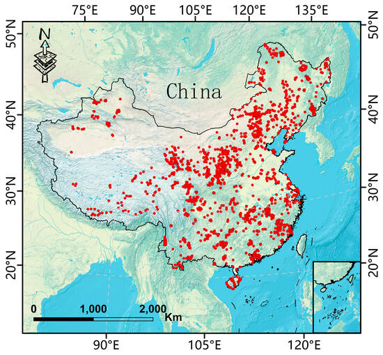
Figure 1.
Geographical distribution of study sites, from 2004 to 2014.
There was a correlation among the 29 selected environmental covariates. It is difficult to explain the impact of the independent effects of the independent variables on the dependent variable, making the model less predictive and also increasing the risk of misclassification. Therefore, we performed multiple covariate analysis to screen the variables to eliminate correlated variables.
The SOC and environmental covariates of the sampling sites were regressed to obtain the matrix of correlation coefficients between the independent variables and the relationship between SOC and the environmental variables [26]. The variance inflation factor (VIF) is a measure of the correlation between independent variables [27]. For each independent variable, its VIF value was calculated. The larger the VIF value, the higher the correlation between SOC and other environmental variables. When determining multicollinearity, usually, when the VIF value of an independent variable is greater than 10, we consider there to be multicollinearity. Based on the VIF value, we determined which independent variables had multicollinearity problems. For independent variables with multicollinearity, one of them needed to be selected for exclusion. We combined the domain knowledge and the actual situation and selected the variable with the highest VIF value to be eliminated and selected the variable that is the least important for the analysis and interpretation to be eliminated. To test the culling effect test, for the rebuilt imputation model, the VIF value was calculated again to ensure that there was no multicollinearity problem after the culling. Based on the VIF value culling results, there were 12 variables left to continue to participate in the next modeling (Table S1).
2.4. Machine Learning Algorithms
2.4.1. Extreme Gradient Boosting (XGBoost)
XGBoost is an efficient and powerful machine learning model that belongs to the gradient boosting framework [28]. XGBoost offers significant improvements in performance and accuracy over traditional gradient boosting models. The core idea is to iteratively train multiple weak learners (usually decision trees) and combine them into one powerful model. In each iteration, XGBoost adjusts the weights of the samples based on the predictions of the previous model, causing the model in the next round to focus more on the samples that were previously incorrectly predicted. This step-by-step optimization process minimizes the model’s loss function, which improves the model’s accuracy [29]. XGBoost has many advantages; it excels in accuracy and can handle various types of data and complex feature relationships. Secondly, XGBoost has high computational efficiency and memory utilization and can handle large-scale datasets and high-dimensional features. The XGBoost package of R 4.2.1 was used for modeling, and the caret package was used to optimally tune the six parameters of learning rate, maximum depth of the tree, minimum loss reduction required to control the splitting of leaf nodes of the tree, percentage of columns randomly sampled to control each tree, total minimum instance weights required in the nodes of the tree, and percentage of random samples randomly sampled to control each tree, and XGBoost was optimally tuned using the xgb. importance to see the importance of the variables.
2.4.2. Light Gradient Boosting Machine (LightGBM)
LightGBM (light gradient boosting machine) is a machine learning algorithm based on the gradient boosting framework, which makes a series of improvements to the classic gradient boosting decision tree (GBDT) algorithm to improve efficiency and scalability [30].The main features of LightGBM are the combination of optimal division points, leaf-wise tree growth strategy, a one-sided gradient sampling technique, and a mutually exclusive feature bundling algorithm. These improvements give LightGBM an advantage in processing large samples and high dimensional data. For processing gradient values, LightGBM uses the one-sided gradient sampling technique (GOSS). It determines the importance of a sample based on its gradient size, retains large gradient sample points, and randomly samples small gradient sample points proportionally. This reduces the number of samples and improves the learning efficiency of the model. In R 4.2.1, we built the model using the lightgbm package. We performed ten-fold cross-validation to optimize the hyperparameter learning rate and the depth of the maximum tree using the bonsai package and the tidymodels package, and we used lgb.importance to see the importance of the variables.
2.4.3. Gradient Boosting Machine (GBM)
The GBM (gradient boosting machine) algorithm is a boosting algorithm. The main idea is to generate multiple weak learners serially, and the goal of each weak learner is to fit the negative gradient of the loss function of the previous cumulative model, so that the loss of the cumulative model after the addition of the weak learner decreases in the direction of the negative gradient [31]. It linearly combines the base learners with different weights so that the learners with excellent performance are reused, and the most commonly used base learner is the tree model. It is robust, interpretable, and efficient regarding noise and outliers. Compared to some deep learning models, GBM models are relatively simple, easier to understand and interpret, and have efficient training and prediction speeds [32].We used the gbm and caret packages in R 4.2.1 for the modeling and optimization of two parameters, tree-tree and single-tree complexity, respectively, using gbm. importance to see the importance of variables.
2.4.4. Random Forest (RF)
Random forest is a commonly used machine learning model for regression problems [33]. It consists of an integrated model comprising multiple decision trees, and the final regression prediction is made by integrating the results of multiple decision trees. Random forests are able to handle not only nonlinear relationships between independent variables and dependent variables with skewed distributions (e.g., SOC) but also a large number of covariates and do not require feature selection. Random forests can also handle missing values and unbalanced data sets. In addition, random forests can also assess the importance of features, helping us to understand which features in the dataset contribute more to the regression results [34]. The model and model parameters were set up in MATLAB 2023a, and the values of the number of nodes in the model (nodesize) and the number of variables in the binary tree (mtry) were adjusted by 10-fold cross-validation to obtain better model performance.
2.4.5. Model Performance
The SOC of the processed sampling points as dependent variables and the optimized environmental variables as independent variables were input into the four machine learning models (XGBoost, GBM, LightGBM, and RF) in Section 2.3 for training modeling, respectively. To ensure the stability of the model predictions, this study performed 10-fold cross-validation on all four models after optimizing the parameters. The index of model selection for predicting organic carbon was then characterized using the weighted characterization of three parameters, root mean square error (RMSE), coefficient of determination (R2), and mapping time cost (t), as follows:
In Equations (1) and (2), y denotes the observed value of SOCD,
denotes the predicted value of SOCD,
denotes the mean of the observed values, and n denotes the number of samples. In Equation (3), t1 represents the mapping time of the model, tmax represents the maximum value of the mapping time of the four models, RMSE1 and RMSEmax represent the root-mean-square error of the model and the maximum value of the RMSE of the four models, respectively, and R2 represents the coefficient of determination of the model.
2.5. SOCD Digital Soil Mapping
The model indices of the four models were calculated, and the model with the index closest to 1 was the optimal model, which was used for the spatial prediction and mapping of SOC on a national scale. The data of environmental variables were inputted into the model, and the estimation of SOC was obtained through the predictive ability of the model. The cross-validation results of the model were taken as mean values to represent the final results of the model. The predicted SOC results were mapped and visualized to generate a spatial distribution map of SOC. Using ArcGIS 10.7, mapping and visualization were performed.
2.6. The Bottom-Up Approach for Vulnerability Analysis
In this study, we employed a bottom-up approach [35] to analyze the sensitivity of SOC to climate change. Utilizing version 2.1 climate models from the World Climate Research Centre and the report published by the IPCC (2021), we examined the projected ranges of precipitation and temperature changes under future climate scenarios. Our focus centered on two shared socioeconomic pathways (SSPs), SSP126 (a low-emission scenario) and SSP585 (a high-emission scenario). Under the SSP126 scenario, global precipitation is expected to vary by approximately 13%, with temperature increases ranging from 0 °C to 1.5 °C [36,37]. In contrast, the SSP585 scenario forecasts precipitation variability as high as 39% and temperature rises of up to 3 °C [36]. To conduct the comprehension of climate change impacts, we constructed an extensive climate change space encompassing a variety of potential scenarios. We established a precipitation change range from −15% to 15% and a temperature increase range from 0 °C to 3 °C, with increments of 1% for precipitation and 0.1 °C for temperature. Utilizing a state-of-the-art machine learning model outlined in Section 2.4, we predicted and estimated SOC levels under each climate scenario, subsequently calculating the differences in SOC across these scenarios. Additionally, we evaluated the sensitivity of SOC under two specific conditions, a standalone temperature increase of 3 °C and a standalone precipitation decrease of 30%, while also quantifying the thresholds for SOC reduction at 10% relative to temperature and precipitation. All data processing and climate scenario modeling were conducted using MATLAB. Through these analyses, we aimed to enhance the understanding of SOC dynamics in response to varying climate change scenarios, thereby providing a scientific basis for future climate adaptation and mitigation strategies.
3. Results
3.1. Statistical Analysis
From the data of SOC statistics of the sampling points, the distribution of the SOC content showed a skewed distribution trend. With the increase of organic carbon density, the number of statistical sampling points showed fluctuating changes, and the distribution of sampling points within different SOC intervals was not uniform. The number of sampling points was relatively high in the organic carbon density interval of 0–5 kg C m−2. In the higher SOCD interval of 10–20 kg C m−2, the number of sampling points was relatively low, which may be limited by the rarity of the samples or limitations in the sampling process (Figure 2).
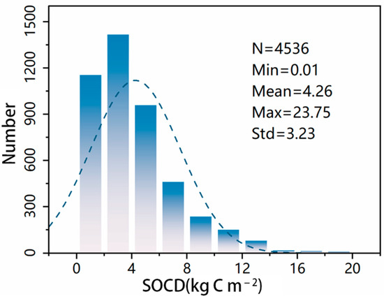
Figure 2.
SOCD statistics for sample sites.
3.2. Model Accuracy and Importance
Regarding model accuracy statistics (Table 2), overall, the RMSE of the model is not much different and is within acceptable range, the decision coefficient of the model is also higher overall, and the time cost of mapping is shorter for XGB and LGB. The modeling with RF has a high accuracy, but its mapping time cost is too high, and the model index is only 0.25, while the accuracy of the XGB model is slightly lower than that of RF. However, its time cost is only 164 s, and the model index reaches 0.55, which is the maximum value of the four models. The variable importance statistics of the four models shows a similar trend, with the most important covariates all being mean air temperature, followed by mean precipitation and net primary productivity of vegetation, and the rest of the variables are almost equal in importance (Figure 3).
Table 2.
Model accuracy statistics.
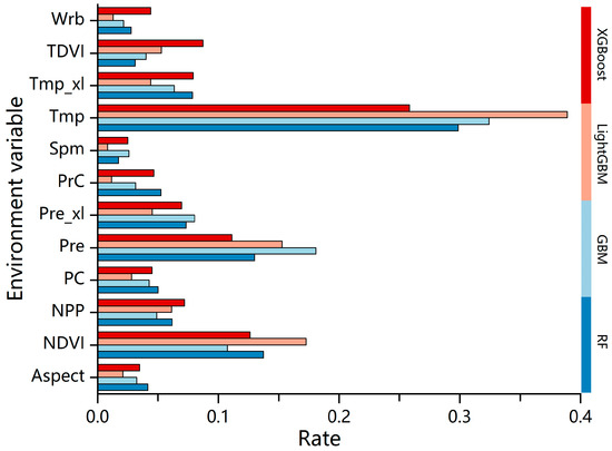
Figure 3.
Variable important statistics of four models. Tvdi_mean, tmp_xl, tmp_mean, Profile Cupre_xl, pre_mean, Plan_Curva, npp_mean, and NDVI_mean represent TDVI mean, tmp slope, tmp mean, contour curvature, pre mean, flat curvature, npp mean, and NDVI mean, respectively.
The fitted scatter plots based on the model predictions and the actual SOC show that the estimated and measured samples from all four modeling methods are distributed along a 1:1 line (Figure 4) and are mostly concentrated in the low value 0–5 (kg C m−2) fraction. The fitted point density plots show similarity, with three centers of higher density. The best fit is RF followed by LightGBM, but the scatter of XGBoost and GBM is a bit more concentrated than RF and LightGBM.
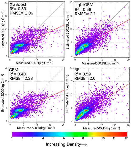
Figure 4.
Scatterplot of measured and estimated SOCD (kg C m−2) for assessing the average model performance of different modeling approaches. The solid gray line represents the 1:1 line. The red line represents the average model performance during the calibration and validation phases. Point density increases gradually from purple to red.
3.3. Spatial Mapping and Uncertainty
Using the model XGBoost (index = 0.55), which has a model index closest to 1, the mapping results presented higher SOC levels locally in Northeast China, Northeast Tibetan Plateau, and Tien Shan Mountains (Figure 5). And the mapping results showed similar spatial distribution patterns to those of the dynamic characteristics of SOC in different soil horizons in China during the 1980s–2010s, as investigated by Li, Wu, Liu, Xiao, Zhao, Chen, Alexandrov and Cao [5], which showed a similar spatial distribution pattern. The national topsoil SOC reserve was calculated to be 4.75 ± 0.53 Pg based on the results of XGBoost, which is consistent with Song et al. [38]. Based on the 2010 national soil dataset (2009–2016, 5696 soil profiles, 23,535 soil samples), the stacked learning framework and five depths were utilized to estimate the organic carbon stock in 1 m soils to be 58.98 Pg, with the subsoil (30–100 cm) accounting for 35.2% of the results being similar.
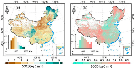
Figure 5.
Extreme Gradient Boost (XGBoost) model predictions. (a) Plot of surface (0–30 cm) SOCD (kg C m−2) at the national spatial scale, with the inset at the bottom left of each panel showing area ratios at different SOC levels. (b) Uncertainty in model estimates. Uncertainty is quantified as the standard deviation of the Extreme Gradient Boost (XGBoost) model simulation for each pixel point. The inset at the bottom left of each panel shows the area ratio at different SOC std levels.
3.4. Climate Sensitivity Analysis
In this study, a bottom-up machine learning approach was used to quantify the sensitivity of SOC to climate change. The results showed that SOC generally showed a trend of decreasing with increasing temperature and increasing with increasing precipitation (Figure 6). Changes in SOC were usually within 10% under different climate scenarios. The largest SOC loss was observed in the scenario with a 3 °C increase in temperature and a 15% decrease in precipitation, while the largest SOC gain was observed in the scenario with a constant temperature and a 15% increase in precipitation. The response to temperature change varied significantly by region, with approximately one-fourth of the nation’s regions experiencing a 10% reduction in SOC for a 1.45 °C temperature increase (Figure 7). The median temperature thresholds for each region are shown in the caption of each figure and range from 1.0 °C to 1.8 °C. For example, Southwest China had the highest median temperature threshold of 1.8 °C, indicating that this region is more tolerant of SOC to elevated temperatures. Central China, on the other hand, has the lowest median of 1.0 °C, indicating that this region is relatively more sensitive to temperature changes. The shape of the density curves shows that the temperature changes in all regions are concentrated in a narrow range, indicating that the temperature threshold changes are relatively concentrated without extreme changes. The curves in all regions show a symmetrical bell shape, indicating that the distribution of temperature threshold changes is close to a normal distribution.
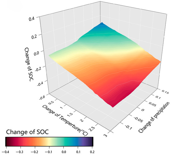
Figure 6.
Changes in simulated SOC content in China under different scenarios.
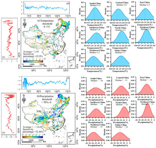
Figure 7.
SOC Sensitivity to temperature and precipitation. (a,b) National climate thresholds under the 10% reduction scenario for SOC; density statistics for temperature and precipitation thresholds across various regions (SC, CC, EC, SW, NC, NE, and NW represent South China, Central China, East China, Southwest China, North China, Northeast China, and Northwest China, respectively). The curves depict the distribution of changes in temperature thresholds, while the blue dashed line indicates the median change in precipitation for each region. (c–f) Changes in longitude and latitude.
A decrease in SOC was more likely to occur at a 3 °C temperature increase in NE China and less likely in NW China. Median values ranged from −18% to −11%, indicating differences in the magnitude of precipitation changes between regions. For example, South China had the lowest median precipitation change of about −18%, indicating that the sensitivity of SOC reductions to precipitation reductions was stronger in this region, whereas Central China and North China had higher median precipitation changes of about −11%, indicating a relatively weaker sensitivity to precipitation changes. The slightly wider distribution in Northwest China may imply that this region has greater uncertainty about precipitation changes. The data from this study provide an important basis for understanding the specific impacts of climate change on SOC in different regions, which can help to develop adaptation strategies and mitigation measures.
4. Discussion
4.1. Model Performance Analysis
We compared the differences between four soil digital mapping methods commonly used in current research. In terms of accuracy, the R2 of the four machine models was within acceptable limits [34,39,40]. In recent years, XGBoost and LightGBM have attracted much attention for their excellent performance in handling large-scale datasets. XGBoost utilizes efficient parallel computing and regularization techniques, which can effectively prevent overfitting and thus improve the generalization ability of the model [41]. At the same time, LightGBM adopts a histogram-based decision tree learning algorithm, which significantly improves the training speed and memory usage efficiency, and it is particularly suitable for big data environments [42]. Comparatively, the traditional GBM, although theoretically flexible and easy to understand, tends to be slower to train in the face of large-scale soil data, and it is suitable for small- and medium-sized datasets [31]. RF excels in many applications due to its robustness regarding outliers and its ability to assess feature significance [43]. However, its training and prediction speed is relatively slow when dealing with large-scale data. In summary, XGBoost and LightGBM usually outperform GBM and RF in large-scale soil mapping, especially when facing complex feature relationships and large data sets. When selecting the best model, the following should be considered: data features, model performance, and terrain characteristics, and systematic comparisons by methods such as cross-validation are recommended to achieve the best soil mapping results.
4.2. SOC Controlling Factors
In all four models, two variables, temperature, and precipitation accounted for a high percentage of importance, with temperature being an important factor influencing the rate of organic carbon decomposition. Higher temperatures accelerate the decomposition process of SOC, resulting in the release of organic carbon to the atmosphere, while lower temperatures slow down the rate of organic carbon decomposition [44,45]. Effects of precipitation on organic carbon storage precipitation is an important regulator of SOC storage [46]. The right amount of precipitation can provide water, promote plant growth and organic matter input, and facilitate the accumulation of SOC. Too much or too little precipitation can lead to loss or decomposition of organic carbon, affecting the accumulation and storage of SOC. SOC is also affected by a combination of many complex factors, including soil microbial activity, enzyme activity, pH, moisture content, temperature, and land use practices [47]. The interaction of these factors makes it difficult to accurately predict organic carbon, and it is still difficult to make machine learning algorithms accurately account for the influencing factors alone.
It was observed that the maximum loss of SOC occurred under scenarios of a 3 °C rise in temperature and a 15% reduction in precipitation. This finding highlights the potential severe threat posed by extreme combinations of increased temperature and decreased moisture to soil carbon stocks in the context of climate change. Such conditions could significantly impair soil ecological functions and agricultural productivity. Notable regional disparities in response to temperature changes are evident, with approximately 25% of regions experiencing a 10% reduction in SOC under a 1.45 °C temperature rise. The southwestern region exhibited a higher resilience to temperature thresholds, while the central region showed relatively greater sensitivity. This finding emphasizes the critical importance of region-specific adaptation strategies; future management practices should take into account local climatic characteristics and soil types to devise more effective response plans. The impact of precipitation changes on SOC also reveals regional variability. The southern regions demonstrate a heightened sensitivity to decreased precipitation, whereas the central and northern regions exhibit a comparatively weaker response. This phenomenon may be closely linked to local soil properties, vegetation cover, and land use practices. In particular, in the southern regions, variations in precipitation may have a more pronounced effect on soil moisture and nutrient dynamics, thereby influencing the stability of SOC.
4.3. Uncertainties and Prospect
We utilized the XGBoost learning algorithm in conjunction with DSM to establish a robust model for predicting surface SOC (0–30 cm) across the country. Despite the overall accuracy, some uncertainties persisted, particularly in the prediction process. To mitigate the impact of human factors, we applied parameter system optimization in the selection and configuration of model parameters. In addition, there are significant topographic differences over the area covered by this study [48], while the spatial distribution of sampling sites and current data resolution remain key constraints. Although topographic factors such as DEM and Slope (2.2 sections) were considered in the analysis method, the local topographic effects and spatial heterogeneity of soil properties may not have been adequately captured due to topographic complexity and insufficient sampling density. Future research will develop a coupled terrain-process model by collecting more data, fusing high-resolution remote sensing data with high-precision DEM data, and combining the strengths of machine learning and process modeling to enhance the reliability of SOC prediction with finer spatial and temporal resolution. This multi-scale fusion approach will effectively reduce terrain-related uncertainties and enhance the robustness of the model under different terrain conditions.
To further improve the accuracy and utility of SOC mapping, future research should prioritize improving data quality, optimizing models, refining feature selection, and the intrinsic mechanisms affecting SOC prediction. In addition, fostering collaboration with policy makers and agricultural producers is essential to translate research results into practical applications and to advance the implementation of sustainable agriculture and environmental protection policies.
5. Conclusions
This study compares the performance of four machine learning models Extreme Gradient Boosting (XGBoost), light gradient boosting machine (LightGBM), gradient boosting machine (GBM), and random forest, in the context of DSM. We utilized the optimal model for predictions and explored climate sensitivity using a bottom-up framework. The results indicate that the XGBoost model outperformed the others, with spatial predictions closely aligning with actual distribution patterns. Variable importance analysis revealed that average temperature and precipitation had the most substantial impact on SOC predictions, followed by the normalized difference vegetation index (NDVI). The influence of other variables was relatively minor. The sensitivity results demonstrated that climate change significantly affects national SOC levels. Even slight increases in temperature can lead to reductions in SOC across the country. We recommend developing appropriate climate adaptation strategies, particularly in regions that are highly sensitive to climate variations. Such strategies can help protect soil carbon stocks and ensure ecological sustainability. They can also enhance the resilience of ecosystems in the face of future climate challenges and uncertainties.
Supplementary Materials
The following supporting information can be downloaded at: https://www.mdpi.com/article/10.3390/su17093965/s1, Table S1. Multiple covariance test.
Author Contributions
Conceptualization, F.L.; data curation, J.G. and Y.M.; formal analysis, B.M.; funding acquisition, L.W.; investigation, F.L.; methodology, F.L.; project administration, L.W.; resources, J.G. and Y.M.; software, J.C. and B.M.; supervision, L.W.; validation, B.M. and F.H.; visualization, J.C. and J.Z.; writing–original draft, J.C.; writing–review and editing, J.Z. All authors have read and agreed to the published version of the manuscript.
Funding
Investigation: Monitoring and Evaluation of Desert Salinisation and Ecological Restoration in the Northern Tarim River Basin (DD20220887), Open Project of the Key Laboratory of Coupled Processes and Effects of Natural Resource Elements, Ministry of Natural Resources (2022KFKTC010).
Institutional Review Board Statement
Not applicable.
Informed Consent Statement
Not applicable.
Data Availability Statement
The original contributions presented in this study are included in the article/Supplementary Material. Further inquiries can be directed to the corresponding author.
Acknowledgments
We thank all the field investigators, the subject editor, and anonymous reviewers for their insightful comments and suggestions for this manuscript.
Conflicts of Interest
The authors declare that they have no competing financial interests or personal relationships that may have influenced the work reported in this study.
References
- Hou, S.; Bai, Y.; Wang, C.; Zu, C.; Zhang, R.; Wang, X. Progress in the study of soil organic carbon and its active components. Jiangsu Agric. Sci. 2023, 51, 24–33. [Google Scholar] [CrossRef]
- Zhang, G.; Shi, Z.; Zhu, A.; Wang, Q.; Wu, K.; Shi, Z.; Zhao, Y.; Zhao, Y.; Pan, X.; Liu, F.; et al. Progress and Perspective of Studies on Soils in Space and Time. Acta Pedol. Sin. 2020, 57, 1060–1070. [Google Scholar]
- Wang, S.; Xu, L.; Adhikari, K.; He, N. Soil carbon sequestration potential of cultivated lands and its controlling factors in China. Sci. Total Environ. 2023, 905, 167292. [Google Scholar] [CrossRef] [PubMed]
- Zhang, Z.; Ding, J.; Zhu, C.; Chen, X.; Wang, J.; Han, L.; Ma, X.; Xu, D. Bivariate empirical mode decomposition of the spatial variation in the soil organic matter content: A case study from NW China. Catena 2021, 206, 105572. [Google Scholar] [CrossRef]
- Li, H.; Wu, Y.; Liu, S.; Xiao, J.; Zhao, W.; Chen, J.; Alexandrov, G.; Cao, Y. Decipher soil organic carbon dynamics and driving forces across China using machine learning. Glob. Change Biol. 2022, 28, 3394–3410. [Google Scholar] [CrossRef]
- Zhang, L.; Heuvelink, G.B.M.; Mulder, V.L.; Chen, S.; Deng, X.; Yang, L. Using process-oriented model output to enhance machine learning-based soil organic carbon prediction in space and time. Sci. Total Environ. 2024, 922, 170778. [Google Scholar] [CrossRef]
- Su, H. Dimensionality reduction for hyperspectral remote sensing: Advances, challenges, and prospects. Natl. Remote Sens. Bull. 2022, 26, 1504–1529. [Google Scholar] [CrossRef]
- McBratney, A.B.; Mendonça Santos, M.L.; Minasny, B. On digital soil mapping. Geoderma 2003, 117, 3–52. [Google Scholar] [CrossRef]
- Zhu, A.; Yang, L.; Fan, N.; Tsang, C.-y.; Zhang, G. The review and outlook of digital soil mapping. Prog. Geogr. 2018, 37, 66–78. [Google Scholar]
- Popa, A.; Popa, I.; Badea, O.; Bosela, M. Non-linear response of Norway spruce to climate variation along elevational and age gradients in the Carpathians. Environ. Res. 2024, 252, 119073. [Google Scholar] [CrossRef]
- Zhang, Z.; Ding, J.; Zhu, C.; Wang, J.; Ge, X.; Li, X.; Han, L.; Chen, X.; Wang, J. Historical and future variation of soil organic carbon in China. Geoderma 2023, 436, 116557. [Google Scholar] [CrossRef]
- Sun, Z.; Xue, L.; Xu, Y.; Wang, Z. Overview of deep learning. Appl. Res. Comput. 2012, 29, 2806–2810. [Google Scholar]
- Zhang, Z.; Ding, J.; Zhu, C.; Shi, H.; Chen, X.; Han, L.; Wang, J. Changes in soil organic carbon stocks from 1980–1990 and 2010–2020 in the northwest arid zone of China. Land Degrad. Dev. 2022, 33, 2713–2727. [Google Scholar] [CrossRef]
- Shuai, M.; Tong, T.; Chunyang, Y.; Sweetie, W.; Mei, Z.; Mengmeng, T.; Tianpei, C.; Youhua, M.; Qiang, W. Advances in digital soil mapping based on machine learning. J. Agric. Resour. Environ. 2023, 41, 774. [Google Scholar] [CrossRef]
- Hengl, T.; de Jesus, J.M.; MacMillan, R.A.; Batjes, N.H.; Heuvelink, G.B.M.; Ribeiro, E.; Samuel-Rosa, A.; Kempen, B.; Leenaars, J.G.B.; Walsh, M.G.; et al. SoilGrids1km—Global Soil Information Based on Automated Mapping. PLoS ONE 2014, 9, e105992. [Google Scholar] [CrossRef]
- Zhang, G.-l.; Liu, F.; Song, X.-d. Recent progress and future prospect of digital soil mapping: A review. J. Integr. Agric. 2017, 16, 2871–2885. [Google Scholar] [CrossRef]
- Geremew, B.; Tadesse, T.; Bedadi, B.; Gollany, H.T.; Tesfaye, K.; Aschalew, A.; Tilaye, A.; Abera, W. Evaluation of RothC model for predicting soil organic carbon stock in north-west Ethiopia. Environ. Chall. 2024, 15, 100909. [Google Scholar] [CrossRef]
- Zhou, Y.; Chen, S.; Zhu, A.X.; Hu, B.; Shi, Z.; Li, Y. Revealing the scale- and location-specific controlling factors of soil organic carbon in Tibet. Geoderma 2021, 382, 114713. [Google Scholar] [CrossRef]
- Padarian, J.; Minasny, B.; McBratney, A.B. Machine learning and soil sciences: A review aided by machine learning tools. Soil 2020, 6, 35–52. [Google Scholar] [CrossRef]
- Pathak, R.; Dasari, H.P.; Ashok, K.; Hoteit, I. Effects of multi-observations uncertainty and models similarity on climate change projections. npj Clim. Atmos. Sci. 2023, 6, 144. [Google Scholar] [CrossRef]
- Thuiller, W.; Guéguen, M.; Renaud, J.; Karger, D.N.; Zimmermann, N.E. Uncertainty in ensembles of global biodiversity scenarios. Nat. Commun. 2019, 10, 1446. [Google Scholar] [CrossRef] [PubMed]
- Wang, Q.; Shan, Y.; Shi, W.; Zhao, F.; Li, Q.; Sun, P.; Wu, Y. Assessing spatiotemporal variations of soil organic carbon and its vulnerability to climate change: A bottom-up machine learning approach. Clim. Smart Agric. 2024, 1, 100025. [Google Scholar] [CrossRef]
- Singh, R.; Kumar, R. Vulnerability of water availability in India due to climate change: A bottom-up probabilistic Budyko analysis. Geophys. Res. Lett. 2015, 42, 9799–9807. [Google Scholar] [CrossRef]
- Zhao, F.; Wu, Y.; Qiu, L.; Sun, Y.; Sun, L.; Li, Q.; Niu, J.; Wang, G. Parameter Uncertainty Analysis of the SWAT Model in a Mountain-Loess Transitional Watershed on the Chinese Loess Plateau. Water 2018, 10, 690. [Google Scholar] [CrossRef]
- Xu, L.; Nianpeng, H.; Yu, G. A dataset of carbon density in Chinese terrestrial ecosystems (2010s). CSData 2019, 4, 90–96. [Google Scholar] [CrossRef]
- Zhu, C.; Li, Y.; Ding, J.; Rao, J.; Xiang, Y.; Ge, X.; Wang, J.; Wang, J.; Chen, X.; Zhang, Z. Spatiotemporal analysis of AGB and BGB in China: Responses to climate change under SSP scenarios. Geosci. Front. 2025, 16, 102038. [Google Scholar] [CrossRef]
- Chan, Y.; Liang, T.; Zhang, Y.; Wang, Y.; Yuan, D.; Zhu, J.; Li, D. Spatial Prediction of Soil Thicknesses in Sichuan Province Based on Feature-Ensemble Learning. Soils 2023, 55, 894–902. [Google Scholar] [CrossRef]
- Wang, S.C.; Huo, Y.; Mu, X.; Jiang, P.; Zhu, L.; Xun, S.; He, B.; Wu, W. Estimation of surface NO2 concentration in China based on extreme gradient boosted tree and deep learning methods. Acta Sci. Circumstantiae 2023, 43, 298–308. [Google Scholar] [CrossRef]
- Chen, T.; Jiao, J.; Zhang, Z.; Lin, H.; Zhao, C.; Wang, H. Soil quality evaluation of the alluvial fan in the Lhasa River Basin, Qinghai-Tibet Plateau. Catena 2022, 209, 105829. [Google Scholar] [CrossRef]
- Ju, Y. Carbon Emission Forecasting in China Based on Spatio-Temporal LightGBM Models. Master’s Thesis, Nanjing Post and Communications University, Nanjing, China, 2023. [Google Scholar]
- Friedman, J.H.J.A.o.S. Greedy function approximation: A gradient boosting machine. Ann. Stat. 2001, 29, 1189–1232. [Google Scholar] [CrossRef]
- Natekin, A.; Knoll, A. Gradient boosting machines, a tutorial. Front. Neurorobotics 2013, 7, 21. [Google Scholar] [CrossRef] [PubMed]
- Speiser, J.L.; Miller, M.E.; Tooze, J.; Ip, E. A comparison of random forest variable selection methods for classification prediction modeling. Expert Syst. Appl. 2019, 134, 93–101. [Google Scholar] [CrossRef] [PubMed]
- Zhang, Z.; Ding, J.; Zhu, C.; Wang, J.; Li, X.; Ge, X.; Han, L.; Chen, X.; Wang, J. Exploring the inter-decadal variability of soil organic carbon in China. Catena 2023, 230, 107242. [Google Scholar] [CrossRef]
- Li, C.; Frolking, S.; Frolking, T.A. A model of nitrous oxide evolution from soil driven by rainfall events: 1. Model structure and sensitivity. J. Geophys. Res. Atmos. 1992, 97, 9759–9776. [Google Scholar] [CrossRef]
- Piao, S.; Ciais, P.; Huang, Y.; Shen, Z.; Peng, S.; Li, J.; Zhou, L.; Liu, H.; Ma, Y.; Ding, Y.; et al. The impacts of climate change on water resources and agriculture in China. Nature 2010, 467, 43–51. [Google Scholar] [CrossRef] [PubMed]
- Yaduvanshi, A.; Nkemelang, T.; Bendapudi, R.; New, M. Temperature and rainfall extremes change under current and future global warming levels across Indian climate zones. Weather Clim. Extrem. 2021, 31, 100291. [Google Scholar] [CrossRef]
- Song, X.-D.; Wu, H.-Y.; Ju, B.; Liu, F.; Yang, F.; Li, D.-C.; Zhao, Y.-G.; Yang, J.-L.; Zhang, G.-L. Pedoclimatic zone-based three-dimensional soil organic carbon mapping in China. Geoderma 2020, 363, 114145. [Google Scholar] [CrossRef]
- Zhang, X.; Xue, J.; Chen, S.; Wang, N.; Shi, Z.; Huang, Y.; Zhuo, Z. Digital Mapping of Soil Organic Carbon with Machine Learning in Dryland of Northeast and North Plain China. Remote Sens. 2022, 14, 2504. [Google Scholar] [CrossRef]
- Li, Y.; Ru, s.; Zhao, T.; Yuan, J.; Liu, Y.; Lu, G.; Zhang, P. Advances in digital soil mapping methods. Chin. Agric. Sci. Bull. 2024, 40, 146–153. [Google Scholar] [CrossRef]
- Chen, T.; Guestrin, C. XGBoost: A Scalable Tree Boosting System. In Proceedings of the 22nd ACM SIGKDD International Conference on Knowledge Discovery and Data Mining, San Francisco, CA, USA, 13–17 August 2016; pp. 785–794. [Google Scholar]
- Ke, G.; Meng, Q.; Finley, T.; Wang, T.; Chen, W.; Ma, W.; Ye, Q.; Liu, T.-Y. LightGBM: A Highly Efficient Gradient Boosting Decision Tree. In Proceedings of the Neural Information Processing Systems, Long Beach, CA, USA, 4–9 December 2017. [Google Scholar]
- Breiman, L. Random Forests. Mach. Learn. 2001, 45, 5–32. [Google Scholar] [CrossRef]
- Wang, M.; Guo, X.; Zhang, S.; Xiao, L.; Mishra, U.; Yang, Y.; Zhu, B.; Wang, G.; Mao, X.; Qian, T.; et al. Global soil profiles indicate depth-dependent soil carbon losses under a warmer climate. Nat. Commun. 2022, 13, 5514. [Google Scholar] [CrossRef] [PubMed]
- Ai, J.; Zhang, Z.; Yang, C.; Cao, J.; Zhou, Z.; Ge, X.; Chen, X.; Wang, J. Unveiling the Dynamic Patterns and Driving Forces of Soil Organic Carbon in Chinese Croplands From 1980 to 2020. Land Degrad. Dev. 2025, 1085–3278. [Google Scholar] [CrossRef]
- Chen, X.; Liu, J.; Deng, Q.; Chu, K.W.; Zhou, G.; Zhang, D. Effects of precipitation intensity on soil organic carbon fractions and their distribution under subtropical forests of South China. Chin. J. Appl. Ecol. 2010, 21, 1210–1216. [Google Scholar] [CrossRef]
- Qian, Z. A Review of Research on Soil Organic Carbon Stocks and Their Drivers. J. Guangdong Seric. 2022, 56, 35–38. [Google Scholar]
- Cheng, W.; Zhou, C.; Li, B.; Shen, Y.; Zhang, B. Structure and contents of layered classification system of digital geomorphology for China. J. Geogr. Sci. 2011, 21, 771–790. [Google Scholar] [CrossRef]
Disclaimer/Publisher’s Note: The statements, opinions and data contained in all publications are solely those of the individual author(s) and contributor(s) and not of MDPI and/or the editor(s). MDPI and/or the editor(s) disclaim responsibility for any injury to people or property resulting from any ideas, methods, instructions or products referred to in the content. |
© 2025 by the authors. Licensee MDPI, Basel, Switzerland. This article is an open access article distributed under the terms and conditions of the Creative Commons Attribution (CC BY) license (https://creativecommons.org/licenses/by/4.0/).