The Green Paradox of New Energy Vehicles: A System Dynamics Analysis

Abstract

New energy vehicles produce zero tailpipe emissions and are an effective method for addressing traffic pollution. This study establishes a system dynamics management model to explore the mid- and long-term effects of the new energy vehicle promotion policy on urban traffic and environment. Additionally, we propose a nonlinear function optimization algorithm integrating system dynamics with an optimized even difference grey model to improve the model’s accuracy and validity. The dynamic simulation results show that (1) promoting new energy vehicles reduces tailpipe emissions and alleviates traffic pollution but may lead to a “green paradox” effect in the long term. Positive traffic control measures, such as driving restrictions, accelerate the “substitution effect” of new energy vehicles, and congestion and fuel consumption show a “rebound effect” in later stages. (2) A congestion charging policy reduces vehicle travel attractiveness and alleviates congestion. A sensitivity analysis indicates that a reasonable charging range is 20–40 yuan/(day × vehicle). (3) Introducing congestion charging and improving public transport supply level can effectively weaken the “paradox” effect. This combination not only mitigates congestion and pollution but also reduces economic losses and improves residents’ health. The strategy has a “lag effect” in the early stage but shows effectiveness in the middle (congestion alleviation) and later (pollution control) stages.

1. Introduction

Problems related to urban traffic and pollution have become more serious in recent years. Severe congestion increases fuel consumption and exhaust emissions, aggravating “smog” pollution and harming residents’ health [1]. The main pollutants in vehicle exhaust include CO, HC, NO_X, and PM, with NO_X and PM raising the incidence of cardiovascular and respiratory diseases and increasing urban mortality [2,3]. Worldwide exposure to PM_2.5 causes over 4 million premature deaths annually [4]. According to official statistics [5], automobiles are the main contributors to total emissions of pollutants, accounting for over 90% of CO, HC, NO_X and PM emissions. The statistical data indicate that traffic pollution from vehicle exhaust emissions cannot be ignored.

In order to alleviate traffic pollution, many countries have adopted technological means to reduce vehicle emissions. Replacing conventional vehicles with new energy vehicles (NEVs) is an effective strategy for reducing PM_2.5 [6], CO₂ [7] and other emissions such as NO_X [8,9]. NEVs are characterized by their utilization of non-traditional fuel sources or advanced onboard power systems. From a technological perspective, NEVs can be categorized into battery electric vehicles (BEVs), plug-in hybrid electric vehicles (PHEVs), and fuel cell electric vehicles (FCEVs) based on their powertrain systems [10]. In 2024, China’s NEV sales consisted of 60.00% BEVs, 39.95% PHEVs, and 0.05% FCEVs [11]. These vehicle types exhibit different impacts on the “green paradox”; while BEVs produce zero operational emissions, they generate emissions during battery production and disposal from a lifecycle perspective [12]. Additionally, their large-scale charging demands increase electricity loads and may elevate coal power usage [13]. PHEVs produce emissions when switching to fuel mode after battery depletion, and FCEVs face limitations from the underdeveloped hydrogen refueling network [10]. These variations imply that different NEV technologies have varying impacts on social and environmental benefits, requiring consideration in policy design. To increase NEV market share, many governments have implemented incentive policies. The Zero Emission Vehicle Program in California mandates reductions in fossil fuel consumption [14]. Various fiscal incentives, including import tax exemptions (Thailand), consumption tax reductions (Malaysia), and congestion charge exemptions (UK), have promoted NEV development [15]. In China, the government has introduced policies including purchase tax exemptions, subsidies for vehicle purchases, and free charging services. Notably, in June 2023, the Ministry of Industry and Information Technology [16] announced the extension of NEV purchase tax policies, offering full exemptions (up to ¥30,000) for vehicles purchased between 2024 and 2025 and a 50% reduction (up to ¥15,000) for vehicles purchased from 2026 to 2027. Meanwhile, local governments have also proposed incentive policies (e.g., vehicle replacement subsidies, purchase/driving restrictions removal, and parking discounts) as a complement to national-level policies [17]. These incentive measures have stimulated consumer demand, increased NEV sales, and accelerated the NEV industry growth.

The potential impact of NEVs on urban air pollution has garnered significant academic attention in recent years. The current research focuses on policy incentives and life-cycle analysis. Firstly, the main incentive policies include economic (e.g., subsidies) and non-economic incentives (e.g., purchase and driving restrictions removal). Studies have shown that NEV subsidies reduce vehicle emissions [18,19], decrease fuel consumption [20], and improve air quality [6]. These subsidies facilitate the replacement of conventional vehicles with NEVs, yielding environmental and economic benefits [21]. Li and Zhang [6] found that subsidies significantly improved air quality. Driving and purchase restrictions influence the relationship between NEVs and air quality. Wu et al. [22] argued that NEV subsidies and driving restrictions reduce pollution by stimulating NEV purchase and alleviating congestion. However, in the long run, driving restrictions may trigger new car purchases, leading to a rebound in traffic pollution and paradoxical effects [23]. Yang et al. [17] found that the combination of purchase-quota-limit policy and NEV promotion would have obvious emission reduction and healthy economic benefits. Secondly, life-cycle analysis quantifies both tangible and intangible costs alongside environmental benefits throughout the NEVs’ lifecycle. For example, Wu et al. [24] showed that pollution from coal-fired power plants manufacturing batteries could offset NEVs’ operational benefits. Considering power generation cleanliness, NEVs currently do not reduce emissions [25,26]. Compared to fuel vehicles, NEVs reduce energy consumption and emissions during operation but require substantial energy during production. Optimizing power generation and enhancing battery recycling can reduce pollution control costs and improve environmental benefits [12,27]. These studies provide a theoretical foundation for improving urban transport emission and pollution control policies.

While NEVs demonstrate zero operational emissions, concerns remain about the impact of the surge in NEV numbers on urban traffic efficiency and road capacity. To promote NEV adoption, many local governments in China have implemented policies exempting NEVs from driving restrictions and license plate quotas. For example, Beijing uses a lottery for conventional fuel vehicles while relaxing restrictions for NEVs. In July 2024, Beijing allocated 20,000 NEV licenses to car-free families. Major cities like Beijing, Tianjin and Chengdu have implemented driving restrictions for fuel vehicles while exempting NEVs. These policies have facilitated the transition from internal combustion engine vehicles to NEVs, influencing urban transportation development. For example, Ma et al. [28] developed a multivariate co-integration model to assess the short- and long-term effects of NEV sales and driving policies. The results indicated a positive relationship between NEV market share and subsidies, tax exemption, fuel vehicle purchase restrictions, and the removal of traffic restrictions for NEVs. China’s driving restrictions on fuel vehicles influence consumer choices through supply–demand regulation, thereby promoting NEV sales. The subsidy policy has improved NEV competitiveness, but it is not a long-term solution. Alternative incentives are needed as subsidies are gradually phased out [29]. The removal of subsidies could lead to a 42% decline in NEV market share by 2030, negatively impacting sales [30]. Alternative incentives can weaken the negative impact of subsidy removal and promote long-term NEV growth [31].

However, the growing market penetration and utilization frequency of NEVs may induce extra traffic congestion [32]. Ju et al. [33] argued that exempting NEVs from driving restrictions would increase vehicle travel numbers, exacerbating congestion. To this end, Wang et al. [32] and Jia and Yan [34] proposed two interventions: separating gasoline and electric vehicle commuters and implementing a congestion charging policy (CCP). Several countries have implemented CCP. For example, Singapore launched its electronic road pricing (ERP) system in 1998, charging vehicles based on the distance traveled in congested areas [35]. This policy has shifted public commuting habits, reduced traffic volume, and maintained acceptable road speeds. The ERP’s success is due to an efficient public transport network, which has increased ridership and public satisfaction. In contrast, London saw an initial traffic reduction after implementing CCP, but congestion levels eventually rebounded. Chen et al. [36] analyzed the causes of the rebound effect and found that charging fees would increase travelers’ perception of psychological loss. Travelers who choose to pay will regard charging as sunk cost, affecting car trips, aggravating congestion, and producing side effects. Public publicity and public transport priority policies can regulate vehicle usage and generate economic benefits. Moving beyond policy instruments, emerging technological solutions, such as vehicle platooning, offer novel approaches to optimize traffic flow and mitigate congestion. Specifically, recent studies [37,38,39] have demonstrated that coordinating clustered vehicles through intelligent control systems can enhance road capacity and stability. Viadero-Monasterio et al. [37] developed a fault-tolerant control framework for heterogeneous EV platoons that robustly handles measurement noise and disturbances, significantly enhancing platoon cohesion and stability under diverse operating conditions. In another study, Viadero-Monasterio et al. [38] proposed a static output–feedback control strategy that maintains stable coordination despite vehicle mass uncertainties, demonstrating through simulations that it effectively minimizes spacing errors while simplifying communication architecture. Furthermore, Xiao et al. [39] investigated stability control strategies for high-speed steering platoons, analyzing how vehicle dynamics and steering parameters affect system stability, which provides crucial insights for implementing platoons in real-world traffic scenarios. These approaches collectively enhance road safety and traffic efficiency while offering viable strategies for future intelligent transportation systems. The above research proposes policy and technological solutions to alleviate road congestion and optimize traffic flow, offering significant reference value and practical implications. These findings provide new ideas for subsequent research.

To summarize, the existing studies primarily focus on the impact of NEV subsidies and development on urban air quality and pollution control, with limited attention to traffic congestion. Some research explores traveler behavior from behavioral economic perspectives but rarely incorporate NEVs and lack a dual focus on congestion mitigation and pollution control when assessing medium- and long-term policy effects. Meanwhile, several critical questions also warrant further study: (1) While NEVs positively impact pollution mitigation, might they induce traffic-related side effects or a “green paradox” effect in the long term? (2) If such effects exist, how can they be mitigated and policies optimized? The problems are studied in detail in this study. The existing studies mainly adopt econometric methods relying on historical data, often neglecting the dynamic and interdependent nature of complex systems. Policy impacts on society, transportation, and the environment are nonlinear, dynamic, and influenced by feedback mechanisms. Consequently, it is crucial not only to consider historical data but also to gain insights into future trends and explore the medium- and long-term effects of policies. System dynamics (SD) can address the above problems by integrating qualitative analysis (causal analysis) and quantitative analysis (policy simulation) to enable medium- and long-term dynamic simulations. Grey system theory [40] further enhances SD models by extracting valuable information from available data, improving model accuracy and effectiveness.

In consideration of the above, this study intends to carry out the following work: First, an urban congestion mitigation and pollution control (CMPC) management model considering traffic policy is established by using the SD method. Then, a nonlinear function optimization algorithm that integrates SD with the optimized even difference grey model (SD-OEDGM) is proposed to overcome the deficiency of partial validation and improve the accuracy and effectiveness of the model. Finally, dynamic simulation is conducted by adjusting parameters to explore the mid- and long-term effects of the NEV promotion policy. Scenario optimization and sensitivity analysis are performed to propose policy recommendations.

The main contributions of this study are as follows: Firstly, the SD-OEDGM method is used to explore the effects of the NEV promotion policy from multiple perspectives. This study not only considers the degree of congestion mitigation (social benefit) and pollution control (environmental benefit) but also discusses policy effects on reducing GDP loss (economic benefit) and improving public health (health benefit). Secondly, through mid- and long-term dynamic simulation, this study reveals the substitution, green paradox, and rebound effects of the NEV promotion policy and analyzes the lag effect in the early stage and the effectiveness in the later stage of combination strategy. These findings can provide a theoretical reference for the governance of urban CMPC.

2. Materials and Methods

2.1. System Dynamics

System dynamics (SD), established by Professor Jay W. Forrester in 1956 [41], serves as a methodology for addressing nonlinear, high-order complex system problems through feedback control theory and computer simulation technology. It has been widely applied in many fields, such as airport operation [41], water management issues [42], carbon emission reduction [43], and information security [44]. In addition, considering some deficiencies in SD modeling—such as the need to improve model accuracy and data and modeling process rigor—many scholars have combined SD with other methods, such as game theory [45], gray incidence analysis [34], and econometrics [18]. This approach reduces defects and enhances model precision and accuracy.

2.2. Model Development

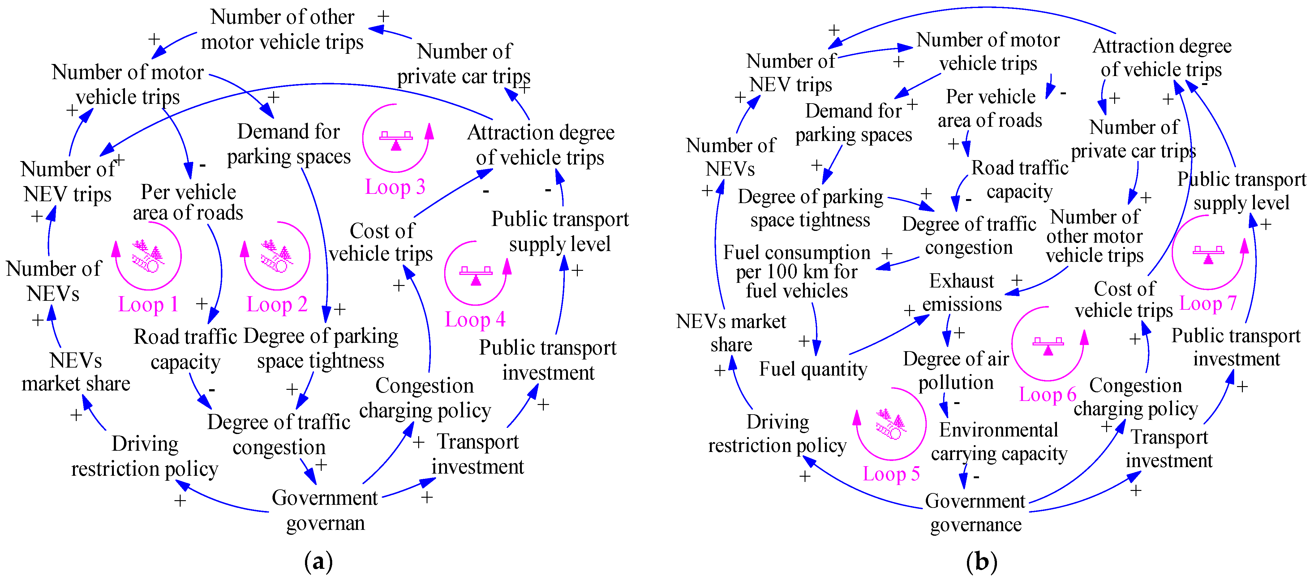
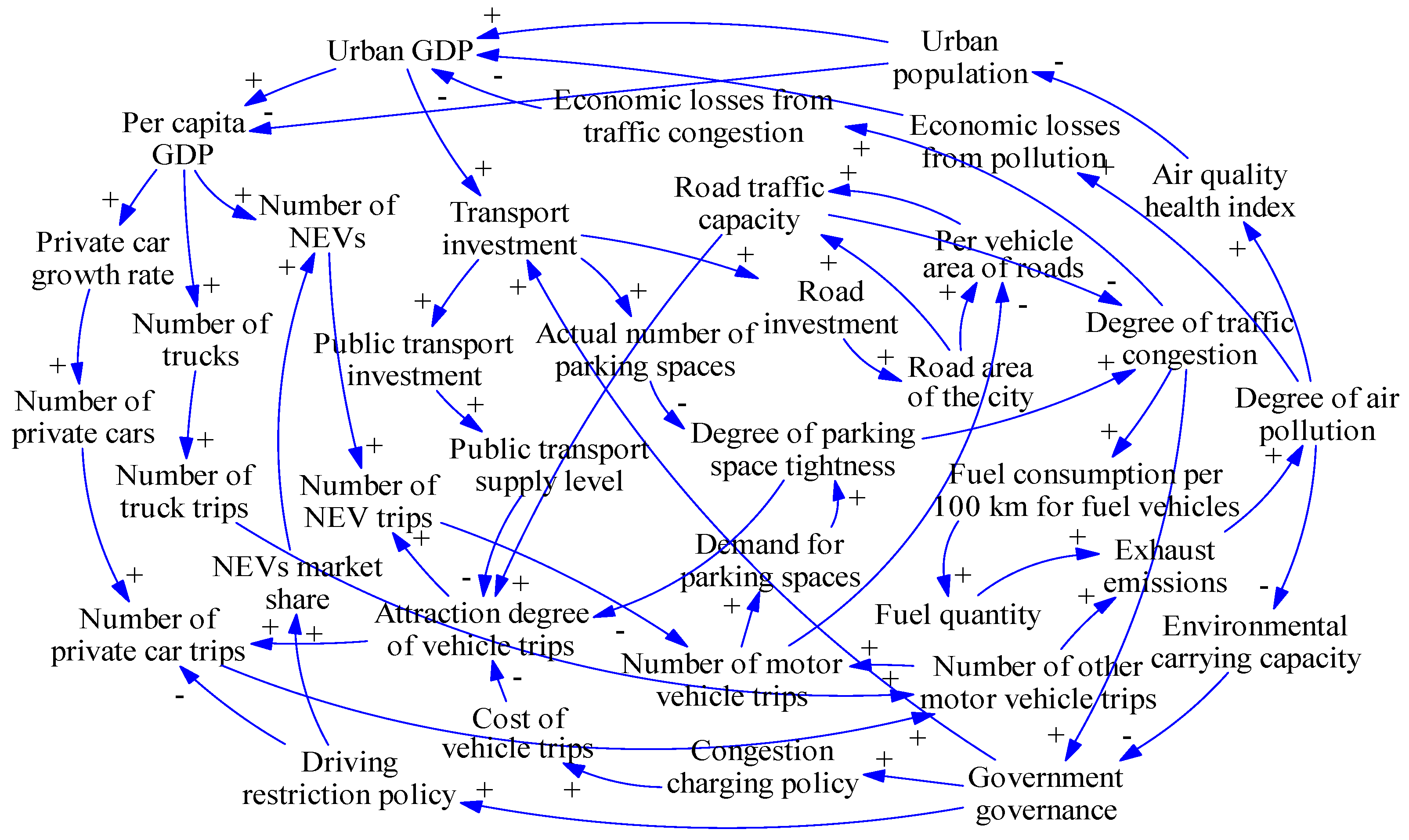
2.2.1. Causal Loop Analysis

A causal loop diagram is used to qualitatively describe the causal relationships and interactions between variables. The urban CMPC management model is a complex dynamic system involving multiple elements. Based on the system modeling objectives, the model is divided into five subsystems: society, economy, transportation, environment, and health. According to the actual situation and existing research, seven main feedback loops are constructed using VENSIM 5.8 software through the analysis of the causal relationship between subsystems and variables, as shown in Figure 1. There are three positive feedback loops (self-reinforcing) and four negative feedback loops (balancing). The causal loop diagram of the urban CMPC management model is shown in Figure 2.

The main feedback loops are as follows:

Loop1: Degree of traffic congestion (DTC)$\stackrel{+}{\to }$Government governance$\stackrel{+}{\to }$Driving restriction policy$\stackrel{+}{\to }$NEVs market share$\stackrel{+}{\to }$Number of NEVs$\stackrel{+}{\to }$Number of NEV trips$\stackrel{+}{\to }$Number of motor vehicle trips$\stackrel{-}{\to }$Per vehicle area of roads (PVAR)$\stackrel{+}{\to }$Road traffic capacity (RTC)$\stackrel{-}{\to }$DTC.

Loop2: DTC$\stackrel{+}{\to }$Government governance$\stackrel{+}{\to }$Driving restriction policy$\stackrel{+}{\to }$NEVs market share$\stackrel{+}{\to }$Number of NEVs$\stackrel{+}{\to }$ Number of NEV trips$\stackrel{+}{\to }$Number of motor vehicle trips$\stackrel{+}{\to }$Demand for parking spaces$\stackrel{+}{\to }$Degree of parking space tightness$\stackrel{+}{\to }$DTC.

Loop3: DTC$\stackrel{+}{\to }$Government governance$\stackrel{+}{\to }$CCP$\stackrel{+}{\to }$Cost of vehicle trips$\stackrel{-}{\to }$Attraction degree of vehicle trips$\stackrel{+}{\to }$Number of private car trips$\stackrel{+}{\to }$Number of other motor vehicle trips$\stackrel{+}{\to }$Number of motor vehicle trips$\stackrel{-}{\to }$PVAR$\stackrel{+}{\to }$RTC$\stackrel{-}{\to }$DTC.

Loop4: DTC$\stackrel{+}{\to }$Government governance$\stackrel{+}{\to }$Transport investment$\stackrel{+}{\to }$Public transport investment$\stackrel{+}{\to }$Public transports supply level$\stackrel{-}{\to }$Attraction degree of vehicle trips$\stackrel{+}{\to }$Number of NEV trips$\stackrel{+}{\to }$Number of motor vehicle trips$\stackrel{-}{\to }$PVAR$\stackrel{+}{\to }$ RTC$\stackrel{-}{\to }$DTC.

Loop5: Degree of air pollution (DAP)$\stackrel{-}{\to }$Environmental carrying capacity (ECC)$\stackrel{-}{\to }$ Government governance$\stackrel{+}{\to }$ Driving restriction policy$\stackrel{+}{\to }$NEVs market share$\stackrel{+}{\to }$Number of NEVs$\stackrel{+}{\to }$Number of NEV trips$\stackrel{+}{\to }$Number of motor vehicle trips$\stackrel{-}{\to }$PVAR$\stackrel{+}{\to }$RTC$\stackrel{-}{\to }$DTC$\stackrel{+}{\to }$Fuel consumption per 100 km for fuel vehicles$\stackrel{+}{\to }$Fuel quantity$\stackrel{+}{\to }$Exhaust emissions$\stackrel{+}{\to }$DAP.

Loop6: DAP$\stackrel{-}{\to }$ECC$\stackrel{-}{\to }$Government governance$\stackrel{+}{\to }$CCP$\stackrel{+}{\to }$Cost of vehicle trips$\stackrel{-}{\to }$Attraction degree of vehicle trips$\stackrel{+}{\to }$Number of private car trips$\stackrel{+}{\to }$Number of other motor vehicle trips$\stackrel{+}{\to }$Exhaust emissions$\stackrel{+}{\to }$DAP.

Loop7: DAP$\stackrel{-}{\to }$ECC$\stackrel{-}{\to }$Government governance$\stackrel{+}{\to }$Transport investment$\stackrel{+}{\to }$Public transport investment$\stackrel{+}{\to }$Public transport supply level$\stackrel{-}{\to }$Attraction degree of vehicle trips$\stackrel{+}{\to }$Number of NEV trips$\stackrel{+}{\to }$Number of motor vehicle trips$\stackrel{+}{\to }$Demand for parking spaces$\stackrel{+}{\to }$Degree of parking space tightness$\stackrel{+}{\to }$DTC$\stackrel{+}{\to }$Fuel consumption per 100 km for fuel vehicles$\stackrel{+}{\to }$Fuel quantity$\stackrel{+}{\to }$Exhaust emissions$\stackrel{+}{\to }$DAP.

Loop 1 and Loop 2 are positive feedback loops. In Loop 1, the continuous increase in DTC prompts the government to adopt a driving restriction policy to reduce the number of motor vehicle trips. However, based on the reality and existing research [29], we find that the restriction applies only to conventional fuel vehicles while exempting NEVs; stricter enforcement will influence consumer behavior, leading some residents to purchase NEVs [46]. This will increase NEVs’ market share and the number of motor vehicle trips, leading to a reduction in PVAR and ultimately exacerbating DTC [47]. A similar analysis can be applied to Loop 2. The increase in the number of vehicle trips requires more parking spaces, and the shortage of parking spaces will further aggravate DTC. This causal relationship has been verified in the existing research [48]. Furthermore, severe congestion will lead to frequent deceleration and braking of vehicles, which increases fuel consumption per 100 km for fuel vehicles and exhaust emissions [49], thereby exacerbating DAP (see Loop 5).

Loop 3 and Loop 6 are negative feedback loops. To overcome the limitations of the above policy, CCP is introduced first. Based on empirical evidence [34], by increasing travel costs, CCP reduces the attraction degree of vehicle trips and decreases the number of motor vehicle trips, thereby alleviating DTC. This causal mechanism can be observed in urban case studies [28]. The implementation of this economic measure can not only alleviate congestion and reduce pollutant emissions but also effectively curb haze pollution (see Loop 6). Loop 4 and Loop 7 are also negative feedback loops. By improving the public transport supply level, the government can guide people to change their travel mode to tackle parking space shortage and traffic congestion. The existing research [36] demonstrates that alleviating congestion through this approach improves RTC and reduces fuel consumption per 100 km and exhaust emissions for conventional fuel vehicles, thereby mitigating DAP.

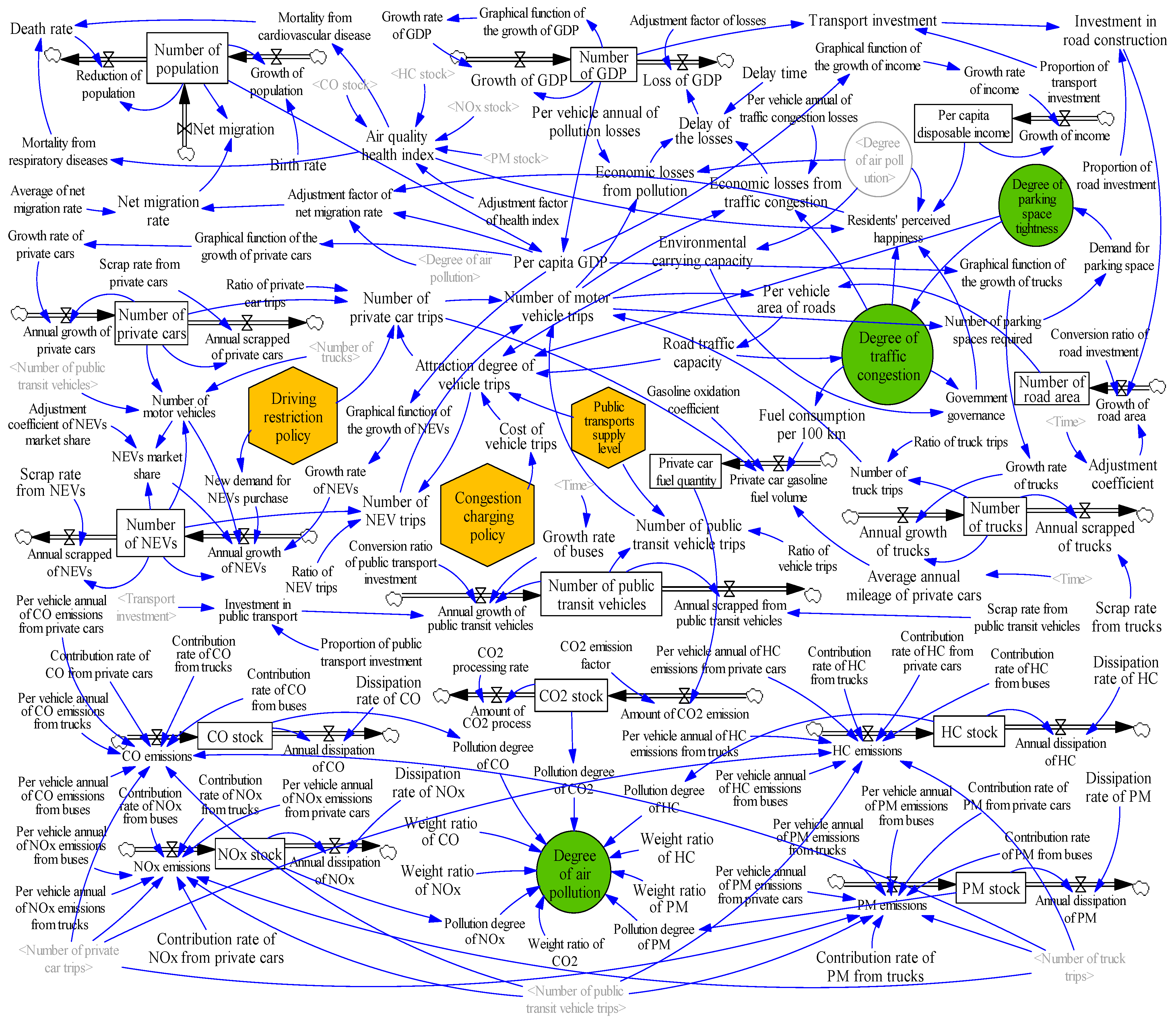
2.2.2. Stock and Flow Diagram

In SD modeling, variables are categorized into level variables, rate variables, auxiliary variables, and constants. Causal diagrams cannot differentiate between these variable types. Therefore, the model is further quantified. Based on causality analysis, VENSIM software is used to establish a stock flow diagram of the urban CMPC management model, as shown in Figure 3. The model comprises 14 level variables, 26 rate variables, 85 auxiliary variables, and 54 constants. Model setting: initial time = 2010; final time = 2035; time step = 1; unit of time: year.

The assumptions of the model are as follows:

Assumption 1:

Under the driving-restriction policy, when the number of restricted license plate endings is a, about a × 10% of vehicle trips will be reduced, excluding vehicles not subject to the restriction (e.g., NEVs).

Assumption 2:

In the environmental subsystem, the primary pollutants emitted by fuel vehicles include CO, HC, NOx, and PM [5]. Meanwhile, considering that private cars account for about 11% of global CO₂ emissions, representing the largest share within the transportation sector [50], we selected CO, HC, NOx, PM, and CO₂ emissions as key indicators to evaluate urban traffic pollution.

Assumption 3:

In the social subsystem, private cars mainly refer to fossil-fuel vehicles with exhaust emissions. Since NEVs produce zero emissions during operation, they do not emit pollutants in the model. Pollution and energy consumption in other stages of the NEV life cycle (e.g., battery production and recycling) are not considered in this study for the time being.

Assumption 4:

The public transportation in the model refers to the overall public transportation system of the city, including buses and urban rail transit.

2.3. Data Sources

2.3.1. Determination of Main Parameters and Equations

Based on the above model, this study takes Beijing as an example for simulation analysis. China has consistently ranked first globally in NEV production and sales for multiple years, and Beijing, as the nation’s capital and a pioneer in NEV promotion, offers significant advantages in policy implementation effect, data integrity, and representation. Selecting Beijing as the case study not only validates the model’s applicability but also provides valuable reference for other cities. Data mainly come from the Beijing Statistical Yearbooks (2011–2024), China Statistical Yearbooks (2011–2024), Ministry of Ecology and Environment (MEE) of the People’s Republic of China (2011–2023), Beijing Transport Development Annual Report (Beijing Transport institute, 2019–2024), and the existing literature. Some parameters and initial values of the model are shown in

Table 1. Some parameters and initial values of the model.

Variable	Value	Unit	Data sources
Urban GDP	1.4964 × 1012	yuan	Beijing Statistical Yearbooks (2011–2024)
Number of population	1.9619 × 107	person
Number of private cars	3.7151 × 106	vehicle
Number of road area	9.3950 × 107	m2
Birth rate	0.0080	1/year
Death rate	0.0049	1/year
Average of net migration rate	0.0046	1/year
CO stock	216,923.5100	ton	Calculated by MEE [5]
HC stock	29,695.7500	ton
NOx stock	39,621.1500	ton
PM stock	2932.6800	ton
Contribution rate of CO from private cars	0.5753	—	Calculated by MEE [5] and Jia and Yan [34]
Per vehicle annual of PM emissions from trucks	0.0152	ton/(vehicle × year)
Scrap rate	0.0670	—	Yang et al. [51]
Dissipation rate	0.2000	—
Ratio of vehicle trips	0.5500	—	Jia and Yan [34]
CO2 emission coefficient	2.9251	Kg/L	Provincial Greenhouse Gas Inventory Compilation Guide (Trial)

. The determination of equations in the model is mainly based on the actual situation and related literature [34,36,48,51,52,53]. Since the level equations in the model are fixed, they are not presented here, and we mainly list the rate equations and auxiliary variable equations, as shown in

Table 2. Main equations of the model.

Equations		Number
Rate variables
Growth of population (t) (person/year) =	Number of population (t) (person) × Birth rate (1/year)	(1)
Growth of GDP (t) (yuan/year) =	Urban GDP (t) (yuan) × Growth rate of GDP (1/year).	(2)
Annual dissipation of CO (t) (ton/year) =	CO stock (t) (ton) × Dissipation rate of CO (1/year)	(3)
Loss of GDP (t) (yuan/year) =	Delay of the losses (t) (yuan) × Adjustment factor of losses (1/year)	(4)
Annual growth of private cars (t) (vehicle/year) =	Number of private cars (t) (vehicle) × Growth rate of private cars (1/year)	(5)
Private car gasoline fuel volume(t) (L/year) =	Gasoline oxidation coefficient × Fuel consumption per 100 km (L/100km) × Number of private car trips (t) (vehicle) × Average annual mileage of private cars (t) (km/(vehicle × year)) ÷ 100.	(6)
Delay of the losses (t) (yuan) =	SMOOTH (Economic losses from traffic congestion (t) (yuan) + Economic losses from pollution (t) (yuan), Delay time)	(7)
CO emissions (t) (ton/year) =	CO emissions from private cars + CO emissions from trucks + CO emissions from buses	(8)
CO emissions from private cars (t) (ton/year) =	Number of private car trips (t) (vehicle) × Contribution rate of CO from private cars × Per vehicle annual of CO emissions from private cars (ton/(vehicle × year))	(9)
CO emissions from trucks (t) (ton/year) =	Number of truck trips (t) (vehicle) × Contribution rate of CO from trucks × Per vehicle annual of CO emissions from trucks (ton/(vehicle × year))	(10)
CO emissions from buses (t) (ton/year) =	Number of bus trips (t) (vehicle) × Contribution rate of CO from buses × Per vehicle annual of CO emissions from buses (ton/(vehicle × year))	(11)
Auxiliary variables
Attraction degree of vehicle trips =	0.15 × (1+Road traffic capacity) + 0.3/LN (Cost of vehicle trips) + 0.2 × (1 − Public transports supply level) + 0.15 × (1 − Degree of parking space tightness) + 0.2 × (1+Environmental carrying capacity)	(12)
Degree of traffic congestion =	(1 − Road traffic capacity) × 0.7+Degree of parking space tightness × 0.3	(13)

.

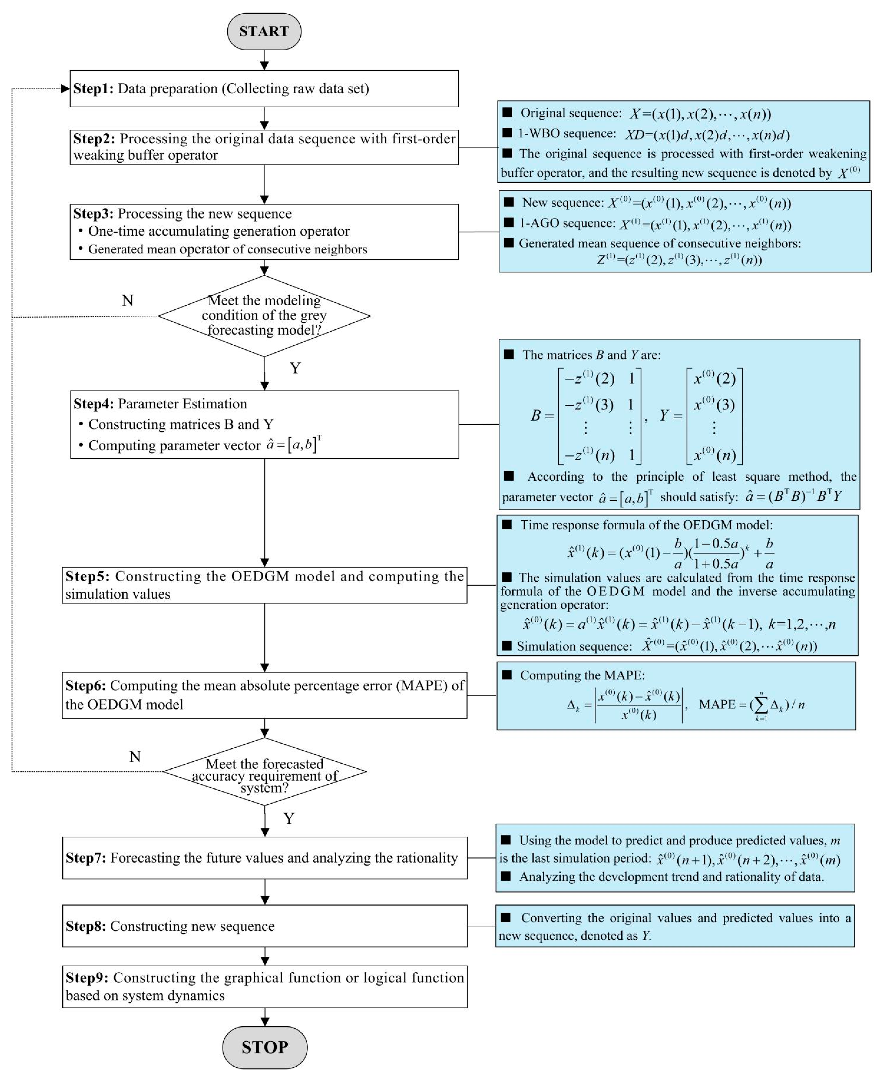
2.3.2. Determination of Auxiliary Variables Based on SD-OEDGM

Within the CMPC management model, some auxiliary variables (e.g., GDP growth rate, private car growth rate, and road traffic capacity) exhibit nonlinear characteristics, making direct establishment of correlation equations for quantification challenging. Here, we propose an integrated algorithm based on system dynamics and optimized even difference grey model (SD-OEDGM) to determine these auxiliary variables. Utilizing relevant data spanning 2010 to 2024, the methodological framework consists of three main stages: First, a first-order weakening buffer operator is applied to process the original data sequence. Second, an even difference grey model is constructed for the operator-processed sequence, enabling high-precision prediction during the simulation period. Finally, table functions and logic functions within SD are utilized to achieve more accurate descriptions of these variables.

This integrated approach not only combines the strengths of both methodologies and overcomes the deficiency of partial validation but also effectively resolves simulation and prediction problems associated with nonlinear characteristic variables. The algorithm enhances the precision of variable equation descriptions within the model, thereby improving overall model accuracy and effectiveness. The innovations of the SD-OEDGM method are as follows: (1) The integration of SD with an OEDGM establishes a bidirectional feedback mechanism that enhances adaptability to nonlinear scenarios such as policy shocks. (2) The application of a weakening buffer operator to preprocess raw data effectively smooths sudden disturbances, significantly improving the smoothness of the original data sequence. The advantages of this method are manifested in three aspects: (1) The weakening buffer operator reduces nonlinear interference, demonstrating particular robustness when handling variables affected by policy shocks (e.g., GDP growth rate). (2) The structured integration enables sophisticated nonlinear relationship modeling. The two-stage processing of “buffer operator preprocessing + SD function” effectively balances short-term fluctuations with long-term trends. The integration of grey prediction results with SD table functions achieves more accurate long-term trend capture. (3) Model optimization enhances prediction accuracy. While traditional grey models (e.g., GM (1,1)) show limited fitting capability for highly volatile nonlinear data, OEDGM improves trend-change detection through even difference optimization, making it particularly suitable for nonlinear variable modeling in small-sample, data-poor scenarios.

While preserving the computational simplicity and small-sample adaptability characteristic of grey models, this method combines SD’s systematic modeling capability to deliver higher stability and reliability in nonlinear analysis for policy simulation, economic forecasting, and related applications. The algorithm flowchart is shown in Figure 4. Taking the GDP of Beijing as an example, the specific steps are shown in Appendix A.

2.4. Model Test and Validation

2.4.1. Realistic Test

The purpose of model testing is to verify whether the structural behavior of the model aligns with reality. As shown in Figure 5, with the increase in traffic restriction intensity, the number of motor vehicle trips decreases during the initial period (2010–2024), and the road traffic capacity improves. This indicates that the traffic driving restriction policy can effectively reduce vehicle trips, enhance road traffic capacity, and alleviate traffic burdens in the short term. The simulation results are consistent with reality.

However, in the long term (after 2024), especially after the implementation of the odd–even license plate policy, the number of private car trips significantly decreases, while the number of NEV trips sharply increases. This leads to a substantial rise in the number of motor vehicle trips and a rapid decline in road traffic capacity. This phenomenon occurs because the driving restriction policy primarily targets fuel-powered vehicles without imposing limits on NEVs, thereby increasing the demand for NEV purchases and trips. Consequently, a “rebound effect” in urban traffic is observed.

2.4.2. Model Validation

In order to ensure model rationality and validity, this study selected the main variables to carry out the mean square error ratio (MSER) qualified test and the small error probability qualification test. Both methods evaluate model accuracy through residual analysis [54]. The selection of MSER is based on the following considerations: First, its normalized error ratio provides dimensionless evaluation, overcoming scale-dependency issues when comparing heterogeneous variables. Second, MSER is more effective for assessing systemic behaviors where relative error magnitude matters more than absolute values. The MSER compares modeling errors with benchmark errors through normalization processing, which is suitable for the lateral accuracy comparison of variables of different dimensions. This characteristic aligns perfectly with our research context involving multi-scale sustainability indicators. The small error probability test focuses on the concentration degree of residual distribution, effectively identifying the model’s capability to capture subtle fluctuations in the system. The combination of the two not only avoids the evaluation bias that may be caused by a single index (for example, MSER is sensitive to extreme values and small error probability is sensitive to the overall distribution) but also conforms to the verification principle of “equal emphasis on macro precision and micro stability” in complex system modeling. Through the joint validation of these two methods, this study ensures the model demonstrates robust reliability across different evaluation criteria [40].

Definition 1.

[40]. Assume the original sequence is denoted as $X^{(0)}$, and its simulated value sequence and residual sequence are denoted as ${\widehat{X}}^{(0)}$ and ${\epsilon }^{(0)}$, respectively.

Then, the mean and variance of the original sequence $X^{(0)}$ can be obtained:

$$\overline{x}={\displaystyle \frac{1}{n}}{\displaystyle \sum _{k=1}^n{x}^{(0)}(k), S_1^2=}{\displaystyle \frac{1}{n}}{\displaystyle \sum _{k=1}^n{\left[x^{(0)}(k)-\overline{x}\right]}^2}$$

(14)

The mean and variance of the residual sequence ${\epsilon }^{(0)}$ can also be obtained:

$$\overline{\epsilon }={\displaystyle \frac{1}{n}}{\displaystyle \sum _{k=1}^n\epsilon (k), S_2^2=}{\displaystyle \frac{1}{n}}{\displaystyle \sum _{k=1}^n{\left[\epsilon (k)-\overline{\epsilon }\right]}^2}$$

(15)

(1) $C=S_2/S_1$ is called the mean square error ratio. For a given $C_0>0$, when $C<C_0$, the model is defined as a mean square error ratio qualified model.

(2) $p=P(\left|\epsilon (k)-\overline{\epsilon }\right|<0.6745S_1)$ is called the small error probability. For a given $p_0>0$, when $p<p_0$, the model is defined as a small error probability qualified model.

The accuracy of both models is judged by residual error. Specifically, the smaller the $C$, the better. Because a smaller $C$ value indicates smaller $S_2$ (residual variance) and larger $S_1$ (original data variance), meaning the residuals are more concentrated with smaller fluctuations while the original data shows greater dispersion with larger variations. Therefore, superior modeling performance requires $S_2$ to be as small as possible relative to $S_1$. For any given set of $C_0$ and $p_0$ values, the model’s accuracy grade can be determined accordingly. The accuracy test grade is shown in

Table 3. Reference list of accuracy test grade.

Accuracy Grade	Grade 1	Grade 2	Grade 3	Grade 4
Mean square error ratio	0.3500	0.5000	0.6500	0.8000
Small error probability	0.9500	0.8000	0.7000	0.6000

.

Here, taking the number of private cars as an example, the historical and simulated values from 2010 to 2023 were used for the mean square error ratio and small error probability qualified test. Its original and simulated sequences are recorded as $X^{(0)}$ and ${\widehat{X}}^{(0)}$, respectively. Then,

$$X^{(0)}=\left[\begin{array}{l}{x}^{(0)}(2010)\\ x^{(0)}(2011)\\ \hfill ⋮\hfill \\ x^{(0)}(2023)\end{array}\right]=\left[\begin{array}{l}\mathrm{3,715,100}\\ \mathrm{3,872,900}\\ \mathrm{4,055,500}\\ \hfill ⋮\hfill \\ \mathrm{5,235,200}\\ \mathrm{5,348,800}\\ \mathrm{5,431,000}\end{array}\right], {\widehat{X}}^{(0)}=\left[\begin{array}{l}{\widehat{x}}^{(0)}(2010)\\ {\widehat{x}}^{(0)}(2011)\\ \hfill ⋮\hfill \\ {\widehat{x}}^{(0)}(2023)\end{array}\right]=\left[\begin{array}{l}\mathrm{3,715,100}\\ \mathrm{3,877,760}\\ \mathrm{4,065,870}\\ \hfill ⋮\hfill \\ \mathrm{5,310,190}\\ \mathrm{5,435,890}\\ \mathrm{5,560,230}\end{array}\right]$$

Firstly, the mean and variance of the original sequence can be calculated as

$$\overline{x}={\displaystyle \frac{1}{14}}{\displaystyle \sum _{k=2010}^{2023}{x}^{(0)}(k)\approx \mathrm{4,619,400}, S_1^2=}{\displaystyle \frac{1}{14}}{\displaystyle \sum _{k=2010}^{2023}{\left[x^{(0)}(k)-{\overline{x}}^{(0)}\right]}^2=2.7753\times {10}^{11}}.$$

Secondly, the residual error sequence can be calculated as

$${\epsilon }^{(0)}=\left[\begin{array}{l}\epsilon (2010)\\ \epsilon (2011)\\ \hfill ⋮\hfill \\ \epsilon (2023)\end{array}\right]=\left[\begin{array}{l}{x}^{(0)}(2010)-{\widehat{x}}^{(0)}(2010)\\ x^{(0)}(2011)-{\widehat{x}}^{(0)}(2011)\\ \hfill ⋮\hfill \\ x^{(0)}(2023)-{\widehat{x}}^{(0)}(2023)\end{array}\right]=\left[\begin{array}{l}0\\ -4860\\ -\mathrm{10,370}\\ \hfill ⋮\hfill \\ -\mathrm{74,990}\\ -\mathrm{87,090}\\ -\mathrm{129,230}\end{array}\right]$$

Similarly, the mean and variance of the residual sequence can be calculated as

$$\overline{\epsilon }={\displaystyle \frac{1}{14}}{\displaystyle \sum _{k=2010}^{2023}\epsilon (k)\approx -\mathrm{24,937},S_2^2=}{\displaystyle \frac{1}{14}}{\displaystyle \sum _{k=2010}^{2023}{\left[\epsilon (k)-\overline{\epsilon }\right]}^2\approx \mathrm{2,389,717,949}.}$$

Finally, for a given $C_0=0.3500$, $C=S_2/S_1\approx 0.0928<0.3500=C_0$. According to Definition 1 and Table 3, the accuracy belongs to grade 1.

For a given $p_0=0.9500$, $p=P(\left|\epsilon (k)-\overline{\epsilon }\right|<0.6745S_1)=1>0.9500=p_0$. According to Definition 1 and Table 3, the accuracy also belongs to grade 1.

The same method can be used to test the urban population and number of trucks from 2010 to 2022, and the accuracy all belongs to grade 1. Therefore, the model has high precision and can be used for prediction analysis.

3. Results

3.1. Green Paradox Effect of NEV Promotion Policy

In order to promote NEV adoption, some cities in China have implemented a series of incentives, such as traffic driving restrictions for fuel-powered vehicles while exempting NEVs. Currently, Beijing’s traffic restriction policy is double-tail number restriction per working day on roads within the Fifth Ring Road (excluding the Fifth Ring Road) [55]. In cases of severe congestion or pollution, the city enforces odd–even number restrictions [56].

To systematically evaluate the “green paradox” effect under different restriction intensities, we adopt a static policy assumption (i.e., fixed restriction levels post-implementation), following the approach used in prior studies [23,57]. This static assumption aligns with Beijing’s policy implementation. This approach isolates the immediate impact of each policy scenario without confounding from dynamic adjustments, enabling a clear comparison between: Scenario 1 (Baseline): No restrictions; Scenario 2 (Routine Policy): Double-tail restriction (20% of vehicles are restricted, consistent with Beijing’s current policy), reflecting daily implementation; and Scenario 3 (Emergency Policy): Odd–even restriction (50% of vehicles are restricted), representing severe conditions. By adjusting the model parameters, the three scenarios were simulated to analyze changing trends of main variables. The simulation results are displayed in Figure 6 and

Table 4. Influence of the major variables under different scenarios (in 2035).

Variables	Scenario1	Scenario2	Variation	Scenario3	Variation
NEV market share (Dmnl)	0.1611	0.2971	84.46%	0.4686	190.94%
Degree of traffic congestion (Dmnl)	0.7295	0.7573	3.81%	0.8324	14.11%
Degree of parking space tightness (Dmnl)	0.6613	0.7183	8.63%	0.8573	29.64%
Fuel consumption per 100 km (L)	9.5593	9.7331	1.82%	10.2027	6.73%
CO stock (Ton)	1,296,450	1,138,820	−12.16%	959,307	−26.01%
Degree of air pollution (Dmnl)	0.6066	0.5342	−11.94%	0.4522	−25.46%

.

Figure 6a shows that the NEVs market share gradually increases with the intensification of traffic restrictions. Compared to scenario 1, the NEV market share in scenarios 2 and 3 increases by 84.46% and 190.94%, respectively (Table 4). This may be attributed to the lower energy costs and unrestricted usage of NEVs, which stimulate new demand for NEV purchase among some commuters (from a long-term perspective). Figure 6b and Table 4 reveal that curves 2 and 3 initially fall below curve 1 but rise sharply and surpass it after 2025, increasing by approximately 3.81% and 14.11% by 2035. Similarly, the degree of parking space tightness increases by 8.63% and 29.64% (Figure 6c). These results indicate that traffic restriction has a positive effect on alleviating congestion in the short term, but the effectiveness diminishes over time. The policy promotes the replacement of fuel vehicles by NEVs, increasing the number of NEV trips (Figure 5d) and motor vehicle trips (Figure 5a), thereby generating new congestion and parking demand. In terms of pollution reduction, Figure 6e shows that with the intensity of driving restrictions and the increase in NEV market share, although the CO stock has decreased (~12.16% and ~26.01%), the overall trend is still rising, which indicates that pollution issues are not fundamentally resolved. This may be due to new congestion causing frequent deceleration and braking, increasing fuel consumption per 100 km for fuel-powered vehicles (Figure 6d), thereby raising exhaust emissions and air pollution.

The simulation results above suggest that the NEV promotion policy may trigger a “green paradox” effect. Below, we further explore the underlying mechanisms from technical perspectives by integrating traffic flow theory and vehicle emission models: (1) Macroscopic traffic flow theory focuses on vehicle density and average speed [58]. While the NEV promotion policy (e.g., driving restrictions) may alleviate congestion in the short term, it stimulates NEV purchases and usage demand in the long run, leading to increased vehicle trips (Figure 5). When traffic density exceeds road network capacity, the traffic state undergoes a significant transition. Vehicles frequently decelerate and brake, resulting in stop-and-go conditions. Once capacity is reached, further increases in vehicle density push traffic flow into an unstable state [59]. In highly saturated traffic, hard braking can trigger a chain reaction, causing traffic breakdowns [58]. This explains why, as NEV numbers rise, the road network shifts from free-flow to congested conditions, potentially reaching full congestion—where vehicle spacing minimizes, and both density and speed drop to their lowest levels. (2) Vehicle emission models are used to accurately estimate road traffic emissions, with significant variations in emissions across different driving states [60]. Under congested conditions, frequent acceleration and deceleration lead to higher per-mile emissions from fuel-powered vehicles compared to steady-speed driving [49]. Although NEVs produce zero tailpipe emissions, they indirectly increase additional emissions from fuel vehicles by altering overall traffic flow status. In summary, NEV promotion policies exert influence on both traffic flow and vehicle emissions, with these two factors interacting to generate compounded effects on traffic congestion and pollution. From a long-term perspective, policy implementation may lead to increased road vehicle density and traffic flow instability, which in turn affects the emission efficiency of conventional fuel vehicles, ultimately triggering the “green paradox” effect. This mechanism provides a comprehensive explanation for the observed trends of worsening congestion and increasing pollution in the simulation results (Figure 6).

3.2. Policy Optimization Analysis

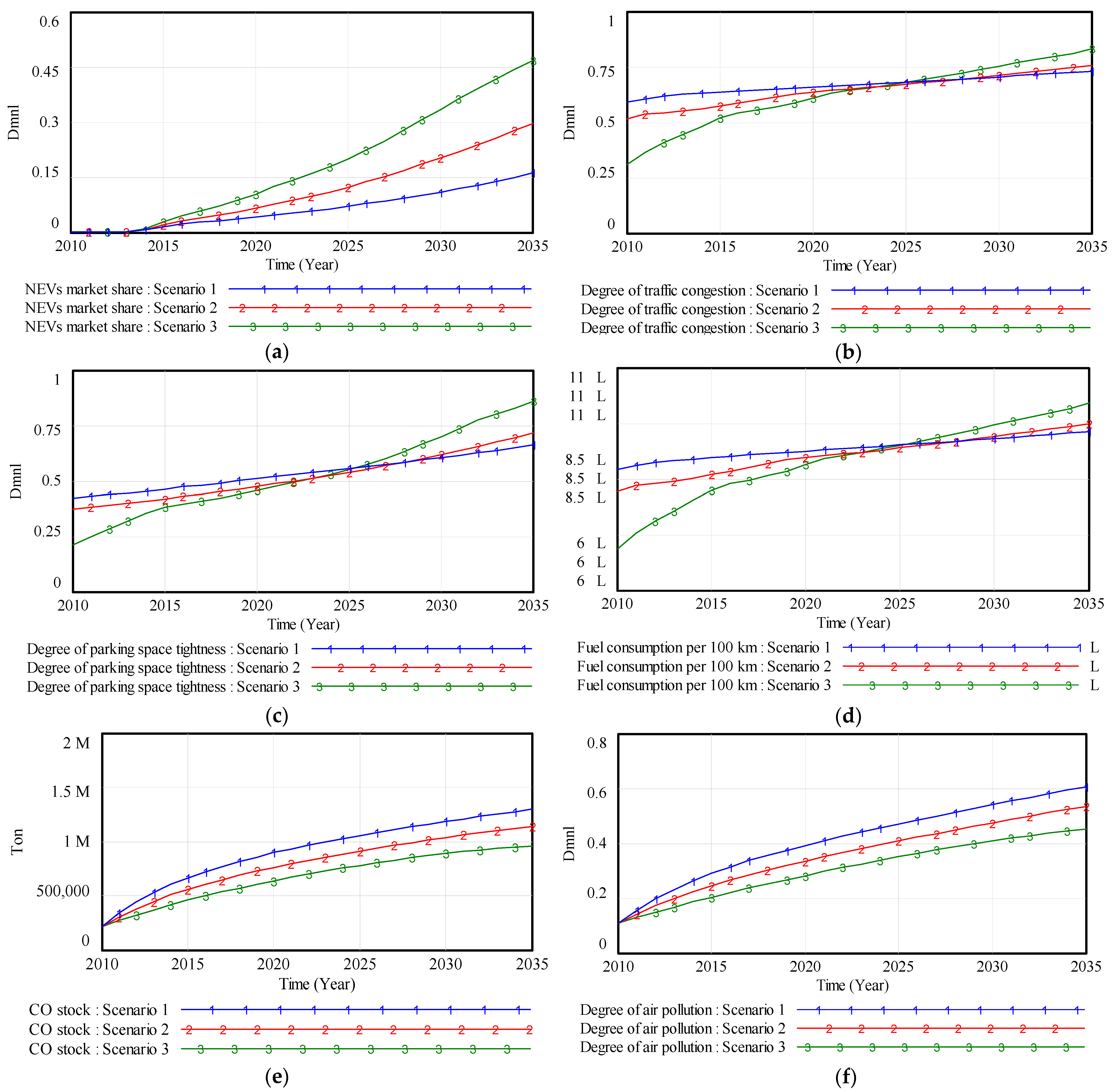
3.2.1. Scenario Simulation

In view of the “green paradox” effect of the above policy, the strategies of the congestion charging policy (CCP) and improving public transport supply level (IPTSL) were introduced. See

Table 5. Policy optimization scenario design and description.

Scenarios	Detailed Description
BS	Baseline Scenario (BS) mainly refers to the double-tail number restriction policy currently implemented in Beijing.
BS + CCP	Based on the baseline scenario, CCP is introduced to increase the cost of vehicle trips and reduce the total amount of vehicle travel. According to the existing literature [34], the charge is tentatively set at 15 yuan/(day × vehicle).
BS + CCP + IPTSL	The combination scenario builds on the promotion of NEVs and the introduction of the CCP, aiming to enhance the public transport supply level and guide the public to shift their travel modes towards green travel (with an effect of 20% [36]).

for scenario design and description. The simulation results are shown in Figure 7 and

Table 6. Comparative analysis of different scenarios (in 2035).

Variables	BS	BS + CCP	Variation	BS + CCP + IPTSL	Variation
Number of motor vehicle trips (Million vehicle)	3.3456 × 106	2.2856 × 106	−31.68%	1.8192 × 106	−45.62%
Degree of traffic congestion (Dmnl)	0.6726	0.5408	−19.61%	0.4420	−34.29%
CO stock (Ton)	1.0219 × 106	6.2238 × 105	−39.10%	4.7217 × 105	−53.79%
Degree of air pollution (Dmnl)	0.4797	0.2925	−39.02%	0.2224	−53.64%

.

In terms of alleviating traffic congestion (Figure 7a,b), Table 6 shows that compared to BS, the number of motor vehicle trips decreases by 31.68% and 45.62% under the other two scenarios, respectively, and the DTC decreases by 19.61% and 34.29%, respectively. The introduction of CCP initially controls the growth rate of curves in the early and middle stages, but a “rebound effect” is observed in the later stage (after 2027). This phenomenon may be attributed to the sunk cost effect and loss aversion effect (Chen et al., 2022) [36], which influence the number of vehicle trips and subsequently negatively impact traffic. However, when combined with an improved public transport supply level, which encourages a shift to green travel modes, the DTC shows a declining trend after a certain period. Specifically, under the combined scenario, the DTC is controlled in the early stage (2010–2017); declines rapidly in the middle stage (2017–2027), demonstrating the effectiveness of this strategy; and remains relatively stable in the later stage (after 2027).

In terms of controlling pollution (Figure 7c,d), under the BS, CO stock and DAP continues to increase; while for the other two scenarios, the growth rate of curves slows down. Compared with BS, CO stock decreases by 39.10% and 53.79% under the other two scenarios, respectively, and the DAP decreases by 39.02% and 53.64%, respectively (Table 6). The combined scenario demonstrates better emission reduction effects. In the early stage of policy implementation (2010–2017), the pollution control effect is not significant, with CO stock and DAP continuing to rise. During the middle simulation stage (2017–2027), the curves remain relatively stable, indicating that pollutant emissions are controlled as the policies are implemented and improved. After about 2027, both CO stock and DAP show a declining trend, highlighting the effectiveness of this strategy.

These results indicate that the combination scenario can absorb the advantages of both strategies and effectively weaken the paradox effect. It can not only alleviate traffic congestion (Figure 7a,b) but also effectively reduce pollutant emissions (Figure 7c), achieving the goal of pollution control (Figure 7d).

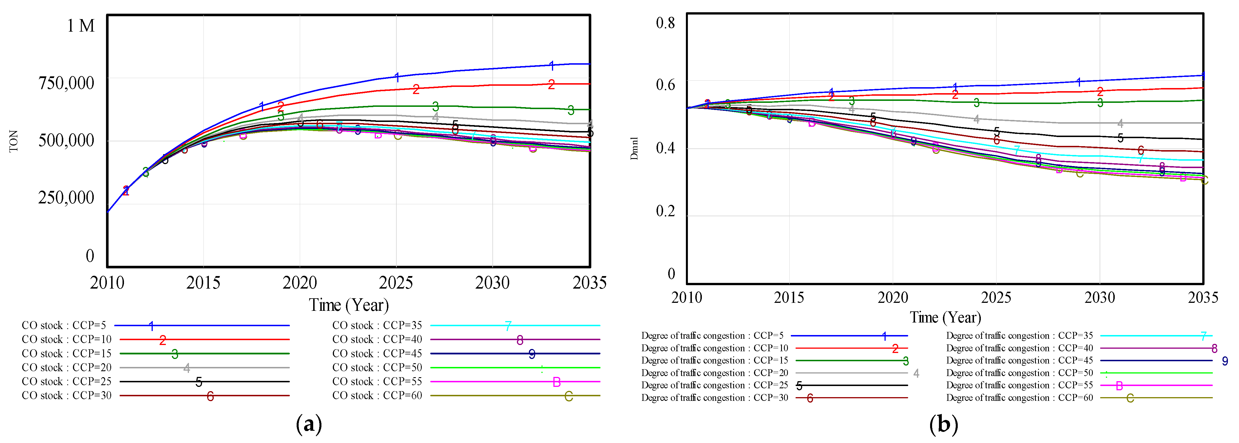
3.2.2. Sensitivity Analysis

To determine the reasonable range of CCP, a sensitivity trend analysis was conducted by adjusting model parameters. As can be seen from Figure 8a, the CO stock is minimized when the CCP is equal to 100 yuan/(day × vehicle), while it reaches its maximum when the CCP is 10 yuan/(day × vehicle). These results are consistent with reality. In addition, in the horizontal direction, although the growth rate of curve 1 declines over time, the CO stock continuously rises. Therefore, pollution control cannot be realized when the CCP is 10 yuan/(day × vehicle). However, the other curves initially rise and then decline, indicating that the CCP can reduce pollutant emissions after a certain period of implementation, achieving pollution control. In the longitudinal direction, the CO stock declines with the increase in CCP. In particular, the gap between curves 2 and 6 gradually decreases, exhibiting a diminishing marginal effect. When the CCP exceeds 60 yuan, the curves show almost no change. Therefore, the CCP should be controlled within 60 yuan. The analysis of Figure 8b is similar. Further analysis is provided in Figure 9a,b and

Table 7. The influence of CO stock and degree of traffic congestion under different CCP (in 2035).

CCP	CO Stock (Ton)	Variation	Degree of Traffic Congestion (Dmnl)	Variation
5	804,408	—	0.6156	—
10	723,608	−10.04%	0.5780	−6.11%
15	622,380	−13.99%	0.5408	−6.44%
20	565,134	−9.20%	0.4747	−12.22%
25	532,400	−5.79%	0.4273	−9.98%
30	509,270	−4.34%	0.3894	−8.86%
35	490,895	−3.61%	0.3631	−6.76%
40	476,820	−2.87%	0.3417	−5.89%
45	472,128	−0.98%	0.3241	−5.15%
50	468,965	−0.67%	0.3165	−2.34%
55	466,864	−0.45%	0.3108	−1.81%
60	465,076	−0.38%	0.3064	−1.40%

.

As shown in Figure 9a,b and Table 7, the CO stock decreases with the increase in CCP, and the gap between curves initially widens and then gradually narrows. Among them, the most significant changes occur in the range of [5,15], with change rates of -10.04% and −13.99%, respectively. In the interval of [15,40], the curve changes gradually slow down, with only a 2.87% decrease in the interval of [35,40]. However, the curves almost overlap when CCP is larger than 40 yuan. Therefore, from a pollution control perspective, the CCP should be located in the interval of [15,40]. Similarly, the congestion alleviation effect gradually increases in the interval of [5,20], with change rates of 6.11%, 6.44%, and 12.22%. Notably, when the CCP is 15 yuan, congestion is slightly alleviated in the middle stage but shows a “rebound effect” in the later stage (after 2027). The most significant congestion alleviation effects occur in the range of [15,20], with improved congestion conditions in the later stage. However, the gap between curves gradually decreases in the range of [20,45], and the curves have remained almost unchanged when CCP exceeds 45 yuan. Therefore, from a congestion alleviation perspective, the CCP should fall within the interval of [20,45]. In summary, considering both congestion alleviation and pollution control, the reasonable range of CCP is 20–40 yuan/ (day × vehicle).

4. Discussion

The substitution of fuel vehicles by NEVs is an effective measure to reduce pollutant emissions since they are clean and efficient, and their energy can be provided by renewable energy sources (e.g., wind energy or solar energy) [32]. Hence, many countries have introduced a series of incentives (such as no restrictions on driving) to promote the adoption of NEVs. Studies have shown that as the intensity of traffic restrictions increases, the NEV market share rises, which contributes to alleviating traffic-related pollution. However, in the long term, this may exacerbate congestion and parking demands, leading to side effects, which are consistent with the findings of the existing literature [32,47,48,61]. Considering the extra traffic congestion, Wang et al. [32] proposed implementing some interventions, such as CCP, to alleviate the side effect and achieve more benefits. Although CCP can alleviate congestion and reduce pollution, some travelers will turn to public transportation, thus increasing the burden of public transportation, so it is necessary to improve the supply level of public transportation [34]. By optimizing an urban travel system, the shifting of travel mode from private car to bus and metro can effectively alleviate road congestion and reduce CO₂ emissions [62]. The long-term effects of these policies on traffic and the environment warrant further exploration.

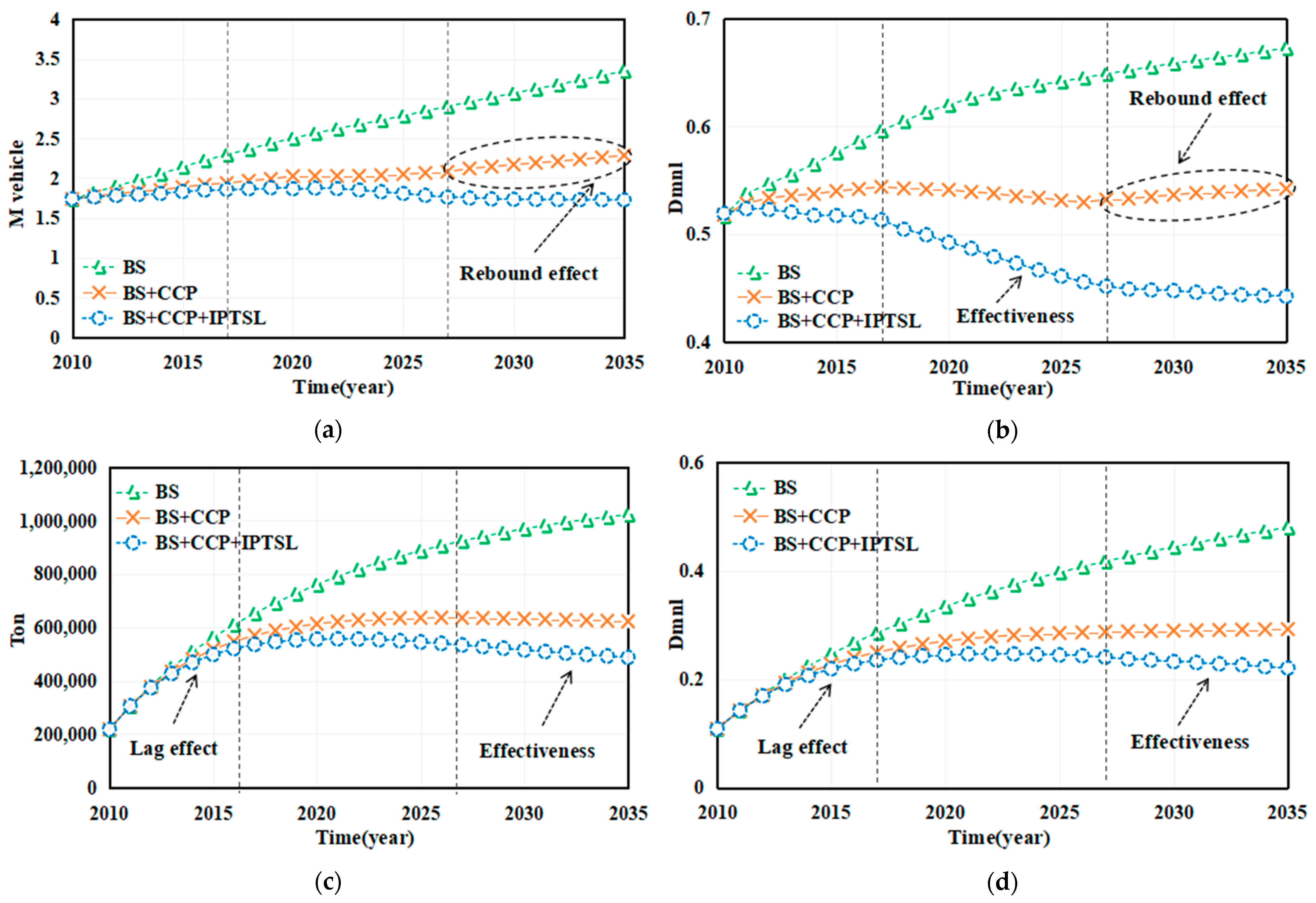
4.1. Rebound Effect and Lag Effect

A traffic driving restriction policy, as a non-economic incentive, promotes the substitution of conventional fuel vehicles with NEVs, accelerating the “substitution effect” and increasing the NEV market share (Figure 6a). The reason for this may be that the restrictions primarily target fuel vehicles, prompting some travelers with higher incomes or lower environmental awareness to purchase a second vehicle or travel multiple times. Residents in large cities prioritize travel convenience, and the exemption of NEVs from driving restrictions, coupled with relaxed purchase restriction policy, may stimulate new demand for vehicle purchase. The increase in NEV market share positively impacts the reduction of vehicle exhaust emissions. However, in the long term, as the NEV market share rises, the number of motor vehicle trips gradually increases (Figure 5a), leading to a “rebound effect” in traffic congestion (Figure 6b), which reflects the “green paradox effect.” From a life-cycle perspective, NEVs produce zero emissions during operation, but the production and recycling of batteries generate pollutants, resulting in a risk of environmental pollution transfer [12,61]. New congestion may slow down vehicles, increasing fuel consumption per 100 km and exhaust emissions of fuel vehicles, thereby affecting air quality. Therefore, when implementing the traffic restriction policy, the transport department should scientifically and flexibly adjust the policy’s intensity and targets based on regional development and actual conditions.

According to Jia et al. [63], CCP should not exceed 100 yuan, as higher charging is not better. When the CCP is 15 yuan/(day × vehicle), DTC is moderately controlled in the early and middle stages, but a “rebound effect” occurs in the later stages (Figure 7a,b), which is similar to the findings of Jia and Yan [34] and Chen et al. [36]. This phenomenon may be attributed to the sunk cost and loss aversion effects, which influence the number of vehicle trips and subsequently exacerbate DTC. Sensitivity analysis indicated that the reasonable range of CCP is 20–40 yuan/(day × vehicle). The implementation of CCP is inseparable from the improvement of the public transport system, so it is necessary to improve the supply level of public transportation and guide residents to travel green while implementing CCP. By improving the public transport supply level, it is found that the combination scenario has a “lag effect” in the early stage (Figure 7c,d) and shows effectiveness in the middle stage (in terms of congestion mitigation) and the later stage (in terms of pollution control).

In addition, the actual emission reduction effect of the above policies also depends on the technological differences among NEVs. The impact of different NEV technologies on the “green paradox” is significantly different, and their emission reduction effects are highly dependent on technical characteristics and energy structure synergy [64]: While BEVs have a high energy conversion efficiency, their actual emission reduction benefits are related to grid cleanliness [25]; PHEV emissions are significantly influenced by user charging behavior; in regions with limited charging infrastructure availability, they may degrade into conventional hybrid mode. FCEVs can only achieve near-zero emissions when fully powered by green hydrogen, yet they face dual potential constraints of high production costs and underdeveloped refueling infrastructure [10]. This demands a multi-dimensional priority assessment framework for policy-making: (1) In terms of technical efficiency: Prioritize BEV promotion in regions with mature power infrastructure; (2) In terms of regional resource endowment: Explore sodium-ion battery alternatives in lithium-scarce areas, while piloting FCEVs in hydrogen-abundant regions [65]; (3) In terms of energy system synergy: Transition with PHEVs in grid-constrained regions, and couple FCEV development with green hydrogen production [66]. It should be emphasized that any NEV promotion strategy decoupled from regional energy restructuring could shift pollution from tailpipe emissions to power generation—potentially exacerbating rather than mitigating the “green paradox” effect. This potential constraint is particularly prominent in coal-dependent regions (e.g., India’s 70% coal-powered grid) [67]. Large-scale BEV charging could increase coal-based electricity consumption, necessitating renewable energy integration and grid upgrades to achieve genuine emission reductions [13]. Therefore, an effective NEV policy must concurrently advance infrastructure development, technological innovation, and low-carbon energy transition, forming an integrated governance framework that unifies technical feasibility, resource availability, and policy sustainability.

4.2. Synergistic Benefits of Combination Scenario

In view of the “green paradox” effect of the NEV promotion policy, we have introduced a combination scenario for policy optimization analysis. This section explores the synergistic benefits by comparing the trends of main variables under the baseline and combination scenarios (Figure 10,

Table 8. Influence of the major variables in the combination scenario (in 2035).

Variables	BS	BS + CCP + IPTSL	Variation
Degree of traffic congestion (Dmnl)	0.6726	0.4420	−34.29%
Degree of parking space tightness (Dmnl)	0.5608	0.3956	−29.45%
Road traffic capacity (Dmnl)	0.2794	0.5382	92.61%
Loss of GDP (yuan/year)	6.3906 × 109	1.2710 × 109	−80.11%
Economic losses from pollution (yuan)	8.9505 × 109	1.8849 × 109	−78.94%
Economic losses from traffic congestion (yuan)	4.1956 × 109	6.4905 × 108	−84.53%
Degree of air pollution (Dmnl)	0.4797	0.2224	−53.64%
Environmental carrying capacity (Dmnl)	0.5203	0.7708	48.14%
Air quality health index (Dmnl)	7.0064	2.9979	−57.21%

).

• Social benefit

As can be seen from Figure 10a–c and Table 8, under the combination scenario, the RTC increases from 0.2794 to 0.5382, an increase of about 92.61%. Meanwhile, the DTC and the degree of parking space tightness decrease by about 34.29% and 29.45%, respectively. These results indicate that this strategy can effectively alleviate DTC and improve RTC, which shows the social benefits of combination scenario.

• Economic benefit

Figure 10d shows that under the combination scenario, the loss of GDP initially increases, peaks in 2017, and then exhibits a declining trend. The change trend is associated with the “lag effect” of this strategy. The policy effects are unstable in the early stages but gradually appear over time. This contrasts with the effect of the traffic restriction policy, an administrative measure that yields immediate results but stimulates new car purchase demand in the long term [68,69]. Figure 10d shows that the “lag effect” increases rapidly during 2010–2017 but declines in the mid-to-late stages of policy implementation (after 2017). The results show that the continuous promotion of combination policy greatly reduces the loss of GDP (~80.11%). Similarly, Figure 10e shows the same trend. The difference is that pollution losses decline slowly in the later period, while congestion losses change significantly (Figure 10f). Compared with the baseline scenario, the economic losses from pollution and congestion in the combination scenario reduce by about 78.94% and 84.53%, respectively (Table 8).

• Environmental benefit

Figure 10g shows that DAP increases year by year under the baseline scenario, indicating limited pollution control effect. In contrast, the combination scenario shows good environmental benefits, with DAP rising initially but declining after 2027 (Figure 7d and Figure 10g), which reveals the “lag effect” of this strategy in environmental terms. Compared to the BS, under the combination scenario, DAP reduces by 52.21%, and ECC increases by 48.14% (Table 8). Such improvement points to the importance of the combination scenario in mitigating the adverse environmental impacts of vehicles.

• Health benefit

Vehicle exhaust emissions reduce air quality and harm public health. Considering the relationship between air pollution and public health, this study introduced the air quality health index (AQHI), which is linked to pollutants emitted by vehicles and affects mortality rate of residents [70]. The smaller the AQHI, the better. As shown in Figure 10i and Table 8, compared to the BS, the AQHI under the combination scenario begins to decline in 2024 and decreases by approximately 57.21% by 2035. These changes reflect the positive role of combination scenario in improving residents’ health benefits.

To sum up, on the basis of promoting NEVs, introducing CCP and improving the public transport supply level can not only achieve dual governance of congestion alleviation and pollution control but also have a positive effect on reducing economic losses and improving the health benefits of residents. Therefore, the combination scenario has certain synergistic benefits in society, economy, environment, and health.

5. Conclusions

5.1. Main Conclusions

This study uses the SD-OEDGM approach to establish an urban CMPC management model. Based on mid- and long-term dynamics analysis of NEVs promotion policy, the following conclusions were obtained:

• The integrated algorithm of SD-OEDGM fully leverages the advantages of system dynamics and grey prediction theory, overcoming the limitations of partial validation. It effectively addresses the simulation and prediction of variables with nonlinear characteristics, more accurately describes model parameters and equations, and enhances the model’s precision and validity.
• Promoting NEVs effectively reduces vehicle exhaust emissions and alleviates traffic pollution but may lead to negative effects over time. As a non-economic incentive, driving restrictions on fuel-powered vehicles while exempting NEVs may, in the long run, stimulate new vehicle demand and accelerate the “substitution effect” of NEVs, resulting in a “green paradox” effect. For instance, DTC exhibits a “rebound effect” in later stages, further increasing parking demand and fuel consumption per 100 km for conventional fuel vehicles.
• To overcome the limitations of the policy, this study introduces a combined strategy of CCP and improved public transport supply level. CCP reduces the attraction degree of vehicle trips by increasing the cost of vehicle trips, but higher charges do not necessarily yield better outcomes. From the perspectives of congestion alleviation and pollution control, the reasonable range of CCP is 20–40 yuan/(day × vehicle).
• Compared with the baseline scenario, the combination scenario can not only achieve the “win-win” of congestion alleviation (~34.29%) and pollution control (~52.21%) but also effectively reduce the degree of parking space tightness (~29.45%), decrease economic losses (~80.11%), and improve residents’ health benefits (~57.21%), which have synergistic benefits in society, economy, environment, and health. Although this strategy has a “lag effect” in the early stage, it shows effectiveness in the medium term (congestion alleviation) and long term (pollution control).

5.2. Policy Recommendations

Based on the above conclusions, the following policy recommendations are proposed:

• Develop a comprehensive traffic control plan tailored to different stages of NEV development. While NEVs can reduce traffic pollution, they may increase congestion and parking demand. Therefore, both traffic and environmental impacts need to be comprehensively considered during the transition from fuel-powered vehicles to NEVs. In the initial stage of NEV promotion, some incentives such as high subsidies and unrestricted driving have been implemented. However, as the NEV market expands, policy support intensity should be reconsidered. For example, redirect purchase subsidy to battery R&D and introduce moderate NEV driving restrictions in congested areas. Implement diversified policies, such as CCP, to achieve collaborative governance of congestion mitigation and pollution control.
• Introduce appropriate CCP to increase vehicle travel costs and encourage green travel. At the same time, formulate a scientific and reasonable fee scheme to improve the public’s acceptance of the policy.
• Improve fuel quality through technological means to reduce fuel consumption per 100 km and emission coefficients of fuel-powered vehicles. Accelerate the phase-out of high-pollution, older vehicles and provide subsidies and tax incentives for low-emission vehicle manufacturers and owners.
• Increase investment in public transportation to improve supply and service quality. The realization of urban congestion mitigation and pollution control relies on the active participation of travelers. Government should strengthen the publicity of policy implementation purposes and traffic and pollution problems and enhance citizens’ environmental consciousness. Guide travelers to shift from passive acceptance to active choice of green travel, change the way the public travels, and then achieve synergistic effects in congestion alleviation and pollution control.

5.3. Limitations and Future Work

Limitations and future research directions of this study include the following:

• This study takes Beijing as an example for simulation analysis, but the policy effects and research results may vary from region to region. In the future, we will conduct in-depth research considering the differences of policies and urban development in different urban contexts.
• This article does not separately explore pollution and energy consumption throughout the entire life cycle of NEVs, which is also an aspect that requires further exploration in this study.
• This study employs the OEDGM to predict certain auxiliary variables in the SD model, yet the following limitations remain: (1) Error accumulation in long-term forecasting: While the accumulated generating operation (AGO) mitigates randomness, prediction errors may amplify progressively during extended forecasting periods, causing deviations from actual trends; (2) Static parameter constraints: The conventional model’s fixed development coefficient and grey action quantity lack adaptability to dynamic data variations. Future enhancements could involve the following: For long-term prediction, integrating residual correction (e.g., Markov chain) or hybrid modeling (e.g., Grey-ARIMA) to suppress error propagation; For parameter adaptability, implementing rolling-window mechanisms or metaheuristic algorithms (e.g., particle swarm optimization) to dynamically adjust parameters, thereby improving the model’s capability to handle nonlinear data patterns.
• Future research could incorporate multi-objective optimization to quantify trade-offs between congestion mitigation, pollution control, and economic costs. The sensitivity analysis of CCP (Section 3.2.2) provides a basis for defining optimization boundaries, while the SD framework could be extended to integrate Pareto frontier analysis for policy combinations.

References

1. United States Environment Protection Agency (EPA): Transportation, Air Pollution, and Climate Change. 2024. Available online: https://www.epa.gov/transportation-air-pollution-and-climate-change (accessed on 20 December 2024).
2. Cao, C. Integration of ten years of daily weather, traffic, and air pollution data from Norway’s six largest cities. Sci. Data 2024, 11, 744. [Google Scholar] [CrossRef] [PubMed]
3. Dedoussi, I.C.; Eastham, S.D.; Monier, E.; Barrett, S.R. Premature mortality related to United States cross-state air pollution. Nature 2020, 578, 261–265. [Google Scholar] [CrossRef]
4. Nansai, K.; Tohno, S.; Chatani, S.; Kanemoto, K.; Kagawa, S.; Kondo, Y. Consumption in the G20 nations causes particulate air pollution resulting in two million premature deaths annually. Nat. Commun. 2021, 12, 6286. [Google Scholar] [CrossRef] [PubMed]
5. Ministry of Ecology and Environment (MEE) of the People’s Republic of China: China Mobile Source Environmental Management Annual Report (2011–2023). Available online: https://www.mee.gov.cn/ywgz/dqhjbh/ydyhjgl/202312/t20231207_1058461.shtml (accessed on 1 January 2024).
6. Li, P.; Zhang, Z. The effects of new energy vehicle subsidies on air quality: Evidence from China. Energy Econ. 2023, 120, 106624. [Google Scholar] [CrossRef]
7. Kejun, J.; Chenmin, H.; Songli, Z.; Pianpian, X.; Sha, C. Transport scenarios for China and the role of electric vehicles under global 2 °C/1.5 °C targets. Energy Econ. 2021, 103, 105172. [Google Scholar] [CrossRef]
8. Tan, R.; Tang, D.; Lin, B. Policy impact of new energy vehicles promotion on air quality in Chinese cities. Energy Policy 2018, 118, 33–40. [Google Scholar] [CrossRef]
9. Lin, B.; Wu, W. The impact of electric vehicle penetration: A recursive dynamic CGE analysis of China. Energy Econ. 2021, 94, 105086. [Google Scholar] [CrossRef]
10. Aguilar, P.; Groß, B. Battery electric vehicles and fuel cell electric vehicles, an analysis of alternative powertrains as a mean to decarbonise the transport sector. Sustain. Energy Technol. Assess. 2022, 53, 102624. [Google Scholar]
11. China Association of Automobile Manufacturers (CAAM): Brief Analysis of New Energy Vehicle Production and Sales in 2024. Available online: http://www.caam.org.cn/tjsj (accessed on 1 January 2025).
12. Song, X.C.; Deng, C.N.; Shen, P.; Qian, Y.; Xie, M.H. Environmental impact and carbon footprint analysis of pure electric vehicles based on life cycle assessment. Res. Environ. Sci. 2023, 36, 2179–2188. (In Chinese) [Google Scholar]
13. Schill, W.P.; Gerbaulet, C. Power system impacts of electric vehicles in Germany: Charging with coal or renewables? Appl. Energy 2015, 156, 185–196. [Google Scholar] [CrossRef]
14. Yu, Q.; He, B.Y.; Ma, J.; Zhu, Y. California’s zero-emission vehicle adoption brings air quality benefits yet equity gaps persist. Nat. Commun. 2023, 14, 7798. [Google Scholar] [CrossRef]
15. Muzir, N.A.Q.; Mojumder, M.R.H.; Hasanuzzaman, M.; Selvaraj, J. Challenges of electric vehicles and their prospects in Malaysia: A comprehensive review. Sustainability 2022, 14, 8320. [Google Scholar] [CrossRef]
16. Ministry of Industry and Information Technology of the People’s Republic of China (MIIT): Announcement on the Continuation and Optimization of Tax Reduction Policies for New Energy Vehicles. 2023. Available online: https://www.gov.cn/zhengce/zhengceku/202306/content_6887734.htm (accessed on 20 June 2023).
17. Yang, X.; Lin, W.; Gong, R.; Zhu, M.; Springer, C. Transport decarbonization in big cities: An integrated environmental co-benefit analysis of vehicles purchases quota-limit and new energy vehicles promotion policy in Beijing. Sust. Cities Soc. 2021, 71, 102976. [Google Scholar] [CrossRef]
18. Ercan, T.; Onat, N.C.; Keya, N.; Tatari, O.; Eluru, N.; Kucukvar, M. Autonomous electric vehicles can reduce carbon emissions and air pollution in cities. Transport. Res. Part D-Transport. Environ. 2022, 112, 103472. [Google Scholar] [CrossRef]
19. Zhang, L.; Wang, L.; Chai, J. Influence of new energy vehicle subsidy policy on emission reduction of atmospheric pollutants: A case study of Beijing, China. J. Clean Prod. 2020, 275, 124069. [Google Scholar] [CrossRef]
20. Li, J.; Jiang, M.; Li, G. Does the new energy vehicles subsidy policy decrease the carbon emissions of the urban transport industry? Evidence from Chinese cities in Yangtze River Delta. Energy 2024, 298, 131322. [Google Scholar] [CrossRef]
21. Alimujiang, A.; Jiang, P. Synergy and co-benefits of reducing CO2 and air pollutant emissions by promoting electric vehicles—A case of Shanghai. Energy Sustain Dev. 2020, 55, 181–189. [Google Scholar] [CrossRef]
22. Wu, D.; Xie, Y.; Lyu, X. The impacts of heterogeneous traffic regulation on air pollution: Evidence from China. Transport. Res. Part D-Transport. Environ. 2022, 109, 103388. [Google Scholar] [CrossRef]
23. Jia, S.W.; Li, Y.; Fang, T.H. Can driving-restriction policies alleviate traffic congestion? A case study in Beijing, China. Clean Technol. Environ. Policy 2022, 24, 2931–2946. [Google Scholar]
24. Wu, Y.; Yang, Z.; Lin, B.; Liu, H.; Wang, R.; Zhou, B.; Hao, J. Energy consumption and CO2 emission impacts of vehicle electrification in three developed regions of China. Energy Policy 2012, 48, 537–550. [Google Scholar] [CrossRef]
25. Zivin, J.S.G.; Kotchen, M.J.; Mansur, E.T. Spatial and temporal heterogeneity of marginal emissions: Implications for electric cars and other electricity-shifting policies. J. Econ. Behav. Organ. 2014, 107, 248–268. [Google Scholar] [CrossRef]
26. Holland, S.P.; Mansur, E.T.; Muller, N.Z.; Yates, A.J. Are there environmental benefits from driving electric vehicles? The importance of local factors. Am. Econ. Rev. 2016, 106, 3700–3729. [Google Scholar] [CrossRef]
27. Chen, Y.S.; Lan, L.B.; Du, Y.Q.; Wang, T.; Xu, H.B.; Chen, H. Environmental benefit and carbon reduction economic evaluation of extended range/battery electric/internal combustion engine vehicles based on life cycle assessment. Acta Sci. Circumstantiae 2023, 43, 516–527. (In Chinese) [Google Scholar]
28. Ma, S.C.; Fan, Y.; Feng, L. An evaluation of government incentives for new energy vehicles in China focusing on vehicle purchasing restrictions. Energy Policy 2017, 110, 609–618. [Google Scholar] [CrossRef]
29. Ma, S.C.; Xu, J.H.; Fan, Y. Willingness to pay and preferences for alternative incentives to EV purchase subsidies: An empirical study in China. Energy Econ. 2019, 81, 197–215. [Google Scholar] [CrossRef]
30. Wang, N.; Tang, L.; Zhang, W.; Guo, J. How to face the challenges caused by the abolishment of subsidies for electric vehicles in China? Energy 2019, 166, 359–372. [Google Scholar] [CrossRef]
31. Kong, D.; Xia, Q.; Xue, Y.; Zhao, X. Effects of multi policies on electric vehicle diffusion under subsidy policy abolishment in China: A multi-actor perspective. Appl. Energy 2020, 266, 114887. [Google Scholar] [CrossRef]
32. Wang, T.; Tang, T.Q.; Huang, H.J.; Qu, X. The adverse impact of electric vehicles on traffic congestion in the morning commute. Transp. Res. Part C-Emerg. Technol. 2021, 125, 103073. [Google Scholar] [CrossRef]
33. Ju, X.; Sun, B.; Jin, J. The Effect of New Energy Vehicle Policies on Traffic Congestion: Evidence from Beijing. Bus. Manag. Res. 2018, 7, 9–21. [Google Scholar] [CrossRef]
34. Jia, S.W.; Yan, G.L. Research on the traffic congestion charging fee model in urban areas based on SD-GM approach. Oper. Res. Manag. Sci. 2019, 28, 160–168. (In Chinese) [Google Scholar]
35. Koh, W.P.; Chin, K.K. The applicability of prospect theory in examining drivers’ trip decisions, in response to Electronic Road Pricing (ERP) rates adjustments-a study using travel data in Singapore. Transp. Res. Part A-Policy Pract. 2022, 155, 115–127. [Google Scholar] [CrossRef]
36. Chen, Z.; Li, B.; Jia, S. Dynamic evaluation of environmental-economic performance of vehicle emission reduction policy from the perspective of the loss-aversion effect. Sust. Cities Soc. 2022, 85, 104080. [Google Scholar] [CrossRef]
37. Viadero-Monasterio, F.; Meléndez-Useros, M.; Jiménez-Salas, M.; López Boada, M.J. Fault-Tolerant Robust Output-Feedback Control of a Vehicle Platoon Considering Measurement Noise and Road Disturbances. IET Intell. Transp. Syst. 2025, 19, e70007. [Google Scholar] [CrossRef]
38. Viadero-Monasterio, F.; Gutiérrez-Moizant, R.; Meléndez-Useros, M.; López Boada, M.J. Static Output Feedback Control for Vehicle Platoons with Robustness to Mass Uncertainty. Electronics 2025, 14, 139. [Google Scholar] [CrossRef]
39. Xiao, G.; Li, Z.; Sun, N.; Zhang, Y. Research on the Stability Control Strategy of High-Speed Steering Intelligent Vehicle Platooning. World Electr. Veh. J. 2024, 15, 169. [Google Scholar] [CrossRef]
40. Liu, S.F. Grey System Theory and Application; Science Press: Beijing, China, 2017. (In Chinese) [Google Scholar]
41. Wan, L.L.; Shan, Z.P.; Jiang, X.Y.; Wang, Z.; Lv, Y.Y.; Xu, S.M.; Huang, J.H. Life Cycle Prediction of Airport Operation Based on System Dynamics. Sustainability 2024, 16, 9596. [Google Scholar] [CrossRef]
42. Armenia, S.; Barnabé, F.; Franco, E.; Iandolo, F.; Pompei, A.; Tsaples, G. Identifying policy options and responses to water management issues through System Dynamics and fsQCA. Technol. Forecast. Soc. Change 2023, 194, 122737. [Google Scholar] [CrossRef]
43. Gao, X.J.; Zhu, A.S.; Yu, Q.F. Exploring the Carbon Abatement Strategies in Shipping Using System Dynamics Approach. Sustainability 2023, 15, 13907. [Google Scholar] [CrossRef]
44. Aftabi, N.; Moradi, N.; Mahroo, F.; Kianfar, F. Sd-abm-ism: An integrated system dynamics and agent-based modeling framework for information security management in complex information systems with multi-actor threat dynamics. Expert Syst. Appl. 2025, 263, 125681. [Google Scholar] [CrossRef]
45. Wang, W.B.; Liu, Y.; Zhong, L.S.; Qi, J.Y.; Tong, P. Research on recovery decision of waste power battery under subsidy-penalty policy. Chin. J. Manag. Sci. 2023, 31, 90–102. (In Chinese) [Google Scholar]
46. Yao, X.; Ma, S.; Bai, Y.; Jia, N. When are new energy vehicle incentives effective? Empirical evidence from 88 pilot cities in China. Transp. Res. Part A Policy Pract. 2022, 165, 207–224. [Google Scholar] [CrossRef]
47. Zhang, H.R.; Liu, Y.; Tan, X.J.; Qi, Y.; Yang, L.Y.; Jia, M.Q. Research on the impact of leap-forward development of new energy vehicles on urban traffic congestion. Chin. J. Manag. Sci. 2024, 1–19. (In Chinese) [Google Scholar]
48. Jia, S.; Bi, L.; Zhu, W.; Fang, T. System dynamics modeling for improving the policy effect of traffic energy consumption and CO2 emissions. Sust. Cities Soc. 2023, 90, 104398. [Google Scholar] [CrossRef]
49. Zhang, W.H.; Ye, M.R.; Xi, C.; Song, Z.W. Vehicle formation and carbon emission characteristics in mixed traffic flow environment. J. Jilin Univ. (Eng. Technol. Ed.) 2025, 2025, 1–12. (In Chinese). Available online: https://link.cnki.net/doi/10.13229/j.cnki.jdxbgxb.20240775 (accessed on 10 March 2025).
50. Andor, M.A.; Gerster, A.; Gillingham, K.T.; Horvath, M. Running a car costs much more than people think—Stalling the uptake of green travel. Nature 2020, 580, 453–455. [Google Scholar] [CrossRef]
51. Yang, H.X.; Li, J.D.; Zhang, H.; Liu, S.Q. Research on the governance of urban traffic jam based on system dynamics. Syst. Eng-Theor Pract. 2014, 34, 2135–2143. (In Chinese) [Google Scholar]
52. Jia, S.W. Double Dividend Effect of Vehicle Pollutant Reduction Control Strategy. Manag. Rev. 2022, 34, 53–61+182. (In Chinese) [Google Scholar]
53. Chen, Z.; Ye, X.Y.; Li, B.; Jia, S.W. Effect of Driving-Restriction Policies Based on System Dynamics, the Back Propagation Neural Network, and Gray System Theory. Arab. J. Sci. Eng. 2023, 48, 7109–7125. [Google Scholar] [CrossRef]
54. Yuan, G.D. Research on the evolution characteristics of internet public opinion crisis and its early warning scheme. J. Mod. Inf. 2021, 41, 154–159. (In Chinese) [Google Scholar]
55. Beijing Municipal Government: Notice on Implementing Traffic Restriction Measures During Peak Hours on Workdays. 2025. Available online: https://www.beijing.gov.cn/zhengce/zhengcefagui/202503/t20250324_4041745.html (accessed on 10 March 2025).
56. Beijing Traffic Management Bureau: Announcement on Temporary Traffic Control Measures for Heavy Air Pollution. 2023. Available online: https://jtgl.beijing.gov.cn/jgj/jgxx/gsgg/jttg/588465/436264792/index.html (accessed on 1 January 2024).
57. Chen, Z.; Zan, Z.; Jia, S. Effect of urban traffic-restriction policy on improving air quality based on system dynamics and a non-homogeneous discrete grey model. Clean Technol. Environ. Policy 2022, 24, 2365–2384. [Google Scholar] [CrossRef]
58. Drliciak, M.; Cingel, M.; Celko, J.; Panikova, Z. Research on Vehicle Congestion Group Identification for Evaluation of Traffic Flow Parameters. Sustainability 2024, 16, 1861. [Google Scholar] [CrossRef]
59. Cui, S.H.; Yu, B. Impact of CAV Performance Degradation and Cooperative Prompting onthe Stability and Fundamental Diagram of Mixed Traffic Flow. China J. Highw. Transp. 2025, 1–14. (In Chinese). Available online: http://kns.cnki.net/kcms/detail/61.1313.U.20250312.1721.002.html (accessed on 13 March 2025).
60. Mądziel, M. Vehicle emission models and traffic simulators: A review. Energies 2023, 16, 3941. [Google Scholar] [CrossRef]
61. Chen, Z.; Zhang, K.H.; Jia, S.W. “Green paradox” effect of new-energy vehicles based on system dynamics. Oper. Res. Manag. Sci. 2021, 30, 232–239. (In Chinese) [Google Scholar]
62. Xu, Y.; Tian, S.; Wang, Q.; Zhang, Y.; Yuan, X.; Ma, Q.; Ma, H.; Liu, C. Optimization path design for urban travel system based on CO2-congestion-satisfaction multi-objective synergy: Case study in Suzhou, China. Sust. Cities Soc. 2022, 81, 103863. [Google Scholar] [CrossRef]
63. Jia, S.; Yan, G.; Shen, A.; Zheng, J. A system dynamics model for determining the traffic congestion charges and subsidies. Arab. J. Sci. Eng. 2017, 42, 5291–5304. [Google Scholar] [CrossRef]
64. Zhang, L.Y.; Weng, D.W.; Wen, X.J.; Zhang, H.F.; Hu, X.S.; Zeng, Z.Q. Path of Transportation Energy Saving and Carbon Reduction under the Background of Green Development Transformation. Environ. Sci. 2025, 1–14. (In Chinese). Available online: https://link.cnki.net/doi/10.13227/j.hjkx.202412093 (accessed on 10 March 2025).
65. De Wolf, D.; Smeers, Y. Comparison of Battery Electric Vehicles and Fuel Cell Vehicles. World Electr. Veh. J. 2023, 14, 262. [Google Scholar] [CrossRef]
66. Li, Y.; Taghizadeh-Hesary, F. The economic feasibility of green hydrogen and fuel cell electric vehicles for road transport in China. Energy Policy 2022, 160, 112703. [Google Scholar] [CrossRef]
67. Singh, J.P.; Kumar, S.; Mohapatra, S.K. Chemical treatment of low-grade coal using Taguchi approach. Part. Sci. Technol. 2020, 38, 73–80. [Google Scholar] [CrossRef]
68. Wang, L.; Xu, J.; Qin, P. Will a driving restriction policy reduce car trips?—The case study of Beijing, China. Transp. Res. Part A-Policy Pract. 2014, 67, 279–290. [Google Scholar] [CrossRef]
69. Yang, W.; Yu, C.; Yuan, W.; Wu, X.; Zhang, W.; Wang, X. High-resolution vehicle emission inventory and emission control policy scenario analysis, a case in the Beijing-Tianjin-Hebei (BTH) region, China. J. Clean Prod. 2018, 203, 530–539. [Google Scholar] [CrossRef]
70. Chen, R.J.; Chen, B.H.; Kan, H.D. Air quality health index in China: A pilot study. China Environ. Sci. 2013, 33, 2081–2086. (In Chinese) [Google Scholar]
Figure 1. The main feedback structure (a) Feedback loop of the degree of traffic congestion (b) Feedback loop of the degree of air pollution.
Sustainability 17 03938 g001
Figure 2. Causal loop diagram of the urban CMPC management model.
Sustainability 17 03938 g002
Figure 3. Stock and flow diagram (Orange-colored variables represent adjustable policy parameters, and green-colored variables indicate key output variables).
Sustainability 17 03938 g003
Figure 4. An algorithm flowchart based on SD-OEDGM theory.
Sustainability 17 03938 g004
Figure 5. Realistic test (a) Number of motor vehicle trips (b) Road traffic capacity (c) Number of private car trips (d) Number of NEV trips.
Sustainability 17 03938 g005
Figure 6. Green paradox effect of promoting NEVs on the main variables (a) NEVs market share (b) Degree of traffic congestion (c) Degree of parking space tightness (d) Fuel consumption per 100 km (e) CO stock (f) Degree of air pollution.
Sustainability 17 03938 g006
Figure 7. Trends in the major variables under different scenarios (a) Number of motor vehicle trips (b) Degree of traffic congestion (c) CO stock (d) Degree of air pollution.
Sustainability 17 03938 g007
Figure 8. Preliminary sensitivity analysis (a) CO stock (b) Degree of traffic congestion.
Sustainability 17 03938 g008
Figure 9. Further sensitivity analysis (a) CO stock (b) Degree of traffic congestion.
Sustainability 17 03938 g009
Figure 10. Social, economic, environmental, and health performance of the combination scenario: (a) Degree of traffic congestion. (b) Degree of parking space tightness. (c) Road traffic capacity. (d) Loss of GDP. (e) Economic losses from pollution. (f) Economic losses from traffic congestion. (g) Degree of air pollution. (h) Environmental carrying capacity. (i) Air quality health index.
Sustainability 17 03938 g010