Drivers’ Welfare and Pollutant Emission Induced by Ride-Hailing Platforms’ Pricing Strategies

Abstract

We build two multiple-stage game-theoretical models to capture how a ride-hailing platform’s ex-ante and ex-post pricing strategies induce show-up drivers’ strategic inter-area relocations. In both models, the platform operates its ride-hailing service in a two-area city, where the realizations of ride-hailing demand and supply are spatially asynchronous. Based on the subgame perfect equilibria, we show that show-up drivers’ relocation equilibria induced by the platform’s pricing strategy are not unique but that the equilibrium multiplicity does not affect the platform’s profit. Further, we find that the commission rate has non-monotonic discontinuous impacts on the platform’s profitability, drivers’ welfare, and pollutant emission under both pricing strategies. The continuous impact of an increase in the commission rate leads to a win–loss outcome for the platform and drivers without any effect on the environment, while the jumps result in a loss–win–win outcome for the platform, drivers, and the environment. We finally reveal that, relative to the ex-ante pricing strategy, the ex-post pricing strategy always benefits the platform at the cost of environmental pollution and enhances (reduces) drivers’ welfare when the relocation cost is sufficiently low (high). Managerial insights are also discussed.

1. Introduction

The ride-hailing field has experienced rapid development in recent years. The market size of ride-hailing is projected to reach 285 billion USD worldwide by 2030 [1]. Ride-hailing platforms such as Uber, Didi, and Lyft are thought of as easing people’s daily travels [2,3,4,5,6], because riders’ diverse travel demands can be met more promptly by ride-hailing platforms than by traditional taxi services [7,8]. Meanwhile, due to the flexibility of working hours, ride-hailing platforms have provided considerable job opportunities for full-time and part-time drivers [9].

Along with the platform-based operations of ride-hailing service where platforms hold dominant market power, two influential concerns arise. One is that drivers complain about their low income. For example, drivers in the United States and Europe staged protests to demand that ride-hailing platforms (Uber and Lyft) lower the commission rates [10]. Uber drivers in London opposed the platform’s implementation of the “opaque” algorithm-based dynamic pricing [11]. The other concern is whether the platform-based operations increase pollutant emission (e.g., greenhouse gas emission). For example, although platform-based ride-hailing service helps to reduce riders’ use of their private cars [12], it has a substitution effect on public transportations and increases riders’ travel frequencies [13,14]. This may lead to an increase in the pollutant emissions of urban transportation. Researchers have further revealed that ride-hailing services worsen traffic congestion and thus increase pollutant emissions [15,16,17,18].

These real-world observations motivate us to address the question of how platform-based operations of ride-hailing services impact drivers’ welfare and pollutant emission as well as platforms’ profitability. To do so, we assume an exogenous commission rate and focus mainly on a platform’s pricing strategy. In our study, ride-hailing demand and supply (provided by show-up drivers) are randomly realized and show-up drivers can strategically relocate themselves in response to the platform’s pricing strategy. The exogeneity assumption of the commission rate allows us to clearly explore, by comparative static analysis, how a change in the commission rate affects drivers’ welfare, pollutant emission, and the platform’s profitability. As for the pricing strategy, we consider two pricing strategies: the ex-ante pricing strategy and the ex-post pricing strategy. Under the ex-ante pricing strategy, the platform chooses the price prior to any demand–supply realization. Under the ex-post pricing strategy, the platform decides the price after a specific demand–supply realization is observed. This enables us to use a comparison between the equilibrium outcomes induced by the ex-ante and the ex-post pricing strategies to reveal the impact of the ex-post (dynamic) pricing strategy on drivers’ welfare, pollutant emission, and the platform’s profitability. With this modeling, we can divide the aforementioned general question into the following specific questions:

(1) How do show-up drivers respond via relocation to the platform’s ex-ante and ex-post pricing strategies?

(2) How does the commission rate affect drivers’ welfare, pollutant emission, and the platform’s profitability under each of the ex-ante pricing and ex-post pricing strategies?

(3) Given a commission rate, how does the ex-post pricing affect drivers’ welfare, pollutant emission, and the platform’s profitability?

To analytically answer these questions, we consider a platform operating its ride-hailing service in a two-area city [19,20,21,22] where the realizations of ride-hailing demand and supply are spatially asynchronous. We build and solve two game-theoretical models to capture strategic interactions between the platform and show-up drivers under the ex-ante and the ex-post pricing strategies, respectively. Under the ex-ante pricing strategy, the platform chooses its price in stage 1, demand and supply are realized in stage 2, and show-up drivers choose their relocation strategies simultaneously in stage 3. Under the ex-post pricing strategy, demand and supply are realized in stage 1, the platform chooses its price in stage 2, and show-up drivers choose their relocation strategies simultaneously in stage 3. Based on the subgame perfect equilibria of these two games, we obtain the following main results.

First, for any given price, commission rate, and demand–supply realization, there exist multiple Nash equilibria of a stage-3 subgame where show-up drivers simultaneously choose their relocation strategies. However, the platform’s profit is not affected by the equilibrium multiplicity while show-up drivers’ welfare and pollutant emission depend on the relocation costs induced by show-up drivers’ different relocation strategies in equilibrium.

Second, with least-relocation-cost equilibria, we show that the commission rate has non-monotonic discontinuous impacts on drivers’ welfare, pollutant emission, and the platform’s profitability, under both pricing strategies. Further, the continuous impact of an increase in the commission rate is qualitatively different from the impacts of jumps. The former leads to a win–loss outcome for the platform and drivers without any effect on the environment while the latter results in a loss–win–win outcome for the platform, drivers, and the environment. These results highlight that, when evaluating the impact of an increased commission rate, we need to distinguish whether it changes show-up drivers’ relocation strategies to determine which outcome is induced. Thus, drivers demanding (e.g., indicated by the protests in Europe and USA) a lower commission rate does not necessarily enhance their own welfare.

Third, relative to the ex-ante pricing strategy, the ex-post pricing strategy always benefits the platform at the cost of environmental pollution and enhances (reduces) drivers’ welfare when the relocation cost is low (high) enough. Thus, the relocation cost can be viewed as a predictor of whether drivers’ welfare and pollutant emission are worsened by a platform’s switch from an ex-ante pricing strategy to ex-post pricing strategy (e.g., indicated by the protest by Uber drivers in Birmingham).

The contributions of these findings are threefold. First, we explicitly model and characterize show-up drivers’ relocation strategies. This complements Zha et al. [23], Sun et al. [24], Yan et al. [1], Özkan [25], Afèche et al. [20], and Feng and Wang [21], who assume that drivers can only choose to accept or reject the dispatch by the platform or whether to join the platform. Our research endogenizes the spatial flexibility of drivers’ strategic behaviors and provides a theoretical perspective to understand drivers’ autonomous relocation choices. Second, we extend Besbes et al. [26] by incorporating the random demand and supply into the pricing decision model and relaxing the assumption that a single driver has no impact on the equilibrium. The significant impacts of the demand–supply randomness and drivers’ strategic relocation are uncovered in Besbes et al. [26]. Third, our model characterizes drivers’ welfare, pollutant emission and the platform’s profit via endogenous strategic interactions between the platform and show-up drivers in subgame perfect equilibria. This furnishes a strategic foundation upon which to evaluate the effects of different regulations and thus complement the work on the demand-side impact induced by the pick-up strategy in Megantara et al. [27], on the impact of subsidies in Li et al. [28], and the impact of active regulation intervention in Xu et al. [29].

The remainder of this paper is organized as follows. Section 2 reviews the related literature. Section 3 presents the model setup. Section 4 characterizes the subgame perfect equilibria of the games under both the ex-ante and the ex-post pricing strategies. Section 5 furnishes main managerial insights. Conclusions and future extensions are given in Section 6.

2. Literature Review

Our research contributes to three streams of literature: the pricing strategies of ride-hailing platforms, the strategic interaction between platforms and drivers, and the environmental implication of ride-hailing service.

The first stream of literature develops different models to capture platforms’ pricing strategies and explore the impacts of different exogenous factors on the optimal pricing strategies. Taylor [30] reveals that customer delay sensitivity decreases the optimal price and increases optimal wage in the deterministic scenario while the uncertainty can reverse the impact. Bai et al. [31] have studied how a platform uses price and wage to match (price- and time-sensitive) customers and (earning-sensitive) service providers and explore the dependence of optimal service price and payout ratio (the ratio of wage over price) on demand rate, waiting time sensitivity, service rate, and the size of available providers. Wu et al. [32] have developed a pricing model to explore the impact of spatial differentiation. Their simulation results show that the regional disparity of demand positively affects the price for the supply side. Dong and Leng [33] found that both the service price and driver wage increase (decrease) with the number of potential passengers (drivers) and that dynamic pricing leads to a higher level of social welfare and a higher profit for the platform than static pricing. Zhong et al. [34] have analytically shown that government supervision has a negative impact on a platform’s price and profit but a positive impact on social welfare. Zhao et al. [35] have theoretically shown that a platform’s fairness concern does not necessarily benefit all platform participants even if it affects the platform’s pricing strategy. Li et al. [36] built a game-theoretic model to demonstrate that the impacts of the cross-group network effect (between passengers and drivers) and congestion on a platform’s two-sided pricing strategy depend on the price-sensibility and the hassle-cost-sensibility of passengers and drivers. Zhao et al. [37] have established a pricing model based on the queuing theory and the rational inattention theory and have shown that a platform can benefit from service information disclosure. Chen et al. [38] developed a state-dependent dynamic pricing strategy (arc balancing control) for a real-time spatial–intertemporal pricing problem and characterize the upper bound of revenue loss. Further, Zha et al. [23] consider a platform’s spatial pricing strategy with geometric matching and show that spatial pricing under the geometric matching is higher than the efficiency level, though it helps to clear the market. They propose a commission rate cap regulation to achieve the second-best outcome. Sun et al. [24] studied a platform’s pricing strategies with two matching strategies (matching a request to the first-responding driver or the closest driver) and demonstrated that the first-responding driver matching leads to both a higher service price and a higher profit for the platform. Yan et al. [1] studied how dynamic pricing and dynamic waiting induce a market equilibrium and demonstrate that joint dynamic pricing and dynamic waiting reduce price volatility and increase trip throughput. Özkan [25] analyzed the interplay between pricing and matching strategies and emphasized that the optimality in terms of maximum match number cannot be achieved via the sole use of a pricing strategy or a matching strategy and that the joint pricing and matching optimization can significantly improve the matching efficiency. Finally, Bai and Tang [39], Siddiq and Taylor [40], and Sun and Liu [41] extended platforms’ monopolistic pricing strategies to different competitive settings. In this stream, our paper is more relevant to the work of Zha et al. [23], Sun et al. [24], Yan et al. [1], and Özkan [25]. However, the difference of ours is that we explicitly characterize show-up drivers’ movement strategy while drivers in their models can choose, at most, whether to accept or reject the ride-hailing request dispatched by the platform’s matching strategy.

Secondly, regarding the strategic interaction between platforms and drivers, Cachon et al. [42] reveal the impact of a demand-state-dependent surge pricing strategy on drivers’ rejecting–accepting behaviors and show that it helps to improve a platform’s profitability even if it is not the optimal strategy. Chen and Hu [43] studied how a platform’s dynamic pricing induces riders’ and drivers’ (i.e., buyers’ and sellers’ in their paper) strategic behaviors, when modeled as optimally timing to request/offer service. They show that maintaining stable prices may lead to a loss of much optimality. Hu et al. [44] compare the skimming surge and the penetration surge pricing strategies and show that the latter is generally superior to the former. Garg and Nazerzadeh [45] analyzed the impacts of dynamic driver-side payment (surge pricing) mechanisms on drivers’ earnings and show that multiplicative surge is not incentive compatible but that additive surge is incentive compatible. Tripathy et al. [46] demonstrated that, under the surge pricing strategy, drivers’ strategic collusion to create supply shortages can trigger surge prices, but that their collusive behavior can be prevented by setting appropriate freeze periods. Further, the authors have begun to analyze space-related surge pricing strategies. Guda et al. [19] have studied how a platform chooses a zone to implement a surge price in a two-zone market under an assumption that the rationally expected proportion of drivers who choose to move is exogenous. They show that surge pricing can be used in zones with supply surpluses. Besbes et al. [26] present a general model by which to describe how a platform’s spatially differentiated pricing strategy induces drivers’ movements in a city under an assumption that driver show-ups are not random and that a single driver does not influence the equilibrium outcome. They uncovered an appropriate knapsack structure to the platform’s infinite-dimensional optimization problem and established a local characterization of the pricing strategy and the corresponding responses of drivers. Afèche et al. [20] modeled drivers’ strategic behaviors as deciding whether to join the platform and whether to accept the platform’s repositioning (if join) in a two-location network. They have shown that the platform benefits from rejecting demand at the low-demand location and repositioning drivers to the high-demand location. Feng and Wang [21] employ the cognitive hierarchy theory to capture drivers’ strategic acceptance-or-rejection behaviors and identify condition(s) under which the equilibrium of the cognitive hierarchy model approaches the Nash equilibrium under a full rationality assumption. Among these papers, that of Besbes et al. [26] is most related to ours. However, we consider the impact of show-up drivers’ movement strategies on the equilibrium and the randomness of drivers’ show-ups in a two-area city setting. This consideration allows us to characterize, in an analytical manner, the platform’s ex-ante and ex-post pricing strategies and profitability, show-up drivers’ movement strategies and welfare, and pollutant emission in equilibrium.

Finally, as for the environmental impact of ride-hailing service, Sui et al. [47] use the vehicle GPS trajectory data to compare the fuel consumption and emission of ride-hailing services with that of traditional taxi services and show that ride-hailing services have a better performance in reducing emissions due to the less empty vehicle mileage. Barnes et al. [48] use a difference-in-difference approach to examine how the ride-hailing service influences the pollution level. Their empirical results show that the introduction of a ride-hailing service improves eventual PM2.5 emission levels despite a short-term decrease in PM2.5 emission. Naumov and Keith [49] use a discrete choice experiment and multinomial logit choice model to investigate whether ride-hailing can improve the economic and environmental performance of ride-hailing platforms. Chen et al. [50] propose a simulation model to study how the user scale of a ride-hailing platform impacts the emission performance and show that an increase in user scale decreases the void distance proportion but improves the emission level. Tikoudis et al. [51] analyze the impact of ridesharing services on CO₂ emissions based on simulations in various cities. They find that ridesharing services increase (decrease) CO₂ emission in cities where public transport (private car travel) possesses a substantial share. Wang et al. [52] use the generalized spatial two-stage least squares model to study the impact mechanism of a ride-hailing service on haze. The results indicate that the impact of a ride-hailing service on haze is non-monotonic and that the scale of the ride-hailing service should be compatible with the scale of urban development. Wang et al. [53] analyze how ride sharing service affects air quality based on data from Shenzhen and confirm the negative impact of the ride sharing service on air quality. Zhao et al. [54] established an assessment system to investigate the impact of ride-hailing vehicle electrification. They showed that ride-hailing electrification for full-time drivers enhances both economic and environmental benefits and that a smart order dispatch system promotes the electrification of ride-hailing platforms. Gao et al. [55] designed a geographically and temporally weighted regression with an adaptive kernel function to analyze factors impacting ride-hailing emissions and revealed the crucial role of the betweenness centrality of transportation networks in reducing ride-hailing travel emissions. Megantara et al. [27] propose a pick-up strategy that helps reduce emissions, namely allowing passengers to walk to the starting point of their trip. Li et al. [28] established an asymmetric stochastic traffic assignment model to optimize travel costs and vehicular air pollution emissions. Xu et al. [29] established a two-stage model to analyze the interactions among the regulator, platforms, drivers, and passengers. They reveal that active intervention regulation policies improve the environmental performance of the system and consumer welfare at the cost of decreased benefits of the platform and drivers. Different from the theoretical research of Megantara et al. [27], Li et al. [28], and Xu et al. [29], we focus on how a platform’s pricing strategy induces show-up drivers’ strategic relocations on the supply side, rather than the impacts of the demand-side pick-up strategy and different regulatory policies.

3. Model

We consider a ride-hailing platform which provides service for drivers and riders in a city consisting of two areas (e.g., eastern and western areas) denoted respectively by areas $e$ and $w$. This two-area setup may intuitively correspond to Manhattan’s uptown–downtown and London’s north–south divide. It is also employed in [19,20,21,22] for analytical traceability to capture the (possible) spatial supply–demand imbalance or asynchrony. In each area $i\in \left\{e,w\right\}$, riders (drivers) stochastically and independently show up to request (supply) ride-hailing service with a probability $r\in [0,1]$ ($q\in [0,1]$). Thus, the realizations of ride-hailing demand and supply are not spatially synchronous. To capture the demand–supply realizations, we denote

$$R=\left(\begin{array}{cc}{R}_{e,D}& R_{e,S}\\ R_{w,D}& R_{w,S}\end{array}\right),$$

where $R_{i,D}=0$ ($R_{i,S}=0$) indicates that riders (drivers) in area $i\in \left\{e,w\right\}$ do not show up to request (supply) ride-hailing service while $R_{i,D}=1$ ($R_{i,S}=1$) represents that riders (drivers) in area $i$ show up to request (supply) ride-hailing service. We say that a demand (supply) is realized in area $i$ if $R_{i,D}=1$ ($R_{i,S}=1$).

The show-ups of riders in each area to request ride-hailing service lead to a demand function

$$D\left(p\right)=1-p,$$

(1)

Linear demand functions are widely adopted in the literature on the operations of ride-hailing platforms [22,40,42] and broader operation management studies [56,57,58]. In our study, the linear demand function (1) can be understood in the following way. The riders’ heterogeneous reservation prices are uniformly distributed on [0, 1] where the maximum reservation is normalized to be 1. Each show-up rider has a unit demand (i.e., demands at most one unit of a ride-hailing service). Thus, given the service price $p$∈[0, 1] (set by the platform and paid by riders for one unit of ride-hailing service), only riders with reservation prices higher than $p$ are willing to request ride-hailing service. Therefore, $D\left(p\right)=1-p$ captures the percentage of riders who are willing to request a ride-hailing service. Further, by the unit demand assumption, $D\left(p\right)=1-p$ naturally represents the quantity demanded at $p$.

Accordingly, the show-ups of drivers in each area lead to a supply of $m(>0)$ units of ride-hailing service. We call $m$ a supply size. Further, we assume that show-up drivers can relocate themselves at a cost $c(>0)$ from their own area to the other area to provide ride-hailing service. We call $c$ a relocation cost. The constant relocation cost assumption can be supported by the empirical finding in Cook et al. [59], that the differences in drivers’ ride-hailing service costs are not significant, something which is also assumed in [19,22] in order to derive analytical results. Finally, we denote the (homogenous) relocation strategy of show-up drivers in area $i\in \left\{e,w\right\}$ by $s_i\in \left\{e,w,0\right\}$ where $s_i=e$ ($s_i=w$) respectively indicates show-up drivers in area $i$ relocating to area $e$ ($w$) to provide ride-hailing service and $s_i=0$ indicates that they choose not to provide ride-hailing service. For example, $s_e=e$ ($w$) means that show-up drivers in area $e$ choose to stay in their own area (relocate to area $w$). A relocation strategy profile is denoted by $\mathit{s}=\left(s_e,s_w\right)$. In addition, we set $s_i=0$ when $R_{i,S}=0$.

Let $\alpha \in \left[0,1\right]$ be the proportion of the price $p$ charged by the platform as commission. To reflect the real-world observation that the commission rate of a ride-hailing service is adjusted less frequently than the price [60], we assume that the commission rate is exogenous and thus focus on the platform’s price strategy. Such an assumption is adopted in existing work [19,44,61]. In Section 5, we explore the impact of a change in the commission rate by comparative static analysis. If a show-up driver provides ride-hailing service in his/her own area, his/her no-relocation-cost utility can be written as

$$v_0\left(p,\delta \right)=\left(1-\alpha \right)p\min \left\{{\displaystyle \frac{D\left(p\right)}{\delta m}},1\right\}-\delta c_0,$$

(2)

where $c_0$ ($>0$) is the congestion cost when no show-up drivers come from other areas, $\delta =2$ ($\delta =1$) indicates that show-up drivers are faced (not faced) with the competition of show-up drivers from the other area, and $\delta c_0$ is the congestion cost when $\delta$ supplies compete to provide ride-hailing service in one area. In addition, when $D\left(p\right)/\delta m<1$ (the demanded quantity $D\left(p\right)$ in an area is less than the supplied quantity $\delta m$), it can be understood as the probability that a driver serves one unit of demand. We calculate this probability according to the proportional rationing rule [62].

Given a demand–supply realization $R$, a relocation strategy $\mathit{s}$, and a price $p$, if a show-up driver in area $i$ chooses the strategy $s_i=j$ ($j\in \left\{e,w\right\}$), his/her ex-post (after the realization of demand and supply) relocation-cost-subtracted utility can be written as

$$v_i\left(p,\mathit{s},R\right)=\left\{\begin{array}{cc}{v}_0\left(p,{\sum }_{i\in \left\{e,w\right\}}{I}_j\left(s_i\right)\right),& if j=i,R_{k,D}=1\\ v_0\left(p,{\sum }_{i\in \left\{e,w\right\}}{I}_j\left(s_i\right)\right)-c,& if j\ne i,R_{k,D}=1\\ 0,& if j=i,R_{k,D}=0\\ -c,& if j\ne i,R_{k,D}=0\end{array}\right.,$$

(3)

where

$$I_j\left(s_i\right)=\left\{\begin{array}{cc}1,& if s_i=j\\ 0,& otherwise\end{array}\right..$$

If a show-up driver in area $i$ chooses $s_i=0$, we set

$$v_i\left(p,\mathit{s},R\right)=0.$$

(4)

Thus, drivers’ ex-ante (prior to the realization of demand and supply) expected relocation-cost-subtracted utility is

$$V\left(p\right)={\sum }_R\mathrm{Pr}\left(R\right){\sum }_{i\in \left\{e,w\right\}}m{v}_i\left(p,\mathit{s},R\right),$$

(5)

where $\mathrm{Pr}\left(R\right)$ is the probability of realization $R$.

Further, we assume that a show-up driver’s one relocation from an area to the other emits $\epsilon$ units of pollutant (e.g., greenhouse gas). Given $p\in \left[0,1\right]$ and $R$, the ex-post total pollutant emission induced by a relocation strategy $\mathit{s}$ can be written as

$$\varphi \left(p,\mathit{s},R\right)=m\epsilon {\sum }_{i\in \left\{e,w\right\}}{I}_{Cross}\left(s_i\right),$$

(6)

where

$$I_{Cross}\left(s_i\right)=\left\{\begin{array}{cc}1,& if s_i\ne i and s_i\ne 0\\ 0,& otherwise\end{array}\right..$$

Naturally, the ex-ante total pollutant emission induced by a relocation strategy $\mathit{s}$ is

$$\mathsf{\Phi }\left(p\right)={\sum }_R\mathrm{Pr}\left(R\right)\varphi \left(p,\mathit{s},R\right).$$

(7)

We further normalize the platform’s cost to serve one unit of ride-hailing service to be zero. Given $R$ and $\mathit{s}$, if the platform chooses the price $p\in \left[0, 1\right]$, its ex-post profit can be written as

$$\pi \left(p,\mathit{s},R\right)=\alpha p{\sum }_{j\in \left\{e,w\right\}}\min \left\{R_{e,D}D\left(p\right),m{\sum }_{i\in \left\{e,w\right\}}{I}_j\left(s_i\right)\right\}.$$

(8)

Then, the platform’s ex-ante expected profit is

$$\mathsf{\Pi }\left(p\right)={\sum }_R\mathrm{Pr}\left(R\right)\pi \left(p,\mathit{s},R\right).$$

(9)

We consider both ex-ante pricing and ex-post pricing strategies. When the platform chooses the ex-ante (ex-post) pricing strategy, the price $p$ is determined prior to (after) the realization of demand and supply.

The sequence of events is illustrated in Figure 1. Under the ex-ante pricing strategy (Figure 1a), the platform decides $p\in [0, 1]$ in stage 1, a demand–supply realization occurs in stage 2, and finally show-up drivers simultaneously choose their relocation strategy $\mathit{s}$. Under the ex-post pricing strategy (Figure 1b), a demand–supply realization occurs in stage 1, the platform decides $p\in [0, 1]$ in stage 2, and finally show-up drivers simultaneously choose their relocation strategy $\mathit{s}$.

Finally, we point out that the two one-shot models presented here are equivalent to multiple-period dynamic models as long as drivers’ preferences (utility functions) are stable and the demand–supply realizations are intertemporally stochastically independent. In addition, we make two technical assumptions. Assumption 1 is made for breaking a tie when show-up drives are faced with two indifferent situations while Assumption 2 is for excluding a trivial case where none of show-up drivers is willing to provide ride-hailing service.

Assumption 1.

All show-up drivers choose to provide service whenever it is indifferent between “providing” and “not providing.” They choose to relocate (to the other area with a realized demand) whenever it is indifferent between “relocating” and “not relocating”.

Assumption 2.

The commission rate satisfies

$$\alpha <\overline{\alpha }\left(m\right)=\left\{\begin{array}{cc}1-c_0/\left(1-m\right),& if m\le 1/2 \\ 1-4m{c}_0,& ifm>1/2\end{array}\right..$$

(10)

For convenience, we summarize the key notations used in this paper in

Table 1. List of notations.

Symbol	Description
$\mathit{r}$	The probability that riders show up in each area, and $\mathit{r}\in$ [0, 1].
$\mathit{q}$	The probability that drivers show up in each area, and $\mathit{q}\in$ [0, 1].
$\mathit{R}$	The demand–supply realization.
$\mathit{\alpha }$	The commission rate and $\mathit{\alpha }\in$ [0, 1].
$\mathit{p}$	The service price and $\mathit{p}\in$ [0, 1].
$\mathit{D}\left(\mathit{p}\right)$	The demanded quantity induced by the price $\mathit{p}$.
$\mathit{m}$	The supply size.
$\mathbf{Pr}\left(\mathit{R}\right)$	The probability that realization $\mathit{R}$ occurs.
${\mathit{s}}_{\mathit{i}}$	The relocation strategy of show-up drivers in area $\mathit{i}$.
$\mathit{s}$	The relocation strategy profile of all drivers.
$\mathit{\epsilon }$	The pollutant emission caused by a show-up driver’s relocation.
${\mathit{v}}_0$	The ex-post no-relocation-cost utility of a show-up driver.
${\mathit{v}}_{\mathit{i}}$	The ex-post relocation-cost-subtracted utility of a show-up driver in area $\mathit{i}$.
$\mathit{\varphi }$	The ex-post total pollutant emission.
$\mathit{\pi }$	The platform’s ex-post profit.
$\mathit{V}$	Drivers’ ex-ante expected total relocation-cost-subtracted utility.
$\mathsf{\Phi }$	The ex-ante expected total pollutant emission.
$\mathsf{\Pi }$	The platform’s ex-ante expected profit.

below.

4. Equilibrium

We adopt backward induction to solve for the subgame perfect equilibria of the games under both the ex-ante pricing and ex-post pricing strategies in Section 3. First, for any given $p\in [0,1]$ and $R$, we determine the Nash equilibria of stage-3 subgame to characterize the equilibrium strategies $\mathit{s}\left(p,R\right)$ of the show-up drivers in Section 4.1. Then in Section 4.2, we solve the platform’s ex-ante pricing strategy $p$ in stage 1 based on its anticipation of the show-up drivers’ equilibrium responses $\mathit{s}\left(p,R\right)$ in stage 3 under each of the possible demand–supply realizations in stage 2. Finally, we solve the platform’s ex-post pricing strategy $p$ in stage 2 according to its anticipation of the show-up drivers’ equilibrium responses $\mathit{s}\left(p,R\right)$ in Section 4.3.

4.1. Show-Up Drivers’ Equilibrium Responses

In stage 3, observing the platform’s pricing strategy $p$ (chosen by the platform in stage 1 under the ex-ante pricing strategy or in stage 2 under the ex-post pricing strategy) and the demand–supply realization $R$, show-up drivers in area $i\in \left\{e,w\right\}$ choose their strategy $s_i$ to maximize ex-post relocation-cost-subtracted utility given Equations (3) and (4) to optimally respond to the strategy of show-up drivers in the other area. To present show-up drivers’ equilibrium strategies in a concise manner, we partition the set of all possible $R$ into the following four subsets:

$${\mathsf{\Omega }}_0=\left\{\left(\begin{array}{cc}0& 0\\ 0& 0\end{array}\right),\left(\begin{array}{cc}0& 0\\ 0& 1\end{array}\right),\left(\begin{array}{cc}0& 0\\ 1& 0\end{array}\right),\left(\begin{array}{cc}0& 1\\ 0& 0\end{array}\right),\left(\begin{array}{cc}1& 0\\ 0& 0\end{array}\right),\left(\begin{array}{cc}0& 1\\ 0& 1\end{array}\right),\left(\begin{array}{cc}1& 0\\ 1& 0\end{array}\right)\right\}$$

$${\mathsf{\Omega }}_1=\left\{\left(\begin{array}{cc}1& 1\\ 1& 0\end{array}\right),\left(\begin{array}{cc}1& 0\\ 1& 1\end{array}\right),\left(\begin{array}{cc}1& 1\\ 1& 1\end{array}\right),\left(\begin{array}{cc}0& 0\\ 1& 1\end{array}\right),\left(\begin{array}{cc}1& 1\\ 0& 0\end{array}\right)\right\}$$

$${\mathsf{\Omega }}_2=\left\{\left(\begin{array}{cc}1& 0\\ 0& 1\end{array}\right),\left(\begin{array}{cc}0& 1\\ 1& 0\end{array}\right)\right\}$$

$${\mathsf{\Omega }}_3=\left\{\left(\begin{array}{cc}1& 1\\ 0& 1\end{array}\right),\left(\begin{array}{cc}0& 1\\ 1& 1\end{array}\right)\right\}$$

If a demand–supply realization is in ${\mathsf{\Omega }}_0$, it is impossible for the platform to reap any profit by its price strategy since either no demand is realized or no supply is realized. We thus do not consider any realization in ${\mathsf{\Omega }}_0$ below. We call a demand–supply realization in ${\mathsf{\Omega }}_1$ (${\mathsf{\Omega }}_3$) a supply (demand) matched realization as the realized supply (demand) is matched with a realized demand (supply). Clearly, the platform does not have any motivation to induce show-up drivers’ inter-area relocations in the case of a supply matched realization while the platform may have some motivation to incentivize inter-area relocations in the case of a demand matched realization. Finally, a demand–supply realization in ${\mathsf{\Omega }}_2$ indicates that the realized demand (supply) is not matched with a supply (demand). We thus call it an asynchronous demand–supply realization.

Now, we are ready to construct a set of Nash equilibria with the property that the show-up drivers in an area with a realized demand do not relocate to the other area to provide service. These equilibria are characterized in Proposition 1.

Proposition 1.

For any given  $p\in \left[0,1\right]$ and $R$, the Nash equilibria of stage-3 subgame is given by

(i) 

If $v_0\left(p,1\right)<0$, the strategy profile $\mathit{s}\left(p,R\right)$ satisfying the following conditions is the unique Nash equilibrium: $s_i\left(p,R\right)=i$ if $R_{i,S}=1$ and $R_{i,D}=0$, and $s_i\left(p,R\right)=0$ otherwise.

(ii) 

If $0\le v_0\left(p,1\right)<c$, the strategy profile $\mathit{s}\left(p,R\right)$ satisfying the following conditions is the unique Nash equilibrium: $s_i\left(p,R\right)=i$ if $R_{i,S}=1$ and $s_i\left(p,R\right)=0$ otherwise.

(iii) 

If $v_0\left(p,2\right)<c\le v_0\left(p,1\right)$, then

(iii-i) 

When $R\in {\mathsf{\Omega }}_1$, the strategy profile $\mathit{s}\left(p,R\right)$ given in (ii) is a Nash equilibrium.

(iii-ii) 

When $R\in {\mathsf{\Omega }}_2$, the strategy profile $\mathit{s}\left(p,R\right)$ satisfying the following conditions is the unique Nash equilibrium: $s_i\left(p,R\right)=j(\ne i)$ if $R_{i,S}=1$ and. $s_i\left(p,R\right)=0$ otherwise.

(iii-iii) 

When $R\in {\mathsf{\Omega }}_3$, the strategy profile $\mathit{s}\left(p,R\right)$ such that $s_i\left(p,R\right)=i$ is a Nash equilibrium.

(iv) 

If $v_0\left(p,2\right)\ge c$, then

(iv-i) 

When $R\in {\mathsf{\Omega }}_1$, the strategy profile $\mathit{s}\left(p,R\right)$ given in (ii) is a Nash equilibrium.

(iv-ii) 

When $R\in {\mathsf{\Omega }}_2$, the strategy profile $\mathit{s}\left(p,R\right)$ given in (iii-ii) is the unique Nash equilibrium.

(iv-iii) 

When $R\in {\mathsf{\Omega }}_3$, the strategy profile $\mathit{s}\left(p,R\right)$ satisfying the following conditions is the unique Nash equilibrium: (iv-iii-i) $s_i\left(p,R\right)=i$ if $R_{i,S}=R_{i,D}=1$, (iv-iii-ii) $s_i\left(p,R\right)=j(\ne i)$ if $R_{i,S}=1$, $R_{i,D}=0$, and $R_{j,D}=1$.

The proof of Proposition 1 is shown in Appendix A.1.

Proposition 1 reveals how the platform’s (ex-ante or ex-post) pricing strategy and demand–supply realizations induce show-up drivers to relocate and provide a ride-hailing service. The condition in Proposition 1(i) implies that show-up drivers no-relocation-cost utility is negative if they choose to provide ride-hailing service in the absence of competition in their own area. Thus, when a demand is realized in their own area, they choose not to provide a ride-hailing service. When there is no demand realization, their choice to provide or not to provide ride-hailing service is indifferent. To break the tie (Assumption 1), show-up drivers choose to provide a ride-hailing service.

Under the condition in Proposition 1(ii), show-up drivers’ no-relocation-cost utility is positive if they provide a ride-hailing service in their own area in the absence of competition. However, it is cost-ineffective for show-up drivers to relocate to provide a ride-hailing service in the other area with a realized demand even if there is no competition there. Thus, show-up drivers choose to provide a ride-hailing service in their own area.

The condition in Proposition 1(iii) makes it cost-effective for show-up drivers in an area without a realized demand to relocate to provide a ride-hailing service in the other area with a realized demand in the absence of competition. However, it is cost-ineffective if competition exists in the destination area. In other words, the platform’s pricing strategy can induce at most one supply to provide a ride-hailing service in an area with a realized demand. Thus, show-up drivers in an area without a realized demand are willing to relocate to provide a ride-hailing service in the other area (with a realized demand) in the case of an asynchronous demand–supply realization $R\in {\mathsf{\Omega }}_2$ (Proposition 1(iii-ii)). In contrast, show-up drivers stay in their own area to provide a ride-hailing service in the case of a supply-matched or demand-matched demand–supply realization $R\in {\mathsf{\Omega }}_1\cup {\mathsf{\Omega }}_3$ (Propositions 1(iii-i) and 1(iii-iii)).

When the condition in Proposition 1(iv) is satisfied, it is cost-effective for show-up drivers in an area without a realized demand to relocate to provide ride-hailing service in the other area with a realized demand even if there is competition there. Therefore, they choose to relocate if no demand is realized in their own area and provide ride-hailing service in their area otherwise.

To completely characterize the Nash equilibria of the stage-3 subgame, we added all other possible equilibrium strategy profiles that are different from those constructed in Proposition 1.

Proposition 2.

For any given $p\in \left[0,1\right]$ and $R$, (i) $\mathit{s}\left(p,R\right)$ such that $s_e\left(p,R\right)=w$ and $s_w\left(p,R\right)=e$ is the only equilibrium strategy profile different from those in Proposition 1 $v_0\left(p,1\right)\ge c$, $v_0\left(p,1\right)-c\ge v_0\left(p,2\right)$, and $R=\left(\begin{array}{cc}1& 1\\ 1& 1\end{array}\right)$, (ii) $\mathit{s}\left(p,R\right)$ such that $s_i\left(p,R\right)=0$ where $R_{i,S}=R_{i,D}=1$ and $s_j\left(p,R\right)=i (j\ne i,and i,j\in \{e,w\left\}\right)$ is the only equilibrium strategy profile different from those in Proposition 1 if $v_0\left(p,1\right)\ge c$, $v_0\left(p,2\right)<0$, and $R\in {\mathsf{\Omega }}_3$, and (iii) no equilibrium strategy profile different from those in Proposition 1 exists otherwise.

The proof of Proposition 2 is shown in Appendix A.2.

Propositions 1 and 2 together reveal that the platform’s (ex-ante or ex-post) pricing strategy and demand–supply realization may lead to multiple Nash equilibria of the stage-3 subgame. However, if $p$ and $R$ are fixed, the number of show-up drivers providing a ride-hailing service in an area with a realized demand is determined and thus the platform’s ex-post profit is independent of which equilibrium strategy profile is played by show-up drivers. This implies that the platform’s ex-post profit is uniquely determined by $p$ and $R$. Therefore, the existence of multiple Nash equilibria does not have any impact on the platform’s (ex-ante or ex-post) pricing strategy.

Further, for every added equilibrium in Proposition 2, there is an equilibrium that leads to an identical ex-post profit function for the platform. However, a higher relocation cost is incurred in the added equilibrium because more show-up drivers choose to relocate. We thus call the equilibria given in Proposition 1 relocation-cost-least equilibria and use them to calculate show-up drivers’ ex-ante and ex-post relocation-cost-subtracted utility in Section 5.

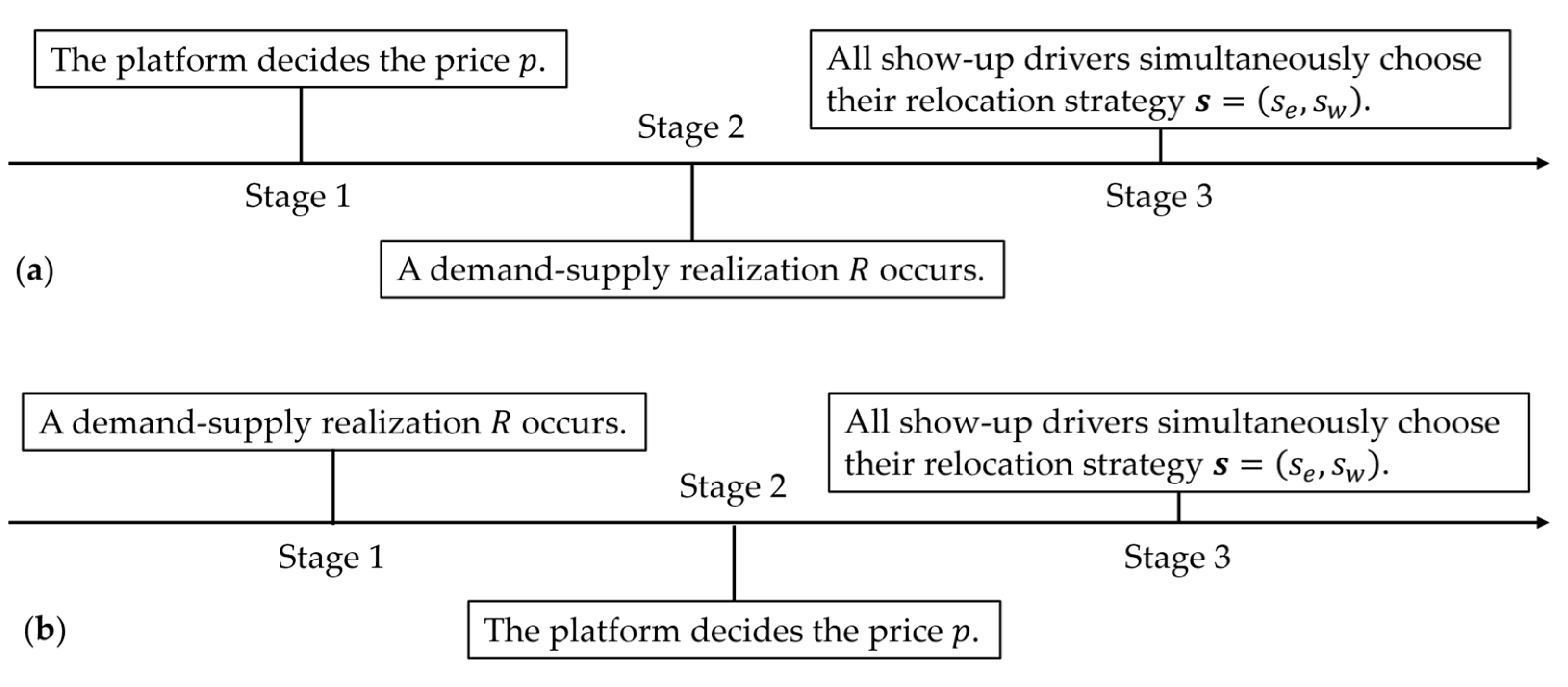
4.2. Platform’s Ex-Ante Pricing Strategy

In this subsection, we solve for the platform’s equilibrium ex-ante pricing strategy that maximizes its ex-ante expected profit. Substituting Equation (1) and the Nash equilibrium of the stage-3 subgame into Equations (8) and (9), we calculate the platform’s ex-ante expected profit as

$$\mathsf{\Pi }\left(p\right)={\sum }_R\mathrm{Pr}\left(R\right)\pi \left(p,\mathit{s}\left(p,R\right),R\right)=\left\{\begin{array}{cc}0& v_0\left(p,1\right)<0\\ 2rq\alpha p\min \left\{1-p,m\right\}& 0\le v_0\left(p,1\right)<c\\ \begin{array}{c}\left(2rq+2\left(1-r\right)r\left(1-q\right)q\right)\alpha p\min \left\{1-p,m\right\}\end{array}& v_0\left(p,2\right)<c\le v_0\left(p,1\right)\\ \begin{array}{c}\begin{array}{c}\begin{array}{c}\left(2r^{2}q+4\left(1-r\right)r\left(1-q\right)q\right)\alpha p\min \left\{1-p,m\right\}\\ +2\left(1-r\right)r{q}^2\alpha p\min \left\{1-p,2m\right\}\end{array}\end{array}\end{array}& v_0\left(p,2\right)\ge c\end{array}\right..$$

(11)

Solving the problem ${\mathrm{m}\mathrm{a}\mathrm{x}}_p\mathsf{\Pi }\left(p\right)$, we present the platform’s equilibrium ex-ante pricing strategy in Proposition 3, where ${\alpha }_1\left(m\right)=1-4m\left(c+c_0\right)$, ${\alpha }_2\left(m\right)=1-8m\left(c+2c_0\right)$, ${\alpha }_3\left(m\right)=1-\left(c+c_0\right)/\left(1-m\right)$, ${\alpha }_4\left(m\right)=1-2\left(c+2c_0\right)/\left(1-m\right)$, ${\alpha }_5\left(m\right)=1-2m\left(c+2c_0\right)/\left(\left(1/2+\mu m\right)\left(1/2-\mu m\right)\right)$, ${\alpha }_6\left(m\right)=1-\left(c+2c_0\right)/\left(1-2m\right)$ and $\mu ={\displaystyle \frac{r^2+2\left(1-r\right)r\left(1-q\right)}{2\left(1-r\right)rq}}$.

Proposition 3.

The platform’s equilibrium ex-ante prices ($p^{*}$) and induced show-up drivers’ relocation strategies are given in 

Table 2. The platform’s equilibrium prices and show-up drivers’ relocation strategies.

Conditions		${\mathit{p}}^{\mathit{*}}$	Realization	Show-Up Drivers’ Relocation Strategies
(i) $m\ge {\displaystyle \frac{1}{2}}$	(i-i) $\alpha \in \left({\alpha }_1\left(m\right),\overline{\alpha }\left(m\right)\right)$	${\displaystyle \frac{1}{2}}$	$R\in {\mathsf{\Omega }}_1\cup {\mathsf{\Omega }}_2\cup {\mathsf{\Omega }}_3$	$s_i=i$
	(i-ii) $\alpha \in \left({\alpha }_2\left(m\right),{\alpha }_1\left(m\right)\right]$	${\displaystyle \frac{1}{2}}$	$R\in {\mathsf{\Omega }}_1\cup {\mathsf{\Omega }}_3$	$s_i=i$
			$R\in {\mathsf{\Omega }}_2$	$s_i=j$($\ne i$)
	(i-iii) $\alpha \in \left[0,{\alpha }_2\left(m\right)\right]$	${\displaystyle \frac{1}{2}}$	$R\in {\mathsf{\Omega }}_1$	$s_i=i$
			$R\in {\mathsf{\Omega }}_2$	$s_i=j$($\ne i$)
			$R\in {\mathsf{\Omega }}_3$	$s_i=i$ if $R_{i,D}=1$ and $s_i=j$($\ne i$) if $R_{i,D}=0$
(ii) $m\in \left[{\displaystyle \frac{1}{2\left(\mu +1\right)}},{\displaystyle \frac{1}{2}}\right)$	(ii-i) $\alpha \in \left({\alpha }_3\left(m\right),\overline{\alpha }\left(m\right)\right)$	$1-m$	$R\in {\mathsf{\Omega }}_1\cup {\mathsf{\Omega }}_2\cup {\mathsf{\Omega }}_3$	$s_i=i$
	(ii-ii) $\alpha \in \left({\alpha }_4\left(m\right),{\alpha }_3\left(m\right)\right]$	$1-m$	$R\in {\mathsf{\Omega }}_1\cup {\mathsf{\Omega }}_3$	$s_i=i$
			$R\in {\mathsf{\Omega }}_2$	$s_i=j$($\ne i$)
	(ii-iii) $\alpha \in \left[0,{\alpha }_4\left(m\right)\right]$	$1-m$	$R\in {\mathsf{\Omega }}_1$	$s_i=i$
			$R\in {\mathsf{\Omega }}_2$	$s_i=j$($\ne i$)
			$R\in {\mathsf{\Omega }}_3$	$s_i=i$ if $R_{i,D}=1$ and $s_i=j$($\ne i$) if $R_{i,D}=0$
(iii) $m\in \left[{\displaystyle \frac{1}{2\left(\mu +2\right)}},{\displaystyle \frac{1}{2\left(\mu +1\right)}}\right)$	(iii-i) $\alpha \in \left({\alpha }_3\left(m\right),\overline{\alpha }\left(m\right)\right)$	$1-m$	$R\in {\mathsf{\Omega }}_1\cup {\mathsf{\Omega }}_2\cup {\mathsf{\Omega }}_3$	$s_i=i$
	(iii-ii) $\alpha \in \left({\alpha }_5\left(m\right),{\alpha }_3\left(m\right)\right]$	$1-m$	$R\in {\mathsf{\Omega }}_1\cup {\mathsf{\Omega }}_3$	$s_i=i$
			$R\in {\mathsf{\Omega }}_2$	$s_i=j$($\ne i$)
	(iii-iii) $\alpha \in \left[0,{\alpha }_5\left(m\right)\right]$	${\displaystyle \frac{1}{2}}+\mu m$	$R\in {\mathsf{\Omega }}_1$	$s_i=i$
			$R\in {\mathsf{\Omega }}_2$	$s_i=j$($\ne i$)
			$R\in {\mathsf{\Omega }}_3$	$s_i=i$ if $R_{i,D}=1$ and $s_i=j$($\ne i$) if $R_{i,D}=0$
(iv) $m\in \left(0,{\displaystyle \frac{1}{2\left(\mu +2\right)}}\right)$	(iv-i) $\alpha \in \left({\alpha }_3\left(m\right),\overline{\alpha }\left(m\right)\right)$	$1-m$	$R\in {\mathsf{\Omega }}_1\cup {\mathsf{\Omega }}_2\cup {\mathsf{\Omega }}_3$	$s_i=i$
	(iv-ii) $\alpha \in \left({\alpha }_6\left(m\right),{\alpha }_3\left(m\right)\right]$	$1-m$	$R\in {\mathsf{\Omega }}_1\cup {\mathsf{\Omega }}_3$	$s_i=i$
			$R\in {\mathsf{\Omega }}_2$	$s_i=j$($\ne i$)
	(iv-iii) $\alpha \in \left[0,{\alpha }_6\left(m\right)\right]$	$1-2m$	$R\in {\mathsf{\Omega }}_1$	$s_i=i$
			$R\in {\mathsf{\Omega }}_2$	$s_i=j$($\ne i$)
			$R\in {\mathsf{\Omega }}_3$	$s_i=i$ if $R_{i,D}=1$ and $s_i=j$($\ne i$) if $R_{i,D}=0$

.

The proof of Proposition 3 is shown in Appendix A.3.

Proposition 3 reveals that the commission rate does not have any impact on the platform’s equilibrium price if the supply size is large enough (Propositions 3(i) and 3(ii)). In this case, the platform has no incentive to decrease the ex-ante price to increase the demanded quantity in an area to accommodate two supplies, because such a large supply size makes one supply sufficient for the platform to maximize its ex-ante expected profit. However, a higher commission rate weakens show-up drivers’ incentive to relocate. Proposition 3(i) demonstrates that, once the commission rate increases to exceed the threshold $\alpha ={\alpha }_2\left(m\right)$, show-up drivers in an area without a realized demand no longer choose to relocate for $R\in {\mathsf{\Omega }}_3$. When it increases further to reach another threshold $\alpha ={\alpha }_1\left(m\right)$, show-up drivers choose not to relocate for $R\in {\mathsf{\Omega }}_2$. Proposition 3(ii) reveals a similar property, except that these two thresholds are replaced by $\alpha ={\alpha }_4\left(m\right)$ and $\alpha ={\alpha }_3\left(m\right)$, respectively.

In contrast, if the supply size is small enough (Propositions 3(iii) and 3(iv)), the commission rate affects both the platform’s ex-ante pricing strategy and show-up drivers’ relocation strategies. In this case, the platform needs to further consider whether to decrease the ex-ante price to induce two realized supplies to meet one realized demand for $R\in {\mathsf{\Omega }}_3$ because the supply size is so small. When the commission rate is high enough ($\mathsf{\alpha }>{\alpha }_5\left(m\right)$ in Propositions 3(iii) and $\mathsf{\alpha }>{\alpha }_6\left(m\right)$ in Propositions 3(iv)), it is not profitable for the platform to decrease the price to induce an additional realized supply to serve one realized demand as the commission collection (due to such a high commission rate) dominates the service quantity increase (due to a price decrease) in raising the platform’s ex-ante expected profit. When the commission rate is low enough, the commission collection is dominated by the service quantity increase, leading the platform to decrease the ex-ante price.

4.3. Platform’s Ex-Post Pricing Strategy

In this section, we solve for the platform’s ex-post pricing strategy that maximizes its ex-post expected profit for each of the demand–supply realizations. When substituting Equation (1) and the Nash equilibrium of the stage-3 subgame into Equation (9), we calculate the platform’s ex-post expected profit as follows:

For $R\in {\mathsf{\Omega }}_1\backslash \left(\begin{array}{cc}1& 1\\ 1& 1\end{array}\right)$,

$$\pi \left(p,\mathit{s}\left(p,R\right),R\right)=\left\{\begin{array}{cc}0& v_0\left(p,1\right)<0\\ \alpha p\min \left\{1-p,m\right\}& v_0\left(p,1\right)\ge 0\end{array}\right..$$

(12)

For $R=\left(\begin{array}{cc}1& 1\\ 1& 1\end{array}\right)$,

$$\pi \left(p,\mathit{s}\left(p,R\right),R\right)=\left\{\begin{array}{cc}0& v_0\left(p,1\right)<0\\ 2\alpha p\min \left\{1-p,m\right\}& v_0\left(p,1\right)\ge 0\end{array}\right..$$

(13)

For $R\in {\mathsf{\Omega }}_2$,

$$\pi \left(p,\mathit{s}\left(p,R\right),R\right)=\left\{\begin{array}{cc}0& v_0\left(p,1\right)<c\\ \alpha p\min \left\{1-p,m\right\}& v_0\left(p,1\right)\ge c\end{array}\right..$$

(14)

For $R\in {\mathsf{\Omega }}_3$,

$$\pi \left(p,\mathit{s}\left(p,R\right),R\right)=\left\{\begin{array}{cc}0& v_0\left(p,1\right)<0\\ \alpha p\min \left\{1-p,m\right\}& v_0\left(p,1\right)\ge 0 and v_0\left(p,2\right)<c\\ \alpha p\min \left\{1-p,2m\right\}& v_0\left(p,2\right)\ge c\end{array}\right..$$

(15)

With Equations (12)–(15), we solve the problem ${\mathrm{m}\mathrm{a}\mathrm{x}}_p\pi \left(p,\mathit{s}\left(p,R\right),R\right)$ for the platform’s equilibrium price for each of the demand–supply realizations and summarize the results in Proposition 4.

Proposition 4.

The platform’s equilibrium ex-post prices ($p^{**}\left(R\right)$) and induced show-up drivers’ relocation strategies are given in 

Table 3. The platform’s equilibrium ex-post prices and show-up drivers’ relocation strategies.

Conditions		Realization	${\mathit{p}}^{\mathit{*}\mathit{*}}\left(\mathit{R}\right)$	Show-Up Drivers’ Relocation Strategies
(i) $m\ge {\displaystyle \frac{1}{2}}$	(i-i) $\alpha \in \left({\alpha }_1\left(m\right),\overline{\alpha }\left(m\right)\right)$	$R\in {\mathsf{\Omega }}_1\cup {\mathsf{\Omega }}_2\cup {\mathsf{\Omega }}_3$	${\displaystyle \frac{1}{2}}$	$s_i=i$
	(i-ii) $\alpha \in \left({\alpha }_2\left(m\right),{\alpha }_1\left(m\right)\right]$	$R\in {\mathsf{\Omega }}_1\cup {\mathsf{\Omega }}_3$	${\displaystyle \frac{1}{2}}$	$s_i=i$
		$R\in {\mathsf{\Omega }}_2$	${\displaystyle \frac{1}{2}}$	$s_i=j$($\ne i$)
	(i-iii) $\alpha \in \left[0,{\alpha }_2\left(m\right)\right]$	$R\in {\mathsf{\Omega }}_1$	${\displaystyle \frac{1}{2}}$	$s_i=i$
		$R\in {\mathsf{\Omega }}_2$	${\displaystyle \frac{1}{2}}$	$s_i=j$($\ne i$)
		$R\in {\mathsf{\Omega }}_3$	${\displaystyle \frac{1}{2}}$	$s_i=i$ if $R_{i,D}=1$ and $s_i=j$($\ne i$) if $R_{i,D}=0$
(ii) $m\in \left[{\displaystyle \frac{1}{4}},{\displaystyle \frac{1}{2}}\right)$	(ii-i) $\alpha \in \left({\alpha }_3\left(m\right),\overline{\alpha }\left(m\right)\right)$	$R\in {\mathsf{\Omega }}_1\cup {\mathsf{\Omega }}_2\cup {\mathsf{\Omega }}_3$	$1-m$	$s_i=i$
	(ii-ii) $\alpha \in \left({\alpha }_2\left(m\right),{\alpha }_3\left(m\right)\right]$	$R\in {\mathsf{\Omega }}_1\cup {\mathsf{\Omega }}_3$	$1-m$	$s_i=i$
		$R\in {\mathsf{\Omega }}_2$	$1-m$	$s_i=j$($\ne i$)
	(ii-iii) $\alpha \in \left[0,{\alpha }_2\left(m\right)\right]$	$R\in {\mathsf{\Omega }}_1$	$1-m$	$s_i=i$
		$R\in {\mathsf{\Omega }}_2$	$1-m$	$s_i=j$($\ne i$)
		$R\in {\mathsf{\Omega }}_3$	${\displaystyle \frac{1}{2}}$	$s_i=i$ if $R_{i,D}=1$ and $s_i=j$($\ne i$) if $R_{i,D}=0$
(iii) $m\in \left(0,{\displaystyle \frac{1}{4}}\right)$	(iii-i) $\alpha \in \left({\alpha }_3\left(m\right),\overline{\alpha }\left(m\right)\right)$	$R\in {\mathsf{\Omega }}_1\cup {\mathsf{\Omega }}_2\cup {\mathsf{\Omega }}_3$	$1-m$	$s_i=i$
	(iii-ii) $\alpha \in \left({\alpha }_6\left(m\right),{\alpha }_3\left(m\right)\right]$	$R\in {\mathsf{\Omega }}_1\cup {\mathsf{\Omega }}_3$	$1-m$	$s_i=i$
		$R\in {\mathsf{\Omega }}_2$	$1-m$	$s_i=j$($\ne i$)
	(iii-iii) $\alpha \in \left[0,{\alpha }_6\left(m\right)\right]$	$R\in {\mathsf{\Omega }}_1\cup {\mathsf{\Omega }}_2$	$1-m$	$s_i=i$
		$R\in {\mathsf{\Omega }}_2$	$1-m$	$s_i=j$($\ne i$)
		$R\in {\mathsf{\Omega }}_3$	$1-2m$	$s_i=i$ if $R_{i,D}=1$ and $s_i=j$($\ne i$) if $R_{i,D}=0$

.

The proof of Proposition 4 is shown in Appendix A.4.

Proposition 4(i) shows that the platform’s ex-post pricing strategy is consistent with its ex-ante pricing strategy in Proposition 3(i), where a supply size in the highest interval ($m\ge 1/2$) leads the platform to choose an identical stationary price $p^{**}\left(R\right)=p^{*}=1/2$ regardless of whether the pricing strategy is decided ex-ante or ex-post. This is simply because such a high supply size makes it unnecessary for the platform to induce more than one realized supply to serve one realized demand. Naturally, show-up drivers’ relocation strategies are identical. More specifically, they choose not to relocate for all demand–supply realizations $R\in {\mathsf{\Omega }}_1\cup {\mathsf{\Omega }}_2\cup {\mathsf{\Omega }}_3$ when the commission rate is sufficiently high ($\alpha >{\alpha }_1\left(m\right)$). They choose not to relocate for $R\in {\mathsf{\Omega }}_1$ and to relocate for $R\in {\mathsf{\Omega }}_2\cup {\mathsf{\Omega }}_3$ when the commission rate is sufficiently low ($\alpha \le {\alpha }_1\left(m\right)$). Finally, they choose not to relocate for $R\in {\mathsf{\Omega }}_1\cup {\mathsf{\Omega }}_3$ and to relocate for $R\in {\mathsf{\Omega }}_2$ when the commission rate falls in the intermediate interval ($\mathsf{\alpha }\in \left({\alpha }_2\left(m\right),{\alpha }_1\left(m\right)\right]$).

However, a comparison of Propositions 4(ii) and 4(iii) with Propositions 3(ii)–3(iv) reveals how the supply size and the commission rate determine the difference between the ex-ante and ex-post pricing strategies. The difference can be shown schematically in Figure 1 for the case of $1/\left[2\left(\mu +1\right)\right]>1/4$ (the results are qualitatively unchanged when $1/\left[2\left(\mu +1\right)\right]\le 1/4$).

In Figure 2, Region ${\mathrm{I}}_1$ indicates that the platform chooses $p^{**}\left(R\right)=p^{*}=1/2$ and show-up drivers choose not to relocate for all $R\in {\mathsf{\Omega }}_1\cup {\mathsf{\Omega }}_2\cup {\mathsf{\Omega }}_3$. Region ${\mathrm{I}}_2$ indicates that the platform chooses $p^{**}\left(R\right)=p^{*}=1/2$ and show-up drivers choose not to relocate for $R\in {\mathsf{\Omega }}_1$ and to relocate for $R\in {\mathsf{\Omega }}_2\cup {\mathsf{\Omega }}_3$. Region ${\mathrm{I}}_3$ indicates that the platform chooses $p^{**}\left(R\right)=p^{*}=1/2$ and show-up drivers choose not to relocate for $R\in {\mathsf{\Omega }}_1\cup {\mathsf{\Omega }}_3$ and to relocate for $R\in {\mathsf{\Omega }}_2$. Therefore, Regions ${\mathrm{I}}_1$–${\mathrm{I}}_3$ together indicate that the platform’s ex-ante and ex-post pricing strategies are consistent and induce show-up drivers to choose identical relocation decisions for $m\ge 1/2$.

Region ${\mathrm{I}}_4$ indicates that the platform chooses an identical equilibrium $p^{**}\left(R\right)=p^{*}=1-m$ under both the ex-ante and ex-post pricing strategies and that show-up drivers choose not to relocate for all $R\in {\mathsf{\Omega }}_1\cup {\mathsf{\Omega }}_2\cup {\mathsf{\Omega }}_3$ in the equilibrium. Region ${\mathrm{I}}_5$ indicates that the platform also chooses an identical equilibrium $p^{**}\left(R\right)=p^{*}=1-m$ and show-up drivers choose not to relocate for $R\in {\mathsf{\Omega }}_1\cup {\mathsf{\Omega }}_3$ and to relocate for $R\in {\mathsf{\Omega }}_2$. Therefore, Regions ${\mathrm{I}}_4$–${\mathrm{I}}_5$ together also indicate that the platform’s ex-ante and ex-post pricing strategies are consistent and induce show-up drivers to choose identical relocation decisions for $m<1/2$. In summary, Regions ${\mathrm{I}}_1$–${\mathrm{I}}_5$ (the light grey regions in Figure 2) indicate the same relocation strategy of show-up drivers (they choose not to relocate themselves in Region ${\mathrm{I}}_4$ while they choose (not) to relocate themselves in Region ${\mathrm{I}}_5$ for $R\in {\mathsf{\Omega }}_2$ ($R\in {\mathsf{\Omega }}_1\cup {\mathsf{\Omega }}_3$)) under both the ex-ante and the ex-post pricing strategies even if the platform may choose different prices.

Region ${\mathrm{I}\mathrm{I}}_1$ reflects that the platform chooses the ex-ante pricing strategy with $p^{*}=1-m$ for all $R\in {\mathsf{\Omega }}_1\cup {\mathsf{\Omega }}_2\cup {\mathsf{\Omega }}_3$ and the ex-post strategy with $p^{**}\left(R\right)=1-m$ for $R\in {\mathsf{\Omega }}_1\cup {\mathsf{\Omega }}_2$ and $p^{**}\left(R\right)=1/2$ for $R\in {\mathsf{\Omega }}_3$. Accordingly, show-up drivers’ relocation decisions remain unchanged for $R\in {\mathsf{\Omega }}_1\cup {\mathsf{\Omega }}_2$—they choose not to relocate when $R\in {\mathsf{\Omega }}_1$ and to relocate when $R\in {\mathsf{\Omega }}_2$. However, when $R\in {\mathsf{\Omega }}_3$, the platform’s price change makes show-up drivers in an area without a realized demand who choose not to relocate under the ex-ante pricing strategy switch to relocating to the other area under the ex-post pricing strategy. Similarly, Region ${\mathrm{I}\mathrm{I}}_2$ also reflects that, only when $R\in {\mathsf{\Omega }}_3$, do the relocation decisions of show-up drivers in an area without a realized demand induced by the platform’s ex-post pricing strategy ($p^{**}\left(R\right)=1-2m$) become different from those induced by the platform’s ex-ante pricing strategy ($p^{*}=1-m$). Such show-up drivers who choose not to relocate under the ex-ante pricing strategy switch to relocating under the ex-post pricing strategy. In summary, Regions ${\mathrm{I}\mathrm{I}}_1$ and ${\mathrm{I}\mathrm{I}}_2$ (the dark grey regions) together reflect that, compared with the ex-ante pricing strategy, the platform’s ex-post pricing strategy decreases the price and induces more inter-area relocations of show-up drivers when $R\in {\mathsf{\Omega }}_3$, but it does not change the price and show-up drivers’ decisions when $R\in {\mathsf{\Omega }}_1\cup {\mathsf{\Omega }}_2$.

Regions ${\mathrm{I}\mathrm{I}\mathrm{I}}_1$–${\mathrm{I}\mathrm{I}\mathrm{I}}_4$ (the unfilled grey regions) capture the way in which show-up drivers’ relocation decisions are identical under the platform’s ex-ante and ex-post pricing strategies even if the prices under both pricing strategies can be different. As for show-up drivers’ relocation decisions, they choose not to relocate when $R\in {\mathsf{\Omega }}_1$ and to relocate for $R\in {\mathsf{\Omega }}_2\cup {\mathsf{\Omega }}_3$. As for the prices, Region ${\mathrm{I}\mathrm{I}\mathrm{I}}_1$ corresponds to the case where the platform’s ex-post pricing strategy sets an identical price $p^{**}\left(R\right)=p^{*}=1-m$ when $R\in {\mathsf{\Omega }}_1\cup {\mathsf{\Omega }}_2$ but decreases the price from $p^{*}=1-m$ to $p^{**}\left(R\right)=1/2$ when $R\in {\mathsf{\Omega }}_3$. Region ${\mathrm{I}\mathrm{I}\mathrm{I}}_2$ corresponds to the case where the platform’s ex-post pricing strategy increases the price from $p^{*}=1/2+\mu m$ to $p^{**}\left(R\right)=1-m$ when $R\in {\mathsf{\Omega }}_1\cup {\mathsf{\Omega }}_2$ but decreases the price from $p^{*}=1/2+\mu m$ to $p^{**}\left(R\right)=1/2$ when $R\in {\mathsf{\Omega }}_3$. Region ${\mathrm{I}\mathrm{I}\mathrm{I}}_3$ refers to the case where the platform’s ex-post pricing strategy increases the price from $p^{*}=1/2+\mu m$ to $p^{**}\left(R\right)=1-m$ when $R\in {\mathsf{\Omega }}_1\cup {\mathsf{\Omega }}_2$ but decreases the price from $p^{*}=1/2+\mu m$ to $p^{**}\left(R\right)=1-2m$ when $R\in {\mathsf{\Omega }}_3$. Region ${\mathrm{I}\mathrm{I}\mathrm{I}}_4$ refers to the case where the platform’s ex-post pricing strategy increases the price from $p^{*}=1-2m$ to $p^{**}\left(R\right)=1-m$ when $R\in {\mathsf{\Omega }}_1\cup {\mathsf{\Omega }}_2$ but sets an identical price $p^{**}\left(R\right)=p^{*}=1-2m$ when $R\in {\mathsf{\Omega }}_3$.

In summary, when $(m,\alpha )$ falls in Regions ${\mathrm{I}}_1$–${\mathrm{I}}_5$, either a sufficient supply size ($m\ge 1/2$) makes it unnecessary for the platform to use its (ex-ante or ex-post) pricing strategy to affect show-up drivers’ relocation strategies, or a high enough commission rate ($\alpha \ge \max \{{\alpha }_2\left(m\right),{\alpha }_6\left(m\right)\}$) gives show-up drivers sufficiently reduced motivation so as to relocate, which further restricts the platform’s flexibility to respond to demand–supply realizations. Thus, the platform chooses an identical ex-ante and ex-post price, leaving show-up drivers’ relocation decisions determined solely by a specific demand–supply realization. When $(m,\alpha )$ falls in Regions ${\mathrm{I}\mathrm{I}\mathrm{I}}_1–{\mathrm{I}\mathrm{I}\mathrm{I}}_4$, a low enough commission rate ($\alpha <\min \{{\alpha }_4\left(m\right),{\alpha }_5\left(m\right),{\alpha }_6\left(m\right)\}$) leads show-up drivers to have sufficiently high incentive to relocate. Thus, the platform can flexibly use the ex-post pricing strategy to respond to demand–supply realizations and maintain show-up drivers’ relocation decisions. Finally, when $(m,\alpha )$ falls in Regions ${\mathrm{I}\mathrm{I}}_1$ and ${\mathrm{I}\mathrm{I}}_2$, the commission rate is at an intermediate level. In this case, show-up drivers’ incentive to relocate is sensitive to the price. As a result, show-up drivers’ relocation decisions are accordingly changed (unchanged) whenever the price is changed (unchanged) by the ex-post pricing strategy.

5. Managerial Implications

5.1. The Impact of the Commission Rate Under the Ex-Ante Pricing Strategy

In this subsection, we analyze how the commission rate affects the platform’s profitability, drivers’ welfare, and pollutant emissions from an ex-ante perspective. We note again that both drivers’ welfare and pollutant emission are calculated from the relocation-cost-least equilibria given in Proposition 1. The results are summarized in Proposition 5.

Proposition 5.

Under the ex-ante pricing strategy, we have ${\displaystyle \frac{\partial \mathsf{\Pi }\left(p^{*}\right)}{\partial \alpha }}>0$, ${\displaystyle \frac{\partial V\left(p^{*}\right)}{\partial \alpha }}<0$ and ${\displaystyle \frac{\partial \mathsf{\Phi }\left(p^{*}\right)}{\partial \alpha }}=0$ except that 

(i) 

When $m\ge {\displaystyle \frac{1}{2}}$, $\mathsf{\Pi }\left(p^{*}\right)$ drops downwards at $\alpha ={\alpha }_1\left(m\right)$, and $V\left(p^{*}\right)$ jumps upwards at $\alpha ={\alpha }_2\left(m\right)$, and $\mathsf{\Phi }\left(p^{*}\right)$ drops downwards at both $\alpha ={\alpha }_1\left(m\right)$ and $\alpha ={\alpha }_2\left(m\right)$.

(ii) 

When $m\in \left[{\displaystyle \frac{1}{2\left(\mu +1\right)}},{\displaystyle \frac{1}{2}}\right)$, $\mathsf{\Pi }\left(p^{*}\right)$ drops downwards at $\alpha ={\alpha }_3\left(m\right), V\left(p^{*}\right)$ jumps upwards $\alpha ={\alpha }_4\left(m\right)$, and $\mathsf{\Phi }\left(p^{*}\right)$ drops downwards at $\alpha ={\alpha }_3\left(m\right)$ and $\alpha ={\alpha }_4\left(m\right)$.

(iii) 

When $m\in \left[{\displaystyle \frac{1}{2\left(\mu +2\right)}},{\displaystyle \frac{1}{2\left(\mu +1\right)}}\right)$, $\mathsf{\Pi }\left(p^{*}\right)$ and $\mathsf{\Phi }\left(p^{*}\right)$ drop downwards at $\alpha ={\alpha }_3\left(m\right)$ and $\alpha ={\alpha }_5\left(m\right)$, and $V\left(p^{*}\right)$ jumps upwards at $\alpha ={\alpha }_5\left(m\right)$.

(iv) 

When $m\in \left(0,{\displaystyle \frac{1}{2\left(\mu +2\right)}}\right)$, $\mathsf{\Pi }\left(p^{*}\right)$ and $\mathsf{\Phi }\left(p^{*}\right)$ drop downwards at $\alpha ={\alpha }_3\left(m\right)$ and $\alpha ={\alpha }_6\left(m\right)$, and $V\left(p^{*}\right)$ jumps upwards at $\alpha ={\alpha }_6\left(m\right)$.

The proof of Proposition 5 is shown in Appendix A.5.

Proposition 5 shows that an increase in the commission rate has discontinuous impacts on the platform’s expected profit, drivers’ expected relocation-cost-subtracted utility, and expected pollutant emission. This discontinuity is attributed to show-up drivers’ strategic inter-area relocations. For example, consider the jumps in Proposition 5(i). We know from Proposition 3(i), that show-up drivers in an area without a realized demand choose not to relocate in the case of $R\in {\mathsf{\Omega }}_3$ if the commission rate increases to reach a threshold $\alpha ={\alpha }_2\left(m\right)$. This leads to a saving of their relocation and congestion costs and a reduction of pollutant emission. However, it does not affect the platform’s profit because the supply size is so large ($m\ge 1/2$), meaning that one realized supply is enough to meet the demanded quantity in an area. If the commission rate increases further to reach another higher threshold $\alpha ={\alpha }_1\left(m\right)$, show-up drivers choose not to relocate in the case of $R\in {\mathsf{\Omega }}_2$. In this case, as $\alpha ={\alpha }_1\left(m\right)$ makes show-up drivers indifferent between relocating and not relocating, either decision leads to an identical expected relocation-cost-subtracted utility for drivers. However, their choice to not relocate make the platform lose profitable opportunities in the case of $R\in {\mathsf{\Omega }}_2$ but reduce pollutant emission. Other jumps in Proposition 5 can be understood in a similar manner except that the platform’s changes in the price at $\alpha ={\alpha }_4\left(m\right)$ for $m\in [1/\left[2\left(\mu +1\right)\right],1/2)$, $\alpha ={\alpha }_5\left(m\right)$ for $m\in [1/\left[2\left(\mu +2\right)\right],1/2(\mu +1\left)\right)$, and $\alpha ={\alpha }_6\left(m\right)$ for $m\in [0,1/\left[2\left(\mu +2\right)\right])$ have a negative impact on drivers’ expected relocation-cost-subtracted utility. However, this negative impact is dominated by the positive impact of the savings on relocation and congestion costs. Thus, drivers’ expected relocation-cost-subtracted utility jumps upwards at these threshold commission rates.

Proposition 5 also demonstrates that an increase in the commission rate has a positive impact on the platform’s expected profit, a negative impact on drivers’ expected relocation-cost-subtracted utility, and no impact on pollutant emission if the threshold commission rates in Proposition 5 are not reached. Together with its discontinuous impacts at these thresholds, we summarize that the impacts of an increase in the commission rate on the platform’s expected profit and drivers’ expected relocation-cost-subtracted utility are non-monotonic, while its impact on pollution emission is (weakly) negative. More importantly, this non-monotonic impact leads to two qualitatively different outcomes. On the one hand, an increase in the commission rate induces a win–loss outcome for the platform and drivers without any effect on the environment, as long as the commission rate does not reach the thresholds in Proposition 5. On the other hand, it results in a loss–win–win outcome for the platform, drivers, and the environment.

5.2. The Impact of the Commission Rate Under Ex-Post Pricing Strategy

In this subsection, we analyze how the commission rate affects the platform’s profitability, drivers’ welfare, and pollutant emission from an ex-ante perspective. The results are summarized in Proposition 6.

Proposition 6.

Under the ex-post pricing strategy, we have ${\displaystyle \frac{\partial \mathsf{\Pi }\left(p^{**}\left(R\right)\right)}{\partial \alpha }}>0$, ${\displaystyle \frac{\partial V\left(p^{**}\left(R\right)\right)}{\partial \alpha }}<0$ and ${\displaystyle \frac{\partial \mathsf{\Phi }\left(p^{**}\left(R\right)\right)}{\partial \alpha }}=0$, except that

(i) 

When $m\ge {\displaystyle \frac{1}{2}}$, $\mathsf{\Pi }\left(p^{**}\left(R\right)\right)$ drops downwards at $\alpha ={\alpha }_1\left(m\right)$, and $V\left(p^{**}\left(R\right)\right)$ jumps upwards at $\alpha ={\alpha }_2\left(m\right)$, and $\mathsf{\Phi }\left(p^{**}\left(R\right)\right)$ drops downwards at both $\alpha ={\alpha }_1\left(m\right)$ and $\alpha ={\alpha }_2\left(m\right)$.

(ii) 

When $m\in \left[{\displaystyle \frac{1}{4}},{\displaystyle \frac{1}{2}}\right)$, $\mathsf{\Pi }\left(p^{**}\left(R\right)\right)$ and $\mathsf{\Phi }\left(p^{**}\left(R\right)\right)$ drop downwards at $\alpha ={\alpha }_2\left(m\right)$ and $\alpha ={\alpha }_3\left(m\right)$, and $V\left(p^{**}\left(R\right)\right)$ jumps upwards at $\alpha ={\alpha }_2\left(m\right)$.

(iii) 

When $m\in \left(0,{\displaystyle \frac{1}{4}}\right)$, $\mathsf{\Pi }\left(p^{**}\left(R\right)\right)$ and $\mathsf{\Phi }\left(p^{**}\left(R\right)\right)$ drop downwards at $\alpha ={\alpha }_3\left(m\right)$ and $\alpha ={\alpha }_6\left(m\right)$, and $V\left(p^{**}\left(R\right)\right)$ jumps upwards at $\alpha ={\alpha }_6\left(m\right)$.

The proof of Proposition 6 is shown in Appendix A.6.

Proposition 6 shows that the impacts of an increase in the commission rate on the platform’s expected profit, drivers’ expected relocation-cost-subtracted utility, and expected pollutant emission under the ex-post pricing strategy are qualitatively the same as those under the ex-ante pricing strategy, except that some commission rate thresholds are different. This is numerically illustrated in Figure 3 in which the solid lines indicate the ex-ante pricing strategy while the dotted lines represent the ex-post pricing strategy. Therefore, both Propositions 5 and 6 highlight not only the non-monotonic impacts of the commission rate on the platform’s profitability, drivers’ welfare, and the environmental pollution, but also two qualitatively different outcomes. The practical implication of this result is that we need to identify the commission rate thresholds to distinguish the impact of a change in the commission rate (i.e., a win–loss outcome without an environmental effect or a loss–win–win outcome).

5.3. The Impact of Ex-Post Pricing Strategy

In this subsection, we use the results under the ex-ante pricing strategy as a benchmark and explore how the ex-post pricing strategy affects the platform’s profitability, drivers’ welfare, and pollutant emission from an ex-post perspective. The results are summarized in Proposition 7 where $\mathsf{\Delta }\mathsf{\Pi }=\mathsf{\Pi }\left(p^{**}\left(R\right)\right)-\mathsf{\Pi }\left(p^{*}\right)$, $\mathsf{\Delta }V=V\left(p^{**}\left(R\right)\right)-V\left(p^{*}\right)$ and $\mathsf{\Delta }\mathsf{\Phi }=\mathsf{\Phi }\left(p^{**}\left(R\right)\right)-\mathsf{\Phi }\left(p^{*}\right)$.

Proposition 7.

For any given $m$ and $\alpha \in \left[0,\overline{\alpha }\left(m\right)\right)$,

(i) 

When $\left(m,\alpha \right)$ falls in Regions ${\mathrm{I}}_1$–${\mathrm{I}}_5$, we have $\mathsf{\Delta }\mathsf{\Pi }=0$, $\mathsf{\Delta }V=0$, and $\mathsf{\Delta }\mathsf{\Phi }=0$.

(ii) 

When $\left(m,\alpha \right)$ falls in Regions ${\mathrm{I}\mathrm{I}}_1$ and ${\mathrm{I}\mathrm{I}}_2$, we have $\mathsf{\Delta }\mathsf{\Pi }\ge 0$, $\mathsf{\Delta }\mathsf{\Phi }\ge 0$, and $\mathsf{\Delta }V\ge (<)0$ for $c\le (>)c^{\#}$ where 

$$c^{\#}=\left\{\begin{array}{cc}\left(1-\alpha \right)\left[{\displaystyle \frac{1}{4m}}-\left(1-m\right)\right]-3c_0& m\ge {\displaystyle \frac{1}{4}}\\ \left(1-3m\right)\left(1-\alpha \right)-3c_0& m<{\displaystyle \frac{1}{4}}\end{array}\right..$$

(iii) 

When $\left(m,\alpha \right)$ falls in Regions ${\mathrm{I}\mathrm{I}\mathrm{I}}_1$–${\mathrm{I}\mathrm{I}\mathrm{I}}_4$, we have $\mathsf{\Delta }\mathsf{\Pi }>0$, $\mathsf{\Delta }V>0$, and $\mathsf{\Delta }\mathsf{\Phi }=0$.

The proof of Proposition 7 is shown in Appendix A.7.

Proposition 7(i) is intuitive. As the ex-post pricing strategy does not change the price and show-up drivers’ relocation decisions for all demand–supply realizations $R\in {\mathsf{\Omega }}_1\cup {\mathsf{\Omega }}_2\cup {\mathsf{\Omega }}_3$ in the case of a sufficiently large supply size, it naturally does not have any impact on the platform’s expected profit, drivers’ expected welfare, and expected pollutant emission. Proposition 7(iii) indicates that the ex-post pricing strategy benefits both the platform and drivers but has no impact on the environment. The reason for this result is that the ex-post pricing strategy does not change show-up drivers’ relocation decisions for all demand–supply realizations (and thus leads to an unchanged pollutant emission) but it allows the platform to respond with price choices to demand–supply realization more flexibly. Due to the fixed commission rate, both the platform and drivers benefit from this increased flexibility. Finally, Proposition 7(ii) reveals two qualitatively different insights: The ex-post pricing strategy makes both the platform and drivers better off at the cost of environmental pollution, or the platform solely benefits from it at the cost of both drivers and the environment. The relocation cost is a key factor to determine which outcome occurs. A sufficiently low (high) cost results in the former (latter) outcome.

In summary, Proposition 7 demonstrates that the platform has an incentive to switch from an ex-ante pricing strategy to an ex-post pricing strategy at the cost of pollutant emission, but that the impact of such a pricing strategy switch on drivers’ welfare depends on the relocation cost. This result establishes a possible relocation-cost cue to understand the debate among platforms, drivers, and regulators about how to balance the benefits of platforms, drivers, and the environment.

6. Discussion

In this section, we conduct a numerical case study with data in Didi Chuxing’s 2022 Annual Business and Social Responsibility Report [63] to roughly validate our model and its theoretical predictions in Section 6.1 and provide some actionable recommendations for ride-hailing platform managers and regulators in Section 6.2.

6.1. A Numerical Case Study

In this subsection, we use the data reported in Didi Chuxing’s 2022 Annual Business and Social Responsibility Report to show how a change in the commission rate would affect the platform’s profitability, drivers’ welfare, and pollutant emission. We estimate the (average) commission rates in 2021 and 2022 by

$${\alpha }_{2021}={\displaystyle \frac{{\mathrm{R}\mathrm{e}\mathrm{v}\mathrm{n}\mathrm{u}\mathrm{e}}_{2021}-{\mathrm{P}\mathrm{a}\mathrm{y}\mathrm{m}\mathrm{e}\mathrm{n}\mathrm{t}-\mathrm{t}\mathrm{o}-\mathrm{d}\mathrm{r}\mathrm{i}\mathrm{v}\mathrm{e}\mathrm{r}\mathrm{s}}_{2021}}{{\mathrm{R}\mathrm{e}\mathrm{v}\mathrm{n}\mathrm{u}\mathrm{e}}_{2021}}}\times 100\%={\displaystyle \frac{173.21-156.86}{173.21}}\approx 10\%$$

$${\alpha }_{2022}={\displaystyle \frac{{\mathrm{R}\mathrm{e}\mathrm{v}\mathrm{n}\mathrm{u}\mathrm{e}}_{2022}-{\mathrm{P}\mathrm{a}\mathrm{y}\mathrm{m}\mathrm{e}\mathrm{n}\mathrm{t}-\mathrm{t}\mathrm{o}-\mathrm{d}\mathrm{r}\mathrm{i}\mathrm{v}\mathrm{e}\mathrm{r}\mathrm{s}}_{2022}}{{\mathrm{R}\mathrm{e}\mathrm{v}\mathrm{n}\mathrm{u}\mathrm{e}}_{2022}}}\times 100\%={\displaystyle \frac{140.79-115.80}{140.79}}\approx 18\%$$

where the revenues and the payments to drivers are in the billions of RMB.

This indicates an 8% increase in Didi Chuxing’s commission rate in 2022 compared with that in 2021. Further, we use the numbers of annual active users and annual active drivers reported in the same file on the Didi Chuxing platform to estimate a normalized supply size as

$$m={\displaystyle \frac{\mathrm{T}\mathrm{h}\mathrm{e} \mathrm{n}\mathrm{u}\mathrm{m}\mathrm{b}\mathrm{e}\mathrm{r} \mathrm{o}\mathrm{f} \mathrm{a}\mathrm{n}\mathrm{n}\mathrm{u}\mathrm{a}\mathrm{l} \mathrm{a}\mathrm{c}\mathrm{t}\mathrm{i}\mathrm{v}\mathrm{e} \mathrm{d}\mathrm{r}\mathrm{i}\mathrm{v}\mathrm{e}\mathrm{r}\mathrm{s}}{\mathrm{T}\mathrm{h}\mathrm{e} \mathrm{n}\mathrm{u}\mathrm{m}\mathrm{b}\mathrm{e}\mathrm{r} \mathrm{o}\mathrm{f} \mathrm{a}\mathrm{n}\mathrm{n}\mathrm{u}\mathrm{a}\mathrm{l} \mathrm{a}\mathrm{c}\mathrm{t}\mathrm{i}\mathrm{v}\mathrm{e} \mathrm{u}\mathrm{s}\mathrm{e}\mathrm{r}\mathrm{s}}}={\displaystyle \frac{23}{587}}\approx 0.04$$

where the numbers of annual active users and annual active drivers are in the millions of people.

We finally fixed a very low congestion cost at $c_0=0.01$, riders’ show-up probability at $r=0.5$, and drivers’ show-up probability at $q=0.5$ to explore the impact of the 8% commission rate increase on the platform’s profitability, drivers’ welfare, and pollutant emission in three relocation-cost scenarios: $c=0.25$ (low), $c=0.5$ (intermediate), and $c=0.75$ (high). As we focus on the percent change in the platform’s profitability, drivers’ welfare, and pollutant emission, we fix the pollutant emission caused by a show-up driver’s relocation ($\epsilon$) at any positive level.

The numerical results under the ex-ante and the ex-post pricing strategies are summarized in

Table 4. The impact of the 8% commission rate increase under ex-ante pricing strategy.

The Relocation Cost	The Percent Change $\mathbf{in} \mathsf{\Pi }\left({\mathit{p}}^{\mathit{*}}\right)$	The Percent Change $\mathbf{in} \mathit{V}\left({\mathit{p}}^{\mathit{*}}\right)$	The Percent Change $\mathbf{in} \mathsf{\Phi }\left({\mathit{p}}^{\mathit{*}}\right)$
$c=0.25$	$+80.00\%$	$-10.06\%$	$0$
$c=0.5$	$+80.00\%$	$-11.36\%$	$0$
$c=0.75$	$+56.52\%$	$-7.44\%$	$-50.00\%$

and

Table 5. The impact of the 8% commission rate increase under ex-post pricing strategy.

The Relocation Cost	The Percent Change $\mathbf{in} \mathsf{\Pi }\left({\mathit{p}}^{\mathit{*}\mathit{*}}\left(\mathit{R}\right)\right)$	The Percent Change $\mathbf{in} \mathit{V}\left({\mathit{p}}^{\mathit{*}\mathit{*}}\left(\mathit{R}\right)\right)$	The Percent Change $\mathbf{in} \mathsf{\Phi }\left({\mathit{p}}^{\mathit{*}\mathit{*}}\left(\mathit{R}\right)\right)$
$c=0.25$	$+80.00\%$	$-10.03\%$	$0$
$c=0.5$	$+80.00\%$	$-11.27\%$	$0$
$c=0.75$	$+52.11\%$	$-11.21\%$	$-50.00\%$

, respectively. Table 4 and Table 5 demonstrate that, when the relocation cost is at the low ($c=0.25$) or the intermediate level ($c=0.5$), Didi Chuxing’s 8% increase in the commission rate does not change show-up drivers’ relocation strategies. It leads a win–loss outcome for the platform and the drivers, but has no impact on the environment. In contrast, when the relocation cost is high ($c=0.75$), this commission rate change triggers show-up drivers’ less-relocation decisions (${\alpha }_{2021}<{\alpha }_6\left(0.04\right)<{\alpha }_{2022}$), leading to a lower percent increase in the platform’s profitability, a lower percent decrease in drivers’ welfare, and a 50% decrease in pollutant emission. These numerical results coincide with the theoretical predictions in Propositions 5 and 6. In particular, the platform’s profitability increase given in Table 4 and Table 5 roughly and qualitatively reflects the decrease in the net loss (from 49.33 billion RMB to 23.78 billion RMB) reported in Didi Chuxing’s 2022 Annual Business and Social Responsibility Report.

6.2. Actionable Recommendations

Propositions 5–7 furnish the following actionable strategy recommendations for both ride-hailing platform managers and regulators.

Due to the concerns regarding drivers’ welfare and environmental impacts, ride-hailing platform managers are needed to increase drivers’ welfare and mitigate environmental harm via their pricing and commission strategies. If they fix at an ex-ante (ex-post) pricing strategy, Proposition 5 (6) highlights thresholds of the commission rate, ${\alpha }_2\left(m\right)$, ${\alpha }_4\left(m\right)$, ${\alpha }_5\left(m\right)$, and ${\alpha }_6\left(m\right)$ (${\alpha }_2\left(m\right)$ and ${\alpha }_6\left(m\right)$, at which a very small change in the commission rate discontinuously affects not only the surplus distribution between the platform and drivers, but also the pollutant emission. More specifically, the upward jump of drivers’ welfare and the downward jump of pollutant emission at those thresholds indicates that there exists a neighborhood of the commission rate around each of those thresholds, such that an increase in the commission rate within the neighborhood to improve drivers’ welfare and mitigate pollutant emission does not decrease the platform’s profitability too much. Thus, it is critical for platform managers to identify such commission rate thresholds based on the operating settings captured by parameters $c_0$, $c$, $m$, $r$, and $q$. With these identified thresholds, managers can figure out a best neighborhood of the commission rate that can meet the demanded improvement of drivers’ welfare and environment impacts. Finally, they can choose a commission rate within the neighborhood as a strategic response to improve drivers’ welfare and mitigate environmental impacts with a profitability loss as low as possible. If they want to fix their commission rates but change their pricing strategy from an ex-ante one to an ex-post one, Proposition 7(iii) underlines that this pricing strategy change can lead to a win–win outcome for both the platform and drivers without any negative impact on the environment when the commission rate and the supply size are small enough (Regions ${\mathrm{I}\mathrm{I}\mathrm{I}}_1$–${\mathrm{I}\mathrm{I}\mathrm{I}}_4$ in Figure 2). Otherwise, it either has no impact on the platform, drivers and the environment (Proposition 7(i)), or increases pollutant emission (Proposition 7(ii)).

From a regulatory perspective, if policymakers want to mitigate pollutant emission without any motivation to intervene in the strategic interactions among participants in the ride-hailing market, they can take measures to decrease the pollutant emission caused by a show-up driver’s relocation ($\epsilon$). This is because all of our results on the platform’s and show-up drivers’ behaviors in Propositions 1–7 are independent of $\epsilon$. Given that electric vehicles (EVs) produce far lower emissions than traditional fuel vehicles [64,65] and that ride-hailing platforms (such as Uber) still rely heavily on fuel vehicles in their fleets [66], a policy choice is to replace fuel vehicles by EVs or decrease the proportion of fuel vehicles in the ride-hailing fleets. This can be achieved by, for example, setting the lowest permitted proportion of EVs in platforms’ ride-hailing fleets [66,67] or levying a carbon tax on the emissions caused by platforms’ operations [68,69]. It is worth pointing out that once fuel vehicles are replaced by EVs or the proportion of fuel vehicles is decreased, the according investment is sunk. Thus, the strategic interactions between platforms and show-up drivers will be independent of such sunk investment.

7. Concluding Remarks

In this paper, we consider a city in which the realizations of ride-hailing demand and supply are spatially asynchronous and build two multiple-stage game-theoretical models to capture how a ride-hailing platform’s ex-ante and ex-post pricing strategies induce show-up drivers’ strategic inter-area relocations. We characterize the subgame perfect equilibria in which the platform’s ex-ante and ex-post pricing strategies and the follow-up equilibrium relocation strategies of show-up drivers are determined. Based on these equilibria, we obtain the following three main results.

(1) Given the platform’s commission rate, the (ex-ante or ex-post) pricing strategy, and the demand–supply realization, the Nash equilibria of the stage-3 subgame are not unique. Although drivers’ welfare and pollutant emission depend on specific inter-area relocations in equilibrium, the platform’s profit is not affected by the equilibrium multiplicity.

(2) The commission rate has non-monotonic discontinuous impacts on the platform’s profitability, drivers’ welfare, and pollutant emission under both pricing strategies. More specifically, when an increase in the commission rate does not change show-up drivers’ relocation strategies, it leads to a win–loss outcome for the platform and drivers, respectively, but the pollutant emission can be kept at a constant level. In contrast, when it changes show-up drivers’ relocation strategies, it leads to a loss–win–win outcome for the platform, drivers, and the environment, respectively. The result furnishes an important practical implication—that a change in the commission rate has two qualitatively different impacts on the platform’s profitability, drivers’ welfare, and pollutant emission (i.e., a win–loss outcome without environmental effect vs. a loss–win–win outcome). Thus, when evaluating the impact of an increased commission rate, we need to distinguish whether it changes show-up drivers’ relocation strategies to determine which outcome is induced.

(3) Relative to the ex-ante pricing strategy, the ex-post pricing strategy always benefits the platform at the cost of environmental pollution and enhances (reduces) drivers’ welfare when the relocation cost is low (high) enough. This result highlights that ride-hailing platforms have strong motivation to switch from an ex-ante pricing strategy to an ex-post pricing strategy and that this commercial profit-seeking motivation is intrinsically opposite to the interests of an environmental regulator. Moreover, in the case of a conflict between a platform and a regulator, whether drivers opt to support the platform or the regulator depends on the relocation cost—the platform (regulator) is supported when the relocation cost is low (high) enough. Therefore, the relocation cost can be viewed as a predictor of drivers’ opinions on whether to support the regulator’s banning the platform from using an ex-post pricing strategy (e.g., surge pricing).

We also roughly validate our model and its theoretical predictions with a numerical case study and provide some actionable strategies for platform managers and regulators.

Finally, we highlight some potential extensions of the current work. First, we make a cross-area homogeneity assumption and an intertemporal independence assumption of ride-hailing demand and supply to derive analytic results. From an engineering perspective, this assumption may be somewhat restrictive. Thus, it is worth introducing heterogeneous and intertemporally dependent demands and/or supplies to analyze the interaction between the platform and show-up drivers. Although this extension would make theoretical characterization difficult, managerial insights can be obtained by numerical analysis. Second, to theoretically characterize the implications of the platform’s ex-ante and ex-post pricing strategies on its profitability, drivers’ welfare, and pollutant emission, we assume a two-area city. Intuitively, this simplification assumption can be extended to capture a more general $n$-area city. However, the difficulty in characterizing the equilibrium relocation strategies of show-up drivers would hinder the exploration of clear analytic insights. Third, given the intrinsic inconsistency between a platform’s motivation and an environmental regulator’s interest, it is valuable to explicitly incorporate the regulations as a constraint in our model and examine how these regulations affect the interaction between the platform and show-up drivers and the corresponding outcomes for the platform’s profitability, drivers’ welfare, and pollutant emission. Fourth, our models and their implications are mainly theoretical. Although they are schematically validated by a numerical case study, more comprehensive and careful empirical work is needed to see to what degree or in what setting these theoretical implications are true and applicable in the real word.

References

1. Yan, C.; Zhu, H.; Korolko, N.; Woodard, D. Dynamic pricing and matching in ride-hailing platforms. Nav. Res. Logist. 2020, 67, 705–724. [Google Scholar] [CrossRef]
2. Feng, G.; Kong, G.; Wang, Z. We are on the way: Analysis of on-demand ride-hailing systems. M&SOM-Manuf. Serv. Oper. Manag. 2021, 23, 1237–1256. [Google Scholar]
3. Tirachini, A.; Del Río, M. Ride-hailing in Santiago de Chile: Users’ characterisation and effects on travel behaviour. Transp. Policy 2019, 82, 46–57. [Google Scholar] [CrossRef]
4. Tirachini, A. Ride-hailing, travel behaviour and sustainable mobility: An international review. Transportation 2020, 47, 2011–2047. [Google Scholar] [CrossRef]
5. Khaloei, M.; Ranjbari, A.; Laberteaux, K.; MacKenzie, D. Analyzing the effect of autonomous ridehailing on transit ridership: Competitor or desirable first-/last-mile connection? Transp. Res. Rec. 2021, 2675, 1154–1167. [Google Scholar] [CrossRef]
6. Ma, Y.; Chen, K.; Xiao, Y.; Fan, R. Does Online Ride-Hailing Service Improve the Efficiency of Taxi Market? Evidence from Shanghai. Sustainability 2022, 14, 8872. [Google Scholar] [CrossRef]
7. Brown, A.; LaValle, W. Hailing a change: Comparing taxi and ridehail service quality in Los Angeles. Transportation 2021, 48, 1007–1031. [Google Scholar] [CrossRef]
8. Meng, S.; Brown, A.; Barajas, J.M. Complements or competitors? Equity implications of taxis and ride-hail use in Chicago. J. Transp. Geogr. 2024, 120, 103973. [Google Scholar] [CrossRef]
9. Hall, J.V.; Krueger, A.B. An analysis of the labor market for Uber’s driver-partners in the United States. ILR Rev. 2018, 71, 705–732. [Google Scholar] [CrossRef]
10. Uber, Lyft Drivers Protest Across the US, Overseas|The Seattle Times. Available online: https://www.seattletimes.com/business/uber-lyft-drivers-plan-to-strike-in-cities-across-the-us/ (accessed on 10 March 2025).
11. Drivers Are Rising Up Against Uber’s ‘Opaque’ Pay System|WIRED. Available online: https://www.wired.com/story/drivers-are-rising-up-against-ubers-opaque-pay-system/ (accessed on 10 March 2025).
12. Lee, Y.; Chen, G.Y.H.; Circella, G.; Mokhtarian, P.L. Substitution or complementarity? A latent-class cluster analysis of ridehailing impacts on the use of other travel modes in three southern US cities. Transport. Res. Part D-Transport. Environ. 2022, 104, 103167. [Google Scholar] [CrossRef]
13. Ban, X.J.; Dessouky, M.; Pang, J.S.; Fan, R. A general equilibrium model for transportation systems with e-hailing services and flow congestion. Transp. Res. Pt. B-Methodol. 2019, 129, 273–304. [Google Scholar]
14. Giller, J.; Young, M.; Circella, G. Correlates of modal substitution and induced travel of Ridehailing in California. Transp. Res. Rec. 2024, 2678, 2046–2059. [Google Scholar] [CrossRef]
15. Qian, X.; Lei, T.; Xue, J.; Lei, Z.; Ukkusuri, S.V. Impact of transportation network companies on urban congestion: Evidence from large-scale trajectory data. Sust. Cities Soc. 2020, 55, 102053. [Google Scholar] [CrossRef]
16. Fageda, X. Measuring the impact of ride-hailing firms on urban congestion: The case of Uber in Europe. Pap. Reg. Sci. 2021, 100, 1230–1254. [Google Scholar] [CrossRef]
17. Li, Z.; Liang, C.; Hong, Y.; Zhang, Z. How do on-demand ridesharing services affect traffic congestion? The moderating role of urban compactness. Prod. Oper. Manag. 2022, 31, 239–258. [Google Scholar] [CrossRef]
18. Agarwal, S.; Mani, D.; Telang, R. The impact of ride-hailing services on congestion: Evidence from indian cities. M&SOM-Manuf. Serv. Oper. Manag. 2023, 25, 862–883. [Google Scholar]
19. Guda, H.; Subramanian, U. Your uber is arriving: Managing on-demand workers through surge pricing, forecast communication, and worker incentives. Manag. Sci. 2019, 65, 1995–2014. [Google Scholar] [CrossRef]
20. Afèche, P.; Liu, Z.; Maglaras, C. Ride-hailing networks with strategic drivers: The impact of platform control capabilities on performance. M&SOM-Manuf. Serv. Oper. Manag. 2023, 25, 1890–1908. [Google Scholar]
21. Feng, X.; Wang, M. Strategic driver’s acceptance-or-rejection behavior and cognitive hierarchy in on-demand platforms. Transp. Res. Pt. E-Logist. Transp. Rev. 2023, 176, 103175. [Google Scholar] [CrossRef]
22. Hu, X.; Zhou, S.; Luo, X.; Li, J.; Zhang, C. Optimal pricing strategy of an on-demand platform with cross-regional passengers. Omega-Int. J. Manag. Sci. 2024, 122, 102947. [Google Scholar] [CrossRef]
23. Zha, L.; Yin, Y.; Xu, Z. Geometric matching and spatial pricing in ride-sourcing markets. Transp. Res. Pt. C-Emerg. Technol. 2018, 92, 58–75. [Google Scholar] [CrossRef]
24. Sun, L.; Teunter, R.H.; Babai, M.Z.; Hua, G. Optimal pricing for ride-sourcing platforms. Eur. J. Oper. Res. 2019, 278, 783–795. [Google Scholar] [CrossRef]
25. Özkan, E. Joint pricing and matching in ride-sharing systems. Eur. J. Oper. Res. 2020, 287, 1149–1160. [Google Scholar] [CrossRef]
26. Besbes, O.; Castro, F.; Lobel, I. Surge pricing and its spatial supply response. Manag. Sci. 2021, 67, 1350–1367. [Google Scholar] [CrossRef]
27. Megantara, T.R.; Supian, S.; Chaerani, D. Strategies to Reduce Ride-Hailing Fuel Consumption Caused by Pick-Up Trips: A Mathematical Model under Uncertainty. Sustainability 2022, 14, 10648. [Google Scholar] [CrossRef]
28. Li, T.; Xu, M.; Sun, H.; Xiong, J.; Dou, X. Stochastic ridesharing equilibrium problem with compensation optimization. Transp. Res. Pt. E-Logist. Transp. Rev. 2023, 170, 102999. [Google Scholar] [CrossRef]
29. Xu, Y.; Ling, L.; Wu, J.; Xu, S. On-demand ride-hailing platforms under green mobility: Pricing strategies and government regulation. Transp. Res. Pt. E-Logist. Transp. Rev. 2024, 189, 103650. [Google Scholar] [CrossRef]
30. Taylor, T.A. On-demand service platforms. M&SOM-Manuf. Serv. Oper. Manag. 2018, 20, 704–720. [Google Scholar]
31. Bai, J.; So, K.C.; Tang, C.S.; Chen, X.; Wang, H. Coordinating supply and demand on an on-demand service platform with impatient customers. M&SOM-Manuf. Serv. Oper. Manag. 2019, 21, 556–570. [Google Scholar]
32. Wu, T.; Zhang, M.; Tian, X.; Wang, S.; Hua, G. Spatial differentiation and network externality in pricing mechanism of online car hailing platform. Int. J. Prod. Econ. 2020, 219, 275–283. [Google Scholar] [CrossRef]
33. Dong, Z.; Leng, M. Managing on-demand ridesharing operations: Optimal pricing decisions for a ridesharing platform. Int. J. Prod. Econ. 2021, 232, 107958. [Google Scholar] [CrossRef]
34. Zhong, Y.; Yang, T.; Cao, B.; Cheng, T.C.E. On-demand ride-hailing platforms in competition with the taxi industry: Pricing strategies and government supervision. Int. J. Prod. Econ. 2022, 243, 108301. [Google Scholar] [CrossRef]
35. Zhao, D.; Yuan, Z.; Chen, M.; Yang, S. Differential pricing strategies of ride-sharing platforms: Choosing customers or drivers? Int. Trans. Oper. Res. 2022, 29, 1089–1131. [Google Scholar] [CrossRef]
36. Li, J.; Huang, H.; Li, L.; Wu, J. Bilateral pricing of ride-hailing platforms considering cross-group network effect and congestion effect. J. Theor. Appl. Electron. Commer. Res. 2023, 18, 1721–1740. [Google Scholar] [CrossRef]
37. Zhao, C.L.; Sun, Y.; Wu, H.; Niu, D. Pricing model of ride-hailing platform considering rationally inattentive passengers. Transp. Lett. 2024, 1–11, in press. [Google Scholar] [CrossRef]
38. Chen, Q.; Lei, Y.; Jasin, S. Real-time spatial–intertemporal pricing and relocation in a ride-hailing network: Near-optimal policies and the value of dynamic pricing. Oper. Res. 2024, 72, 2097–2118. [Google Scholar] [CrossRef]
39. Bai, J.; Tang, C.S. Can two competing on-demand service platforms be profitable? Int. J. Prod. Econ. 2022, 250, 108672. [Google Scholar] [CrossRef]
40. Siddiq, A.; Taylor, T.A. Ride-hailing platforms: Competition and autonomous vehicles. M&SOM-Manuf. Serv. Oper. Manag. 2022, 24, 1511–1528. [Google Scholar]
41. Sun, Z.; Liu, J. Impacts of differentiated services and competition on the pricing strategies of ride-hailing platforms. Manag. Decis. Econ. 2023, 44, 3604–3624. [Google Scholar] [CrossRef]
42. Cachon, G.P.; Daniels, K.M.; Lobel, R. The role of surge pricing on a service platform with self-scheduling capacity. M&SOM-Manuf. Serv. Oper. Manag. 2017, 19, 368–384. [Google Scholar]
43. Chen, Y.; Hu, M. Pricing and matching with forward-looking buyers and sellers. M&SOM-Manuf. Serv. Oper. Manag. 2020, 22, 717–734. [Google Scholar]
44. Hu, B.; Hu, M.; Zhu, H. Surge pricing and two-sided temporal responses in ride hailing. M&SOM-Manuf. Serv. Oper. Manag. 2022, 24, 91–109. [Google Scholar]
45. Garg, N.; Nazerzadeh, H. Driver surge pricing. Manag. Sci. 2022, 68, 3219–3235. [Google Scholar] [CrossRef]
46. Tripathy, M.; Bai, J.; Heese, H.S. Driver collusion in ride-hailing platforms. Decis. Sci. 2023, 54, 434–446. [Google Scholar] [CrossRef]
47. Sui, Y.; Zhang, H.; Song, X.; Shao, F.; Yu, X.; Shibasaki, R.; Sun, R.; Yuan, M.; Wang, C.; Li, S.; et al. GPS data in urban online ride-hailing: A comparative analysis on fuel consumption and emissions. J. Clean Prod. 2019, 227, 495–505. [Google Scholar] [CrossRef]
48. Barnes, S.J.; Guo, Y.; Borgo, R. Sharing the air: Transient impacts of ride-hailing introduction on pollution in China. Transport. Res. Part D-Transport. Environ. 2020, 86, 102434. [Google Scholar] [CrossRef]
49. Naumov, S.; Keith, D. Optimizing the economic and environmental benefits of ride-hailing and pooling. Prod. Oper. Manag. 2023, 32, 904–929. [Google Scholar] [CrossRef]
50. Chen, J.; Li, W.; Zhang, H.; Cai, Z.; Sui, Y.; Long, Y.; Song, X.; Shibasaki, R. GPS data in urban online ride-hailing: A simulation method to evaluate impact of user scale on emission performance of system. J. Clean Prod. 2021, 287, 125567. [Google Scholar] [CrossRef]
51. Tikoudis, I.; Martinez, L.; Farrow, K.; Bouyssou, C.G.; Petrik, O.; Oueslati, W. Ridesharing services and urban transport CO2 emissions: Simulation-based evidence from 247 cities. Transport. Res. Part D-Transport. Environ. 2021, 97, 102923. [Google Scholar] [CrossRef]
52. Wang, X.; Wang, S.; Wang, L.; Fan, F. Has ridesourcing reduced haze? An analysis using the Didi app. Environ. Sci. Pollut. Res. 2021, 28, 45571–45585. [Google Scholar] [CrossRef]
53. Wang, Z.; Li, L.; Tang, J.; Xie, B.; Ge, J. Effect of ride sharing on air quality: Evidence from Shenzhen, China. J. Appl. Econ. 2022, 25, 197–219. [Google Scholar] [CrossRef]
54. Zhao, Y.; Wen, Y.; Wang, F.; Tu, W.; Zhang, S.; Wu, Y.; Hao, J. Feasibility, economic and carbon reduction benefits of ride-hailing vehicle electrification by coupling travel trajectory and charging infrastructure data. Appl. Energy 2023, 342, 121102. [Google Scholar] [CrossRef]
55. Gao, W.; Zhao, C.; Zeng, Y.; Tang, J. Exploring the Spatio-Temporally Heterogeneous Impact of Traffic Network Structure on Ride-Hailing Emissions Using Shenzhen, China, as a Case Study. Sustainability 2024, 16, 4539. [Google Scholar] [CrossRef]
56. Vives, X. Oligopoly Pricing; MIT Press: Cambridge, MA, USA, 1999. [Google Scholar]
57. Shin, H.; Tunca, T.I. Do firms invest in forecasting efficiently? The effect of competition on demand forecast investments and supply chain coordination. Oper. Res. 2010, 58, 1592–1610. [Google Scholar] [CrossRef]
58. Eslamipoor, R. Contractual Mechanisms for Coordinating a Sustainable Supply Chain with Carbon Emission Reduction. Bus. Strateg. Environ. 2025; in press. [Google Scholar] [CrossRef]
59. Cook, C.; Diamond, R.; Hall, J.V.; List, J.A.; Oyer, P. The gender earnings gap in the gig economy: Evidence from over a million rideshare drivers. Rev. Econ. Stud. 2021, 88, 2210–2238. [Google Scholar] [CrossRef]
60. Tracking Your Earnings|Driver App|Uber Ghana. Available online: https://www.uber.com/gh/en/drive/basics/tracking-your-earnings/ (accessed on 10 April 2025).
61. Bimpikis, K.; Candogan, O.; Saban, D. Spatial pricing in ride-sharing networks. Oper. Res. 2019, 67, 744–769. [Google Scholar] [CrossRef]
62. Tirole, J. The Theory of Industrial Organization; MIT Press: Cambridge, MA, USA, 1988. [Google Scholar]
63. DiDi Global-Financials-Corporate Report. Available online: https://ir.didiglobal.com/financials/annual-reports/default.aspx (accessed on 10 April 2025).
64. Jenn, A. Emissions benefits of electric vehicles in Uber and Lyft ride-hailing services. Nat. Energy 2020, 5, 520–525. [Google Scholar] [CrossRef]
65. Qiao, Q.; Zhao, F.; Liu, Z.; Hao, H.; He, X.; Przesmitzki, S.V.; Amer, A.A. Life cycle cost and GHG emission benefits of electric vehicles in China. Transport. Res. Part D-Transport. Environ. 2020, 86, 102418. [Google Scholar] [CrossRef]
66. Ku, Y.; Wu, P.; Ren, Q.; Wang, Y. The sequential pricing of ride-hailing system with rental service in the context of fleet electrification. J. Syst. Sci. Syst. Eng. 2024, 33, 77–105. [Google Scholar] [CrossRef]
67. Du, M.; Cheng, L.; Li, X.; Yang, J. Acceptance of electric ride-hailing under the new policy in Shenzhen, China: Influence factors from the driver’s perspective. Sust. Cities Soc. 2020, 61, 102307. [Google Scholar] [CrossRef]
68. Sepehriar, A.; Eslamipoor, R. An economical single-vendor single-buyer framework for carbon emission policies. J. Bus. Econ. 2024, 94, 927–945. [Google Scholar] [CrossRef]
69. Li, Y.; Li, X.; Jenn, A. Evaluating the emission benefits of shared autonomous electric vehicle fleets: A case study in California. Appl. Energy 2022, 323, 119638. [Google Scholar] [CrossRef]
Figure 1. The sequence of events. (a) Under the ex-ante pricing strategy. (b) Under the ex-post pricing strategy.
Sustainability 17 03896 g001
Figure 2. The comparison between Propositions 3 and 4.
Sustainability 17 03896 g002
Figure 3. A numerical illustration of the impact of the commission rate under ex-ante and ex-post pricing strategies ( r = q = 0.5 , c 0 = 0.2 , c = 0.2 , m = 0.1 and ε = 1 ).
Sustainability 17 03896 g003