Simulating Oil Spill Evolution and Environmental Impact with Specialized Software: A Case Study for the Black Sea

Abstract

Oil spills represent a significant environmental hazard, particularly in marine ecosystems, where their impacts extend to coastal infrastructure, biodiversity, and economic activities. This study utilizes GNOME v.47.2 (General NOAA Operational Modeling Environment) and ADIOS2 v.2.10.2 (Automated Data Inquiry for Oil Spills) to simulate and analyze oil spill dynamics in the Romanian sector of the Black Sea, focusing on trajectory prediction, hydrocarbon weathering, and shoreline contamination risk assessment. The research explores multiple spill scenarios involving different hydrocarbon types (light vs. heavy oils), vessel dynamics, and real-time environmental variables (wind, currents, temperature). The findings reveal that lighter hydrocarbons (e.g., gasoline, aviation fuel) tend to evaporate quickly, while heavier fractions (e.g., crude oil, fuel oil #6) persist in the marine environment and pose a higher risk of coastal pollution. In the first case study, a spill of 10,000 metric tons of medium oil (Arabian Medium EXXON) was simulated using GNOME v.47.2, showing that after 22 h, the slick reached the shoreline. Under forecasted hydro-meteorological conditions, 27% evaporated, 1% dispersed, and 72% remained for mechanical or chemical intervention. In the second simulation, 10,000 metric tons of gasoline were released, and within 6 h, 98% evaporated, with only minor residues reaching the shore. A real-world validation case was also conducted using the December 2024 Kerch Strait oil spill incident, where the model accurately predicted the early arrival of light fractions and delayed coastal contamination by fuel oil carried by subsurface currents. These results emphasize the need for future research focused on the vertical dispersion dynamics of heavier hydrocarbon fractions.

1. Introduction

Oil spills are major environmental hazards that can cause extensive damage to marine ecosystems, coastal economies, and human health. The severity of an oil spill depends on the type of hydrocarbon released, local oceanographic conditions, and the effectiveness of response measures. Computational modelling plays a crucial role in predicting spill behaviour and optimizing intervention strategies.

Major hydrocarbon spill incidents in the marine environment are predominantly associated with maritime transport and offshore operations. The study of such accidents is essential not only as a warning tool—illustrating the potential magnitude of these events—but also as critical documentation for emergency preparedness and response planning. To exemplify, several major marine pollution incidents involving accidental oil may be reminded. On 12 December 1999, the Erika, a Maltese-flagged tanker carrying 30,000 tons of oil, broke apart during a storm and sank in the Bay of Biscay, releasing approximately 20,000 tons of oil into the sea. The list of significant maritime accidents in the European region continues with the Haven oil tanker, which was loaded with over 144,000 tons of crude oil. In 1991, the vessel broke into three sections approximately 7 nautical miles off the coast of Genoa, France, resulting in a substantial spill. In 1993, the Braer oil tanker, carrying 85,000 tons of crude oil, ran aground on the Shetland Islands (Scotland), resulting in the complete loss of its cargo and severe contamination of the surrounding coastal waters. Another serious incident occurred in 1996 when the Sea Empress, transporting 130,824 tons of oil, ran aground on the coast of Wales, causing widespread coastal pollution. Additionally, offshore oil platform disasters have also raised serious concerns about marine environmental safety: the Ixtoc I blowout in 1979, the catastrophic Piper Alpha explosion in 1988, and the Deepwater Horizon incident in 2010. Each of these accidents resulted in massive hydrocarbon discharges into the marine environment, amounting to hundreds of thousands of tons, underscoring the vulnerability of marine ecosystems to both offshore and shipping-related oil pollution.

Oil spills pose significant environmental risks, necessitating advanced modelling techniques to predict their movement, transformation, and impact on marine ecosystems. Some of the most known comprehensive coupled oil spill prediction models include: The Oil Spill Contingency and Response model (OSCAR), The Spill Impact Model Application Package/Oil Modeling Application Package (SIMAP/OILMAP) The Blowout and Spill Occurrence Model (BLOSOM) and Three-dimensional Comprehensive Oil Spill Model for Surface and Underwater Spills (COMBOS3D) [1].

While OSCAR and BLOSOM are notable modeling tools in oil spill trajectory and fate simulation, they present specific limitations in the context of real-time, operational applications. OSCAR’s detailed simulations come at the cost of high computational demands and longer runtimes, which may not be practical in rapid response scenarios. BLOSOM offers advanced 3D hydrodynamic modeling but lacks native integration with NOAA observational data streams, thereby limiting its immediate applicability in coastal response operations. In contrast, GNOME v.47.2 and ADIOS2 v.2.10.2, developed and maintained by NOAA, are designed for operational use, allowing for swift data ingestion and scenario-based decision support in dynamic maritime environments.

There are also numerous studies that provide comparative analyses of the performance of the software tools employed [1,2,3,4,5], as well as research focusing on the effects of various dispersants potentially used in hydrocarbon pollution mitigation [6,7,8,9,10].

Several studies have explored the effectiveness of GNOME (General NOAA Operational Modelling Environment) and ADIOS2 (Automated Data Inquiry for Oil Spills) in simulating oil spill dynamics (National Oceanic and Atmospheric Administration, NOAA). These models provide crucial insights for oil spill response, helping authorities optimize mitigation strategies and assess environmental hazards.

1.1. GNOME for Oil Spill Trajectory Modelling

GNOME v.47.2 for Oil Spill Trajectory Modelling is widely recognized as an efficient tool for simulating oil spill drift and dispersion based on real-time environmental data such as wind, currents, and tides. It has been employed in various regional case studies to assess oil spill behaviour under different oceanographic conditions. Mahmood et al. (2024) conducted an oil spill trajectory simulation for the Buzzard Oilfield in the Outer Moray Firth, United Kingdom, using GNOME in combination with ADIOS2. Their study demonstrated that GNOME provides reliable predictions of oil drift, allowing emergency responders to anticipate shoreline impact zones and optimize containment strategies [11]. Similarly, NOAA’s operational models have been validated in numerous oil spill incidents, such as the Deepwater Horizon spill (2010), where GNOME was used to track the surface evolution of oil slicks and assess potential contamination risks to coastal infrastructure (NOAA, 2011) [12]. Studies suggest that GNOME’s accuracy improves when integrated with high-resolution oceanographic data, emphasizing the need for satellite and remote sensing assimilation [13].

1.2. ADIOS2 for Oil Weathering and Fate Simulation

ADIOS2 v.2.10.2 for Oil Weathering and Fate Simulation serves as a complementary tool to GNOME, focusing on oil weathering processes, including evaporation, emulsification, dispersion, and sedimentation. It provides critical data on oil type behaviour over time, which is essential for determining the most effective cleanup techniques. Research by Lame & Mahmood (2024) highlights how ADIOS2 enables an accurate assessment of oil spill fate, particularly for offshore crude oil spills [14]. Their study found that light hydrocarbons tend to evaporate quickly, whereas heavier crude oils persist in marine environments, necessitating mechanical recovery and bioremediation approaches [14]. Other research emphasizes the importance of combining GNOME v.47.2 and ADIOS2 v.2.10.2 to create more comprehensive spill response models. By integrating weathering data from ADIOS2 with GNOME’s hydrodynamic predictions, researchers can simulate oil transformation processes more effectively, leading to improved oil spill response planning [15].

2. Method

2.1. Research Objectives

The research aim is to simulate and analyze oil spill dynamics in the Romanian sector of the Black Sea, with a focus on spill trajectory prediction, hydrocarbon weathering, and shoreline contamination risk assessment, introducing the development of a rapid assessment and decision-support tool for managing hydrocarbon pollution incidents on board civilian ships or against offshore operational terminals and other critical infrastructure, due to mine hitting or other security threats in the region. Then, the primary aim is to enable onboard personnel to make optimal, time-sensitive decisions that may minimize environmental damage following a pollution event.

A representative scenario considered by the authors may be that of an explosion aboard an oil tanker carrying diverse cargoes in quantities of tens of thousands of tons. In such a case, a mine detonation can breach multiple cargo compartments, leading to the mixing of substances and the formation of new compounds with altered physicochemical properties compared to the original cargo. This not only complicates the environmental risk assessment but also escalates the urgency and complexity of operational decisions.

To maintain the vessel’s stability and prevent capsizing or sinking, the ship’s master may be forced to make critical choices, such as the controlled discharge of part of the cargo into the sea. The study, therefore, addresses key operational questions, including: which cargo type(s) should be prioritized for discharge, or in what quantity should the discharge occur to ensure minimal environmental impact? The answers to these questions depend on minimizing the likelihood of hydrocarbon pollutants reaching the shoreline and reducing the proportion of substances that remain undispersed, un-evaporated, or unburnt.

The proposed research method and tools integrates real-time satellite-based hydro-meteorological forecasting data with advanced pollution dispersion and management models (e.g., integrated pollution management software). A major emphasis is placed on the ultra-short decision-making timeframe required during such emergencies.

As case study limitation, it is important to note that this study does not delve into the long-term ecological consequences of hydrocarbon exposure on marine species or their role in mediating the spread of pollutants. Instead, the primary focus is resumed on the development of a practical, high-speed operational tool to support risk-informed decision-making process in severe pollution scenarios, involving hydrocarbon discharges from ships. To conduct the case studies in this research, two specialized software solutions were selected:

-

GNOME v.47.2 (General NOAA Operational Modelling Environment)—used to study the evolution of oil spills over time;

-

ADIOS2 v.2.10.2 (Automated Data Inquiry for Oil Spills)- used to assess intervention methods.

2.2. GNOME: Oil Spill Trajectory Modelling

GNOME v.47.2, developed by the National Oceanic and Atmospheric Administration (NOAA), is a powerful software designed for simulating the movement of hydrocarbon spills under various environmental conditions [12]. It models the dispersion, drift, and transformation of oil spills, accounting for influences such as wind, ocean currents, and tidal forces. GNOME v.47.2 offers several advanced simulation capabilities:

-

trajectory prediction—estimates the movement of oil spills under wind, ocean current, and meteorological conditions;

-

uncertainty analysis—assesses how trajectory predictions are affected by data inaccuracies in wind speed, currents, and pollutant properties;

-

hydrocarbon fate analysis—simulates the dispersion and evaporation of oil spills over time.

-

integration with ADIOS2—when used alongside ADIOS2 v.2.10.2, GNOME v.47.2 can track chemical and physical transformations of spilled oil, helping design intervention strategies.

GNOME v.47.2 operates by receiving input data about an oil spill scenario, then running simulations to predict oil slick evolution over time. The input parameters typically include type of spilled oil, meteorological and hydrological conditions (e.g., wind speed, currents) or geographical location of the spill. After inputting these parameters, GNOME generates trajectory models that show how the spill is likely to evolve under different conditions.

GNOME v.47.2 offers three operational modes:

• Standard Mode—uses predefined hydrodynamic and geographical data to simulate oil spill movement;
• GIS Mode—integrates with geographic information systems (GIS) for enhanced spatial visualization and mapping;
• Diagnostic Mode—allows real-time predictions and response planning, making it the most flexible option for emergency interventions.

In this paper, the Diagnostic Mode was used, because is particularly useful for real-time emergency response and predictive modelling. It includes: full access to model parameters and scaling options for greater customization, real-time hydrometeorological data integration, allowing accurate forecasting and adjustable uncertainty coefficients, using techniques such as Minimum Regret Estimation to minimize error in predictions. Regarding the hydrodynamic modelling approaches in GNOME, this software uses four different methods to simulate oil spill movement:

• Streamline Advection Model (SAC)—defines streamlines and their amplitudes, simulating how oil spreads within ocean currents;
• Wind-Driven Currents Model (WAC)—allows customization of wind amplitude and surface stress factors, modelling wind-induced drift at the ocean surface;
• Tidal Current Model (TAC)—simulates oil transport due to tidal forces. (Currently not applicable in all marine areas, being depended on the tidal influence);
• Diagnostic Circulation Model (DAC)—simulates current movements based on ocean surface height variations and dynamic flow conditions.

GNOME v.47.2 incorporates several physical and environmental parameters to enhance the accuracy of its predictions: depth-dependent friction coefficients (linear or nonlinear); advection and diffusion modelling; coriolis force adjustments; and atmosphere-ocean coupling coefficients. These advanced modelling capabilities make GNOME a highly effective tool for oil spill trajectory forecasting, ensuring proactive and informed response strategies.

A recent study by Zarochtunnisa et al. (2024) investigated GNOME’s application in detecting and modelling oil spills in the Madura Strait [16]. The study combined GNOME simulations with Sentinel Application Platform (SNAP v.11.0.0) software to analyse satellite images and map the spread of oil contamination. By integrating remote sensing data with GNOME, the researchers provided a more comprehensive understanding of oil spill behaviour, demonstrating the model’s ability to enhance oil spill monitoring and response strategies [16].

GNOME’s utility extends beyond spill trajectory prediction; it also plays a vital role in assessing the effectiveness of cleanup operations. The model has been employed to evaluate the impact of environmental conditions such as wind, currents, and tides on oil dispersion. This capability is essential for optimizing containment and recovery efforts, ensuring that response measures align with real-time environmental conditions. According to Zelenke et al. (2012), the software has been instrumental in real-time oil spill forecasting [17]. Additionally, research by Galt (1995) highlights GNOME’s accuracy in predicting oil slick movement under varying hydrodynamic conditions [18].

Furthermore, GNOME’s open-source nature and adaptability have made it an essential tool for researchers and policymakers in oil spill risk assessment. By integrating ocean circulation models and real-time observational data, GNOME v.47.2 enhances the accuracy of spill forecasts, ultimately supporting the development of more efficient oil spill response plans and mitigation policies.

Overall, GNOME v.47.2 has proven to be a valuable asset in oil spill tracking, risk assessment, and response planning. Its ability to integrate remote sensing data, simulate environmental interactions, and provide real-time spill movement predictions makes it an indispensable tool in modern environmental management and marine protection efforts. Future research should focus on improving model accuracy through enhanced data assimilation techniques and expanding GNOME’s applications to more complex spill scenarios, such as Arctic and deepwater environments.

2.2.1. Equations for Streamline Advection Modelling (SAC) [19]

a. Initial Point Equation

$${\displaystyle \frac{\partial \overrightarrow{V}}{\partial t}}+\left(𝛻\times \overrightarrow{V}\right)\times \overrightarrow{V}+𝛻\left({\displaystyle \frac{1}{2}}\overrightarrow{V}·\overrightarrow{V}\right)+f\times \overrightarrow{V}=-{\displaystyle \frac{1}{\rho }}𝛻P+{\displaystyle \frac{\partial }{\partial x}}\left(K_x{\displaystyle \frac{\partial \overrightarrow{V}}{\partial x}}\right)+{\displaystyle \frac{\partial }{\partial y}}\left(K_y{\displaystyle \frac{\partial \overrightarrow{V}}{\partial y}}\right)+{\displaystyle \frac{\partial }{\partial z}}\left(K_z{\displaystyle \frac{\partial \overrightarrow{V}}{\partial z}}\right)$$

(1)

b. Equation model for the transport current function

$$𝛻\left({\displaystyle \frac{1}{d}}𝛻\varphi \right)=0$$

(2)

c. The flow change equation

$${\displaystyle \frac{\partial h}{\partial t}}+𝛻·\left(h\overrightarrow{V}\right)+𝛻·\left(d\overrightarrow{V}\right)=0$$

(3)

d. Boundary conditions for Streamline Advection Modelling (SAC) [20]:

$${𝛻}^{2}A=0$$

(4)

-

all, without the flow limits, are current lines;

-

the difference between the values of the current lines in the channels give the transport;

-

natural flow limits do not prevent the flow;

-

the amplitude of the flow change is used to relax the non-divergent constraints and simulate a constant current wave.

2.2.2. Diagnostic Circulation Model (DAC) [21]

$${\displaystyle \frac{\partial \overrightarrow{V}}{\partial t}}+\left(𝛻\times \overrightarrow{V}\right)\times \overrightarrow{V}+𝛻\left({\displaystyle \frac{1}{2}}\overrightarrow{V}·\overrightarrow{V}\right)+f\times \overrightarrow{V}=-{\displaystyle \frac{1}{\rho }}𝛻P+{\displaystyle \frac{\partial }{\partial x}}\left(K_x{\displaystyle \frac{\partial \overrightarrow{V}}{\partial x}}\right)+{\displaystyle \frac{\partial }{\partial y}}\left(K_y{\displaystyle \frac{\partial \overrightarrow{V}}{\partial y}}\right)+{\displaystyle \frac{\partial }{\partial z}}\left(K_z{\displaystyle \frac{\partial \overrightarrow{V}}{\partial z}}\right)$$

(5)

$${\displaystyle \frac{\partial h}{\partial t}}+𝛻·\left(h\overrightarrow{V}\right)+𝛻·\left(d\overrightarrow{V}\right)=0$$

(6)

a. Surface elevation equation model

$$\epsilon {𝛻}^2\xi +J\left(d,\xi \right)=0$$

(7)

Boundary conditions for surface elevation equation model [22]:

-

the specified surface elevation along the isobar must have at least one open boundary within the model domain;

-

the correct boundary for surface elevation is to the right when facing shallow water if located in the Northern hemisphere;

-

shoreline boundaries can be ‘non-flowing’, elevated, or slightly inclined, depending on the simulated coastal current;

-

the natural boundary does not obstruct the flow.

2.2.3. Wind-Driven Current Modelling (WAC) [23]

$${\displaystyle \frac{\partial \overrightarrow{V}}{\partial t}}+\left(𝛻\times \overrightarrow{V}\right)\times \overrightarrow{V}+𝛻\left({\displaystyle \frac{1}{2}}\overrightarrow{V}·\overrightarrow{V}\right)+f\times \overrightarrow{V}=-{\displaystyle \frac{1}{\rho }}𝛻P+{\displaystyle \frac{\partial }{\partial x}}\left(K_x{\displaystyle \frac{\partial \overrightarrow{V}}{\partial x}}\right)+{\displaystyle \frac{\partial }{\partial y}}\left(K_y{\displaystyle \frac{\partial \overrightarrow{V}}{\partial y}}\right)+{\displaystyle \frac{\partial }{\partial z}}\left(K_z{\displaystyle \frac{\partial \overrightarrow{V}}{\partial z}}\right)$$

(8)

$${\displaystyle \frac{\partial h}{\partial t}}+𝛻·\left(h\overrightarrow{V}\right)+𝛻·\left(d\overrightarrow{V}\right)=0$$

(9)

Model equations for surface elevation

$$-fU=-g{\displaystyle \frac{\partial \xi }{\partial y}}+{\displaystyle \frac{{\tau }_y}{\rho \left(h+\xi \right)}}-{\displaystyle \frac{c{\left|U^2+V^2\right|}^{\frac{1}{2}}}{\left(h+\xi \right)}}V$$

(10)

$${\displaystyle \frac{\partial }{\partial x}}\left[\left(h+\xi \right)U\right]+{\displaystyle \frac{\partial }{\partial y}}\left[\left(h+\xi \right)V\right]=0$$

(11)

Boundary conditions for surface elevation [24]:

$$fV=-g{\displaystyle \frac{\partial \xi }{\partial x}}+{\displaystyle \frac{{\tau }_x}{\rho \left(h+\xi \right)}}-{\displaystyle \frac{c{\left|U^2+V^2\right|}^{\frac{1}{2}}}{\left(h+\xi \right)}}U$$

(12)

-

the wind speed can be specified across the entire domain, with at least one uplift point defined;

-

the uplift surface must be specified as high as the boundary points on one side and as low as the other;

-

the natural boundary does not obstruct the natural flow.

2.3. ADIOS2: Software for Oil Spill Response and Management

Effective oil spill prevention and response rely on specialized crisis management software that enables the estimation of the behaviour and evolution of spilled hydrocarbons. These tools assess the chemical and physical transformations of pollutants, their dispersion in marine environments, and their interaction with environmental parameters such as temperature, wind, ocean currents, wave characteristics, and atmospheric conditions. Beyond preventing marine pollution accidents, oil spill mitigation and cleanup strategies are critical to reducing environmental impact. The cleanup methods for oil spills in marine environments have evolved significantly over time, but oil spills continue to pose severe threats to marine ecosystems, leading to chemical exposure and toxicity to aquatic life. From this perspective, ADIOS2 (Automated Data Inquiry for Oil Spills) is a computational model designed to support oil spill response efforts. Developed by NOAA, ADIOS2 integrates a comprehensive database of over 1000 crude oil types and refined petroleum products, allowing for rapid estimations of oil behaviour once spilled into the marine environment. The software provides graphical and textual predictions, helping emergency response teams address key operational questions during spill response and cleanup efforts. ADIOS2 v.2.10.2 provides scientifically grounded predictions regarding the physical and chemical changes in spilled oil. Some of the core functions include:

-

viscosity evolution analysis—the software estimates changes in oil viscosity over time, helping answer critical questions regarding the effectively dispersion;

-

water content estimation in oil slicks—ADIOS2 predicts the rate at which oil absorbs water, assisting in planning the recovery process;

-

simulation of common oil spill cleanup techniques—ADIOS2 provides estimations on the effectiveness of standard response strategies, including: chemical dispersion (application of surfactants to break oil into small droplets), skimming (mechanical recovery of oil using skimmers), in-situ burning (controlled combustion of spilled oil), environmental weathering processes (including evaporation, sedimentation, and emulsification).

As limitation, while ADIOS2 v.2.10.2 currently provides such estimations, it does not explicitly model the use of herding agents-chemical surfactants applied to concentrate and thicken thin oil slicks to facilitate ISB or mechanical recovery. However, this technique has been recognized by NOAA and other agencies as a valuable pre-treatment, particularly in low-viscosity spills or remote response scenarios. Future extensions of ADIOS2 v.2.10.2 could benefit from the inclusion of herding agents as a discrete response mechanism within its decision-support outputs.

Additionally, ADIOS2 v.2.10.2 includes an extensive online help system and an electronic manual to assist users in utilizing its modelling capabilities. ADIOS2’s oil properties database provides detailed estimates of physical and chemical characteristics of crude oil and refined petroleum products. The software anticipates changes in oil properties post-spill using data compiled from multiple sources, including environmental agencies in Canada, the U.S. Department of Energy, and the petroleum industry. ADIOS2 v.2.10.2 incorporates scientific equations and computational algorithms to model the oil density variations over time, the viscosity changes and the rate of emulsification, the evaporation rates of oil on the water surface, the oil dispersion into the water column or the formation of oil-water emulsions and their persistence.

The mathematical framework is designed to use minimal input data, making it a practical tool for real-time oil spill response. The required hydrometeorological parameters include: wind speed, wave height, water temperature, salinity and density, type and quantity of spilled oil, and spill rate and duration. By combining oil weathering models with real-time environmental data, ADIOS2 v.2.10.2 may improve decision-making in oil spill emergency response, reducing ecological damage and enhancing cleanup efficiency.

Scientific computing has witnessed an exponential increase in data generation, necessitating efficient Input/Output (I/O) solutions to handle large-scale computations. ADIOS2 (Adaptable I/O System) has emerged as a key middleware in high-performance computing (HPC), enabling efficient data movement between memory, storage, and computational networks. Its ability to optimize parallel I/O, reduce bottlenecks, and integrate with advanced scientific simulations has led to widespread adoption in various domains.

One of the prominent applications of ADIOS2 v.2.10.2 in HPC is its role in accelerating large-scale data analysis. Cernuda et al. (2024) introduced Hades, a context-aware active storage framework that leverages ADIOS2 to manage weak scaling efficiently [25]. The study demonstrated how ADIOS2 improves performance in large-scale storage tiers, making it a crucial tool for high-performance computing environments. Similarly, Williams et al. (2024) explored ADIOS2’s integration with openPMD, specifically for Particle-in-Cell Monte Carlo simulations in plasma physics. Their findings highlighted ADIOS2’s ability to handle massive data flows with reduced I/O overhead, enhancing the efficiency of large-scale plasma simulations [26].

Beyond raw computational speed, ADIOS2 v.2.10.2 also plays a significant role in optimizing pre-computation strategies. Duwe and Kuhn (2024) developed DAI, a pre-computation framework that speeds up data analysis by improving read and write performance in ADIOS2-based applications [27]. Their work underscored how pre-computation techniques could drastically enhance data throughput, making ADIOS2 v.2.10.2 an even more powerful tool in real-world scientific applications. Similarly, Bhardwaj (2024) conducted a comparative study analysing the efficiency of ADIOS2 BP4, BP5, and HDF5 engines [8]. His research identified I/O bottlenecks in HPC workflows and highlighted ADIOS2’s superiority in handling parallel data processing compared to traditional HDF5-based methods.

In addition to its role in HPC and pre-computation, ADIOS2 v.2.10.2 has also been integrated into cloud computing and data management solutions. Song et al. (2024) introduced a region-aware self-describing data optimizer, specifically designed to enhance ADIOS2’s performance in distributed storage environments [28]. Their findings suggest that ADIOS2 can be effectively adapted for heterogeneous cloud architectures, ensuring scalable and high-performance data processing. ADIOS2 has been widely used in environmental impact studies and oil spill response planning.

Oil spill modelling plays a critical role in environmental protection, response planning, and mitigation strategies. Advanced computational tools such as ADIOS2 v.2.10.2 have been widely used to predict oil weathering, spreading, and degradation processes under different environmental conditions, being designed to simulate the behaviour of spilled oil by incorporating real-time meteorological and oceanographic data. Recent studies have demonstrated the efficiency of ADIOS2 v.2.10.2 in providing accurate predictions and enhancing response strategies for offshore and nearshore oil spills [28].

Efendi (2024) provided a comprehensive review of various oil spill cleanup methods, emphasizing the integration of ADIOS2 in oil weathering simulations [29]. The study highlighted ADIOS2’s ability to model continuous and batch oil spills in offshore environments, enabling responders to predict the dispersion, evaporation, and emulsification of oil over time. The research also compared ADIOS2 v.2.10.2 with other numerical models, concluding that its real-time simulation capabilities make it a valuable tool for decision-making in spill response planning [30].

Furthermore, ADIOS2’s application extends beyond standard response modelling to evaluating the effectiveness of oil spill cleanup technologies. The tool has been used to assess the impact of mechanical recovery, dispersant application, and in-situ burning under varying temperature, wind, and wave conditions. The ability of ADIOS2 to integrate with environmental datasets further enhances its utility, providing dynamic simulations that help in refining emergency response protocols and regulatory compliance [31].

Overall, the existing literature supports the significance of ADIOS2 in oil spill response and cleanup strategies. The model’s adaptability to real-time environmental conditions and its integration with other predictive tools position it as a cornerstone in modern oil spill response frameworks [32,33]. Further research is needed to enhance its predictive accuracy and expand its applications to more complex spill scenarios, including Arctic and deepwater environments.

2.4. The Methodology Applied for Real-Time Oil Spill Simulations

An important aspect of oil spill simulation is the incorporation of real-time meteorological conditions, wind data, and marine currents. Real-time data significantly enhances prediction accuracy, aiding in response planning and mitigation efforts for hydrocarbon spills. To integrate real-time weather and ocean current data, the General NOAA Operational Modelling Environment (GNOME v.47.2) was employed in its diagnostic mode [31,32]. This mode allows users to access a real-time global map, enabling precise positioning of the spill location and further, to retrieve hydrometeorological data from satellites specific to the selected area via the NOAA website (https://gnome.orr.noaa.gov, accessed on 30 November 2024 [34]).

For this study, the Black Sea region in the Romanian coast has been selected to analyse the possible risk occurring and crisis management scenarios development around the identified critical infrastructure, as depicted graphically in Figure 1. The major critical zones identified by the authors for which to apply a modelling case study are: point 1—the entrance in the Constanta Port and point 2—the oil terminal in Midia Port, with wider coverage for entire Romanian Economic Exclusive Zone.

Further, in order to define the model’s parameters, a customized map covering the Romanian coastal region and the identified key strategic points near Constanța was selected from the NOAA website. When utilizing GNOME v.47.2, it is recommended to choose a larger geographic area than the direct area of interest. This expanded selection allows for extended simulation times, such as 120-h oil spill evolution tracking. The initial selected map, displayed in Figure 2, will provide the initial basis for the simulation.

After selecting the respective map of studied area, in the subsequent stage, for the same selected domain, real-time wind and ocean current data are to be downloaded from the NOAA website (https://gnome.orr.noaa.gov/goods/currents/HYCOM/get_data, accessed on 30 November 2024). These datasets, which will facilitate the realistic simulations in the Black Sea region, have been saved locally and subsequently have been imported into GNOME software for modelling and simulation [3].

The process of acquiring marine current data is illustrated in Figure 3, which also applies in case of wind data retrieval. In this representation has been reflected the input of the selected map coordinates in second phase of modelling, to obtain marine currents data (similarly, for wind data) from the GNOME website. Consequently, based on the geospatial selection performed in the previous step, real-time wind and marine currents data have been retrieved by inputting the same geographic coordinates as those used for the map selection process illustrated above in Figure 2.

By entering the same geographic coordinates as in the map selection step (see Figure 2), the model developers will ensure that the real-time wind and marine currents datasets will be fully aligned with the defined simulation area. Following the initial phase of model construction, the detailed steps for generating real-time maps and environmental data for GNOME v.47.2 simulations are outlined below, applied in practice for the present case study by the authors:

✓

access NOAA’s GNOME on website link: http://gnome.orr.noaa.gov/goods, accessed on 30 November 2024;

✓

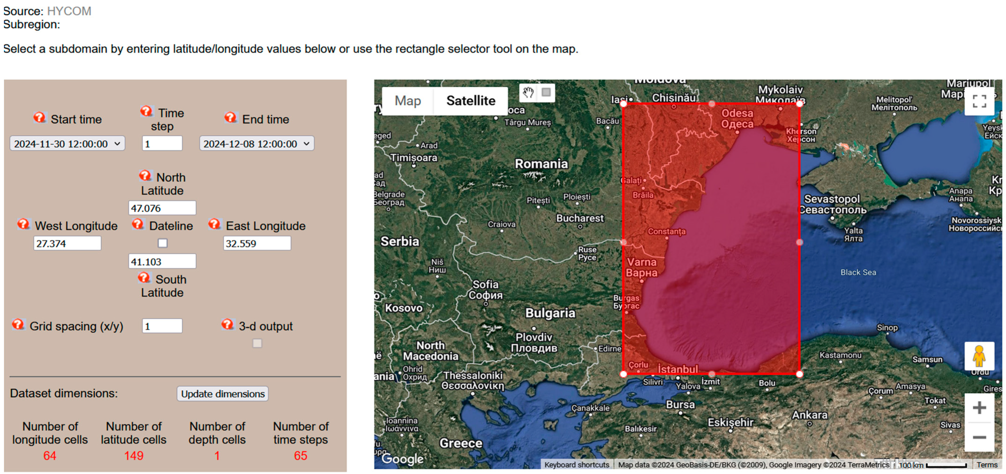
select “Global Custom Map Generator” to define a region of interest considered in the study;

✓

click “Draw Rectangle” to specify the geographic area (as shown in Figure 2);

✓

click “Get Map”, and save the generated coast.bna file, which will later be used in GNOME for map insertion;

✓

load the coast.bna file into GNOME v.47.2 software;

✓

navigate to ‘Maps > Load’, then import the file to generate a customized simulation map;

✓

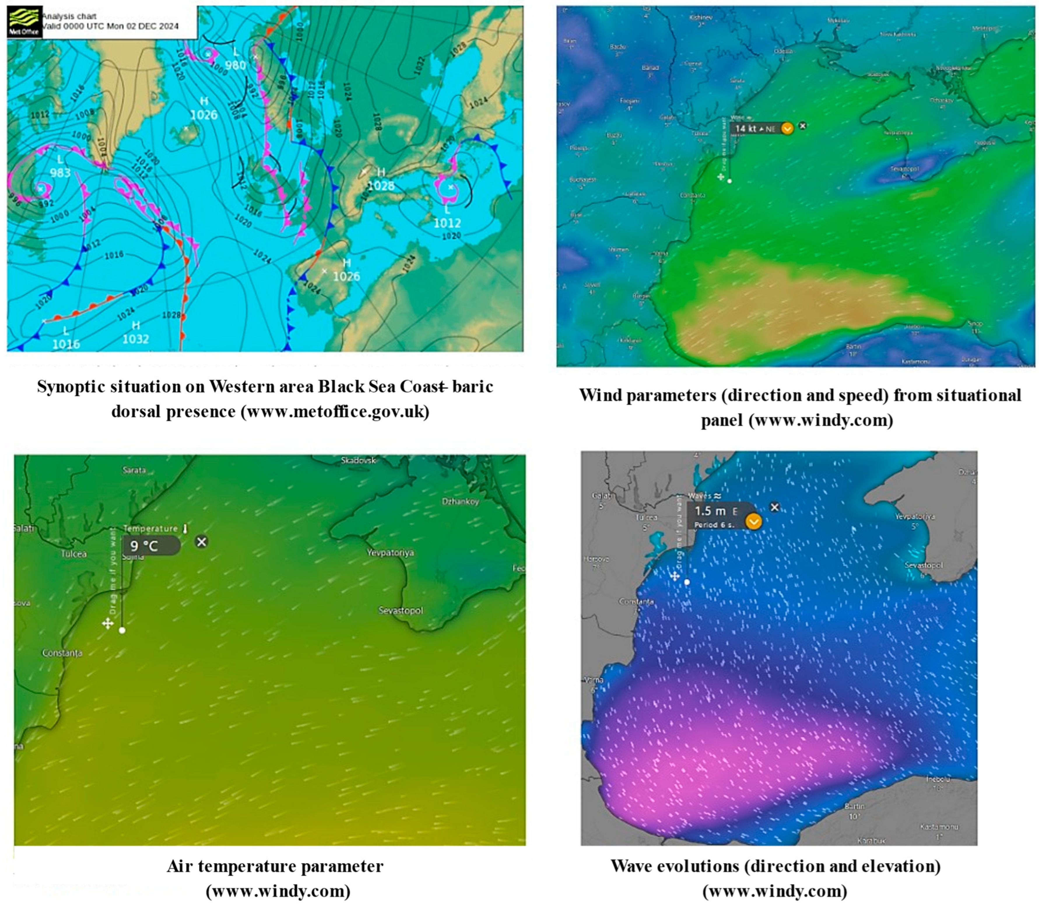
retrieve real-time wind and ocean current data;

✓

download separate datasets for wind and current conditions from NOAA (http://gnome.orr.noaa.gov/goods, accessed on 30 November 2024);

✓

in case of marine/ocean currents, refer to Figure 3;

✓

load these datasets into GNOME v.47.2 under the “Movers” category;

✓

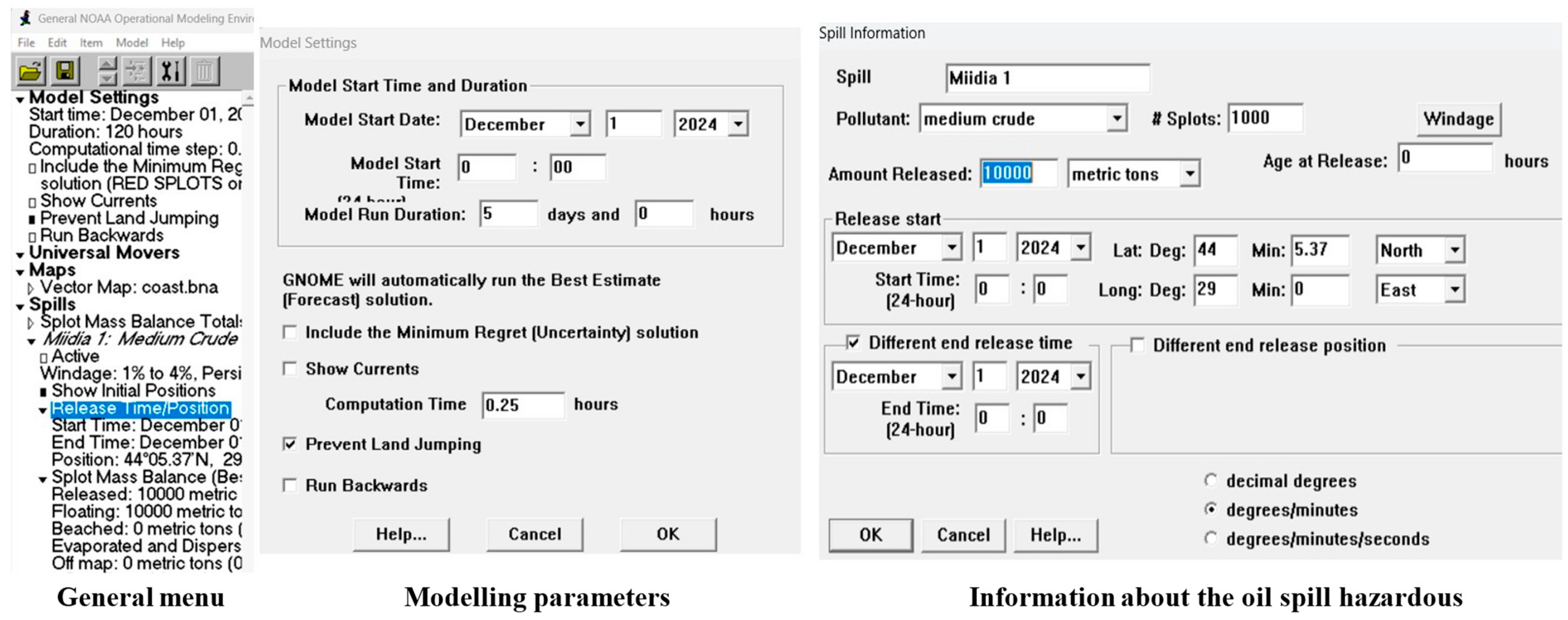
executing Oil Spill Simulations in GNOME v.47.2.

Once the initial conditions and environmental data were successfully integrated into GNOME, simulations were conducted to track the evolution of oil slicks in real-time using GNOME’s Diagnostic Mode.

Detailing the study hypothesis approached in practice by the authors for present model development, the initial simulation time was set to 1 December 2024, at 00:00, with a 120-h duration of simulation process, the selected geographic region supporting such extended simulations. However, if the simulation fails to progress through the applied time interval, longer or shorter, one potential solution will be to increase the selected map area to provide a broader spatial context.

The 120-h simulation window was chosen based on NOAA’s operational standards for short- to medium-range forecasting of coastal marine spills [12]. This window provides sufficient time to capture the evolution of spill trajectories while limiting the accumulation of model uncertainty. Then, to examine seasonal effects, the authors have conducted simulations using winter and summer ocean current datasets, sourced from NOAA data. Results revealed that seasonal variations in currents significantly influenced spill trajectories. Under winter conditions, the spill spread radius reached approximately 48 km after 120 h, compared to 35 km in summer. These differences are primarily due to stronger, more directional currents during winter months, which accelerate and extend offshore transport.

Following the setup of initial conditions, oil slicks (including crude oil, gasoline, and other hydrocarbons) were introduced at predefined strategic points offshore, at various distances from the coastline. The simulations monitored the trajectory, dispersion, and shoreline impact of the oil spill over time, the authors being focused during the simulation on the location where oil slicks reached the shore, the time elapsed before shoreline impact, and whether the spill affected key strategic locations along the Romanian coastline. By integrating GNOME with real-time wind and current data, this study aims to demonstrate a systematic approach to modelling oil spills in the Black Sea. The ability to dynamically adjust map coverage and simulation duration may make GNOME an effective tool for oil spill response planning.

During the simulation, three key output metrics were systematically monitored to evaluate the effectiveness of the response model:

-

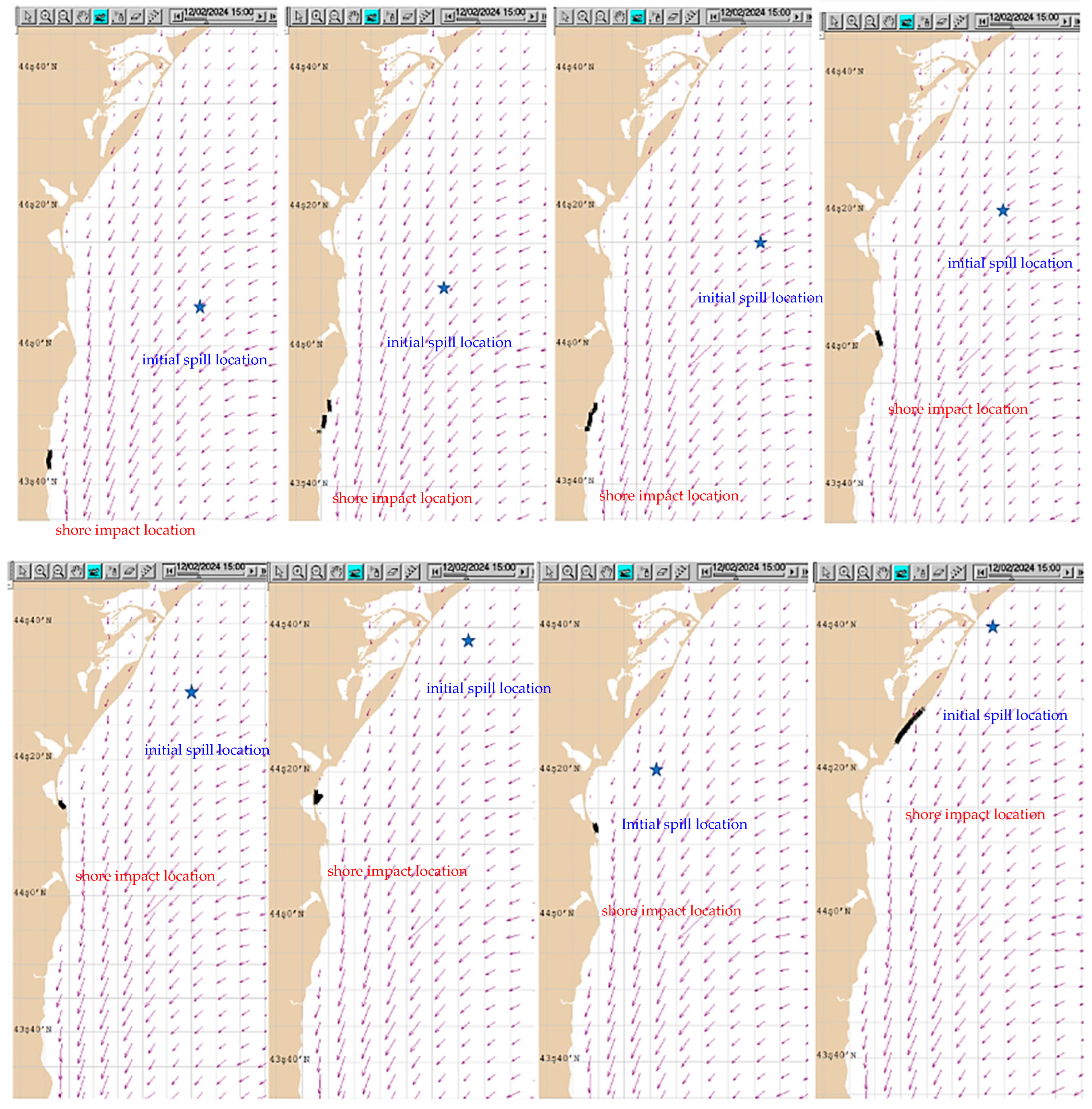
shoreline impact location—the exact geographical coordinates and zones where the oil slick first made landfall;

-

time to shoreline contact—the duration, in hours, from the initial spill to the first contact with the coast;

-

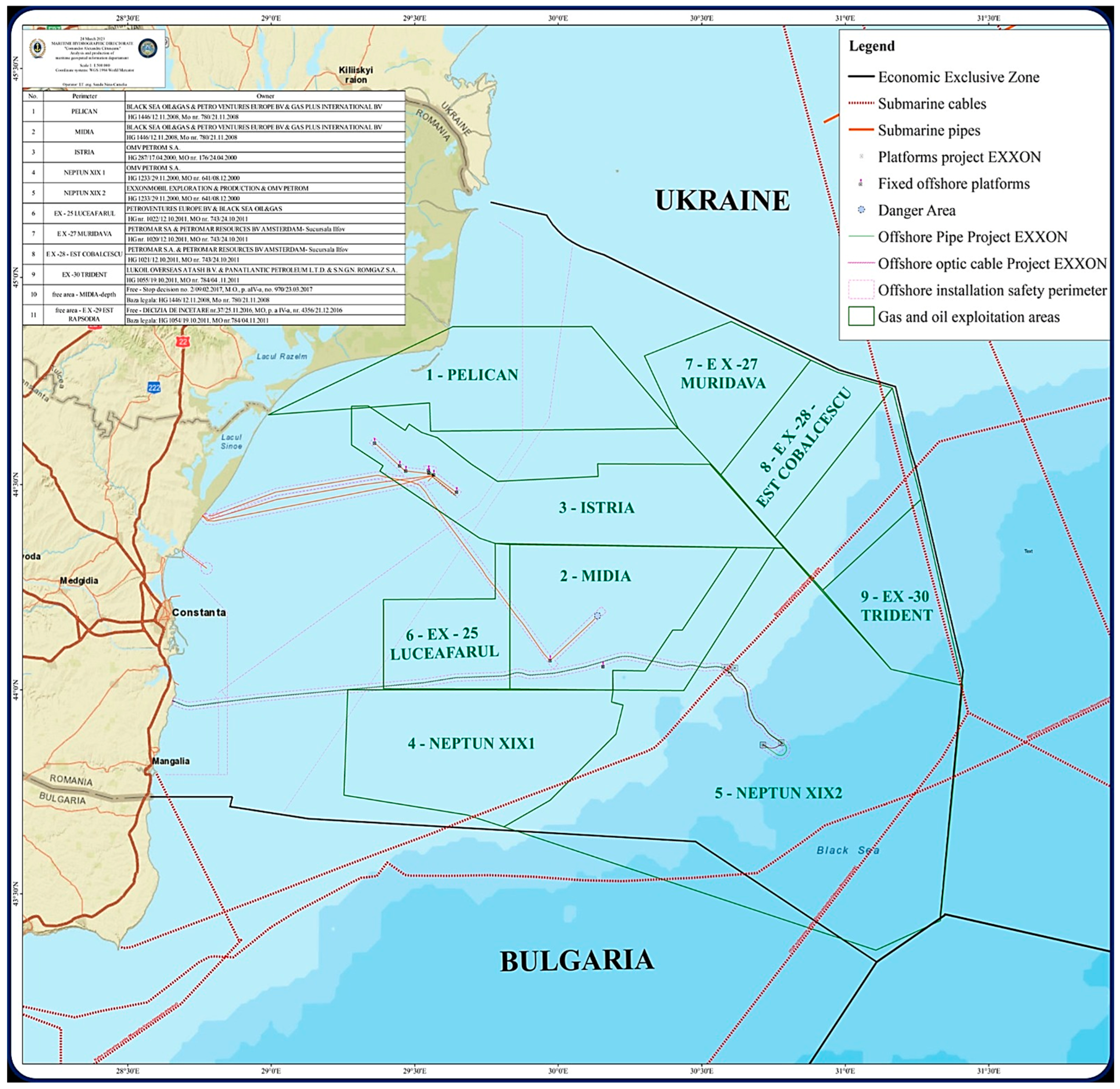
proximity to critical infrastructure—whether the oil slick trajectory intersected with high-risk strategic locations, such as port facilities (e.g., Constanța, Midia), pipelines, or ecological protection zones.

The meteorological context at the time of the oil spill discharging, is described by the synoptic hydro-meteorology situation, encompassing the wind, temperature and the waves, that is taken from the specialized websites (available online at: www.windy.com, and https://www.metoffice.gov.uk/weather/maps-and-charts/surface-pressure, accessed on 1 December 2024), being graphically depicted in Figure 4. This weather context is also important to consider when initiating spill response procedures, when for example, too high waves can make it difficult or may hamper the intervention at sea.

In the first simulation scenario (see Figure 6), involving a 10,000-metric-ton spill of Arabian Medium oil, the GNOME model predicted that the slick would reach the shoreline after 22 h. The impacted zone was located adjacent to the coastal region of Constanța, confirming the risk to essential infrastructure. This spatial and temporal information was visualized in the simulation output and supported by real-time hydro-meteorological inputs. To complement the trajectory data, the authors have further analyzed the evolution of pollutant fractions (evaporated, dispersed, mechanically recovered, and residual), offering in the next sections a tabular breakdown of the slick’s temporal behavior, illustrating how GNOME v.47.2 and ADIOS2 v.2.10.2 can provide a reliable, time-sensitive framework for evaluating shoreline impact and supporting targeted response actions.

3. Model Simulation in GNOME and ADIOS2 Software: Results Interpretation

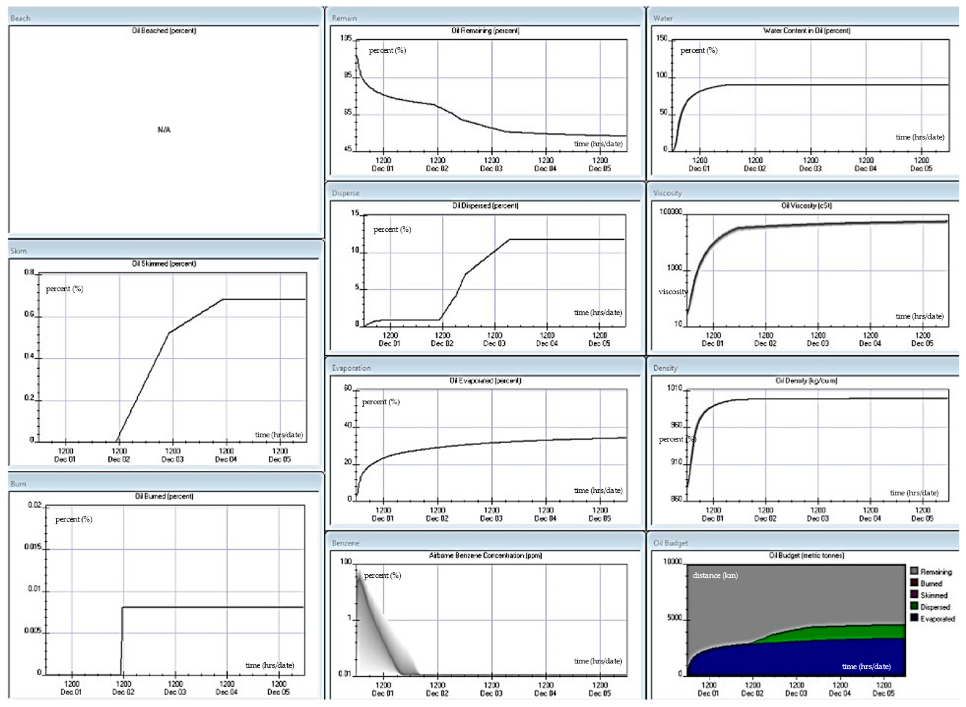
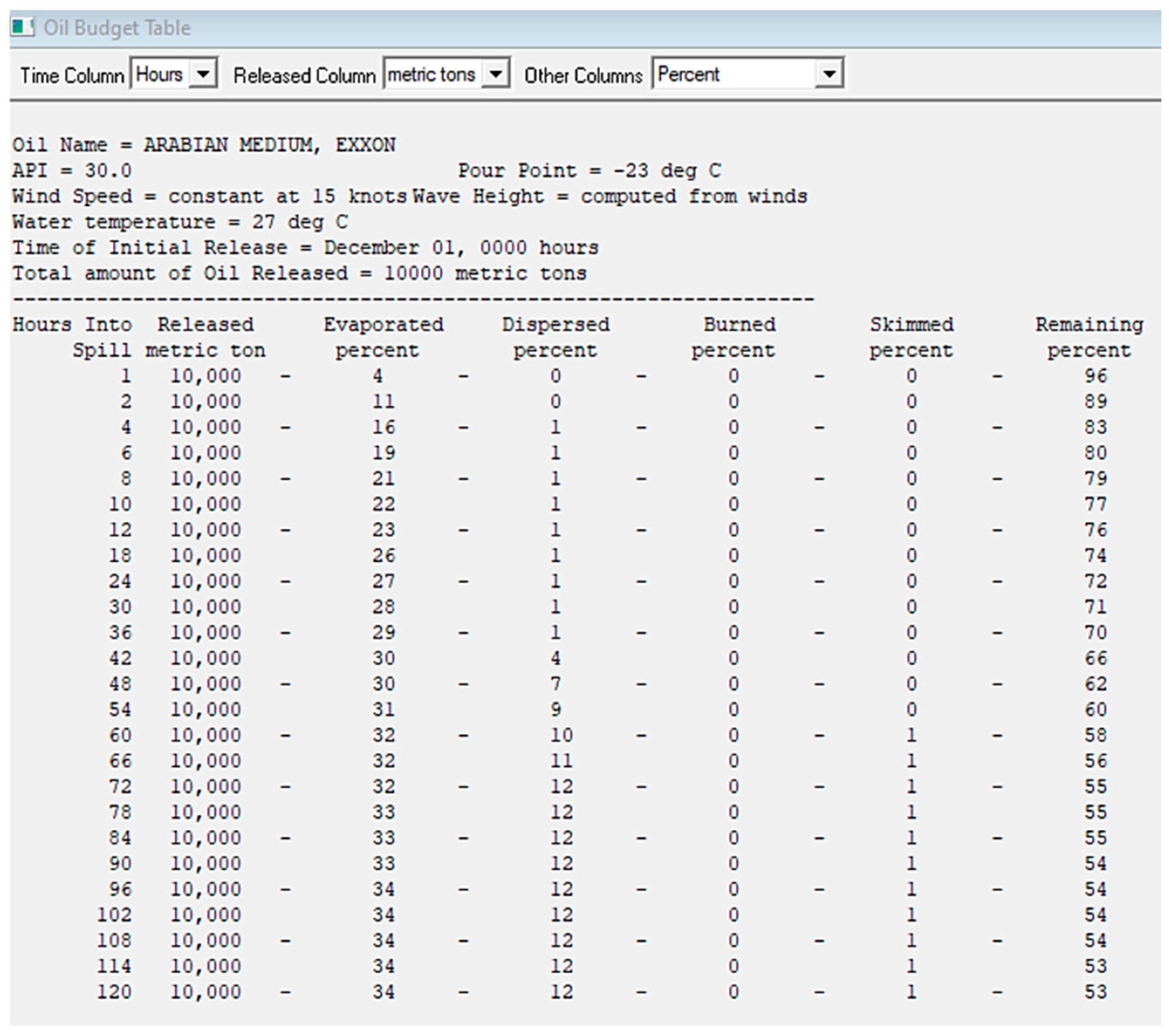
3.1. Scenario Analysis for Medium Crude Oil Spill—Static Simulation

For a first case study the authors have considered a spill of 10,000 metric tons of medium oil, simulated as occurred at the following coordinates on the map: latitude: 44 degrees and 5.37 min North; longitude: 29 degrees and 0 min East. All the discharge is happening at the same point on the map and at a well-defined time—this case is emulating a hazardous accident that suddenly discharges the entire amount at a certain location, and it can occur for example when an oil tanker has a structural (catastrophic) accident, it can no longer advance and quickly discharges the oil in the location where it is stopped.

The specific conditions of the simulation are presented in Figure 5, as print screen images taken from the GNOME software during the data upload in the applied simulation.

In the simulated graphs from Figure 6, the authors have analysed within GNOME model processing, the time evolution of the oil slick spilled in the chosen Black Sea area, as of 1st of December, 2024, where the black dots represent the oil slick, the blue arrow indicates the position of the oil slick, the small pink arrows indicate the currents at that time, and the larger purple arrow indicates the wind direction at that time. The star symbol from the shore in the image taken in the moment t = 0 indicates the location of the city of Constanta for study referential point. Sea currents and wind data were taken in real time from the GNOME website: https://gnome.orr.noaa.gov, accessed on 1 December 2024.

In this case study, the authors have observed that 22 h after the spill, the oil slick had reached the shore. Therefore, using weather conditions, sea currents, and wind parameters in real time, the program may predict the location and the time in which the oil spill will reach the shore, as well as the position of the oil slick at any moment during the time, from the initial moment until it reaches the shore, this capability facilitating the development of a timely intervention plan, to mitigate the pollution effects due to the spill.

Furthermore, to complete the simulation scenario with the crisis management alternative, using the ADIOS2 v.2.10.2 program the authors have calculated the intervention plan to mitigate the spill and to reduce its effects by specific measures. The weather conditions entered in the ADIOS2 v.2.10.2 program had been taken as the average of the values from Figure 6. A medium type of oil has been chosen, for assuring the correlation with the oil type applied in GNOME v.47.2, namely Arabian Medium EXON, and as an intervention means, dispersants, burning and mechanical cleaning agents had been chosen. Since the chosen pollutant was the medium oil, the evaporation proved to be slow and the heavy fractions remained non-evaporated even after 5 days.

Consequently, in Figure 7 is revealed the evolution in time of the oil slick depending on the evaporated, dispersed and extracted share of pollutant during the intervention, as predicted by the ADIOS2 v.2.10.2 code. The left side of the figure shows the conditions uploaded in the ADIOS2 v.2.10.2 program as initial data, and the right side of the image shows the oil percentage. The blue colour curve in the bottom represents the evaporated oil, the green colour represents the dispersed oil, the purple colour is the mechanically extracted oil and the grey colour represents the residual oil still remaining as an floating pollutant stain in the environment. Moreover, the ADIOS2 v.2.10.2 software may provide in addition, individual graphs with details on processes and oil components dynamics. In this sense, Figure 8 shows multiple graphs on the studied components, and Figure 9 reveal a table snapped from ADIOS2 v.2.10.2 with the corresponding values from Figure 7.

Therefore, through the procedure described in this Section, based on the simulations with GNOME v.47.2, it is possible to predict where the oil stain is in time (so it is possible to know where exactly to intervene), and based on the simulations with ADIOS, the intervention plan can be established based on which the oil stain should be removed.

3.2. Scenario Analysis for Gasoline Spill—Static Simulation

For second case study the authors have simulated the spillage of gasoline, which contains light hydrocarbon fractions, having as aim the comparison with previous case study of medium oil spill. The date, time, and location of the spill, together with the spilled quantity are the same as in case study for oil pollutant, to provide a strong base for comparison analysis.

Similarly to previous case study, in Figure 10 the authors have presented the time evolution of a gasoline spill in the Western Black Sea area in the study date of 1st of 2024. The black dots represent the gasoline slick, the blue arrow indicates the position of the gasoline spill, the small pink arrows indicate the currents at that time, and the larger purple arrow indicates the wind direction at that time. The star symbol from the shore presented in the image from initial moment t = 0 indicates the location of the city of Constanta, chosen as referential point. Sea currents and wind data had been collected in real time from the website: https://gnome.orr.noaa.gov, accessed on 1 December 2024.

It is interesting to observe by comparison, that the trajectory and the place of impact is approximately similar to that occurring for medium oil spill, indicating that the advection (sea currents and wind) is the dominant phenomenon in the evolution of oil stains. In the case of gasoline spill, which contains lighter fractions (with lower molecular mass) than medium or heavy oil, the authors observed a decrease of the oil stain due to evaporation over time. Indeed, comparing the both conducted studies it can be observed that at the end of the simulation, after 120 h elapsed, the amount of gasoline remaining is zero, while the amount of heavy oil remaining is still significant (Figure 11). In this comparison table, the location and amount of spilled hydrocarbon stain after 120 h after the spill occurrence, shown that in the case of medium oil spill, after 5 days, almost 50% remained in the spilled layer at sea, while in the case of gasoline, the layer spill disappeared because the gasoline had completely evaporated within 5 days.

To complete the conclusions drawn in Figure 11, in Figure 12 the authors depicted the time evolution of hydrocarbon spill dynamics, as predicted by ADIOS2 v.2.10.2 software simulation (oil spill in left image and gasoline in the right image), preserving the same colourings as above in Figure 7: the blue colour curve in the bottom represents the evaporated oil, the green colour represents the dispersed oil, the purple colour is the mechanically extracted pollutant and the grey colour represents the residual pollutant still remaining as an floating stain in the environment. As observed, the medium oil spill will remain a consistent residual pollutant at sea, while the gasoline will be completed evaporated.

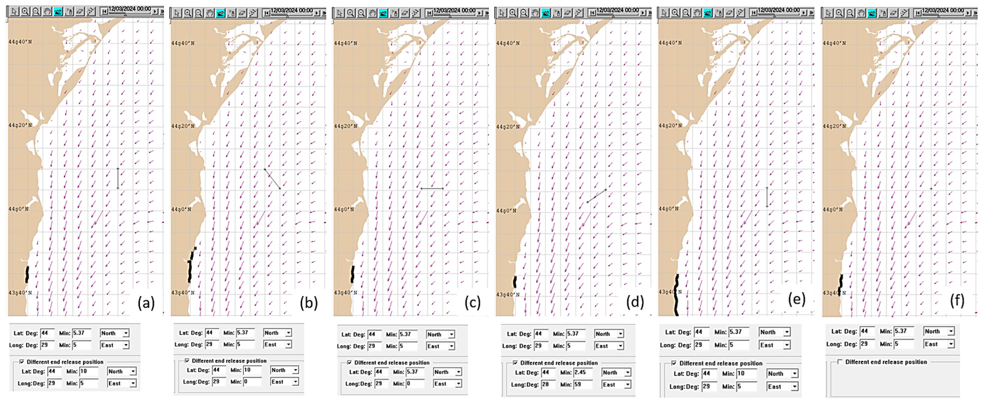
3.3. Scenario Analysis for Medium Crude Oil—Dynamic Simulation

The pollutant hazardous spillage occurred during a 24 h’ time span and the polluting source discharged 10,000 metric tons of medium crude oil, being dynamic (in movement) during this time interval. The modelling conditions introduced in the GNOME program by the authors are presented in Figure 13, simulating a situation where a ship is leaking medium crude oil being unstable and potentially under movement during this time interval, influenced by a combination of drift and by engines capability to assure the ships’ propulsion. Although the vessel’s heading was not explicitly predefined in the simulation setup, the trajectory of the resulting oil slick, as illustrated in Figure 12, provides a clear indication of directional displacement. The slick advances progressively in a southeastward arc, consistent with an estimated drift vector of approximately 110°–130° from true North. This simulated movement aligns with prevailing wind and surface current patterns along the western Black Sea coastline and mirrors typical navigational routes of outbound tankers departing from the Port of Constanța. The inferred drift direction plays a significant role in shoreline impact prediction and underlines the importance of accurately modeling vessel trajectory in dynamic oil spill assessments.

The time evolution of this scenario is illustrated in Figure 14. As observed, a larger coastal area is impacted by the oil spill due to two primary factors:

-

the spill does not occur instantaneously, but rather over an extended time interval;

-

the source of the spill (i.e., the damaged vessel) is also in motion, leading to a broader distribution of hydrocarbons.

In this case, the response effort is more complex and resource-intensive, as the affected area is significantly larger. Therefore, an optimal intervention strategy involves the early identification of the vessel’s location and the mitigation of the spill at its source, if feasible. As observed in Figure 14, when the spill occurs over an extended time interval, the affected coastal area requiring cleanup is significantly larger compared to a single instantaneous discharge. This prolonged release leads to wider dispersion and increased shoreline contamination, necessitating a more extensive and resource-intensive response effort.

Figure 15 presents a comparative analysis of hydrocarbon deposition along the coastline, categorized by oil type, four days post-spill. The results indicate that for light gasoline, the oil slicks completely evaporate within this timeframe. However, an interesting observation is that for aviation fuel, approximately 5% of the spill remains un-evaporated after four days. In the case of diesel fuel, the percentage of hydrocarbons reaching the shore after four days is measured at 40.6%. For heavier hydrocarbons, such as crude oil and no. 6 fuel oil, the residual percentages are 63% and 71.7%, respectively. This behaviour is attributed to their lower volatility and dispersion rates compared to diesel or gasoline. Thus, for hydrocarbons such as diesel and heavier oil fractions, a rapid response is imperative to contain and mitigate the oil slick, preventing long-term environmental impact.

Factually, the spatial distribution of the oil slick after four days has been analysed in Figure 15, for four different hydrocarbon types: aviation fuel, diesel, medium crude oil, and heavy hydrocarbons (Oil #6). The residual fuel oil/bunker oil (Oil #6) is a very heavy residual oil, with highest viscosity, that contains high levels of asphaltenes and waxes, requiring preheating to flow or be pumped, being used mostly in large marine engines and industrial furnaces—tends to persist in the environment, sinks or emulsifies, solidifying below ~25 °C, so more difficult to clean.

The spill conditions remain consistent with those presented in Figure 14. The analysis also includes the quantities of hydrocarbons remaining in the water, those reaching the shoreline, and those that have been dispersed or evaporated over this timeframe.

As previously mentioned, some simulations considered a non-instantaneous oil spill where the spilling vessel moves over a certain distance during the discharge. This scenario simulates a damaged vessel experiencing a continuous oil leak, which is not necessarily anchored and may undergo drift, due to currents or intentional movement powered by its engines. Understanding the optimal movement direction of the vessel can be crucial in minimizing the length of the shoreline affected by the oil slick. To explore this scenario, the authors have conducted a simulation of a 20,000-metric-ton spill of Oil #4, varying the vessel’s drift direction. Oil #4 (Intermediate Fuel Oil/Marine Diesel Blend) is defined by a blend of distillate and residual oils, lighter than residual fuel oil, more flowable at ambient temps, used in smaller marine engines or powerplants—some components evaporate, others emulsify and is less persistent but still considered moderately heavy.

In this simulation scenario the oil spill duration was set to 8 h and the initial position of the vessel was kept constant, while the final position varied to simulate different movement trajectories. This scenario also accounts for deliberate vessel movement (either under its own propulsion or being towed), considering that weather conditions, wind, and marine currents can influence the extent of shoreline contamination and help mitigate environmental impact. The simulation results are illustrated in Figure 16, displaying images (a)–(e), which show the oil slick’s evolution after two days. For comparison, the scenario where the vessel remains stationary for the entire 8-h spill duration is also included.

Further details regarding the simulation parameters used in Figure 16 are provided in Figure 17. As seen in Figure 16, the length of the shoreline impacted by the oil slick is highly dependent on the vessel’s drift direction. Is significant to notice that graphs illustrate an optimal movement direction in which the shoreline exposure is minimized compared to the stationary scenario as observed in Figure 16f, this finding suggesting that in certain conditions, controlled vessel movement during a spill may reduce the overall environmental impact on coastal areas.

The distribution of the oil slick after two days is analysed based on the drift or movement direction of the leaking vessel. The initial spill location is represented in Figure 16 as a black line or a point (for the rightmost image), while the extent of the oil slick reaching the shoreline after two days is also depicted.

4. Simulation of Oil Spill Incidents: Case Study

4.1. Simulation of Multiple Oil Spill Incidents in the Western Black Sea Area

In the final phase of the simulation analysis the authors approached the model development for multiple hydrocarbon spill scenarios to assess their impact on the shoreline, particularly whether it may affect critical infrastructure. The total simulation duration is set to 39 h (1 day and 15 h). As observed, over this period, approximately 45% of the spilled diesel evaporates or emulsifies, meaning that slightly more than half of the initially released quantity reaches the shoreline after 39 h.

The hydrocarbon chosen for this study is diesel fuel, and the spilling vessel is assumed to remain stationary throughout the simulation, while the total spill duration is 2 h, representing either: a severe vessel accident where the ship sinks within this timeframe, or the time required to stop the diesel leak from the vessel. The total amount of diesel released during this period is 15,000 metric tons.

After simulation, Figure 18 illustrates eight different spill scenarios, each representing different initial spill locations and their respective shoreline impact zones where the diesel slick reaches the coast. The results indicate that the extent of the affected shoreline varies depending on the angle of impact, and on how parallel the hydrocarbon slick may relatively move to the coastline. It is evident that critical infrastructure zones are at significant risk from such spills, emphasizing the need for effective mitigation strategies.

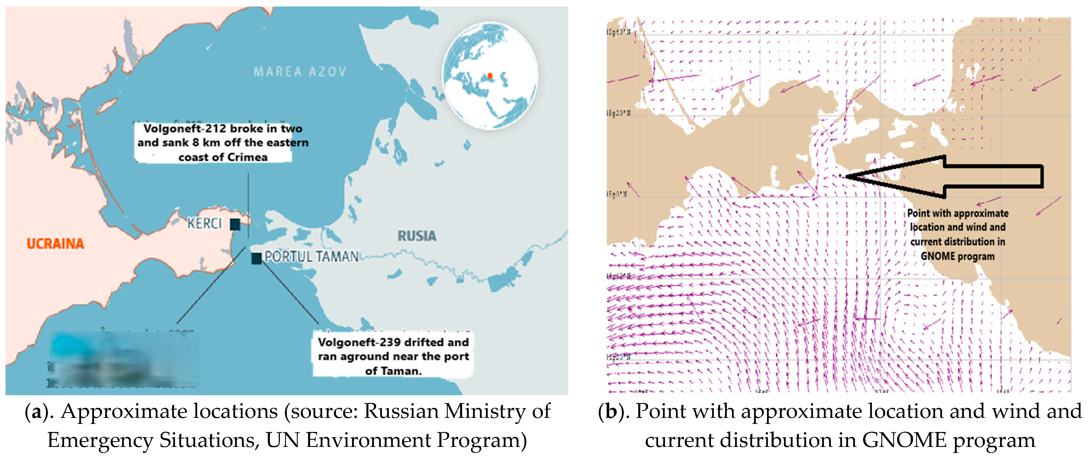
4.2. Simulation of Oil Spill Incident in Kerch Strait (Black Sea, December 2024)

On December 15, 2024, reports emerged that two oil tankers, Volgoneft-212 and Volgoneft-239, were sinking in the Kerch Strait [36]. At the time of the incident, state media reported that both vessels, each over 50 years old, were carrying a combined cargo of approximately 62,000 barrels (9200 metric tons) of petroleum products [37]. However, the true extent of the environmental disaster was later found to be more severe than initially acknowledged by the authorities. During a severe storm, Volgoneft-212 reportedly broke in two and sank, while Volgoneft-239 ran aground. By December 17, oil slicks had reached the Anapa coastline and Temryuk district in Russia’s Krasnodar Krai. According to the Russian Ministry of Transport, approximately 2400 metric tons of heavy fuel oil were discharged into the Black Sea as a result of the damage. Of the total 9200 tons of petroleum cargo, an estimated 5000 tons of fuel oil settled on the seabed, forming what regional Governor Veniamin Kondratiev described as a “gelatinous mass that remains stationary on the seafloor [38].

Based on preliminary data (type, quantity, and location of the spill), a post-pollution simulation scenario was developed for the Volgoneft-239 incident, assuming the release of 4000 tons of heavy fuel oil. Using the GNOME v.47.2 modeling system and period-matched hydro-meteorological data, simulation results were generated and presented in hourly intervals (see Figure 19).

The simulation outcomes validated media-reported observations from this real-world case study: the trajectory and geographic distribution of the affected zones in the Kerch Strait were consistent with the model’s predictions. In the initial days following the incident, lighter petroleum fractions (e.g., diesel) reached the predicted areas within the estimated time frame. Approximately one month later, heavier fuel oil fractions, transported by subsurface currents, began making landfall. Subsequent reports confirmed a new wave of fuel oil pollution discovered on Sunday, January 12, impacting a wider area, including the municipalities of Yevpatoria, Sudak, Feodosia, Yalta, as well as the Saky and Chornomorske districts, Tuzla Island, and Cape Takil in the Lenine District. Official agencies deployed 225 monitoring teams, 22 response vessels, and aerial surveillance via two Mi-8 helicopters to track and mitigate the movement of the spill (https://www.euractiv.ro, accessed on 1 December 2024). These developments highlight the urgent need for future research to focus on the deep-water dispersion dynamics of heavier hydrocarbon fractions, which may persist in the marine environment long after the initial event and pose ongoing risks to coastal ecosystems.

Based on the analyses presented—including the Kerch Strait case study—it is evident that the primary factors influencing hydrocarbon transport and dispersion in the marine environment are:

-

the nature of the spilled hydrocarbon, including its density, viscosity, and chemical composition;

-

hydro-meteorological parameters, such as surface and subsurface currents, wind speed and direction, wave height, and tidal activity;

-

the physicochemical properties of seawater, including temperature, salinity, and the presence of suspended particles (notably terrigenous particles transported by nearby rivers, which can enhance the adhesion and sedimentation of heavier hydrocarbon fractions);

-

the presence of algal blooms, which can exert a similar effect to suspended particulate matter, influencing hydrocarbon aggregation and distribution.

Each of these factor categories can interact and influence one another to varying degrees. For example, in the case of fuel oil discharge in the Kerch Strait, subsurface currents and low water temperatures played a critical role in the spill’s behavior. Unlike lighter crude oils that float and spread across the water surface, fuel oil tends to solidify below 25 °C, making it significantly more difficult to recover. Once solidified, it becomes neutrally or negatively buoyant and may sink or remain suspended at varying depths, eventually being transported by deep-water currents to remote coastal zones or seafloor accumulation sites.

This scenario demonstrates the need for predictive mathematical models that incorporate vertical distribution of environmental parameters and hydrocarbon-specific behaviors. Such models must account for interactions between hydrocarbon type, oceanographic conditions, and the local marine environment to enable accurate forecasting of pollutant trajectories and inform timely, targeted response strategies.

5. Conclusions

This study presents a comprehensive approach to oil spill drift modelling, utilizing two advanced simulation tools: GNOME v.47.2 (General NOAA Operational Modelling Environment) and ADIOS2 v.2.10.2 (Automated Data Inquiry for Oil Spills). The research focuses on the Romanian Black Sea coast and evaluates different spill scenarios to enhance response strategies.

The key findings of present research are outlined as following:

a. Integration of real-time environmental data enhances predictive accuracy.

-

the study demonstrates that incorporating real-time meteorological and oceanographic data significantly improves simulation outcomes, making spill trajectory forecasts more reliable;

-

GNOME’s ability to dynamically adjust hydrodynamic parameters (wind, currents, tides) enables detailed scenario analysis.

b. Oil type influences spill evolution and environmental impact.

-

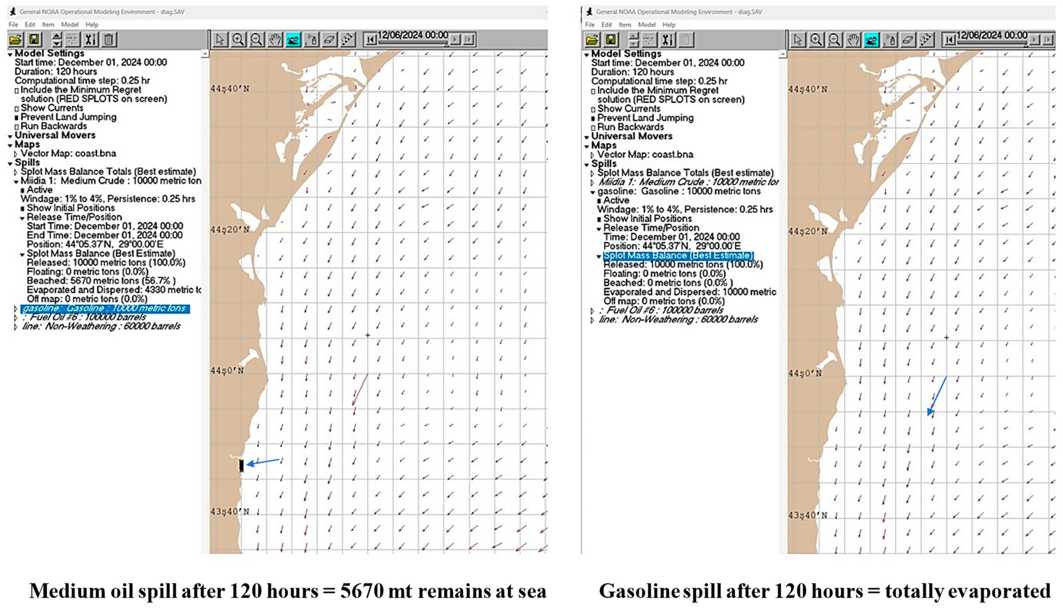
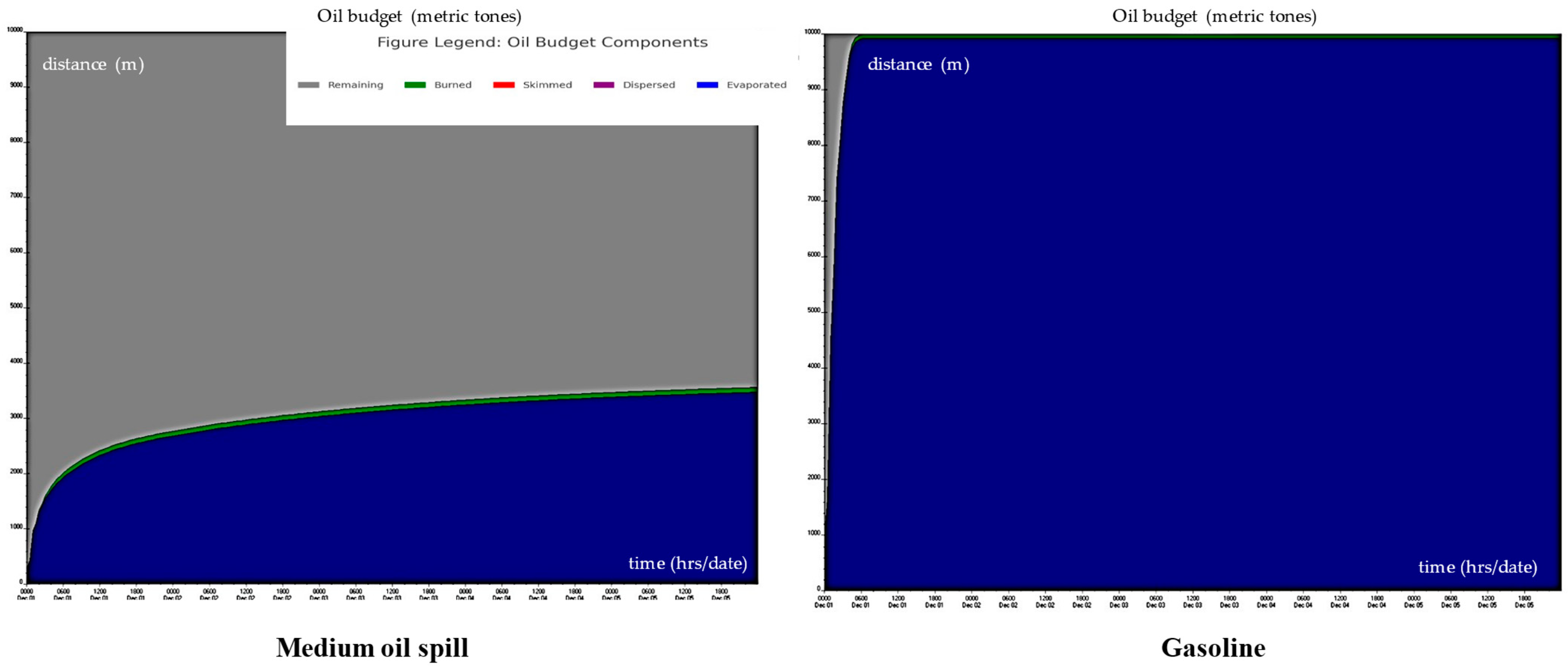
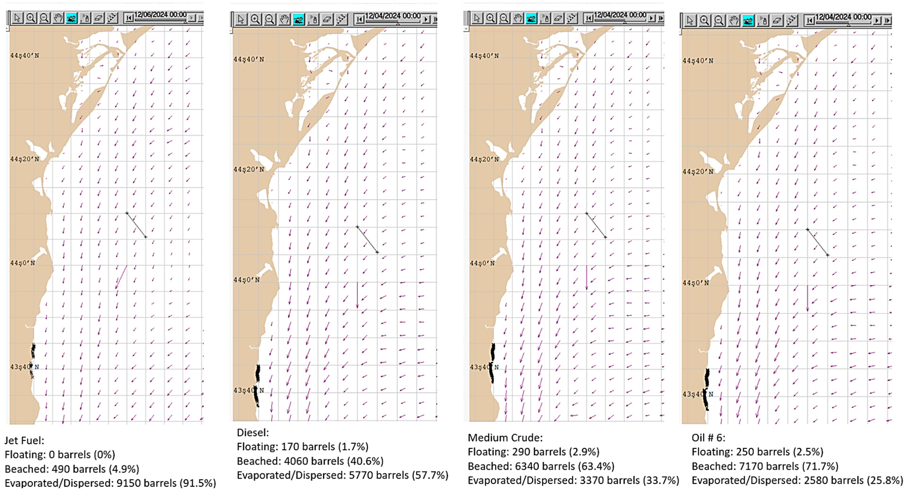
lighter hydrocarbons (e.g., gasoline, aviation fuel) evaporate quickly, reducing the amount of pollutant reaching the shoreline;

-

heavier hydrocarbons (e.g., crude oil, fuel oil #6) persist longer in the marine environment and require mechanical recovery and intervention;

-

after four days post-spill, gasoline evaporates completely, while 63–71.7% of heavier oil fractions remain in the water or along the coast.

c. Static vs. dynamic spill sources affect shoreline contamination differently.

-

stationary spills create more localized contamination, while moving sources (e.g., damaged vessels drifting) cause a broader environmental impact;

-

the study shows that controlling the drift direction of a leaking vessel can help minimize the affected shoreline area.

d. Early intervention is crucial for reducing long-term environmental damage.

-

using ADIOS software, the study evaluates various mitigation techniques, including: dispersants for breaking down oil slicks, skimming techniques for mechanical recovery, controlled burning to eliminate surface oil;

-

the findings emphasize the importance of rapid response to prevent oil from reaching sensitive infrastructure and ecosystems.

e. Risk to critical infrastructure is significant.

-

the modelling results highlight that oil spills can impact critical coastal infrastructure, including ports (Constanța and Midia) and economic zones;

-

the risk varies depending on spill location, type of hydrocarbon, and environmental conditions;

The study provides practical advancements in oil spill modelling and response planning, including:

-

refinement of GNOME and ADIOS2 v.2.10.2 integration for oil spill trajectory and impact assessment.

-

identification of optimal intervention strategies based on real-time environmental data.

-

new insights into the relationship between spill duration, vessel movement, and shoreline contamination.

Based on the study’s findings, several key recommendations can be made to improve oil spill response strategies and environmental protection:

a. Improving Real-Time Monitoring and Data Integration

-

expand the use of remote sensing technology (e.g., satellites, drones, and real-time buoys) to enhance data accuracy for GNOME v.47.2 simulations;

-

develop automated data assimilation techniques to continuously update models with real-time meteorological and oceanographic inputs.

b. Enhancing Oil Spill Response Strategies

-

prioritize rapid response for heavier hydrocarbons, as they pose the greatest environmental threat due to their persistence;

-

implement vessel movement strategies to reduce shoreline contamination when a spill occurs from a drifting source;

-

increase response preparedness near critical infrastructure (e.g., ports, pipelines, economic hubs).

c. Policy and Management Recommendations

-

develop region-specific intervention plans based on the type of hydrocarbons most likely to be spilled;

-

enhance cross-border coordination among Black Sea nations to share real-time data and response capabilities;

-

enforce stricter regulations for maritime traffic and offshore oil operations to minimize spill risks.

d. Future Research Directions

-

integrate AI and machine learning to improve oil spill prediction models;

-

develop enhanced numerical models for complex spill scenarios (e.g., deepwater spills, Arctic conditions);

-

refine mitigation techniques for reducing the environmental impact of heavier hydrocarbons.

This study successfully demonstrates the effectiveness of GNOME v.47.2 and ADIOS2 v.2.10.2 in oil spill prediction and response planning. By combining real-time data, numerical modeling, and scenario analysis, the authors provide a valuable contribution to oil spill management in the Black Sea region. Their work highlights the critical need for proactive measures, early intervention, and technological advancements in oil spill response to protect coastal infrastructure and marine ecosystems.

6. Authors’ Contribution

This research contributes to the advancement of oil spill simulation methodologies by integrating hydrodynamic trajectory models with chemical weathering analysis. The study enhances existing knowledge on spill evolution under real-time environmental conditions, offering a practical framework for risk assessment and mitigation strategies in marine environments.

References

1. Toz, A.C.; Buber, M. Performance evaluation of oil spill software systems in early fate and trajectory of oil spill: Comparison analysis of OILMAP and PISCES 2 in Mersin bay spill. Environ. Monit. Assess. 2018, 190, 551. [Google Scholar] [CrossRef] [PubMed]
2. Barreto, F.T.; Dammann, D.O.; Tessarolo, L.F.; Skancke, J.; Keghouche, I.; Innocentini, V.; Winther-Kaland, N.; Marton, L. Comparison of the Coupled Model for Oil spill Prediction (CMOP) and the Oil Spill Contingency and Response model (OSCAR) during the DeepSpill field experiment. Ocean. Coast. Manag. 2021, 204, 105552. [Google Scholar] [CrossRef]
3. Soussi, A.; Bersani, C.; Tomasoni, A.M. Oil spill trajectory: A comparison between 2D and 3D models. Urban Marit. Transp. XXVII 2021, 204, 117–128. [Google Scholar] [CrossRef]
4. Zacharias, D.C.; Lemos, A.T.; Keramea, P.; Dantas, R.C.; da Rocha, R.P.; Crespo, N.M.; Sylaios, G.; Jovane, L.; da Silva Santos, I.G.; Montone, R.C.; et al. Offshore oil spills in Brazil: An extensive review and further development. Mar. Pollut. Bull. 2024, 205, 116663. [Google Scholar] [CrossRef] [PubMed]
5. Longhi, R.P.; Ferreira Filho, V.J. Strategic location model for oil spill response vessels (OSRVs) considering oil transportation and weather uncertainties. Mar. Pollut. Bull. 2024, 207, 116829. [Google Scholar] [CrossRef] [PubMed]
6. Dhaka, A.; Chattopadhyay, P. A review on physical remediation techniques for treatment of marine oil spills. J. Environ. Manag. 2021, 288, 112428. [Google Scholar] [CrossRef] [PubMed]
7. Zhu, Z.; Merlin, F.; Yang, M.; Lee, K.; Chen, B.; Liu, B.; Cao, Y.; Song, X.; Ye, X.; Li, Q.K.; et al. Recent advances in chemical and biological degradation of spilled oil: A review of dispersants application in the marine environment. J. Hazard. Mater. 2022, 436, 129260. [Google Scholar] [CrossRef] [PubMed]
8. Bhardwaj, S. Developing and Evaluating Novel Solutions to Understand the I/O Bottlenecks in HPC Applications. University of Edinburgh. 2024. Available online: https://era.ed.ac.uk/bitstream/handle/1842/42870/Bhardwaj2024.pdf (accessed on 30 November 2024).
9. Bi, B.; Guan, Y.; Qiao, D.; Chen, X.; Bao, M.; Wang, Z.; Li, Y. MXene/Graphene modified cellulose aerogel for photo-electro-assisted all-weather cleanup of high-viscous crude oil from spill. J. Hazard. Mater. 2023, 460, 132353. [Google Scholar] [CrossRef] [PubMed]
10. Wei, Z.; Wei, Y.; Liu, Y.; Niu, S.; Xu, Y.; Park, J.-H.; Wang, J.J. Biochar-based materials as remediation strategy in petroleum hydrocarbon-contaminated soil and water: Performances, mechanisms, and environmental impact. J. Environ. Sci. 2024, 138, 350–372. [Google Scholar] [CrossRef] [PubMed]
11. Mahmood, R.M. Trajectory modelling of oil spills: Comparing GNOME and ADIOS2 performance in offshore environments. Environ. Fluid Dyn. J. 2024, 29, 421–437. [Google Scholar]
12. NOAA. Deepwater Horizon Response: Oil Spill Trajectory Forecasting Using GNOME; NOAA Technical Report; NOAA: Washington, DC, USA, 2011.
13. Galt, J.A.; Lehr, W.J.; Payton, D. GNOME: A review of operational applications for oil spill trajectory modelling. Mar. Pollut. Bull. 2022, 84, 267–280. [Google Scholar]
14. Lame, N.G.; Mahmood, R.M. Oil Spill Fate and Trajectory Simulation for the Buzzard Oilfield, Outer Moray Firth, United Kingdom. ResearchGate. 2024. Available online: https://www.researchgate.net/publication/384043781_OIL_SPILL_FATE_AND_TRAJECTORY_SIMULATION_FOR_THE_BUZZARD_OILFIELD_OUTER_MORAY_FIRTH_ABERDEEN_UNITED_KINGDOM (accessed on 30 November 2024).
15. Güven, B. Combining GNOME and ADIOS2 for more accurate oil spill fate predictions. J. Environ. Monit. 2021, 13, 553–568. [Google Scholar]
16. Zarochtunnisa, A.I.; Ludina, Y.M.; Ardhiani, N.E. SNAP dan General NOAA Oil Modeling Environment (GNOME) untuk Deteksi Sebaran Tumpahan Minyak (Oil Spill) di Selat Madura. Majalah Ilmiah. 2024. Available online: https://core.ac.uk/download/pdf/628397933.pdf (accessed on 30 November 2024).
17. Zelenke, B.; O’Connor, C.; Barker, C.H.; Beegle-Krause, C.; Eclipse, L. Advancements in real-time oil spill forecasting with GNOME. J. Mar. Sci. Eng. 2012, 1, 67–82. [Google Scholar]
18. Galt, J. Trajectory analysis for oil spills. Mar. Pollut. Bull. 1995, 30, 145–152. [Google Scholar]
19. Sarker, S. Separation of Floodplain Flow and Bankfull Discharge: Application of 1D Momentum Equation Solver and MIKE 21C. CivilEng 2023, 4, 933–948. [Google Scholar] [CrossRef]
20. Mezali, F.; Benmamar, S.; Naima, K.; Ameur, H. Evaluation of Stent Effect and Thrombosis Generation with Different Blood Rheology on an Intracranial Aneurysm by the Lattice Boltzmann Method. ScienceDirect. 2022. Available online: https://www.sciencedirect.com/science/article/abs/pii/S0169260722001432 (accessed on 30 November 2024).
21. Yang, L.; Xie, L.; You, J.; Liang, P.; Zhang, T. Mechanisms of Intraseasonal Oscillation in Equatorial Surface Currents in the Pacific Ocean Identified by Neural Network Models. 2025. Available online: https://agupubs.onlinelibrary.wiley.com/doi/abs/10.1029/2024JC021514 (accessed on 30 November 2024).
22. Harris, E. Drivers of Warm Water Variability in Atlantic Hurricane Regions. Ph.D. Thesis, University of Southampton, Southampton, UK, 2025; 109p. Available online: https://eprints.soton.ac.uk/497885 (accessed on 30 November 2024).
23. Huang, W.; Li, C.; Rivera-Monroy, V.H. Cold fronts control multiscale spatiotemporal hydroperiod patterns in a man-made subtropical coastal delta (Wax Lake Region, Louisiana USA). Ocean Dyn. 2024, 74, 355–372. [Google Scholar] [CrossRef]
24. Feizabadi, S.; Li, C.; Hiatt, M. A numerical experiment of cold front-induced circulation in Wax Lake Delta: Evaluation of forcing factors. Sec. Phys. Oceanogr. 2023, 10, 1228446. [Google Scholar] [CrossRef]
25. Cernuda, J.; Logan, L.; Gainaru, A.; Klasky, S.; Lofstead, J.; Kougkas, A.; Sun, X.H. Hades: A context-aware active storage framework for accelerating large-scale data analysis. In Proceedings of the 2024 IEEE 24th International Symposium on Cluster, Cloud and Internet Computing (CCGrid), Philadelphia, PA, USA, 6–9 May 2024; Available online: https://www.osti.gov/servlets/purl/2441008 (accessed on 30 November 2024).
26. Williams, J.J.; Medeiros, D.; Costea, S.; Tskhakaya, D.; Poeschel, F.; Widera, R.; Huebl, A.; Klasky, S.; Podhorszki, N.; Kos, L.; et al. Enabling High-Throughput Parallel I/O in Particle-in-Cell Monte Carlo Simulations with openPMD and Darshan I/O Monitoring. IEEE Cluster Computing. 2024. Available online: https://arxiv.org/pdf/2408.02869 (accessed on 30 November 2024).
27. Duwe, K.; Kuhn, M. DAI: How Pre-Computation Speeds up Data Analysis. International Conference on Computational Science. 2024. Available online: https://www.iccs-meeting.org/archive/iccs2024/papers/148330106.pdf (accessed on 30 November 2024).
28. Song, Y.; Li, Y.; Li, G.; Liu, Y.; Wu, T.; Yin, S.; Xue, W.; Wang, J. A Data Optimizer for Region-Aware Self-describing Files in Scientific Computing. ACM Cloud Computing Conference. 2024. Available online: https://dl.acm.org/doi/pdf/10.1145/3698038.3698526 (accessed on 30 November 2024).
29. Efendi, E.J. Methods of Oil Spill Cleanup: A Comparative Review. In Proceedings of the Offshore Technology Conference, Houston, TX, USA, 9 May 2024. [Google Scholar] [CrossRef]
30. Fingas, M. Oil Spill Science and Technology; Elsevier: Amsterdam, The Netherlands, 2016. [Google Scholar]
31. Johansen, Ø.; Brandvik, P.J.; Farooq, U. Challenges in deepwater oil spill modelling: A review of existing approaches and future directions. Mar. Environ. Res. 2023, 112, 104865. [Google Scholar]
32. Lehr, W.J.; Simecek-Beatty, D. Shoreline Impact Modelling of Oil Spills Using GNOME and ADIOS2; NOAA Technical Report; NOAA: Washington, DC, USA, 2020. [Google Scholar]
33. Lehr, W.; Simecek-Beatty, D. The ADIOS oil spill model: A decision support tool. Environ. Model. Softw. 2000, 15, 125–134. [Google Scholar]
34. National Oceanic and Atmospheric Administration (NOAA). GNOME User Manual. Available online: https://gnome.orr.noaa.gov (accessed on 30 November 2024).
35. Scutaru, G. Black Sea’s Offshore Energy Potential and Its Strategic Role at a Regional and Continental Level. New Strategy Center, Bucharest. 2024. Available online: https://newstrategycenter.ro/wp-content/uploads/2024/03/Studiu-Kas-Black-Sea-final-version.pdf (accessed on 30 November 2024).
36. Available online: https://www.defenseromania.ro/la-limita-unui-dezastru-ecologic-major-in-marea-neagra-petrolierele-rusesti-reprezinta-o-amenintare-pentru-mediu-rusia-foloseste-nave-foarte-vechi-de-50-de-an_631757.html (accessed on 24 December 2024).
37. Available online: https://www.digi24.ro/stiri/externe/pata-de-petrol-din-stramtoarea-kerci-a-ajuns-pe-coasta-marii-azov-3076655 (accessed on 11 January 2025).
38. Available online: https://www.euractiv.ro/eu-elections-2019/pacura-de-la-petrolierele-rusesti-de-langa-kerci-se-strange-cu-lopeti-70759 (accessed on 30 November 2024).
Figure 1. Map of critical structure on Black Sea with focus on Western region (Source: authors’ processing based on Romanian Maritime Hydrographic Directorate data base, combined with Scutaru G., 2024 [35]).
Sustainability 17 03770 g001
Figure 2. Initial stage of simulation—red square area marks the selection of studied map from dedicated websites (Source: https://gnome.orr.noaa.gov/goods/tools/GSHHS/coast_subset, accessed on 30 November 2024).
Sustainability 17 03770 g002
Figure 3. Real-time wind and marine currents data retrieved by inputting the geographic coordinates—red square marks the selection of studied map (Source: authors’ processing, using the retrieved data from https://gnome.orr.noaa.gov/goods/currents/HYCOM/get_data, accessed on 30 November 2024).
Sustainability 17 03770 g003
Figure 4. Weather context at the beginning of oil and hydrocarbon spill simulations—the arrows are indicating the direction of sea currents (Source: authors’ processed print screen from specialized online platforms).
Sustainability 17 03770 g004
Figure 5. GNOME parameters used in the simulation of medium oil spill evolution in the Black Sea region, on selected date (1 December 2024), using real-time conditions for wind and sea currents (Source: authors’ processed print screen during parameters from NOOA website uploaded in GNOME v.47.2 software).
Sustainability 17 03770 g005
Figure 6. Medium oil spills dynamics in time evolution in Western Black Sea area—the blue arrows indicate the oil spill position, while smaller arrows indicate the direction of sea currents (Source: authors’ processed data on GNOME v.47.2 software, dated on 1 December 2024).
Sustainability 17 03770 g006
Figure 7. The time evolution of an oil slick depending on the evaporated, dispersed and extracted share of pollutant, during the intervention, predicted by the ADIOS2 v.2.10.2 code (Source: authors’ processed data on ADIOS2 v.2.10.2 software).
Sustainability 17 03770 g007
Figure 8. Time evolution of an oil slick predicted by ADIOS2 v.2.10.2, for each individual component—left upper side N/A represents the ”blank” initiation screen (Source: authors’ processed data on ADIOS2 v.2.10.2 software).
Sustainability 17 03770 g008
Figure 9. Time evolution in case of oil spill predicted by ADIOS2 v.2.10.2, valuing the data from Figure 6 (Source: authors’ processed data on ADIOS2 v.2.10.2 software).
Sustainability 17 03770 g009
Figure 10. Gasoline spills dynamics in time evolution in Western Black Sea area—the blue arrows indicate the oil spill position, while smaller arrows indicate the direction of sea currents (Source: authors’ processed data on GNOME v.47.2 software, dated on 1 December 2024).
Sustainability 17 03770 g010
Figure 11. The predicted quantity and location of spilled hydrocarbon layer at sea 120 h after the spill—the blue arrows indicate the oil spill position, while smaller arrows indicate the direction of sea currents (Source: authors’ processed data on GNOME v.47.2 software).
Sustainability 17 03770 g011
Figure 12. Evolution in time for hydrocarbon spill predicted by ADIOS2 v.2.10.2 software (oil spill in left image and gasoline in the right image) (Source: authors’ processed data on ADIOS2 v.2.10.2 software).
Sustainability 17 03770 g012
Figure 13. Oil spill simulation for a moving source and progressive spillage scenario (Source: authors’ processed data on GNOME v.47.2 software).
Sustainability 17 03770 g013
Figure 14. Temporal evolution of the oil spill location—the oil spill positions are marked in black lines, while the arrows are indicating the direction of sea currents (Source: authors’ processed data on GNOME v.47.2 software).
Sustainability 17 03770 g014
Figure 15. Oil slick location four days post-spill for different hydrocarbon types—the oils spill is marked in black lines, while the arrows are indicating the direction of sea currents (Source: authors’ processed data on GNOME v.47.2 software).
Sustainability 17 03770 g015
Figure 16. Oil slick location two days post-spill, modelled in relation with drift direction of spill source—the oils spill are marked ashore in black color, while the arrows are indicating the direction of sea currents. Moreover, the positions of oil spill are established indicating the their coordinates in the table provided under each image (Source: authors’ processed data on GNOME v.47.2 software).
Sustainability 17 03770 g016
Figure 17. Detailed parameters and simulation conditions for scenario model from Figure 16 (Source: authors’ processed data on GNOME v.47.2 software).
Sustainability 17 03770 g017
Figure 18. Multiple initial spill conditions (blue star symbol) and corresponding shoreline impacting locations—the arrows represent the sea currents, the stars positions represent the initial spill locations, while the black shapes mark the shore impact location (Source: authors’ processed data on GNOME v.47.2 software).
Sustainability 17 03770 g018
Figure 19. Post-pollution simulation scenario for oil tanker Vol-goneft-239 in the onboard spill incident of 4000 tons of fuel oil—the arrows are indicating the sea currents evolutions (Source: authors’ processed data on GNOME v.47.2 software).
Sustainability 17 03770 g019aSustainability 17 03770 g019b
Disclaimer/Publisher’s Note: The statements, opinions and data contained in all publications are solely those of the individual author(s) and contributor(s) and not of MDPI and/or the editor(s). MDPI and/or the editor(s) disclaim responsibility for any injury to people or property resulting from any ideas, methods, instructions or products referred to in the content.