Sustainable Shipping: Modeling Economic and Greenhouse Gas Impacts of Decarbonization Policies (Part II)

Abstract

Maritime transport carries over 80% of global trade by volume and remains the most energy-efficient mode for long-distance goods movement. However, the sector contributes approximately 3% of global Greenhouse Gas (GHG) emissions, a share that could rise to 17% by 2050 without effective regulation. In response, the International Maritime Organization (IMO) has introduced initial and short-term measures to enhance energy efficiency and reduce emissions. In 2023, IMO Strategy expanded on these efforts with medium-term measures, including Market-Based Mechanisms (MBMs) such as a GHG levy, a feebate system, and fuel intensity regulations combined with carbon pricing. This study evaluates the economic and environmental impacts of these measures using an integrated computational simulation model that combines Ocean Engineering and Economics. Our results indicate that all proposed measures support the IMO’s intermediate emission reduction targets through 2035, cutting absolute emissions by more than 50%. However, economic impacts vary significantly across regions, with most of Africa, Asia, and South America experiencing the greatest adverse effects on GDP and trade. Among the measures, the GHG levy exerts the strongest pressure on economic activity and food prices, while a revised fuel intensity mechanism imposes lower costs, particularly in the short term. Revenue redistribution mitigates GDP losses but does so unevenly across regions. By leveraging a general equilibrium model (GTAP) to capture indirect effects often overlooked in prior studies, this analysis provides a comprehensive comparison of policy impacts. The findings underscore the need for equitable and pragmatic decarbonization strategies in the maritime sector, contributing to ongoing IMO policy discussions.

1. Introduction

Maritime transport was responsible for more than 80% of the total volume of world trade in 2019, playing a crucial role in global supply chain. It is the dominant mode for transporting strategic raw materials, such as grains, crude oil, and iron ore, as well as chemicals and refined fuels, supporting economic development worldwide. Despite being the most energy-efficient mode of transport over long distances, with lower carbon emissions per tonne-mile compared to road and air transport, the shipping sector remains a major contributor to global Greenhouse Gas (GHG) emissions, accounting for approximately 3% of global emissions. If left unregulated, emissions from shipping could rise to 17% by 2050 [1] as international trade volumes continue to expand (The volume of international maritime trade increased from 7857 million tons (Mt) in 2009 to 11,005 Mt in 2018 [2]. This growth path was interrupted during the COVID-19 pandemic years but recovered in 2021).

To address this challenge, the International Maritime Organization (IMO) has taken a leading role in regulating emissions from maritime transport, particularly since the sector was not initially covered by the Paris Agreement. In 2023, IMO member states revised their initial strategy, now aiming for net zero emissions by 2050 (In 2018, IMO members adopted an initial strategy aiming to reduce the sector’s absolute GHG emissions by 50% by 2050 compared to 2008 levels, with a subsequent revision in 2023 to achieve net zero emissions by 2050 [3]). Initial and short-term measures—such as the Energy Efficiency Existing Ship Index (EEXI) and the Carbon Intensity Indicator (CII)—were introduced in November 2022 to improve energy efficiency in vessels (These regulations have driven the maritime sector to invest significantly in new technologies and infrastructure, such as cleaner engines, hybrid propulsion, optimized hull design, and efficient navigation practices. These changes, though necessary, increase operational and capital costs in maritime transport, which requires international cooperation to ensure their effectiveness and global compliance). However, achieving long-term decarbonization requires additional regulatory and market-based mechanisms (MBMs). Among the MBMs under discussion are a GHG levy, a fuel-intensity-based flexible mechanism (GHG Fuel Intensity, GFI), and a feebate system. These policies aim to create economic incentives for emissions reductions, but their potential economic and environmental impacts remain uncertain.

This study evaluates the economic and environmental effects of the proposed medium-term measures, considering their interaction with existing policies (required levels of EEXI and CII) from 2023 to 2035. To achieve this, we integrate two complementary modeling approaches: an ocean engineering model to estimate the impact of new policies on maritime transport costs and an economic model (the Global Trade Analysis Project, GTAP) to assess the broader economic implications. The GTAP is particularly suitable for this analysis because it captures both direct and indirect economic effects across multiple regions and sectors, including trade shifts and price adjustments, which are critical for assessing the distributional impacts of carbon pricing policies (The GTAP model is widely used for assessing trade and environmental policies due to its ability to incorporate multiple sectors and global linkages, providing a comprehensive perspective on policy-induced changes. However, its reliance on strong assumptions—such as market-clearing conditions and representative agent behavior—may limit its applicability in contexts with structural rigidities or imperfect competition. Additionally, GTAP databases are updated less frequently than the data used in partial equilibrium approaches, potentially affecting the timeliness of results. Despite these limitations, the general equilibrium framework is particularly useful for dynamic analysis, as it captures long-term adjustments, factor mobility, and environmental and transportation responses within a consistent economic structure). Alternative modeling approaches, such as partial equilibrium models or sector-specific cost-benefit analyses, do not fully account for cross-sectoral interactions and global trade adjustments, making them less effective for evaluating policies with widespread economic repercussions.

To assess the technological feasibility and costs of decarbonization, we use a detailed engineering model that relies on various secondary and administrative datasets, including satellite data, to capture the global fleet’s technological and growth needs. This model optimizes the selection of cost-effective emissions-reduction technologies for different ship types, sizes, and ages, prioritizing options with higher adoption likelihood and technological maturity (see [4] for more details). The output of this engineering model—changes in maritime transport costs due to technological adoption—is then fed into an economic model to evaluate the broader economic implications of these cost changes.

Into the economic model employed, GTAP, we incorporate key macroeconomic projections, including population growth and total factor productivity trends, based on the Shared Socioeconomic Pathway 2 (SSP2) scenario (The SSP2 (Shared Socioeconomic Pathway 2) is referred to as the “Middle of the Road” scenario defined by UN-IPCC (United Nations’ Intergovernmental Panel on Climate Change)). This allows for a comparison between a Business-as-Usual (BAU) scenario—where no additional climate policies are implemented—and various policy intervention scenarios. In addition to conventional macroeconomic indicators such as real GDP, trade, and consumer prices, our analysis places particular emphasis on food prices and maritime GHG emissions. Furthermore, we introduce two critical maritime-specific features into the GTAP framework: (i) the possibility of substitution between transport modes, (ii) the incorporation of a slack variable to simulate maritime transport price shocks, accounting for both technological advancements and MBMs over time.

We estimate the impacts for a BAU scenario (reference) and four additional scenarios, each implementing one of the analyzed medium-term measures individually. We also simulate two additional scenarios to assess the effects of disbursing funds generated from the proposed GHG levy. One scenario considers disbursing revenue to developing countries, Small Island Developing States (SIDS), and Least Developed Countries (LDCs), while another limits revenue distribution to SIDs and LDCs only. Although the revenue disbursement in our simulations is not sector-specific, it provides important insights into how redistribution influences economic variables.

Our findings show that all analyzed medium-term measures align with the IMO intermediate GHG reduction targets through 2035, achieving absolute emissions reductions higher than 50%. However, the economic impacts of these measures vary significantly across regions, raising significant equity concerns that should be addressed in the IMO discussions and decision-making. The regions experiencing the most pronounced negative effects in terms of GDP and trade are western, south-central, and north Africa; South America; and south, southeast and western Asia.

Among the medium-term measures, some impose more severe global economic effects than others over the analysis period. The GHG levy emerges as the measure with the most significant adverse impact on economic indicators—including GDP, exports, imports, and food prices—whereas the revised GFI flexibility mechanism exhibits the least disruptive effects on economic activity and food affordability. Contrary, revenue redistribution does not offsets the overall economic losses and its mitigating effects are unevenly distributed across regions, with Africa experiencing only modest gains.

This paper contributes to the IMO’s discussion on medium-term measures by providing a comprehensive comparative analysis of the environmental and economic impacts of the proposals from member states using the general equilibrium GTAP model. While much of the existing literature focuses on carbon taxation within the maritime sector [5,6,7,8], our approach evaluates a broader range of policy measures and their economic implications. Moreover, this study highlights the value of general equilibrium models in climate policy analysis, particularly their ability to capture indirect impacts and price adjustments post policy implementation [9].

Given that GTAP was not originally designed for maritime sector analysis, this paper advances the literature by combining existing methodologies with external datasets while utilizing a global perspective. We build on prior studies that introduce equations allowing transport mode substitution between maritime and air transportation [10] and enhance the model by incorporating a slack variable to account for shifts in maritime transport costs, accommodating cost changes and technological advancements [11]. We also employ machine-learning techniques to estimate the share of international trade transported by ships in 2017, ensuring a more accurate representation of shipping emissions and the magnitude of cost shocks implemented in GTAP.

We also add to the literature on the sectoral impacts of carbon taxes, particularly those incorporating revenue recycling mechanisms. While most studies focus on market-based measures implemented at a national or regional level [12,13,14,15], our analysis provides insights into the global implications of maritime sector carbon pricing. Our findings align with existing pieces of research [16,17], which find regressive impacts of carbon taxes, even after accounting for general equilibrium effects, including source-side impacts.

Finally, our analysis highlights the need for investigating both short-term and long-term policy outcomes. While a GHG levy may be more effective in driving emissions reductions over the long term, our results indicate that it imposes disproportionately high economic costs in the short and medium term. Importantly, all the policies analyzed successfully achieve the decarbonization targets. These economic burdens are particularly severe for countries located far from major markets—mainly developing economies—and for nations where transitioning to more efficient fleets may be slower due to financial or logistical constraints. Such disparities emphasize the necessity of designing policies that balance environmental effectiveness with economic feasibility, addressing both equity and implementation challenges across different time horizons.

The paper is structured as follows: A background on the impacts of decarbonization policies, as well as on the discussions within IMO is presented in Section 2. Section 3 describes the methodology adopted to estimate the variation of maritime transport costs (Marine Engineering framework—Section 3.1) and subsequently, the application of the GTAP model to assess their impacts on GDP, exports, imports, consumer price index, food prices, and GHG emissions (Economics framework—Section 3.2). Section 4 shows the descriptive statistics for maritime costs and emissions. Section 5 presents the impacts on economic variables and GHG emissions. Section 6 and Section 7 present the discussion and final remarks, respectively.

2. Background

2.1. Decarbonization Policies

Addressing climate change is challenging due to the lack of clearly defined property rights over the atmosphere, which is treated as a shared, global public good. As [18] notes, private actors often have limited motivation to drive sustainability transitions, as the benefits of such actions are collective, leading to issues like free-riding. Given the biosphere’s limited capacity to absorb carbon emissions, regulatory intervention becomes essential. A combination of regulatory and economic measures is necessary to internalize environmental costs and drive behavioral change.

Regulatory policies establish direct mandates or restrictions, such as emission limits, technology standards, or fuel-efficiency requirements, ensuring compliance through enforcement mechanisms. In contrast, economic policies, such as carbon pricing, use market-based mechanisms to create financial incentives for emissions reductions. Carbon pricing includes carbon taxes, which impose a fixed cost per unit of emissions, and Emissions Trading Systems (ETSs), which cap total emissions and allow firms to trade allowances. Both approaches aim to encourage businesses and individuals to adopt cleaner technologies and practices by making pollution more costly/viable.

The evidence shows that decarbonization policies lower harmful emissions, though their economic impact varies. Carbon pricing mechanisms, such as carbon taxes and Emissions Trading Systems (ETSs), have shown limited effectiveness. Green [19], based on several ex-post analyses, finds that carbon taxes reduce emissions by an average of 0–2% per year, while ETSs achieve reductions of 0–1.5% annually, with significant variation across sectors. Economic effects, however, vary by design and context. Some studies report GDP declines (annual 1p.p. drop in growth) or short-term competitiveness challenges [20]. In one case, deep decarbonization lessens GDP loss from 0.92% to 0.54% by 2030 [21]. Other studies find small impacts on GDP, such as [22]. Recycling carbon revenues through subsidies for renewable energy and other low-carbon technologies can support emissions reduction targets but may have a greater effect on GDP growth compared to other policy approaches [23].

Regulatory policies yield important reductions in pollutant emissions. Empirical evidence shows that EU and U.S. vehicle emission standards reduced particulate matter road emissions by over 60% [24], while air quality regulations in China have helped lower sulfur dioxide and nitrogen oxide concentrations by factors of 2.5% and 25%, respectively [25]. Studies in China also show that the introduction and implementation of environmental policies could significantly reduce industrial pollution emission levels [26], and that the Eliminating Backward Production Capacity policy achieved a 5% reduction in sulfur dioxide intensity [27]. Besides achieving relevant decarbonization, the macroeconomic effects of regulatory policies are also mixed: some papers show that they might have short-term negative impacts but long-term positive outcomes, and the transition point varies based on market conditions [28]. In the case of fuel economy standards, for example, they create implicit subsidies for fuel-efficient vehicles and taxes for fuel-inefficient ones, which can have distributional consequences across groups [29].

These findings show that decarbonization policies yield clear environmental benefits while economic outcomes depend on the specific mix and timing of measures. While these policies have been used to reduce emissions, the balance between their environmental and economic efficiency and equity implications remain subjects of debate.

2.2. Decarbonization Policies: Shipping Sector

In maritime transport, regulations typically set emissions limits and specify technologies or fuel efficiency measures to reduce environmental impact. Economic measures, which have gained increasing support, leverage the “polluter pays” principle to encourage investment in low-carbon fuels and energy-efficient technologies [1,30]. These mechanisms provide flexibility, allowing entities to choose between reducing emissions or paying associated costs, thus supporting a gradual shift to a low-carbon economy.

In this context, The IMO is currently discussing medium-term mitigation measures that include both regulatory and economic instruments. These measures encompass a GHG levy, a feebate system, and two versions of the Flexibility Compliance Mechanism (FCM), which integrate GHG intensity parameters. We focus our analysis on four of these measures, which have been proposed by various IMO member states, and are briefly described in

Table 1. Selected IMO medium-term candidate measures.

Measure	IMO Documents	Brief Description
GHG Levy	MEPC-76-7-12 and MEPC-77-7-4	The proposed levy starts at USD 100 per tonne of CO2eq in 2027, increasing in increments over time, reaching USD 200 by 2035 and USD 350 by 2050. The revenue generated is expected to be allocated to climate mitigation, R&D, and administrative costs, with at least 51% directed to a climate change adaptation fund focused on vulnerable countries, including SIDS and LDCs.
Feebate Mechanism	ISWG-GHG 14-3-1, ISWG-GHG 13-4-6 and ISWG-GHG 16-2-12	The feebate mechanism incentivizes the adoption of Zero-Emission Vessels (ZEVs) and Zero-Emission Fuels (ZEFs). It combines financial penalties for high-emission ships and rewards for those that use zero-emission technologies. The scheme applies to vessels over 5000 gross tonnage, providing financial incentives to early adopters of clean technologies. Rewards are available until 2040, covering the additional costs of ZEFs and capital investments in ZEVs. This policy is designed to treat all ships equally, regardless of their flag or trade route.
Original Flexibility Compliance Mechanism	ISWG-GHG 16-2-10	The original FCM framework aims to promote compliance with the IMO’s GHG Fuel Standard (GFS). It allows for operational flexibility by permitting ships that overachieve emissions reductions to generate Flexibility Compliance Units (FCUs), which can be traded or banked for future compliance. Non-compliant ships can either purchase FCUs or GHG Remedial Units (GRUs) to offset excess emissions. This system supports the early adoption of low-GHG fuels, making it financially advantageous to reduce emissions.
Revised Flexibility Compliance Mechanism	ISWG-GHG 16-2-13 and ISWG-GHG 16-2-14	This approach, part of the International Maritime Sustainable Fuels and Fund (IMSF&F) mechanism, provides flexible options for compliance, such as pooling, banking, and contributing to a fund. Ships that exceed emissions targets generate Surplus Units (SUs), which can be traded or banked. Additionally, it establishes sustainability criteria for fuels, ensuring that only those with low Well-to-Wake (WTW) emissions are incentivized.

. Further information on the medium-term GHG measures is available.

The selection of these four measures is based on their potential to balance environmental ambition with economic feasibility. The GHG levy, for example, provides a predictable price signal, fostering investment in cleaner technologies. The feebate mechanism directly incentivizes early adoption of zero-emission fuels and vessels by offsetting cost differentials. Meanwhile, the flexibility compliance mechanisms allow firms to optimize compliance strategies, enabling a smoother transition. The FCMs incorporate a mix of command-and-control regulations and market-based instruments. All the measures under discussion align with broader policy goals, as their parameters are set to achieve decarbonization targets at the IMO.

3. Methodology

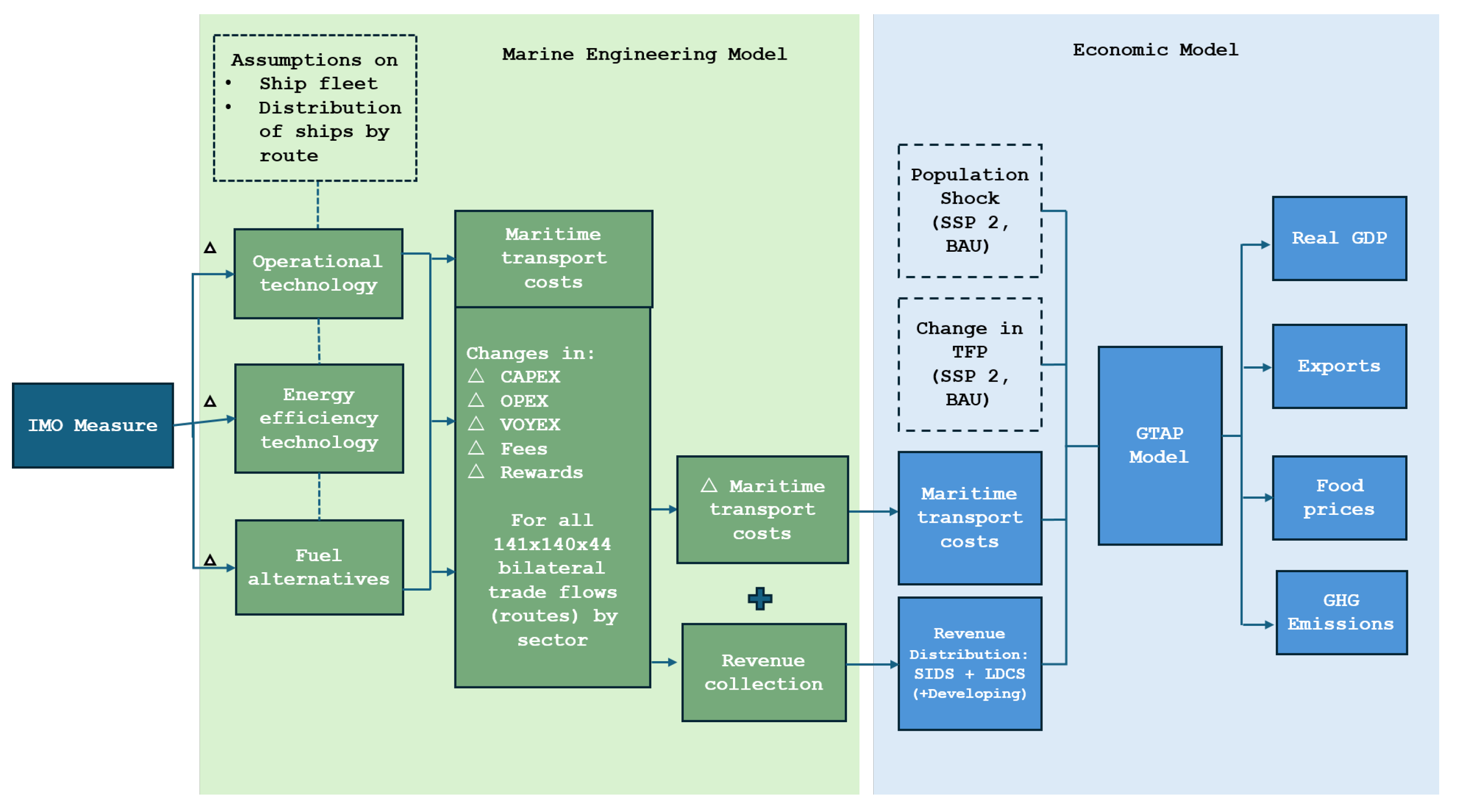
To understand the environmental and economics impacts of the policies under discussion at the IMO, the proposed methodology combines two empirical approaches. First, the Maritime Engineering Model (MEM) is used to calculate the maritime transport costs of a Business-as-Usual (BAU) scenario (or reference scenario, in which there is no climate policy) and four ‘IMO medium-term measures’ scenarios (IMO scenarios or climate policy scenarios). Each medium-term measure scenario considers an MBM currently being discussed at the IMO (described in Section 2) associated with technological alternatives to achieve the goals of the short-term measures already implemented by the shipping sector to reduce GHG emissions. In this way, what distinguishes IMO medium-term scenarios is the specific economic instrument considered in each case (e.g., levy, feebate, or remedial or surplus units, as in FCM original or FCM revised). In the MEM, we account for operational measures, energy efficiency improvements, fuel technologies, and economic instruments.

Second, the maritime transport cost difference between IMO and BAU scenarios (in percentage terms) is fed into the economic modeling as a transport cost shock. This shock accounts for the changes in the cost of international shipping to quantify the regional economic effects of the measures in the 2027–2035 period. It is worth mentioning that the simulations are performed annually from 2018 to 2035, as the base year of GTAP is 2017; however, the medium-term measures enter into force only in 2027. The designed scenarios used in the economic approach (see Section 3.2) are in line with those simulated by the MEM (see [4] for more details). Details of the empirical framework and its two methods are illustrated in Figure 1.

3.1. Marine Engineering Moddeling: Maritime Transport Cost

To calculate the maritime transport cost for different scenarios, the MEM comprises processes and input databases, breaking down the shipping system into manageable tasks to ensure robust analysis and consideration of whole-system dynamics. The model starts from a baseline year (2018) using industry data and input parameters and forecasts the global fleet’s evolution using techno-economic modeling to assess individual vessels’ competitiveness in future scenarios, considering evolving fleet energy efficiency until 2035. Algorithms simulate ship owners’ and operators’ decisions regarding fleet management and operation annually.

The MEM approach presents eight dimensions: trade, ship fleet, ship voyage, GHG policy, ship energy efficiency, fleet update, transport cost, and emissions. Ship fleet considers eight ship types, categorized by different sizes, and the size unit depends on the vessel’s service and assumes five categories of ship ages (each spanning five years); see [4] for details.

Concerning global bilateral trade flows, the MEM uses UN Comtrade data discriminated by product to calculate trade transported by sea. The same procedure as [8] (briefly presented in Section 3.2.1) was applied to derive maritime trade flows from total trade data (which include ground and air transported trade). Trade data are aggregated by country or region (141), and tradeable goods (44) using the same aggregation as the GTAP model. Trade projections from 2019–2035 are made using population and GDP forecasts from the SSP 2 scenario from IPCC. In turn, the ship fleet is categorized by assigning the appropriate ship type, size, age, speed, and energy efficiency to each trade flow/product, and ship voyages to transport annual loads for each trade flow, focusing on travel distances and shipping transport work, are simulated (The navigation distance for each trade flow is defined using a matrix from approximately 1400 port terminals, aggregated by region. The model considers load ships based on capacity and type (according to cargo loading factors defined by the 2nd IMO GHG study), calculates the number of voyages needed, and assesses travel time considering average ship speeds. Criteria for maximum travel time, especially for perishable goods, were applied). The ship fleet profile, total distance traveled, and shipping transport work are validated using external data such as AIS databases; see [4] for details.

3.2. Economic Modelling: GTAP

After calculating the change in maritime transport costs by bilateral maritime trade flow and sector, we assess the impacts on economic outcomes using the GTAP, a Computable General Equilibrium (CGE) model. GTAP enables us to simulate how the global economy would react if all regions implemented the medium-term measures under discussion at the IMO. CGE models are particularly well-suited for this type of analysis, as they indicate both the direction and magnitude of impacts while accounting for underlying uncertainties. Unlike forecasting, which involves probability and short-term predictions, CGE-based scenario simulation focuses on exploring what is possible, providing a broader understanding of potential outcomes. By combining the model with multiple scenarios, we can explore a wide range of possibilities, offering policymakers insights into potential trade-offs and unintended consequences—critical factors for informed decision-making (for more details, see https://www.gtap.agecon.purdue.edu/ accessed on 1 April 2025).

We utilize the latest version of the GTAP database (version 11, base year 2017), which contains data on 141 countries, 19 aggregated regions, and 65 sectors. These sectors include three transport margin sectors (water transport, air transport, and other transport), fuel commodities (coal, oil, gas, petroleum products, and electricity/gas manufacture distribution) and five factors of production (land, skilled labor, unskilled labor, natural resources, and capital).

For the simulations in this study, we further aggregated countries/regions into 96 regions based on economic homogeneity, i.e., similar economic structures or trade patterns, and other considerations such as geographic proximity and economic integration. This ensures that regions behave similarly in the model. Using the same principle, sectors are aggregated into 44 categories, based on similarities in production processes, factor usage, and market behavior (reducing the regional and sectoral aggregation is a common practice in CGE studies, as it ensures that the model remains both manageable and representative of real-world economic interactions). (see

Table A1. Aggregation of sectors based on the GTAP sectoral codes.

ID	GTAP Code	Description
1	pdr	Rice: seed, paddy (not husked).
2	wht	Wheat: seed, other.
3	gro	Other Grains: maize (corn), sorghum, barley, rye, oats, millets, other cereals.
4	v_f	Vegetables & Fruits: vegetables, fruit and nuts, edible roots and tubers, pulses.
5	osd	Oil Seeds: oil seeds and oleaginous fruit.
6	c_b	Sugar Crops: sugar cane and sugar beet.
7	pfb	Plant Fibers: cotton, flax, hemp, sisal, and other raw vegetable materials used in textiles.
8	ctl	Cattle: bovine animals, live, other ruminants, horses, and equines.
9	oap	Other Animal Products: swine, poultry, eggs, honey, skins, furs, and animal waxes.
10	frs	Forestry: logging and related service activities.
11	fsh	Fisheries: fishing and aquaculture.
12	coa	Coal: mining and agglomeration of hard coal, lignite, and peat.
13	oil	Oil: extraction of crude petroleum.
14	gas	Gas: extraction of natural gas.
15	oxt	Other Mining: mining of metal ores; other quarrying.
16	cmt	Cattle Meat: fresh or chilled meat of bovine, sheep, goat, and other mammals.
17	omt	Other Meat: meat of pigs, poultry, and other animals, fresh or frozen.
18	vol	Vegetable Oils: margarine, oil-cakes, and residues of vegetable oil extraction.
19	mil	Milk: dairy products.
20	sgr	Sugar and molasses.
21	ofd	Other Food: processed and preserved foods, bakery products, and animal feed.
22	b_t	Beverages & Tobacco: includes alcohol and tobacco processing.
23	tex	Textiles: manufacture of textiles.
24	wap	Wearing Apparel: clothing manufacturing.
25	lea	Leather & Related Products: processing of leather and hides.
26	lum	Lumber: wood processing and related activities.
27	ppp	Paper & Paper Products: includes printing and publishing.
28	p_c	Petroleum & Coke: refining of crude petroleum.
29	chm	Chemicals: manufacture of industrial chemicals.
30	bph	Pharmaceuticals: medicinal and botanical products.
31	rpp	Rubber & Plastic Products: manufacture of synthetic materials.
32	nmm	Non-Metallic Mineral Products: glass, ceramics, cement, etc.
33	i_s	Iron & Steel: production and basic casting.
34	nfm	Non-Ferrous Metals: aluminum, copper, zinc, gold, and silver.
35	fmp	Fabricated Metal Products: excluding machinery.
36	ele	Electronics: manufacture of computers and optical products.
37	eeq	Electrical Equipment: appliances, components, and electrical machinery.
38	ome	Machinery & Equipment: general industrial machinery.
39	mvh	Motor Vehicles & Parts: automobile manufacturing.
40	otn	Other Transport Equipment: ships, aircraft, and railway equipment.
41	omf	Other Manufacturing: includes furniture and miscellaneous industries.
42	cns	Construction: infrastructure, commercial, and residential building.
43	trd	Trade: wholesale & retail trade activities.
44	ser	Services: business, public administration, and financial services.

Notes: ‘ID’ means identification. ‘GTAP Code’ means 3-digit code used by the GTAP model.

in Appendix A).

Regarding international trade and transport margins in GTAP, trade flows from the source region to the destination region create demand for trade and transport services (the GTAP model employs the “Armington Assumption” in the trading sector, which allows one to distinguish imports by their origin and explains intra-industry trade of similar products). The GTAP model includes separate conditional demand equations for domestic and imported intermediate inputs. The sourcing of imports is done at the regional level, in the destination country. Based on a Constant Elasticity of Substitution (CES) preference function, import demand for each good by region of origin is guided by a substitution elasticity for imports by destination region. In turn, the demand for transport services is proportional to the delivered quantity, with potential transport efficiency improvements (Captured by the technical coefficient “atmfsd”. For more details on the trade and transportation market in GTAP, see [8]).

The impact of medium-term measures on GDP, trade, and prices is assessed by comparing the BAU scenario with each of the IMO scenarios in relative terms, capturing percentage changes (in percentage points). The results consider both direct and indirect effects, reflecting interactions and feedback taking place in the economic system. The scenarios utilized in the economic modeling are outlined as follows:

BAU Scenario: The BAU scenario follows the Shared Socioeconomic Pathway (SSP) 2 from the IPCC, which projects GDP and population trends that reflect a continuation of current patterns, with moderate challenges in addressing climate change and pursuing mitigation and adaptation efforts. All simulated scenarios run from 2018 to 2035, representing an economic adjustment period for GDP and population dynamics. We compute the variation in factor productivity obtained after economic adjustment and incorporate them as a new shock to model the BAU scenario. This step allows us to endogenize GDP in the climate policy shock, capturing the net effect of the IMO’s short- and medium-term measures. Consequently, changes in production, consumption, and investment under the IMO scenarios will influence GDP and other macroeconomic variables. The model adjusts dynamically to demand and supply shifts, maintaining interactions among economic agents.

IMO medium-term measures scenarios: Each IMO medium-term scenario incorporates BAU economic adjustments (GDP and population) and transport price changes resulting from the measure being analyzed, alongside short-term measures already adopted. The IMO medium-term scenarios are as follows:

(i)

Levy scenario: Maritime transport price changes resulting from the GHG levy (as described in Section 2) combined with short-term measures.

(ii)

Feebate scenario: Maritime transport price changes resulting from the proposed feebate mechanism (as described in Section 2), in combination with short-term measures.

(iii)

Original GFI flexibility mechanism scenario: Maritime transport price changes resulting from the original GFI flexibility mechanism (as described in Section 2) associated with short-term measures.

(iv)

Revised GFI flexibility mechanism scenario: Transport price changes resulting from the revised GFI flexibility mechanism (as described in Section 2) associated with short-term measures.

In addition, based on the levy revenue collection, which is derived from the simulated GHG levy scenario, we also simulate two scenarios considering revenue disbursement (as explained in Section 3.2.2): (i) Revenue disbursement scenario 1: Maritime transport price changes derived from the GHG levy, associated with the short-term measures and to the revenue disbursement to developing countries, Least Developed Countries (LDCs), and Small Island Developing States (SIDs), according to United Nations’ country list classification (https://www.un.org/ohrlls/content/list-sids accessed on 1 April 2025; https://www.un.org/ohrlls/content/list-ldcs accessed on 1 April 2025); (ii) Revenue disbursement scenario 2: Maritime transport price changes resulting from the GHG levy, combined with the short-term measures and to the revenue disbursement to Least Developed Countries (LDCs) and Small Island Developing States (SIDS), as described in the previous section.

All scenarios are implemented by changing maritime transportation cost, with each scenario varying in cost-change factors. Moreover, all scenarios also include updates on population growth and changes in total factor productivity, aligned with GDP evolution forecasts under the SSP2 scenario.

3.2.1. Modeling Maritime Transport Cost in GTAP

In this assessment, we quantify the the impact of medium-term measures under discussion at the IMO on maritime transport costs, considering their interaction with short-term measures (EEDI, EEXI, and CII) over the 2023–2035 period. Anticipated technological improvements are implicit in the IMO scenarios simulated using GTAP.

To calculate the impacts of maritime cost changes in GTAP, we have included three key elements into the model: (i) international trade shares transported by shipping; (ii) transport mode substitution elasticities; (iii) a shifter price variable, enabling exogenous adjustments in maritime transport cost for different commodities and bilateral trade routes. These three steps represent important novelties to the methodology employed in the sector and are detailed in [8].

Estimating Trade Shares Transported by Ships: To accurately estimate maritime price shocks in GTAP, we predict the share of international trade transported by sea. This is done using a LASSO (Least Absolute Shrinkage and Selection Operator) regression model, a machine-learning technique that leverages origin–destination–product characteristics and geographic controls (Such as GDP, distance, language, colonial ties, and landlocked status. This machine-learning procedure was employed as it generates better predictions (smaller prediction errors) than regular econometric methods as Lasso regression focuses on predicting the outcome variable, rather than identifying a specific effect on the outcome variable). Our approach is based on [31] (we assume that modal shares remained relatively stable from the 2000s (the [31] dataset reference years to 40 regions and 23 industries) until 2017, based on the assumption that relative freight prices by transport mode did not vary significantly during this period).

Estimating Transport Mode Substitution Elasticities: To assess potential substitution effects between transport modes due to changes in maritime shipping costs, we estimate transport mode substitution elasticities (sea–air or air–sea) based on [32] international trade and transport price data (Data set covering US imports from 1974 to 2004, with detail on exporting country x SITC revision 2 (5 digits) commodity and transport mode. It contains shipment values, weight, quantity, tariffs, and transportation charges. The substitution elasticity between sea–land transportation modes is assumed to be equal to zero due to lack of data). For products primarily transported by sea (or air), we did not consider modal substitution, such as cereal grains, vegetables and fruits, bovine cattle, coal, gas, bovine meat products, petroleum coal products, and ferrous metals, among others.

Implementing a Price Adjustment Mechanism: Once we estimate (i) international trade shares transported by ships and (ii) transport mode substitution elasticities, we integrate a price variable for each transport mode on the demand side of the GTAP model. This allows us to replace an equivalent slack variable, which can then be adjusted to simulate changes in maritime transportation costs by commodity and trade partner. The formulation of the modified maritime transport price variable is presented in Equation (1).

$$ptran{s}_{m,i,j,s}=vtfsd\_ms{h}_{m,i,j,s}·[p{t}_m-atmfs{d}_{m,i,j,s}]+shifte{r}_{m,i,j,s}$$

(1)

In which $ptran{s}_{m,i,j,s}$ is the flow-specific average costs of maritime transport; $vtfsd\_ms{h}_{m,i,j,s}$ represents the maritime share in the transport cost of commodity s from region i to j; $[p{t}_m-atmfs{d}_{m,i,j,s}]$ considers the total composite maritime transport costs (e.g., all costs incurred beyond the costs of the product itself, $p{t}_m$) adjusted for the efficiency or productivity of maritime transport along each route ($atmfs{d}_{m,i,j,s}$), which is endogenous and driven by product, source, and destination-specific determinants. This technological change can affect how commodities are transported across international borders, leading to changes in shipping costs, trade patterns, and economic outcomes in the model. Finally, the $shifte{r}_{m,i,j,s}$ variable is an exogenous price adjustment term that allows us to incorporate additional price changes beyond the endogenous cost structure. It is a calibrated parameter set to reflect specific policy-driven or external cost variations in maritime transport. Its values are based on the MEM; more details can be found in [4] regarding decarbonization pathways and cost pass-through in shipping. While a fully endogenous determination of this variable would require structural modifications to the GTAP model, its calibration is consistent with the cost and efficiency changes proposed in our engineering-based maritime transport model.

Modeling the Impact of Maritime Cost Changes: The impact of the maritime transport cost change is calculated using GTAP shipping cost data (in millions of USD), following the methodology described by [33]. The impact of cost changes is given by Equation (2):

$$\delta s_{m,i,j,s}={\displaystyle \frac{\Delta transport-cos{t}_{m,i,j,s}}{margincos{t}_{m,i,j,s}}}$$

(2)

in which ($\Delta transport-cos{t}_{m,i,j,s}$) is the change in maritime transport cost (m) for commodity s from country i to country j. The $margincost$ variable is the baseline maritime transport cost computed within GTAP.

The cost change impacts the model by changing relative transport prices (Equation (3)):

$$TransportPrice{s}_{m,i,j,s}=margincos{t}_{m,i,j,s}(1+{\Delta }_m+{\Delta }_i+{\Delta }_j+\Delta s_{m,i,j,s})$$

(3)

The calculated shock ($\delta s_{m,i,j,s}$) considers both technical and operational changes, as well as the adoption of economic instruments (medium-term measures), as explained in Section 3.2.

3.2.2. Modeling Revenue Recycling Mechanisms in GTAP

In principle, a carbon levy internalizes climate external costs by increasing the cost of goods and services per unit of carbon emitted, ideally reflecting the social cost of carbon for a given baseline. Even when globally coordinated (to preserve national competitiveness) and consistently applied (to avoid carbon leakage), recent studies show that carbon taxes have heterogenous distributional effects, disproportionally affecting low-income countries compared to high-income countries, as well as poorer groups within all countries [34,35,36]. Thus, distributing the revenue addedgenerated from carbon taxation to poorer countries (typically the most negatively affected) or those most vulnerable to climate impacts can contribute to alleviating these undesired distributional effects.

We incorporate revenue distribution in two of the simulated scenarios. We model the revenue distribution exogenously in GTAP by first calculating the global revenue generated in the levy scenario and then redistributing it as income transfers to the countries negatively affected, according to two criteria levels. The first level specifies the eligible countries as those that have experienced a negative GDP impact in the levy scenario without revenue distribution, selecting from SIDS, LDCS, and developing countries. The two revenue disbursement scenarios are as follows: (i) Revenue disbursement scenario 1—includes SIDS, LDCS, and developing countries; (ii) Revenue disbursement scenario 2— includes only SIDS and LDCS.

In the second level, the amount of revenue allocated to each beneficiary country is proportionally to the GDP impact multiplied by the country’s/region’s population size, as illustrated in Equation (4) (we use a similar approach as discussed at the IMO, whose final document can be assessed from the technical report from [37]):

$$re{v}_i={\displaystyle \frac{y_i{p}_i}{{\sum }_{j=1}^n{y}_j{p}_j}}R$$

(4)

where R is the total revenue to be disbursed, $y_i$ is the percentage impact on the GDP of country i, $p_i$ is the population size of country i, and j is the index of the beneficiaries’ countries included in the sum.

To implement the revenue disbursement scenarios in GTAP, we use the income slack variable, which allows for flexibility in income adjustments and analysis of the distributional effects of policies. It is worth noting that revenue distribution was simulated as an income transfer to the beneficiaries’ economies as a whole. Increasing the complexity of revenue allocation would require incorporating additional equations to model specific mechanisms, such as reinvesting revenues within the maritime sector, R&D activities, or incentivizing fuel efficiency improvements. However, besides not being sector-specific, the revenue disbursement scenarios contributes to the overall analysis of the economic impacts of adopting a levy.

4. Descriptive Statistics: Maritime Transport Cost—MEM vs. GTAP

In this section, we validate our data by comparing maritime transport cost data from GTAP with those calculated by the MEM.

Table 2. Comparison between maritime transport cost data in the BAU scenario, GTAP, and OEM.

Year	Maritime Cost (GTAP): “wtp” Variable, in Billion Dollars	Maritime Cost (OEM): CAPEX and OPEX Total Costs, in Billion Dollars	Difference (%)
2023	327.55	321.73	1.8%
2024	328.12	322.21	1.8%
2025	328.74	322.89	1.8%
2026	329.34	323.69	1.7%
2027	329.99	324.66	1.6%
2028	330.67	325.95	1.4%
2029	331.40	327.41	1.2%
2030	332.16	329.27	0.9%
2031	332.82	331.47	0.4%
2032	333.52	334.15	−0.2%
2033	334.25	337.53	−1.0%
2034	335.01	342.10	−2.1%
2035	335.80	345.75	−2.9%

presents both datasets for the 2023–2035 BAU scenario, which assumes the regular evolution of costs based on transport demand growth, without considering any medium-term measures. The results show that the differences between the two datasets are relatively small, ranging from −2.9% to 1.8%, indicating a high degree of comparability between the estimates.

For the sectoral effect, we find that the GHG levy leads to a greater cumulative increase in transport costs (

Table 3. Increase in maritime transport costs, in %, compared to the reference scenario (BAU), by sector in 2035.

Sector	GHG Levy	Feebate	FCM Revised	FCM Original
Beverages and tobacco products	57.9%	31.7%	21.7%	30.7%
Basic pharmaceutical products	52.0%	25.5%	16.7%	25.3%
Sugar cane, sugar beet	41.1%	25.2%	18.5%	20.8%
Chemical products	53.0%	27.0%	17.8%	26.6%
Bovine meat products	59.4%	30.9%	22.6%	28.2%
Coal	46.0%	26.1%	20.6%	21.4%
Bovine cattle, sheep, and goats	17.7%	22.6%	10.2%	9.8%
Computer, electronic, and optic	52.0%	26.0%	17.0%	25.5%
Metal products	41.6%	22.5%	19.3%	21.8%
Forestry	40.3%	24.3%	21.7%	21.4%
Cereal grains nec	62.4%	44.0%	36.9%	39.1%
Ferrous metals	42.1%	24.3%	18.6%	21.5%
Wood products	53.6%	26.5%	18.3%	24.8%
Dairy products	57.7%	31.3%	22.3%	29.0%
Motor vehicles and parts	51.4%	25.2%	16.4%	24.5%
Mineral products nec	52.8%	27.5%	18.2%	27.2%
Animal products nec	57.4%	30.8%	21.5%	29.2%
Food products nec	58.3%	31.9%	22.2%	31.1%
Oil and gas	54.9%	34.8%	26.0%	30.6%
Machinery and equipment nec	52.1%	25.9%	16.9%	25.3%
Manufactures nec	51.5%	25.2%	16.4%	24.8%
Meat products nec	54.7%	27.9%	19.2%	27.5%
Oil seeds	49.3%	30.6%	28.5%	30.5%
Transport equipment nec	37.3%	22.1%	20.3%	21.0%
Minerals nec	45.2%	25.5%	20.8%	21.1%
Petroleum, coal products	40.3%	27.4%	18.3%	22.4%
Rice	77.6%	56.9%	42.1%	54.1%
Plant-based fibers	59.0%	32.0%	22.8%	30.8%
Paper products, publishing	52.9%	25.8%	17.2%	25.1%
Rubber and plastic products	51.7%	25.8%	16.9%	25.3%
Sugar	49.1%	30.6%	24.5%	27.5%
Textiles	57.4%	32.0%	22.0%	31.2%
Vegetables, fruit, nuts	74.7%	50.6%	37.3%	48.3%
Vegetable oils and fats	52.2%	33.7%	31.2%	32.7%
Wearing apparel and leather	57.2%	31.5%	21.6%	30.9%
Wheat	55.4%	43.1%	35.8%	34.1%

). Certain sectors are particularly affected, including rice (77.6%), vegetables and fruits (74.7%), and cereals (62.4%). The Revised FCM results in smaller cost increases; however, the most impacted sectors remain rice (42.1%), vegetables and fruits (37.3%), and cereals (36.9%).

Table 4. Increase in maritime transport costs, in %, compared to the reference scenario (BAU), by year, 2024–2035.

Year	Feebate	GHG Levy	FCM Revised	FCM Original
2024	3.8%	3.8%	3.7%	3.8%
2025	6.0%	6.0%	5.9%	6.0%
2026	7.9%	7.9%	7.8%	7.9%
2027	14.0%	31.2%	9.8%	10.8%
2028	15.3%	31.9%	11.2%	11.4%
2029	16.5%	32.5%	12.8%	12.4%
2030	22.9%	41.9%	14.2%	14.4%
2031	23.4%	41.4%	15.8%	16.2%
2032	23.3%	41.3%	16.9%	18.0%
2033	23.5%	41.5%	18.3%	20.0%
2034	25.0%	41.9%	20.2%	22.1%
2035	29.4%	49.7%	22.2%	26.0%

presents the average annual percentage change in maritime costs, comparing the BAU scenario with the IMO medium-term measures. The results highlight significant variability in cost impacts across years, ranging from a 22.2% increase under the FCM Revised to a 49.7% increase under the GHG levy by 2035.

5. Results

In this section, we present the comparison between the BAU scenario and the IMO medium-term measures scenarios, from 2027 to 2035. In this way, the impacts on real exports, real GDP, and global price index are measured, in each of the IMO scenarios, as percentage point changes relative to the BAU scenario. All scenarios consider the evolution of trade and demand for maritime transport. Section 5.1, Section 5.2 and Section 5.3 present the results concerning the medium-term measures impacts, and Section 5.4 presents the results for the levy scenario considering two different options for revenue disbursement, as presented in Section 3.2.2. All the results also include the effects of the short-term measures.

5.1. Impacts on Real GDP

The calculated impacts on real GDP accounts for the quantity effects of the maritime costs’ variation, not accounting for potential price changes. All the IMO medium-term measures analyzed present negative impacts on real GDP between 2027 and 2035 (Figure 2). The levy scenario presents the most severe impacts, with the distribution of the losses very uneven across countries. On the other hand, the revised GFI flexibility scenario presents the mildest negative effects, followed by the original GFI flexibility mechanism and feebate scenarios. By 2035, the impact on real GDP is −0.037 p.p. (levy scenario), −0.021 p.p. (feebate scenario), −0.019 p.p. (original GFI scenario), and −0.015 p.p. (revised GFI scenario)).

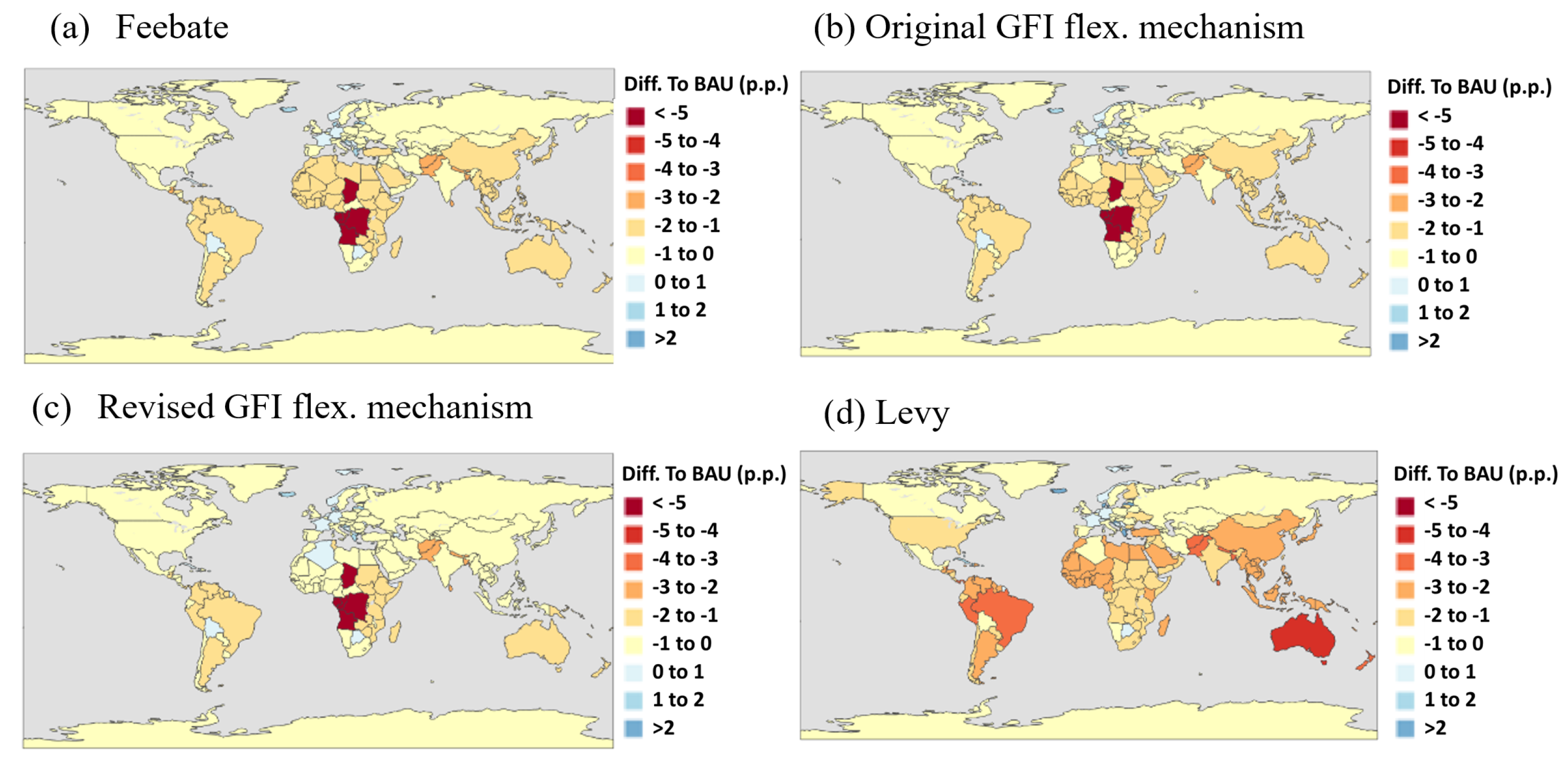
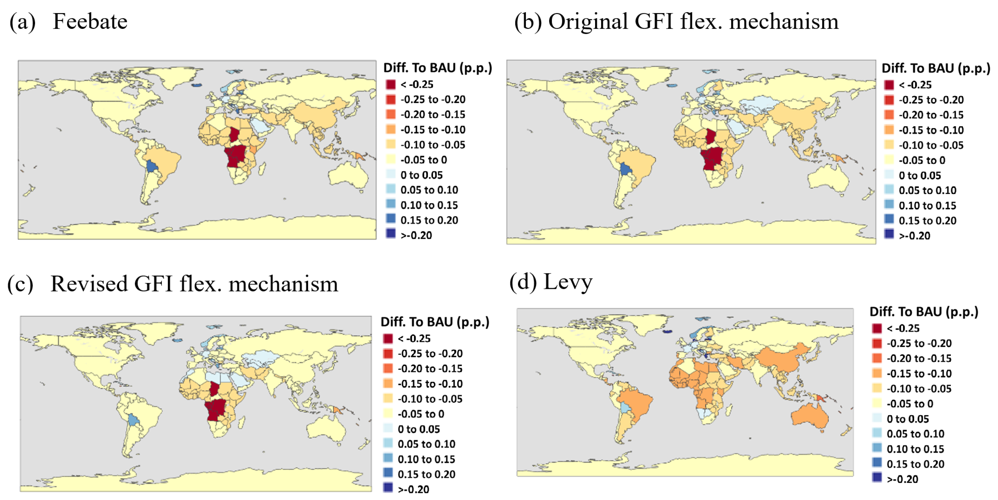
We then examine the impact of GDP variations across different countries and regions. Figure 3 illustrates the spatial distribution of these effects. The results show significant regional differences. In all IMO scenarios, the most negatively affected regions include African countries, particularly those in south-central Africa. In contrast, in all IMO scenarios, some European countries experience positive effects on GDP.

Comparing the four IMO measures, the levy scenario adds to the regions negatively affected and includes countries from western and southeast Asia, western and north Africa, Oceania, and South America to the list of the most negatively affected ones. In turn, the revised GFI flexibility mechanism attenuates the negative impacts in all regions (except to some south-central African countries).

5.2. Impacts on Trade: Real Exports

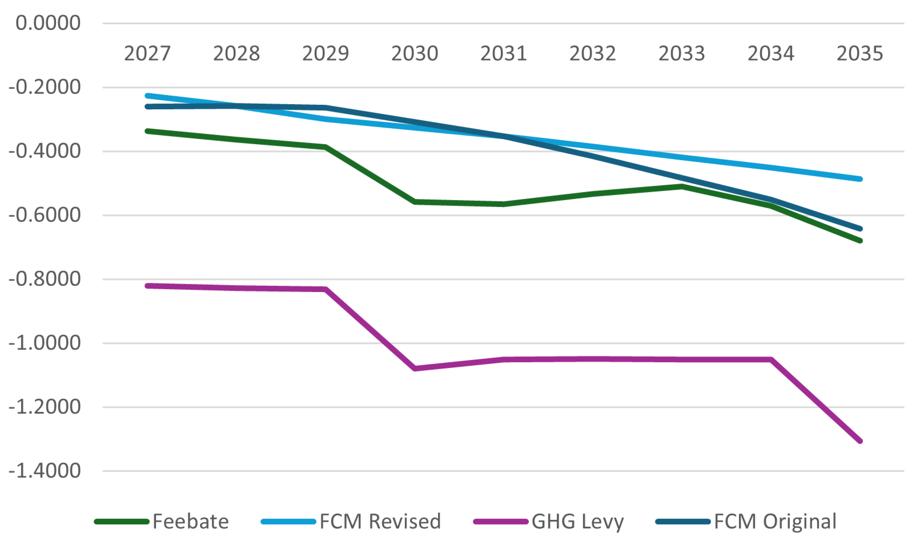
As well as GDP, real exports decrease over time in all IMO simulated scenarios, the GHG levy being the worst case and the revised GFI mechanism the best case scenarios (Figure 4). However, the magnitude of the negative impact on real exports and real imports (for more details, see Figure A1 in Appendix A) is more severe than the negative impacts on real GDP. By 2035, global exports are expected to decrease by between −1.307 p.p., under the levy scenario, and −0.487 p.p., under the revised GFI mechanism. This represents a reduction in exports of approximately USD 339 billion in the levy scenario and USD 130 billion in the revised GFI scenario, both in 2017 dollars.

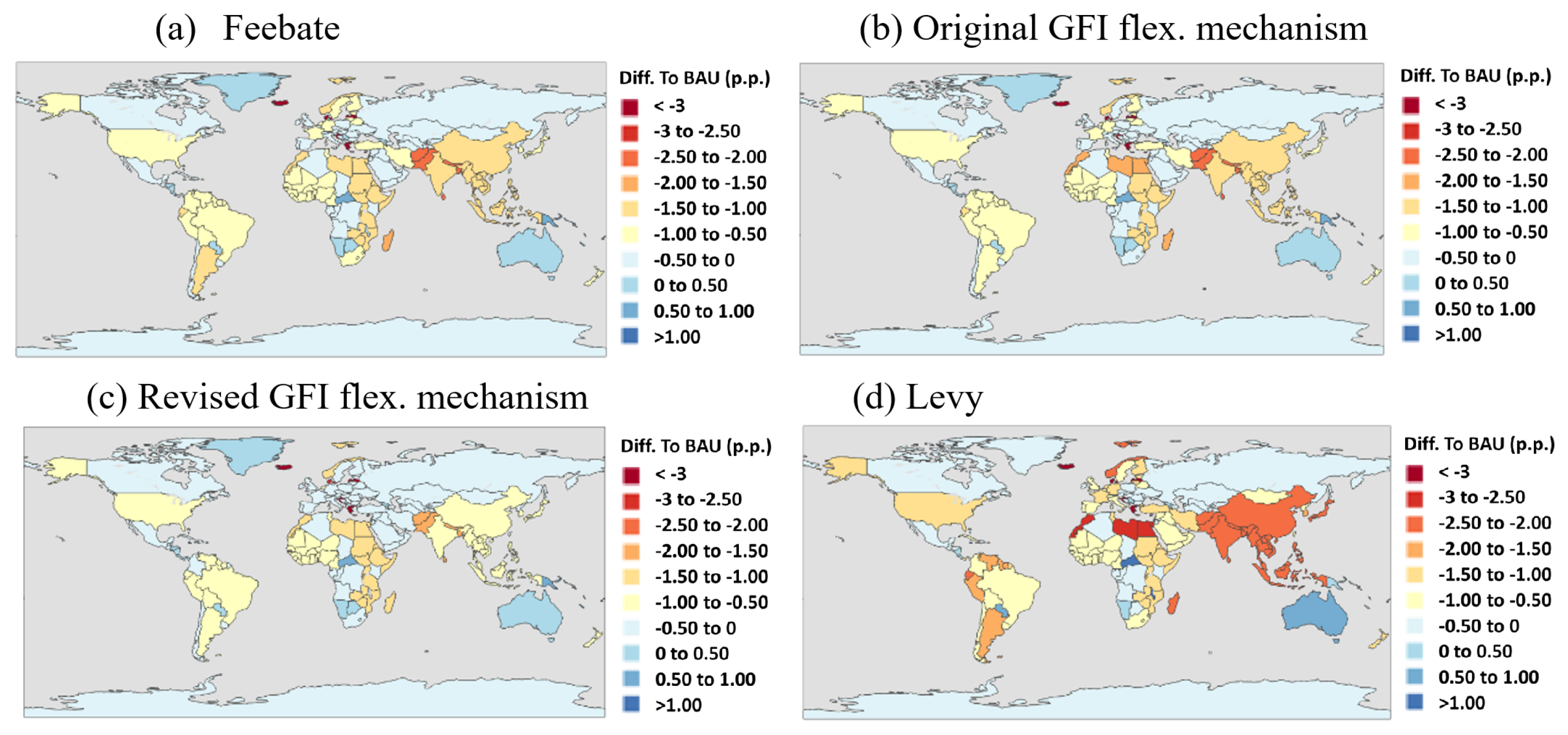
Analyzing the spatial distribution of the impacts, as shown by Figure A2 in Appendix A, the GHG levy scenario presents the greater negative impacts, especially on the countries located in south and southeast Asia, north Africa, and South America. On the other hand, the revised GFI flexibility mechanism is the scenario that presents the less pronounced negative impacts across all regions.

5.3. Impacts on Global Price Index

Table 5. Global price index change by IMO scenario and sector in 2035 (in p.p.).

Sector	Feebate	FCM Original	FCM Revised	GHG Levy
Air transport	0.298	0.264	0.214	0.505
Beverages and tobacco products	0.285	0.272	0.208	0.598
Basic pharmaceutical products	0.161	0.146	0.121	0.341
Sugar cane, sugar beet	−0.054	−0.058	−0.043	−0.034
Chemical products	0.484	0.454	0.343	1.043
Bovine meat products	0.134	0.123	0.097	0.191
Construction	0.108	0.097	0.080	0.222
Coal	0.599	0.492	0.466	1.351
Bovine cattle, sheep, and goats	0.068	0.068	0.051	0.119
Computer, electronic, and optic	0.236	0.219	0.170	0.529
Metal products	0.296	0.267	0.232	0.662
Forestry	0.051	0.036	0.038	0.261
Fishing	−0.025	−0.025	−0.008	0.152
Cereal grains nec	0.542	0.487	0.431	1.773
Ferrous metals	0.442	0.336	0.343	0.943
Wood products	0.350	0.310	0.249	0.730
Dairy products	0.188	0.180	0.137	0.337
Motor vehicles and parts	0.308	0.286	0.218	0.633
Mineral products nec	0.298	0.272	0.211	0.613
Animal products nec	0.110	0.101	0.081	0.182
Food products nec	0.330	0.314	0.249	0.526
Oil and Gas	0.657	0.596	0.509	1.009
Machinery and equipment nec	0.287	0.266	0.205	0.584
Manufatures nec	0.308	0.291	0.214	0.619
Meat products nec	0.194	0.181	0.142	0.330
Oil seeds	0.572	0.560	0.518	1.052
Transport equipments nec	0.230	0.211	0.183	0.504
Transport nec	0.137	0.122	0.101	0.237
Minerals nec	0.510	0.433	0.378	0.987
Petroleum, coal products	0.778	0.681	0.574	1.287
Rice	0.074	0.075	0.070	0.083
Plant-based fibers	0.241	0.242	0.170	0.384
Paper products, publishing	0.347	0.329	0.242	0.633
Rubber and plastic products	0.398	0.377	0.278	0.753
Accommodation, Food and services	0.078	0.074	0.053	0.137
Sugar	0.347	0.309	0.272	0.464
Electricity, distribution	0.187	0.166	0.146	0.336
Textiles	0.356	0.343	0.259	0.517
Trade	0.060	0.055	0.044	0.112
Vegetables, fruit, nuts	0.288	0.254	0.205	0.300
Vegetables oils and fats	0.565	0.539	0.522	0.715
Wearing apparel and leather	0.430	0.419	0.312	0.485
Wheat	0.505	0.447	0.430	0.433
Water transport	0.174	0.147	0.127	0.310

Notes: This table compares the global price index after accounting for population changes over time (based on SSP2) and changes in total factor productivity (aligned with GDP growth from SSP2) across all scenarios. The change in transport costs is applied exclusively to the IMO scenarios.

presents the impact on the global price index by sector in 2035, to all IMO medium-term scenarios. The average increase in the global price index is 0.29 p.p., 0.27 p.p., 0.22 p.p., and 0.52 p.p. in the feebate, GFI original, GFI revised, and levy scenarios, respectively. The levy scenario registers the highest increase in prices (two times or more than the other scenarios) of all sectors. The sectors that registered the highest increase in prices are coal (1.35 p.p.), petroleum and coal products (1.29 p.p.), oil seeds (1.05 p.p.), chemical products (1.04 p.p.), and oil and gas (1.01 p.p.). In the two scenarios that consider revenue disbursement, the increase in prices is even greater. In all IMO scenarios, except for the two scenarios with revenue distribution, only the sugar cane (−0.03 p.p.) and fishing (−0.03 p.p.) sectors showed a decrease in prices. Importantly, food prices also register an increase in all IMO scenarios of 0.33 p.p., 0.31 p.p., 0.25 p.p., 0.53 p.p., 0.57 p.p., and 0.46 p.p. in the feebate, GFI original, GFI revised, levy, levy disbursment_1, and levy disbursment_2 scenarios, respectively.

5.4. Revenue Disbursement

In this section, we present the results considering the disbursement of the revenue collected under the levy scenario, focusing on the impacts on real GDP. As described in Section 3.2, revenue allocation is simplified by distributing it to the economies as a whole, not being sector-specific. We propose two different groupings to distribute the revenue among the countries, from 2028 on (1) developing countries, SIDs, and LDCs negatively affected and on (2) only to SIDs and LDCs negatively affected.

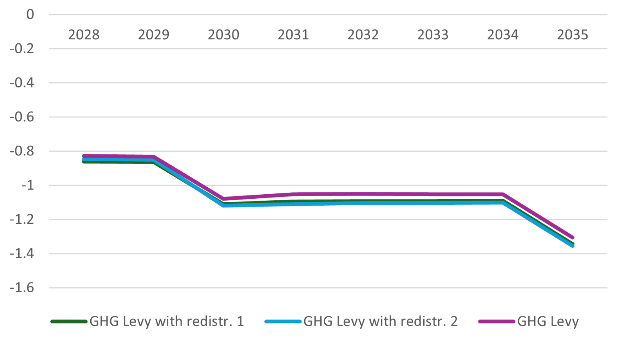
The overall effect of revenue recycling is to worsen the negative impacts on both real GDP (Figure 5) and real exports (Figure A3 in Appendix A) over the entire period.

Considering the impact on GDP, in 2030 the impact of the levy scenario without revenue disbursement was −0.032 p.p., and after revenue distribution the impact was −0.033 p.p. in revenue disbursement criteria 1 and −0.035 p.p. in criteria 2. In turn, 2035 showed a negative impact of −0.037 p.p. before revenue disbursement and −0.039 p.p. and −0.040 p.p. after revenue distribution under criteria 1 and 2, respectively.

When it comes to the effects on real exports, it was −1.08 p.p. and −1.31 p.p. in the levy scenario without revenue disbursement, in 2030 and 2035, respectively. After distributing revenue, the impacts became more negative, registering −1.11 p.p. in 2030 and −1.34 p.p. in 2035 under disbursement criterion (1) and −1.12 p.p. in 2030 and −1.35 p.p. in 2035 under disbursement criterion (2).

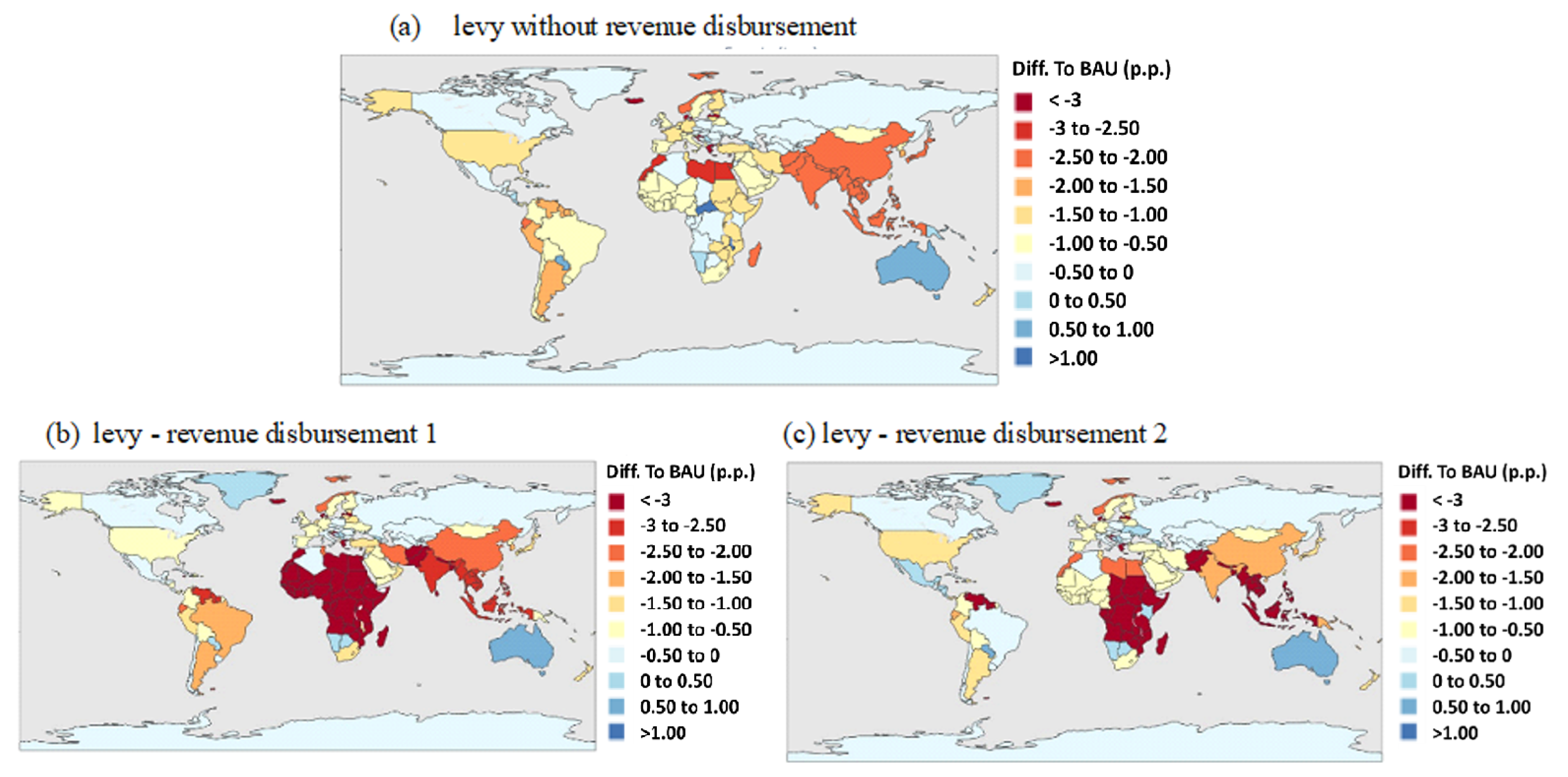
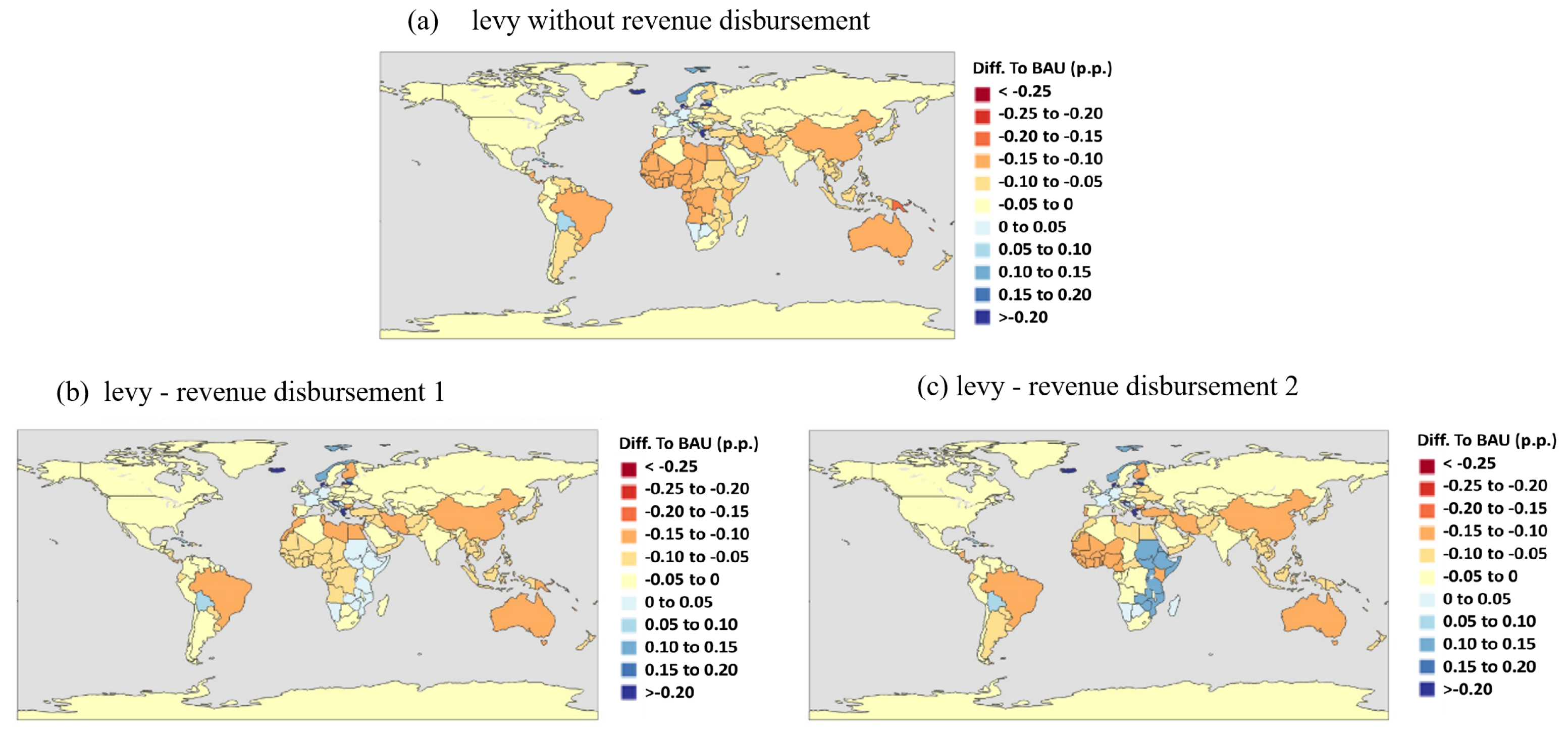
Considering the spatial heterogeneity of the effects on real GDP, the revenue distribution benefits countries of the African continent, especially in the east Africa region, with a more pronounced effect when considering revenue disbursement criterion 2 (Figure 6, panel c). Regarding real exports, the spatial effect of revenue disbursement (Figure A4 in Appendix A) is to accentuate the negative impact in countries located in the African continent (panels b and c), South America region (panel b), and south and southeast Asia regions (panels b and c). On the other hand, countries located in North America were positively impacted by revenue distribution (panels b and c).

Therefore, the revenue disbursement schemes simulated in this study do not mitigate the levy’s overall adverse effects. On the contrary, the overall effect of revenue distribution is to accentuate the levy’s negative impacts on real GDP and real exports. On average, the redistribution does not help to reduce the direct burdens of increased shipping costs or their indirect effects across sectors and international trade. Despite our simulations only considering revenue transfer in a simple way, directing it to SIDs, LDCs, and developing countries’ entire economies, they do allow one to understand the overall direction of the proposed redistribution.

5.5. GHG Emissions

Figure 7 presents the impact of the IMO medium-term scenarios on Tank-to-Wake (TTW) emissions. Our analysis shows that all measures enable the achievement of the IMO’s intermediate emission targets by 2035. Compared to the BAU scenario, emissions are projected to decrease from 535 million tons (under the revised GFI) to 607 million tons of CO₂eq (under the GHG levy) by 2035. This translates into a reduction from 52.2% to 59.3% compared to the BAU scenario. Appendix B explains how emissions were calculated.

6. Discussion

Our findings highlight the challenge of balancing environmental objectives with economic and equity considerations in designing and implementing medium-term measures to reduce GHG emissions in the maritime sector. While all measures analyzed have the potential to achieve the 2035 intermediate emissions reduction targets—surpassing 40–50% absolute reductions—their economic impacts vary significantly across regions. This heterogeneity raises equity concerns, particularly for most African and Asian countries, which experience severe economic losses in terms of GDP and trade. These findings align with prior literature emphasizing the disproportionate burdens of climate policies on developing regions, often exacerbating existing inequalities [17,38].

Among the measures analyzed, the GHG levy imposes the most substantial global economic costs, particularly affecting GDP, exports, and food prices. This is consistent with existing research on the regressive nature of carbon taxes, which disproportionately affect lower-income households and developing economies reliant on carbon-intensive goods [39,40].

Revenue distribution (revenue allocation is modeled as income transfers to the entire beneficiaries’ economies, not being sector-specific) mitigates the overall impacts on GDP and trade, generating only modest gains for African countries, suggesting that redistribution mechanisms require further refinement to mitigate adverse economic effects and address geographic disparities.

This study contributes to ongoing IMO discussions by providing a comprehensive assessment of both the environmental and economic implications of medium-term measures. Unlike much of the existing literature, which focuses on carbon taxation in specific countries or regions [12,13,15], we employ a global general equilibrium approach using the GTAP model. This methodology enables a more nuanced analysis of indirect impacts and price adjustments following policy implementation, advancing the literature on general equilibrium modeling in climate policy analysis [9]. Furthermore, we extend GTAP’s capabilities by incorporating methodologies that account for transport mode substitution and shifts in maritime transport costs, addressing the key limitations of traditional modeling frameworks [10,11].

Another contribution to the literature lies in the integration of an engineering model with a general equilibrium model to assess climate policies in the maritime sector. Most previous studies analyze operational and economic impacts separately, limiting the assessment of their interdependencies.

Our findings also underscore the importance of considering short-term costs alongside long-term outcomes. While policies such as the GHG levy are effective for long-term emissions reductions, they impose significant short-term economic burdens on regions distant from major markets and those with slower fleet transitions. These challenges reinforce the need for policy designs that balance both temporal and spatial equity. As previous studies emphasize, carbon levy mechanisms must carefully navigate the trade-offs between emissions reduction, revenue redistribution, and unintended socioeconomic consequences [36,41].

7. Final Remarks

Maritime transport is a major contributor to global GHG emissions. To decarbonize the sector, several policy measures are under discussion to achieve net-zero emissions by 2050. In this study, we assess the economic, social, and environmental impacts of IMO’s medium-term measures using a computational simulation model integrating ocean engineering and economics techniques.

Our findings suggest that all simulated medium-term scenarios have the potential to achieve the IMO’s intermediate GHG emission targets by 2035, with absolute reductions exceeding 50%. Our study reiterates that equity considerations are central to climate policy. While revenue redistribution can mitigate some regressive effects of carbon levies, the optimal allocation of revenues has no consensus among researchers or policymakers. Transfers to low income economies or in-sector, such as subsidized clean energy transition, investment in R&D, or public transportation, are alternative options. Also, the eligible countries can be defined according to their vulnerability to climate change effects, which can be combined to income aspects. Additionally, it also introduces complexities and potential rebound effects that could undermine emissions reduction efforts. Policymakers must integrate flexible, context-sensitive mechanisms that prioritize equity without compromising environmental goals.

While this study focuses on the IMO’s global measures, we acknowledge that regional policies—such as the EU’s efforts to include maritime transport in the EU ETS—are imposing stricter requirements on a subset of global shipping routes. These regional measures may create regulatory asymmetries and spillover effects that interact with global policies, potentially shaping their effectiveness and competitiveness. Although a detailed analysis of these interactions is beyond the scope of this study, future research could explore how the synergy between regional and global policies influences maritime decarbonization and trade dynamics (To address this, we incorporate key macroeconomic projections—such as population growth and total factor productivity—based on the Shared Socioeconomic Pathway 2 (SSP2) scenario. Our results compare a Business-as-Usual (BAU) scenario with various policy interventions, allowing for a structured assessment of potential trade-offs and unintended consequences, thereby supporting informed decision-making).

Finally, we acknowledge three limitations that emerged from the study. First, future projections inherently carry some degree of uncertainty, especially over longer time horizons (To address this, we incorporate key macroeconomic projections—such as population growth and total factor productivity—based on the Shared Socioeconomic Pathway 2 (SSP2) scenario. Our results compare a Business-as-Usual (BAU) scenario with various policy interventions, allowing for a structured assessment of potential trade-offs and unintended consequences, thereby supporting informed decision-making). Therefore, the scenarios should be interpreted as plausible futures rather than definitive forecasts. Second, country aggregation is based on data availability, which may not fully reflect the economic characteristics of individual nations. Data limitations pose a challenge for any analytical approach and are mostly relevant for SIDS and LDCs, which are often grouped into broader regional categories due to insufficient country-specific data.

Additionally, maritime transport costs in GTAP rely on estimated modal shares, leading to inconsistencies in transport cost data, especially for economies with limited trade data availability. Third, in our GHG levy scenario, revenue redistribution is modeled as a general allocation to eligible economies, without considering sector-specific disbursement. This simplification may overlook sectoral dynamics and their influence on broader economic outcomes. While increasing the complexity of revenue allocation in the modeling is beyond the scope of the current study, we highlight it as a key avenue for future research on the topic.

Despite these limitations, by employing a general equilibrium framework, this study provides a comprehensive assessment of the economic and distributional effects of MBMs, helping to inform policy discussions at the IMO. The results highlight trade-offs between emissions reductions and the economic impacts of different proposals, emphasizing the need for equity considerations in policy design.