Abstract
Maritime transport accounts for approximately 3% of global greenhouse gas (GHG) emissions, a figure projected to rise by 17% by 2050 without effective mitigation measures. Achieving zero-emission shipping requires a comprehensive strategy that integrates regulatory frameworks, alternative fuels, and energy-saving technologies. However, existing studies often fail to provide an integrated analysis of regulatory constraints, economic incentives, and technological feasibility. This study bridges this gap by developing an integrated model tailored for international maritime transport, incorporating regulatory constraints, economic incentives, and technological feasibility into a unified framework. The model is developed using a predictive approach to assess decarbonization pathways for global shipping from 2018 to 2035. A multi-criterion decision analysis (MCDA) framework, coupled with techno-economic modeling, evaluates the cost-effectiveness, technology readiness, and adoption potential of alternative fuels, operational strategies, and market-based measures. The results indicate that technical and operational measures alone can reduce emissions by up to 44%, while market-based measures improve the diversity of sustainable fuel adoption. Biofuels, particularly BISVO and BIFAME, emerge as preferred alternatives due to cost-effectiveness, while green hydrogen, ammonia, and biomethanol remain unviable without additional policy support. A strict carbon levy increases transport costs by 46%, whereas flexible compliance mechanisms limit cost increases to 14–25%. The proposed approach provides a robust decision-support framework for policymakers and industry stakeholders, ensuring transparency in evaluating the trade-offs between emissions reductions and economic feasibility, thereby guiding future regulatory strategies.
1. Introduction
Maritime transport is a vital backbone of global trade, yet it contributes roughly 3% of global greenhouse gas (GHG) emissions—a share comparable to industrialized nations like Germany or Japan [1,2]. Without effective mitigation, shipping emissions are projected to rise by about 17% by 2050 [3], posing a serious challenge to international climate goals. Recognizing this, the International Maritime Organization (IMO) has introduced ambitious targets, including a strategy to halve shipping GHG emissions by 2050 (from 2008 levels) and a 2023 revised goal aiming for net-zero emissions in the sector by 2050 [4]. Achieving these targets requires a comprehensive decarbonization strategy encompassing energy efficiency technologies, alternative low-carbon fuels, and market-based measures like carbon pricing [5,6,7]. Consequently, decarbonizing the shipping industry has become an essential component of global climate-mitigation efforts, demanding integrated solutions that align technological innovation with economic and regulatory realities.
In pursuit of these goals, IMO has proposed various measures to accelerate decarbonization in the sector and reduce GHG emissions from ships [8]. Among these efforts, IMO introduced initial measures such as the Energy Efficiency Design Index (EEDI) [9] and the Ship Energy Efficiency Management Plan (SEEMP) [10], conceived to enhance the energy efficiency of vessels built after 2012. More recently, short-term measures such as the Energy Efficiency Existing Ship Index (EEXI) [11] and the Carbon Intensity Indicator (CII) [12] have been implemented. Since November 2022, these measures mandate ships to monitor and improve their energy efficiency to avoid penalties. These initiatives have spurred significant investments in advanced technologies and infrastructure, including cleaner engines, hybrid propulsion systems, optimized hull designs, and more efficient navigation practices. However, while these changes are necessary, they have also increased operational and capital costs, underscoring the importance of international collaboration to ensure their effective implementation and compliance.
Following the 2023 revision of emission targets, attention has shifted to medium-term measures, which are essential for achieving the net-zero goal. These include regulatory frameworks and economic incentives to support decarbonization, such as a GHG levy, flexible compliance mechanisms based on GHG Fuel Intensity (GFI), and feebate systems. These tools aim to drive further emission reductions across the maritime sector. Yet, predicting the technological pathways the industry will adopt remains challenging due to the diversity of vessel types, sizes, ages, and operational profiles—each subject to varying regulatory pressures, fluctuating fuel prices, and rapid technological advancements.
Despite broad agreement on the need for deep cuts in maritime emissions, existing studies often address isolated pieces of the puzzle rather than the whole picture. Prior research has typically focused on individual decarbonization measures—for example, exploring alternative fuels (biofuels, hydrogen, ammonia) [13,14,15,16], evaluating specific energy efficiency improvements [17,18], or examining policy instruments like emission regulations and market-based measures [17,18,19]. Other works have developed global fleet emission models, but these often emphasize one dimension at a time (such as operational changes, a particular alternative fuel, or a carbon levy). What is largely missing is an integrated framework that captures the interaction between technological options, economic factors, and policy constraints. Even advanced Integrated Assessment Models (IAMs) have historically treated international shipping in a cursory manner—typically as a single aggregated sector—thereby overlooking the rich heterogeneity of vessel types and operational decisions [20]. This segmented approach in the literature means we have a limited understanding of how different strategies combine in practice, and how ship owners might navigate complex trade-offs under real-world conditions. In short, a gap exists in current GHG-assessment methods for shipping: no existing study fully integrates regulatory drivers, economic incentives, and technological feasibility into a unified, vessel-level analysis.
Integrated Assessment Models (IAMs) have long served as essential tools for evaluating global climate-mitigation strategies by linking economic systems, technological developments, and policy interventions. However, maritime transport has traditionally received limited attention within these models, despite contributing around 0.7 GtCO2 annually—or approximately 2.8% of global CO2 emissions [20]. In response, recent efforts have been made to enhance the representation of international shipping within IAM frameworks.
For instance, a comparative analysis involving six prominent IAMs—COFFEE, IMAGE, PROMETHEUS, TIAM-UCL, IMACLIM-R, and WITCH—suggests that shipping emissions could be reduced by up to 86% by 2050, primarily through the adoption of low-carbon fuels such as biofuels, renewable alcohols, and green ammonia [20]. Notably, models like COFFEE, IMAGE, and TIAM-UCL offer greater technological granularity by including multiple propulsion systems and fuel pathways, while IMACLIM-R and WITCH focus on a narrower subset of mitigation strategies. These differences highlight the variation in the predictive capacity of IAMs for the maritime sector and underscore the need for higher-resolution modeling.
Nonetheless, IAMs still rely on macroeconomic, sector-wide assumptions, often overlooking ship-specific operational and technological decisions. To address this gap, our approach integrates a sectorial simulation framework with a ship-level techno-economic model using Multi-Criteria Decision Analysis (MCDA). This allows for a more granular evaluation of decarbonization pathways tailored to different vessel types, propulsion technologies, and operational scenarios, supporting realistic and actionable strategies for achieving net-zero emissions.
Literature studies often lack an integrated framework that accounts for the interaction between regulatory pressures, volatility in fuel prices, and specific characteristics of vessels. Furthermore, there appears to be a trend in examining the problem from an economic or environmental perspective, not adequately addressing the broader complexity of deciding which technologies to adopt for different vessel types and operational contexts. Consequently, there is limited understanding of how shipowners navigate uncertainty when faced with multiple factors, including economic incentives, regulatory requirements, and technological feasibility. This paper aims to bridge this gap by developing a predictive model that integrates these aspects, offering information on the likely decarbonization paths for the maritime sector.
The maritime industry is characterized by a wide variety of vessels, from small coastal ships to large transoceanic container vessels, each with unique energy requirements and operational patterns. The introduction of new regulations, such as emission limits and carbon pricing, adds complexity to this environment, requiring shipowners to make decisions under conditions of significant uncertainty. Understanding which technologies will be adopted and how vessel classes will evolve under these changing conditions remains a critical research question. The dynamic interplay between regulatory frameworks, economic incentives, and the availability of alternative fuels further complicates predictions of the sector’s decarbonization pathways. Addressing these uncertainties is essential for developing effective policies and investment strategies to guide the maritime industry toward its decarbonization objectives.
Given this context, the primary objective of this paper is to develop a comprehensive framework to predict the decarbonization pathways of maritime transportation. This framework enables a detailed assessment of transport costs, including capital expenditures (CAPEX), operational expenditures (OPEX) and voyage-related expenditures (VOYEX), fees, and rewards, as well as the emissions associated with the adoption of new technologies over time. By providing these insights, this study seeks to facilitate the evaluation of various decarbonization policies currently under discussion at the IMO.
Building on this integrated framework, our study makes several unique contributions to the literature and practice of sustainable shipping. First, we develop a unified model that merges ship-level decision analytics with sector-wide simulation—offering a holistic perspective that fills a crucial methodological gap in maritime decarbonization research. Second, our model captures the distinct pathways for various segments of the fleet—from small coastal ships to large ocean-going vessels—showing how each segment may optimally combine technologies to meet emissions targets. Third, the integration of detailed cost assessments (CAPEX, OPEX, voyage expenses, carbon fees or credits) with emissions performance delivers a rigorous techno-economic analysis. Lastly, the framework acts as a virtual policy laboratory, revealing how specific policy measures (e.g., carbon levies, fuel intensity standards) influence technology uptake and emissions trajectories across the global fleet. Through these innovations, the study not only addresses a critical research gap but also pushes the envelope of methodological practice in maritime environmental analysis.
The specific research questions addressed in this paper are as follows:
- What are the most likely technological pathways the different ship types will adopt to comply with decarbonization regulations?
- How do fluctuating fuel prices and new regulatory measures influence the adoption of low-carbon technologies by vessels of varying types, sizes, and operational profiles?
- What are the expected costs, including CAPEX, OPEX, VOYEX, fees, and rewards, associated with the implementation of decarbonization measures?
The remainder of this paper is organized as follows. Section 2 outlines the methodology adopted and the development of the technological pathway model, including the description of the method for ranking technological options. Section 3 presents the results and discussion, encompassing cost analyses, GHG emissions evaluation, the cost-effectiveness of decarbonization measures, and the adoption of alternative fuels and technologies. Section 4 concludes the article by summarizing the findings and highlighting their implications for policy and future research. The Appendix A, Appendix B, Appendix C, Appendix D, Appendix E and Appendix F provide additional details, including the description of the decarbonization measures, the properties of the fuel, and the methodological considerations, to ensure the robustness and reproducibility of this study.
2. Methodology
The methodology developed in this study follows a sectoral Integrated Assessment Modeling (IAM) approach tailored for maritime transport, integrating techno-economic analysis, policy evaluation, and trade-flow modeling. Unlike traditional IAMs that represent maritime transport as a single aggregated sector within broader energy and economic systems, this study focuses exclusively on the shipping industry, incorporating ship-specific decision-making through a Multi-Criteria Decision Analysis (MCDA) framework. This sectoral IAM structure provides a more granular representation of technological pathways, regulatory incentives, and market responses, offering a structured methodology for evaluating maritime decarbonization strategies within the context of global trade and policy dynamics. The feedback loop between maritime transport and the global economy is addressed in Part II of this study, where the GTAP (Global Trade Analysis Project) model is utilized to quantify the economic and GHG emission impacts resulting from the analyzed IMO medium-term measures. For further details, see Pereda et al. [21].
First, the Technological Pathway Model (Section 2.1) applies a Multi-Criteria Decision Analysis (MCDA) approach to rank and select optimal technological alternatives for different ship types based on economic and environmental criteria. Second, the World Trade Flow Simulation Model (Section 2.2) projects the evolution of global maritime trade by simulating fleet operations, technological adoption, and policy impacts on shipping activities. This model integrates economic, environmental, and operational data to assess future trade and fleet dynamics. Finally, the Simulation Matrix (Section 2.3) establishes a structured set of scenarios incorporating varying regulatory frameworks, fuel price trajectories, and technological adoption strategies to explore potential maritime decarbonization pathways. Together, these steps form a comprehensive modeling framework that enables the evaluation of cost-effectiveness, emission-reduction potential, and policy implications of different technological choices.
2.1. Technological Pathway Model
2.1.1. Overview
Figure 1 illustrates the decision-making framework for identifying the optimal combinations of technologies to achieve zero-emission maritime transport. The model integrates multiple criteria and alternatives using a Multi-Criteria Decision Analysis (MCDA) approach with the PROMETHEE method.
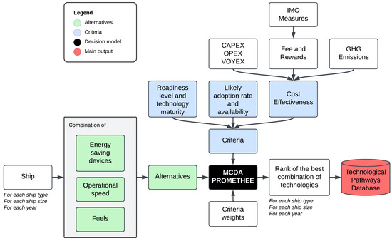
Figure 1.
Technological pathways model. Notes: The model evaluates combinations of technologies—namely energy-saving devices, operational speeds, and fuel types—for various ship types, sizes, and years. These combinations (shown in green) are assessed as Alternatives using a Multi-Criteria Decision Analysis (MCDA) method. The evaluation is based on Criteria (blue) such as cost-effectiveness, technology readiness, and adoption rates, which consider economic metrics (CAPEX, OPEX, VOYEX), IMO measures, and greenhouse gas (GHG) emissions. The decision model (black) ranks alternatives according to weighted criteria, identifying the best technology combination. The main output (red), stored in the Technological Pathways Database, provides a ranked set of optimized pathways per ship type, size, and year to support decision-making in maritime decarbonization.
The process begins with ship-specific input data, classified by ship type, size, and operational year. Different alternatives are generated as combinations of energy-saving devices (ESDs), operational speed adjustments, and alternative fuels, described in detail in Table 1. The effect of each ESD, operational speed, and alternative fuel, as well as how they are incorporated into the model is explained in Appendix B Evaluation criteria include readiness level and technology maturity, likely adoption rate and availability, and cost-effectiveness, which is influenced by CAPEX, OPEX, VOYEX, GHG emissions, and IMO measures such as fees and rewards.

Table 1.
Combination of alternative technologies considered in the model.
The decision model ranks the combinations of technologies based on weighted criteria to identify the most suitable technological pathways for each type, size, and year. The output of the MCDA model represents the simulated decision of a shipowner for a given ship type, size, and operational year, identifying the most suitable combination of technologies based on the three weighted criteria. This approach allows for ship-specific, year-specific decision-making, with the model dynamically adjusting to technology maturity, availability, and cost-effectiveness. The ranked results are stored in a technological pathways database, providing a comprehensive resource for the decision-making of sustainable shipping.
2.1.2. Ranking of the Technologies
Multi-Criteria Decision Analysis (MCDA) is a decision-making framework designed to evaluate and compare alternatives across multiple, often conflicting, criteria. In this study, MCDA is applied to rank the effectiveness of various GHG abatement technologies, including energy-saving devices, renewable fuels, speed-reduction measures, and market-based mechanisms, against a set of predefined criteria. Each criterion is assigned a weight, reflecting its relative importance, which is then incorporated into the evaluation to provide a balanced comparison of the technologies.
For this analysis, we employ the PROMETHEE (Preference Ranking Organization Method for Enrichment Evaluation) method, a widely used MCDA technique that ranks alternatives through pairwise comparisons based on their performance across the criteria [22]. PROMETHEE involves calculating preference indices and flows, which represent the outranking relationships between different technology options, ultimately producing a ranked list of GHG abatement measures.
Among various MCDA methods, PROMETHEE was selected due to its ability to handle complex decision-making contexts with a large number of alternatives and criteria, which is critical in the evaluation of maritime decarbonization technologies. Compared to AHP, which requires extensive pairwise comparisons and may become impractical with a large number of alternatives, PROMETHEE offers computational efficiency and scalability suitable for analyzing more than 10,000 technology combinations per vessel profile. Additionally, PROMETHEE allows for partial and complete ranking through the calculation of preference flows, providing a more nuanced evaluation than the simple aggregative scoring used in TOPSIS. Moreover, PROMETHEE can manage non-compensatory trade-offs between criteria, aligning with the need to balance cost-effectiveness, technology readiness, and adoption likelihood without overemphasizing any single dimension. These capabilities make PROMETHEE particularly well-suited for this study, where dynamic, year-by-year vessel-specific decision-making is required under uncertainty and evolving technological maturity. Further justification for PROMETHEE’s application, including its mathematical structure and advantages over other MCDA methods, is provided in Appendix D.
Here we considered three criteria to rank the combination of technologies, i.e., the readiness level (technology maturity), the likely adoption rate and availability, and the cost-effectiveness. Importantly, the shipowner decision to adopt a combination of technologies is not predefined or fixed, but rather emerges from the aggregation of individual ship-level decisions across the global fleet. Each year, the model simulates the decision of shipowners for specific ship types and sizes using MCDA rankings based on the three criteria.
Figure 2 shows the temporal evolution of the first two criteria—technology readiness and adoption likelihood—for various technologies from 2010 to 2035, as implemented in the model (MCDA inputs).
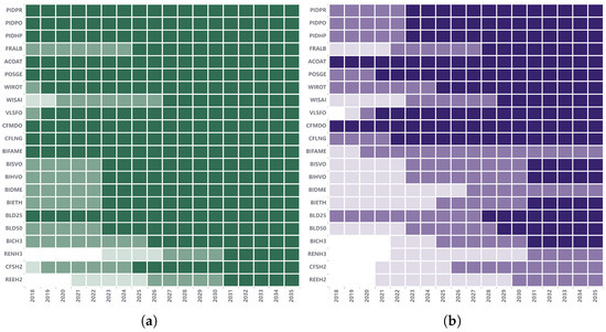
Figure 2.
Technology maturity and availability per year (2018–2035) based on [6,23,24,25,26,27]. (a) Readiness level and technology maturity. (b) Likely adoption rate and availability. Notes: Panel (a) shows the readiness level and maturity of the technologies based on technology readiness level (TRL). A rating of 0 (white) refers to measures that are not available, a rating of 1 (light green) refers to measures with a TRL less than 5, a rating of 2 (green) refers to a TRL of 5/6/7, and, a rating of 3 (dark green) refers to a TRL of 8/9; Panel (b) shows the likely adoption rate and availability. A rating of 0 (white) refers to technologies that are not available, a rating of 1 (light purple) refers to low likely adoption and low global availability, a rating of 2 (purple) refers to moderate likelihood of adoption and moderate global availability, and, a rating of 3 (dark purple) refers to high likely adoption rate and high availability.
Panel (a) shows the technology readiness levels (TRL), ranging from unavailable (white) to high maturity (dark green), while panel (b) displays the likely adoption rate and global availability, from unavailable (white) to high (dark purple). This visualization helps to assess the maturity and adoption trends of emerging technologies over time.
The cost-effectiveness of the combinations of technologies is the third and most important criterion. It is measured in terms of dollars per ton of CO2 equivalent abated (USD/ton CO2e) from a well-to-wake perspective (WTW). It is calculated by dividing the total CO2 emission savings over the remaining operational lifetime of the vessel (which varies according to the specific vessel analyzed) by the implementation costs associated with the technology. Implementation costs are defined as the sum of capital expenditures (CAPEX), operational expenditures (OPEX), voyage-related expenditures (VOYEX), and fees (FEES), minus any financial rewards or incentives (REWARD) that may apply.
Each ship’s cost components—CAPEX, OPEX, and VOYEX—are calculated based on ship type, size, operating profile (e.g., speed), and the specific technology considered. Since each actual ship travels a specific route and only one virtual sample ship is assessed for each combination of type, size, and age, the route distance is taken as a single average value for all virtual ships. This assumption is important because many variables are time-dependent, and at this stage, none of the virtual ships were yet connected to a specific trade flow. This approach allows us to assess the impact of each technology on the Total Cost of Ownership (TCO) [28,29,30,31,32].
In summary, the cost impact of adopting a GHG-reduction measure is estimated by analyzing three key factors: (i) changes in capital costs (CAPEX) associated with the implementation of each alternative, (ii) changes in voyage costs (VOYEX), primarily driven by variations in fuel consumption—whether using heavy fuel oil (HFO) or alternative marine fuels, and (iii) changes in operational and maintenance costs (OPEX) resulting from the adoption of new technologies.
The costs associated with adopting a given technology consider factors such as the potential loss of cargo space—resulting from the need for larger fuel tanks compared to conventional systems (e.g., diesel engines using HFO)—and/or increased travel times due to reduced vessel speeds. Consequently, the model accounts for the possible need for additional vessels to maintain the same transport capacity. In such cases, the corresponding costs—CAPEX, OPEX, and VOYEX—are proportionally allocated across the fleet. A detailed breakdown of these costs is provided in Appendix C.
The emission savings are determined on the basis of actual annual ton-miles delivered and the vessel’s energy consumption, as estimated through the model. Consequently, factors such as the size, type and age of the vessel significantly influence the overall cost-effectiveness assessment, as they affect both the operational characteristics and the potential emission reductions of the vessel. This comprehensive approach enables a multicriteria decision analysis (MCDA) to account for vessel-specific parameters when evaluating the economic and environmental viability of the technology.
The outcomes of the multicriteria decision analysis (MCDA) are strongly influenced by the weightings assigned to each criterion, as these weights represent the relative importance of each factor in the overall evaluation. Higher weights indicate a greater influence on the final decision, thus shaping the ranking and selection of technologies. For this study, a weight of 70% has been assigned to cost effectiveness, reflecting its primary significance in the evaluation. The remaining 30% are equally distributed, with 15% allocated to technology readiness level (maturity) and 15% to the likely adoption rate and availability. This weighting scheme was determined based on the practical decision-making criteria commonly used by shipowners, who prioritize economic viability when adopting new technologies. In the maritime industry, investment decisions are often driven by return on investment (ROI) and total cost of ownership (TCO), especially given the long operational lifetimes and high capital costs of vessels. Therefore, assigning a higher weight to cost-effectiveness reflects real-world priorities where economic feasibility is the dominant factor influencing technology uptake. While technology readiness and availability are also critical, they generally act as constraints rather than primary drivers of decisions. The weighting was applied uniformly across all vessel types and operating environments to maintain consistency and comparability across simulations.
2.2. World Trade Flow Simulation Model
The model starts from a baseline year (2018) using industry data and input parameters and forecasts the global fleet’s evolution through techno-economic modeling to assess the competitiveness of individual vessels in future scenarios. This approach considers the evolving energy efficiency of the fleet during the 2019–2035 period. Algorithms are used to simulate the annual decision-making processes of ship owners and operators concerning fleet management and operations. Figure 3 illustrates the comprehensive framework developed to simulate world trade flows. This framework integrates multiple datasets and processes to analyze trade dynamics, shipping activities, greenhouse gas (GHG) policies, technological pathways, costs, and emissions. The simulation begins with trade data, which encompass bilateral trade between 141 countries or regions (Appendix F.1) for 45 categories of tradeable goods (Appendix F.2), analyzed for each year and scenario. Trade flows are based on the same aggregation as used in the GTAP (Global Trade Analysis Project) is utilized in part II of this study, to calculate the economic and GHG emission impacts of the analyzed IMO medium-term measures. For details, see Pereda et al. [21] model [33]. Regarding global bilateral trade flows, the model utilizes UN Comtrade data, disaggregated by product, to estimate maritime trade volumes. The methodology described in Pereda et al. [34] is applied to derive maritime trade flows from total trade data, including ground and air transportation. An illustration of bilateral trade flows for the year 2019 is available in the Appendix F.4. The trade projections for 2019–2035 are based on population and GDP forecasts derived from the SSP2 scenario provided by the IPCC [35]. An essential aspect of the model is the correlation between the type of cargo and the corresponding ship used for transportation. For example, crude oil and iron ore are typically transported by oil tankers and bulk carriers in sizes commonly employed in the shipping market. Similarly, manufactured goods are generally carried by container ships.
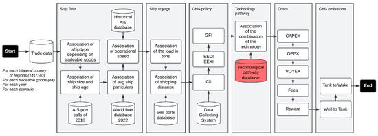
Figure 3.
World trade flow simulation model. Notes: The Technological pathway database (highlighted in red) represents the output of the Technological Pathway Model, which stores the best technology combinations for different scenarios and feeds this information into the model. All data associations and model steps are applied for each bilateral country or region pair (141 × 140), each of the 44 tradeable goods, each year, and each scenario.
The ship fleet module considers eight types of ship, categorized by different sizes, and five age categories of the ship, as detailed in Appendix E. This module links ship types to tradeable goods and associates ship size and age with AIS port call data from 2018. Operational speeds were derived from historical AIS data by ship type and size for the period 2018–2023, ensuring realistic modeling of vessel behavior during this time. Beyond 2023, ships are assumed to maintain their last observed average speed unless altered by scenario-specific measures. This assumption establishes a consistent baseline for evaluating the impact of speed-reduction strategies—such as slow steaming—which are introduced in the model as technical GHG-mitigation options. These scenarios simulate potential responses to varying economic conditions, including shifts in fuel prices and freight rates, thereby indirectly incorporating economic responsiveness into the model. Average ship particulars, such as dimensions and capacities, are sourced from the 2022 global ship fleet database.
The ship voyage module calculates cargo loads based on vessel capacity and type, employing cargo loading factors defined in the 2nd IMO GHG Study (Appendix E.3). Trade routes are linked to geographic shipping distances using a seaport database comprising approximately 1400 port terminals aggregated by region (Appendix F.3). The module further assesses the number of voyages needed and travel times, based on the ship’s average speed. The validation of the ship fleet profile, the total distance traveled, and the transport work is carried out using external datasets (Section 3.1).
The GHG policy module incorporates environmental metrics and standards, such as the Greenhouse Gas Fuel Intensity (GFI), the Energy Efficiency Design Index (EEDI), the Energy Efficiency Existing Ship Index (EEXI), and the Carbon Intensity Indicator (CII). The CII metric is statistically evaluated using data from the current ship and the Data Collecting System (DCS) for 2022.
In the technology pathway module, various technological solutions are evaluated by associating combinations of innovations described in the technological pathway database (see Section 2.1). This database, generated by the MCDA-based Technological Pathway Model, stores the optimized technology combinations per ship type, size, and operational year. These outputs serve as a dynamic input for the World Trade Flow Simulation Model, which assigns these optimal (or scenario-specific) combinations to vessels during simulation runs. This data flow enables realistic modeling of fleet-level decisions on technology adoption, emissions, and costs, ensuring consistency between the decision-making process and trade flow simulations across all scenarios. This interaction and data flow are illustrated in Figure 1 and Figure 3, where the Technological Pathways Database (highlighted in red) links both models.
The average renewal rate of the global fleet between 2012 and 2020, derived from IHS Maritime Trade data, shows fluctuations between 4.49% and 5.61% annually across vessel types and sizes, including bulk carriers, container ships and crude oil tankers. This renewal rate represents the proportion of new ships delivered each year as a percentage of the previous year’s total fleet size. Although there are variations between ship types and sizes, the model simplifies this by applying a constant annual fleet-renewal rate of 5%. This assumption ensures that the fleet is completely renewed over a 20-year period, aligning with a typical ship’s operational lifetime. Furthermore, the implementation of new technological pathways in the model assumes that 5% of the fleet adopts these advances annually, mirroring the renewal rate. This gradual integration of innovative solutions allows for a realistic projection of decarbonization pathways while maintaining alignment with historical fleet turnover rates. It is worth mentioning that the model does not currently simulate vessel upsizing, and instead models increased transport demand via an increased number of voyages by representative vessels per type and size class.
The cost module provides an economic breakdown that details CAPEX, OPEX, and VOYEX. It also includes considerations for fees and rewards arising from market-based measures. Finally, the GHG emissions module quantifies emissions from two perspectives, using data presented in Table A4: tank-to-wake emissions (TTW), which capture operational emissions directly associated with ship propulsion and energy use, and well-to-tank emissions (WTT), which account for upstream impacts of fuel production, processing, and transportation. It is important to note that costs, fees, rewards, and (GHG) emissions were previously evaluated to determine the cost-effectiveness of each technological combination within the MCDA framework. However, at this point, each virtual sample ship is already linked to a trade flow, which ensures that the travel distances are realistic and the results are more accurate.
Together, these interconnected modules form a robust simulation framework that comprehensively evaluates global trade flows, incorporating environmental and economic dimensions.
2.3. Simulation Matrix—Scenario Development
Table 2 summarizes the key characteristics of the scenarios considered in this study, highlighting their distinct approaches to greenhouse gas (GHG) reduction in the global shipping fleet. All GHG emissions in the scenarios are evaluated using a Well-to-Wake (WTW) perspective, encompassing both upstream and operational emissions associated with fuel production, processing, transport, and ship usage. Each scenario reflects a different combination of regulatory frameworks, operational strategies, and technological adoption pathways, providing a comprehensive analysis of potential outcomes under varying levels of intervention and market-based measures detailed in Appendix A.3. The following list details each scenario, explaining the specific policies, assumptions, and expected impacts on emissions and economic performance:
Table 2.
List of the scenarios considered in the study.
- REF—This scenario acts as the baseline, modeling the global shipping fleet without any new policies or measures aimed at reducing greenhouse gas (GHG) emissions. It reflects actual fleet data from 2018 to 2022 and projects that ships will continue operating at their current speeds through 2035. In this scenario, shipowners are assumed to not invest in energy-saving devices (ESD) or alternative fuels. The purpose of the REF scenario is to demonstrate the potential outcomes of a ‘business-as-usual’ approach, highlighting both the minimal financial investments and the highest potential emissions. It serves as a benchmark for comparing the impact of other, more proactive measures.
- BAUOPT—This scenario builds on current GHG regulations, incorporating short-term measures such as EEDI, EEXI (Appendix A.1), and CII (Appendix A.2) to promote the gradual decarbonization of the global fleet. It assumes an annual 2% reduction in carbon intensity up to 2035. The scenario evaluates all available technologies, assuming that shipowners consistently select the most effective combinations to comply with regulatory standards. BAUOPT explores the optimal scenario where shipowners make well-informed, cost-effective decisions, and shipyards renew 5% of the fleet annually. This scenario is key for understanding the potential of achieving maximum emissions reduction through rational investment and policy adherence.
- BAU20P—This scenario assumes the same regulatory environment as BAUOPT, including compliance with EEDI, EEXI, and CII. In this scenario, shipowners, on average, select combinations of technologies that are 20% below the cost-effectiveness of the optimal option determined by the MCDA ranking, introducing a level of non-optimality that simulates realistic decision-making under uncertainty. While energy-saving devices and alternative fuels remain optional in this scenario, it better reflects the real-world behavior where shipowners may not always make the most optimal investment choices. BAU20P illustrates the potential emissions outcomes when suboptimal decisions are made, offering a more realistic outlook compared to the idealized BAUOPT scenario.
- LEVY—In this scenario, a global carbon pricing mechanism, such as a levy on GHG emissions, is introduced to incentivize shipowners to adopt more aggressive decarbonization strategies. This includes reducing operational speeds, investing in energy-saving devices, and transitioning to alternative fuels. EEDI, EEXI, and CII remain in force, but the levy system provides additional financial motivation to adopt more advanced environmental technologies. The LEVY scenario explores how market-based measures (MBMs) like a carbon levy can accelerate the decarbonization of the shipping industry, highlighting the role of economic incentives in driving significant reductions in emissions through both operational and technological improvements.
- FCMOR—Similar to the LEVY scenario, FCMOR introduces an MBM, but it specifically focuses on a ‘Fuel Compliance Mechanism-Original’ (FCM-original). Like the LEVY scenario, FCMOR enforces compliance with EEDI, EEXI, and CII while examining how the adoption of alternative fuel policies can influence the shipping sector’s decarbonization efforts.
- FCMRE—Building on FCMOR, the FCMRE scenario features a revised version of the fuel consumption mechanism (FCM-revised). This version introduces a sustainability criteria for fuels, ensuring that only those with low WTW emissions are incentivized. While the core features remain, FCMRE tests the effectiveness of adjustments to the original mechanism, providing insights into how incremental policy changes can influence shipowner behavior and emissions outcomes.
- FEEBA—In this scenario, a feebate system is introduced. Under this system, ships that exceed specified emissions thresholds are required to pay a fee, while those that perform better than required can receive rebates. The FEEBA scenario encourages investments in energy-saving technologies, speed reduction, and alternative fuels. Compliance with EEDI, EEXI, and CII is mandatory (Appendix A.1 and Appendix A.2). This scenario investigates the potential effectiveness of financial incentives and penalties in accelerating decarbonization efforts, providing a balanced approach between enforcement and reward to promote significant emissions reductions.
2.4. Assumptions and Limitations
The model is built on a set of well-defined assumptions designed to balance computational feasibility with the complexity inherent in the decarbonization pathways in the maritime environment. Shipowner decision-making is simulated using a multi-criterion decision analysis framework (MCDA), prioritizing technology readiness, adoption likelihood, and cost-effectiveness, while excluding qualitative factors such as market advantages of early adoption. Technological combinations are structured in three dimensions: machinery and fuel supply, energy efficiency technologies, and operational speed. This yields approximately 10,752 options per vessel type, per year, per age, per route, and per scenario, providing a granular foundation for analysis. The model assumes a feasible transition to alternative fuels within the defined timelines, contingent on adequate global infrastructure and availability. Baseline data, which reflect the characteristics of the 2018 fleet and trade flows, underpin the framework, with auxiliary fuel standardized as marine gas oil (MGO) and a constant sea margin of 15% applied in all scenarios. For simplicity, emerging technologies such as carbon capture and storage (CCS) and pilot fuel oil are excluded, while gas transport is modeled exclusively via LNG carriers.
Despite its comprehensive approach, the model recognizes certain limitations associated with long-term forecasting. The precision of the projections depends significantly on assumptions about fuel prices, technology costs, and effectiveness of the reduction-factors that are inherently subject to geopolitical and economic uncertainties. Although global fleet specifications are based on 2018 data to ensure reliability, they may not fully capture minor variations in operational or technical parameters. Additionally, the model does not dynamically account for shifts in global trade flows or potential post-pandemic economic adjustments.
A further limitation relates to the assumption of a constant annual fleet-renewal rate of 5% across all ship types. While this reflects the global average observed over the past decade, it does not capture the heterogeneity in renewal rates between vessel categories, such as the typically higher turnover of container ships compared to bulk carriers. This simplification may affect the accuracy of decarbonization pathway projections at the ship-type level, although it preserves consistency and tractability for global-scale scenario analysis. Future work could enhance model fidelity by incorporating ship-type-specific renewal dynamics where data permit.
In the LEVY scenario where levy revenues are allocated externally to climate adaptation, RD&D, and administrative costs. The model currently does not simulate alternative redistribution mechanisms, such as reinvesting levy income directly into the maritime sector through subsidies or investment support. As a result, the potential impacts of revenue recycling on technology uptake, equity, and transition speed are not assessed in this version.
Furthermore, the model specifically distributes cargo among bulk carriers, oil tankers, container ships, conventional general cargo vessels, and gas carriers, representing more than 90% of the global fleet’s total tonnage (DWT). Other merchant vessels, such as cruise ships and offshore supply vessels, are not considered in this study. Likewise, the analysis does not cover emissions from service vessels, as they fall outside the scope of this research.
These inherent constraints underscore the challenges of predicting long-term maritime pathways.
3. Results and Discussion
This section presents the key findings of the study, starting with the validation of load and transport work to ensure the reliability of the modeling approach. The analysis then explores the evolution of GHG emissions under different policy scenarios, followed by an assessment of transport costs associated with these measures. Additionally, the impact of various policies on the adoption of alternative fuels and technologies is discussed. Finally, the results are compared with those from a similar model, providing context and validation for the study’s conclusions.
3.1. Validation of Load and Transport Work
The validation of annual transported load per ship type, as illustrated in Figure 4 and detailed in Table 3, demonstrates the reliability of the model developed in this study compared to data from UNCTAD and Clarksons. The results show a consistent distribution of transported loads across ship types, with bulk carriers dominating the total transported volume, followed by crude oil tankers and container ships. General cargo ships, LNG tankers, and chemical tankers account for smaller proportions, yet their contributions align closely with reference data.
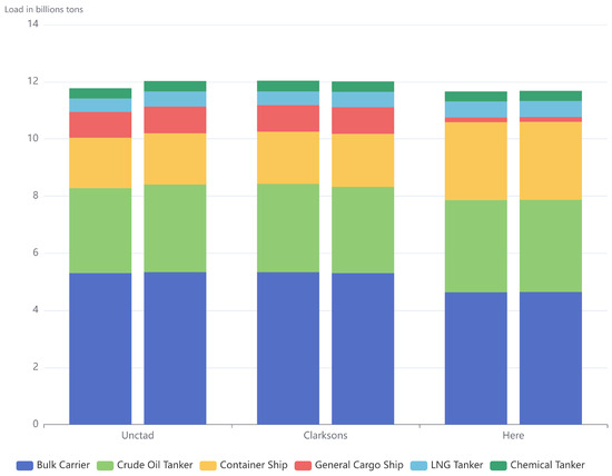
Figure 4.
Validation of annual transported load (in tons) per ship type for the years 2019 (left bars) and 2022 (right bars), compared against data from UNCTAD and Clarksons.
Table 3.
Comparison of the quantity of load transported by sea in tons per ship type for the year 2019.
Table 3 provides a detailed comparison of the quantities transported by each ship type for the year 2019. The total transported load estimated by the model deviates by only 1% and 3% from UNCTAD and Clarksons, respectively, confirming the robustness of the overall estimates. While bulk carriers, crude/product oil tankers, and chemical tankers show relatively small errors (ranging from 3% to 13%), larger discrepancies are observed for container ships (−54% relative to UNCTAD) and general cargo ships (82%). These discrepancies can be attributed to a modeling assumption where a portion of the load typically classified as general cargo is considered under container carriers. LNG tankers exhibit moderate deviations, with an error of −21% compared to UNCTAD. These variations highlight the challenges in accurately capturing the transported loads for certain ship types. In parallel, Figure 5 shows that the model prediction for annual seaborne transport work are closely aligned with UNCTAD and Clarksons, confirming its reliability in capturing trends and forecasting global maritime activity.
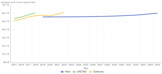
Figure 5.
Validation of annual total seaborne transport work, expressed in ton-nautical miles, compared with data from UNCTAD and Clarksons.
Overall, the comparison of results across datasets and the stability of the modal distribution over time (as shown for 2019 and 2022 in Figure 4) validate the model’s applicability for analyzing maritime transport trends. Despite some deviations for specific ship types, the agreement in total volumes and the relative consistency across ship types underline the model’s utility for policy development and maritime studies.
3.2. GHG Emissions
Figure 6 presents the well-to-wake (WTW) greenhouse gas (GHG) emissions trends for the different policy scenarios listed in Table 2. The reference scenario (REF) exhibits a nearly constant trajectory of emissions beyond the initial peak observed in the early 2020s, this reflects a balance between increasing trade volume and gradual improvements in fleet energy efficiency through renewal. This behavior highlights the lack of significant emission reduction without the implementation of energy efficiency measures, market-based policies, or alternative fuels.
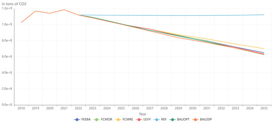
Figure 6.
Changes in WTW GHG emissions in tons of CO2 for each scenario. Notes: ‘REF’ stands for reference case; ‘BAUOPT’ means business as usual with optimal selection of technologies, ‘BAU20P’ means business as usual with the combinations of technologies that are 20% below the cost-effectiveness of the optimal option, ‘LEVY’ is a global carbon pricing mechanism, ‘FCMOR’ stand for Fuel Compliance Mechanism—Original, ‘FCMRE’ stand for Fuel Compliance Mechanism—Original, and ‘FEEBA’ refers to a feebate system composed of fees and a rebate.
In contrast, all other scenarios incorporating energy efficiency standards (EEDI, EEXI, and CII compliance), energy-saving devices (ESD), speed-reduction strategies, and alternative fuels show a consistent downward trend in emissions over time. Among these, the scenarios that include a market-based measure (MBM) policy—namely, LEVY (43%), FCMOR (43%), and FEEBA (42%) demonstrate similar reductions in GHG emissions by 2035, with the exception of FCMRE, which achieves a slightly lower reduction of 38%. This suggests that while market-based mechanisms generally lead to significant decarbonization, FCMRE may be less effective than the other MBM policies.
The LEVY scenario results in a steady decline in emissions, comparable to the flexible mechanisms (FCMOR and FCMRE). However, the FCMRE scenario underperforms slightly relative to the FCMOR and LEVY cases, indicating that the modifications introduced in this revised fuel-cycle mechanism may not be as effective in driving emission reductions. The FEEBA scenario achieves a similar reduction in GHG emissions over time. The scenarios BAUOPT (44%) and BAU20P (44%) also show similar reductions in emissions until 2035, being slightly more effective.
Overall, these findings indicate that while all regulatory scenarios lead to substantial and nearly equivalent reductions in GHG emissions by 2035, the key differentiating factors are associated with other criteria analyzed in the following section such as the economic implications and the pace of technological transitions in fuel choices and operational strategies.
3.3. Transport Cost
Figure 7 illustrates the evolution of total costs in USD for each MBM scenario (LEVY, FCMOR, FCMRE, and FEEBA) while distinguishing five key cost components (CAPEX, OPEX, VOYEX, TAX, and REWARD). In the LEVY scenario (Figure 7a), TAX costs increase progressively over time as carbon pricing mechanisms become more stringent, while CAPEX and OPEX slightly increase as the other MBMs. Notably, this scenario lacks any REWARD incentives, meaning shipowners bear the full cost of compliance. The FCMOR scenario (Figure 7b) follows a similar cost trajectory, but the introduction of REWARD mechanisms offsets part of the taxation burden, leading to lower cumulative costs compared to LEVY. The FCMRE scenario (Figure 7c) exhibits a cost trend similar to FCMOR, though with a higher reduction in TAX contributions by 2035. However, in the current configuration, the rewards are higher than TAX, suggesting that some adjustments of the mechanism are necessary to achieve a better balance between taxation and incentive (rewards should not overcome taxes). The most distinct cost structure is observed in the FEEBA scenario (Figure 7d). Unlike the other MBM policies, FEEBA includes a significant proportion of financial incentives, suitably mitigating the impact of taxation. While TAX costs still rise over time, their overall effect is less pronounced due to the simultaneous increase in REWARD allocations.
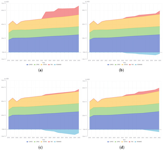
Figure 7.
Changes in costs in USD for each scenario. (a) LEVY. (b) FCMOR. (c) FCMRE. (d) FEEBA. Notes: ‘LEVY’ is a global carbon pricing mechanism, ‘FCMOR’ stand for Fuel Compliance Mechanism—Original, ‘FCMRE’ stand for Fuel Compliance Mechanism—Original, and ‘FEEBA’ refers to a feebate system composed of fees and a rebate.
The primary differences between these scenarios lie in the balance between TAX and REWARD. While LEVY imposes a significant financial burden without compensation, FEEBA, FCMOR, and FCMRE introduce mechanisms that help alleviate these costs, making compliance more economically manageable. CAPEX and OPEX, on the other hand, remain relatively stable across all scenarios, while VOYEX varies slightly, indicating that the variations in total cost primarily stem from the structure of the MBM policy rather than differences in investment or operational expenditures.
In complement, Figure 8 provides a comparative analysis of the total costs sum (CAPEX + OPEX + VOYEX + TAX) and financial incentives (REWARD) across different policy scenarios. Panel (a) presents the evolution of total costs isolated while panel (b) isolates the evolution of financial rewards under selected market-based measure (MBM) policies. In panel (a), the total costs for all scenarios increase over time, driven by the cumulative impact of investment in decarbonization technologies, operational expenses, and regulatory measures. The REF scenario maintains the lowest cost trajectory, as it does not incorporate any additional compliance expenditures. The BAUOPT and BAU20P scenarios exhibit slightly higher costs by 2035, respectively 5% and 19%, due to the implementation of energy-saving technologies and operational adjustments, such as speed reduction. However, the most notable increases in costs are observed in the MBM policy scenarios, particularly LEVY, which experiences the steepest rise of 46% by 2035. The other MBM scenarios, including FCMOR, FCMRE, and FEEBA, follow similar trajectories, respectively 30%, 25% and 32% by 2035, but their cost growth is moderated by financial incentives, as reflected in panel (b).
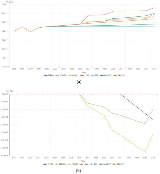
Figure 8.
Comparison of costs and rewards in USD among the scenarios. (a) Total costs (CAPEX + OPEX + VOYEX + TAX). (b) REWARD. Notes: ‘REF’ stands for reference case; ‘BAUOPT’ means business as usual with optimal selection of technologies, ‘BAU20P’ means business as usual with the combinations of technologies that are 20% below the cost-effectiveness of the optimal option, ‘LEVY’ is a global carbon pricing mechanism, ‘FCMOR’ stand for Fuel Compliance Mechanism—Original, ‘FCMRE’ stand for Fuel Compliance Mechanism—Original, and ‘FEEBA’ refers to a feebate system composed of fees and a rebate.
Panel (b) highlights the evolution of financial rewards under the FEEBA, FCMOR, and FCMRE scenarios, in contrast to the LEVY scenario, which does not include incentives. The negative values indicate cost reductions due to subsidies or rebates. The FCMRE scenario demonstrates the highest level of rewards over time, offsetting a significant portion of the total compliance costs. The FCMOR and FEEBA scenarios also exhibit financial incentives, though to a lesser extent. This suggests that the revised fuel-cycle mechanism (FCMRE) includes stronger financial compensation mechanisms compared to the original version (FCMOR).
The results demonstrate that while all market-based measure (MBM) policies achieve similar reductions in GHG emissions, their economic impacts differ significantly, influencing their feasibility and adoption by the shipping industry. The LEVY scenario imposes the highest compliance costs due to the absence of financial incentives, placing a greater financial burden on shipowners. In contrast, FEEBA and the fuel-cycle mechanisms (FCMOR and FCMRE) introduce financial rewards that help offset compliance costs, making these policies more economically sustainable. Among them, the FEEBA scenario appears to offer the most balanced approach by integrating penalties with incentives, potentially facilitating broader adoption of decarbonization measures.
The effectiveness of each policy is therefore not solely determined by its capacity to reduce emissions but also by its ability to distribute costs and incentives in a way that ensures both regulatory compliance and financial feasibility. Policies that rely solely on taxation mechanisms may face resistance due to their high economic impact, while those that incorporate financial rewards can alleviate costs and encourage the transition to low-emission technologies. These findings highlight the importance of a balanced approach that combines carbon pricing with well-designed financial incentives to accelerate decarbonization while minimizing economic disruptions in the shipping sector.
3.4. Fuels Adoption
Figure 9 illustrates the projected changes in energy consumption, measured in megajoules (MJ), by fuel type in six different decarbonization policy scenarios from 2018 to 2035. Each panel represents a distinct scenario, incorporating various policy measures and market responses influencing the transition rate from conventional fuels to alternative energy sources.
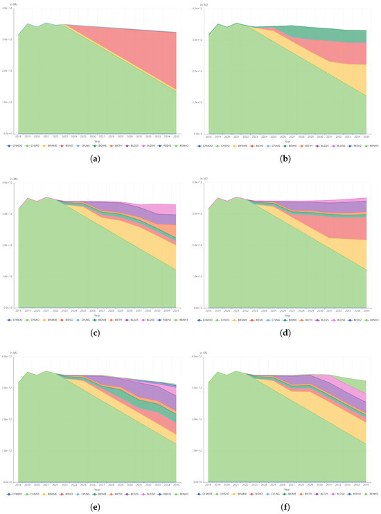
Figure 9.
Changes in fuel adoption in MJ for each scenario. (a) BAUOPT. (b) BAU20P. (c) LEVY. (d) FCMOR. (e) FCMRE. (f) FEEBA. Notes: CFMDO is the conventional Marine Diesel Oil, CHSFO is the conventional bunker, BIDME is the Dimethyl Ether, BIETH is the Bioethanol, BIFAME is the Fatty Acid Methyl Esters-Biodiesel, BISVO is the Straight Vegetable Oil, BLD25 is a blended fuel with 25% straight vegetable oil (SVO) and 75% very low sulfur fuel oil (VLSFO), while BLD50 increases the biofuel content to 50%, further reducing greenhouse gas emissions.
In panel (a), BAUOPT scenario, a gradual phase-out of conventional heavy fuel oil (CHSFO) is observed, while biofuels, particularly BISVO (red), progressively assume a dominant role. Biodiesel (BIFAME) plays a minor role, indicating limited diversification in fuel options. This outcome is explained by the assumption that, in this scenario, shipowners prioritize the most cost-effective solutions to achieve decarbonization goals without constraints on fuel availability. As a result, fossil fuel dependency remains significant, with CHSFO continuing to play an important role even in 2035.
The BAU20P scenario, shown in panel (b), results in a more balanced distribution of selected biofuels, including BISVO, BIFAME, and BIDME, compared to BAUOPT. A critical observation from this scenario is that the model does not select any of the other sustainable fuel options, such as green methanol, green ammonia, or green hydrogen. This finding underscores the necessity of additional greenhouse gas (GHG) measures to motivate the adoption and integration of a broader range of renewable fuels.
Panel (c) presents the LEVY scenario, which exhibits a similar decline in CHSFO consumption. This scenario also shows a notable increase in the adoption of bio-ethanol (BIETH) and renewable biodiesel (BIFAME), leading to a more diversified fuel mix compared to the business-as-usual scenarios. The increased adoption of multiple alternative fuels highlights the growing influence of financial mechanisms in promoting fuel diversification.
The FCMOR scenario, shown in panel (d), further reinforces this transition by incorporating a substantial share of low-carbon synthetic fuels, particularly BLD25 and BLD50. This shift suggests a stronger regulatory push towards alternative fuel adoption, reducing dependence on conventional fossil fuels.
The FCMRE scenario, displayed in panel (e), demonstrates a more balanced adoption of renewable fuels, with a significant presence of BLD25 and BLD50 alongside BISVO, BIETH, BIFAME, and BIDME. This scenario also shows a noticeable reduction in absolute energy consumption, indicating the widespread implementation of slow steaming and energy efficiency technologies including wind-assisted ship propulsion. The results suggest that, under FCMRE, shipowners are not only shifting towards alternative fuels but are also investing in operational and technological strategies to further reduce emissions and improve energy efficiency.
Finally, the FEEBA scenario, presented in panel (f), produces results similar to those observed in the FCMRE scenario. Under this scenario, biofuels such as BISVO, BIFAME, and BIETH dominate the new energy supply, with substantial contributions from blended fuels, including BLD50 and BLG25. The increased reliance on these fuels suggests that economic incentives, such as feebate mechanisms, effectively promote the transition to low-carbon energy sources. Additionally, the more significant reduction in absolute energy consumption highlights the succeeded encouragement for operational and technological strategies.
Across all scenarios, the decline in CHSFO consumption is evident; however, the rate of reduction is directly influenced by the fleet-renewal rate constraint. In scenarios with more stringent regulatory measures, such as LEVY, FCMOR, FCMRE, and FEEBA, the shift away from fossil fuels is accompanied by a significant increase in the adoption of biofuels, particularly BISVO, BIFAME, BIETH, and various fuel blends. A critical observation is that the model never selects more expensive sustainable fuels, such as biomethanol, green ammonia, or green hydrogen by 2035, indicating that additional policy interventions or technological advancements may be necessary to make these options more economically viable.
Overall, Figure 9 underscores the essential role of policy design in shaping the future energy landscape of maritime transport. The analysis reveals that regulatory and financial mechanisms significantly accelerate the adoption of alternative fuels. The findings suggest that achieving full decarbonization in the sector will require a combination of market incentives, stringent policies, and strategic investments in renewable energy infrastructure.
3.5. Technologies Adoption
Figure 10 illustrates the evolution of technology adoption in the maritime sector under different policy scenarios. The adoption trends for energy-saving devices, operational speed adjustments, and wind-assisted propulsion systems vary significantly across the six scenarios, reflecting the impact of regulatory and economic incentives on fleet behavior.
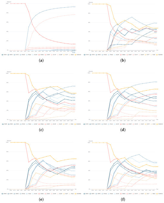
Figure 10.
Changes in technology adoption in percent for each scenario. (a) BAUOPT. (b) BAU20P. (c) LEVY. (d) FCMOR. (e) FCMRE. (f) FEEBA. Notes: Energy efficiency devices are represented using a blue gradient, where PIDPR denotes pre-swirl devices, PIDPH refers to high-efficiency propellers, PIDPO represents post-swirl devices, POSGE indicates shaft generators, FRALB corresponds to air lubrication with microbubbles, and ACOAT signifies advanced hull coatings. Operational speed alternatives are depicted using a red gradient, where OSBAU represents the business-as-usual operational speed of the vessel, OS05P indicates a 5% reduction from the current operational speed, OS10P corresponds to a 10% reduction, and OS20P represents a 20% reduction. Wind-assisted propulsion systems are shown using an orange gradient, where FLETT represents Flettner rotors, RIGID corresponds to rigid sails or wings, and NOWIND indicates the absence of a wind-assisted propulsion system. See Appendix B for details.
In panel (a), representing the BAUOPT scenario, the adoption of energy efficiency measures remains limited, with a large and global adoption of shaft generators (POSGE) emerging as the dominant technology. A sharp decline in business-as-usual operational speed (OSBAU) is observed, with a simultaneous increase in slow steaming strategies, particularly at a 20% speed reduction (OS20P). However, the uptake of wind-assisted propulsion remains marginal, suggesting that without regulatory pressure, shipowners prioritize fuel-saving technologies over wind-assisted propulsion.
Panel (b), depicting the BAU20P scenario, follows a similar trend to BAUOPT but exhibits a more diversified technology adoption pattern. Shaft generators (POSGE) still lead the adoption curve, while other energy efficiency measures such as pre-swirl devices (PIDPR), high-efficiency propellers (PIDPH), and hull coatings (ACOAT) gain traction. Wind-assisted propulsion, particularly rigid sails (RIGID) and Flettner rotors (FLETT) see a higher increase compared to the BAUOPT scenario, indicating a shift towards a broader range of fuel-saving strategies.
The LEVY scenario, shown in panel (c), accelerates the adoption of energy-saving technologies, with POSGE, PIDPR, and PIDPH reaching higher adoption levels than in the previous scenarios. The impact of the carbon levy mechanism also leads to a more significant uptake of slow steaming measures, particularly the 5%, 10%, and 20% speed reductions (OS05P, OS10P and OS20P). Wind-assisted propulsion becomes slightly less attractive under this scenario compared to BAU20P scenario.
In panel (d), corresponding to the FCMOR scenario, a broader range of technologies is adopted more extensively. The adoption of pre- and post-swirl devices (PIDPR and PIDPO), hull coatings (ACOAT), and air lubrication systems (FRALB) increases significantly compared to the BAU scenarios. Slow steaming continues to play a key role in emission-reduction strategies, with OS05P adoption surpassing 30% by 2035. Wind-assisted propulsion also experiences a consistent adoption, reflecting a greater shift towards multi-technology solutions.
The FCMRE scenario, depicted in panel (e), follows a similar trajectory to FCMOR but places a stronger emphasis on operational measures. While the adoption of shaft generators (POSGE) is lower compared to other scenarios, this is offset by a significant increase in the adoption of Flettner rotors for wind-assisted propulsion, which reaches its highest level under this policy framework. This shift suggests a greater reliance on renewable propulsion technologies as part of the decarbonization strategy.
Finally, panel (f), representing the FEEBA scenario, exhibits similar results with a large adoption of wind-assisted propulsion and slow steaming strategies, particularly OS05P and OS10P. The adoption of energy-saving devices, operational measures, and wind-assisted propulsion reaches its highest combined levels, indicating that feebate mechanisms provide strong incentives for the adoption of multiple strategies simultaneously. Although shaft generators (POSGE) remain the most widely adopted technology, wind-assisted propulsion systems, particularly rigid sails, and Flettner rotors, gain significant traction. This scenario suggests that a well-structured feebate system effectively encourages the deployment of various decarbonization measures, leading to a more sustainable and technologically diversified fleet.
Across all scenarios, a clear shift away from business-as-usual operational speeds is evident, with slow-steaming strategies gaining substantial adoption. Energy efficiency technologies, particularly shaft generators, pre-swirl devices, and high-efficiency propellers, consistently emerge as preferred options due to their direct impact on fuel savings. The adoption of wind-assisted propulsion varies significantly across scenarios, with its highest uptake observed in the LEVY and FEEBA scenarios, where financial mechanisms create a stronger incentive for its implementation.
Overall, Figure 10 highlights the critical role of policy design in shaping the future adoption of energy-saving technologies in the maritime industry. While business-as-usual scenarios lead to gradual and limited technology adoption, regulatory interventions such as carbon levies, flexible compliance mechanisms, and feebate systems significantly accelerate the uptake of alternative propulsion and operational efficiency measures. These findings emphasize the importance of implementing comprehensive and adaptive policy frameworks to drive maritime decarbonization.
3.6. Comparison with a Similar Model
The methodologies employed in this study and in IMO [37] share similarities in evaluating greenhouse gas-reduction scenarios and their impacts on maritime transport but differ in key assumptions and approaches. Both studies analyze WTW reductions and transport costs under various scenarios and adopt comparable regulatory frameworks, such as EEDI, EEXI, and CII. However, this study incorporates a constrained retrofitting approach, a detailed technology readiness assessment, and a broader range of fuel options based on recent data. Unlike [37], the present methodology accounts for regional trade flows and provides a pathway model to evaluate the adoption of energy efficiency measures individually, ensuring a higher level of granularity. Additionally, this study limits fleet retrofitting to 5% per year and explicitly incorporates the availability of fuels and regional variations, providing a more comprehensive and realistic analysis of decarbonization pathways.
Table 4 presents a comparison of the Well-to-Wake (WTW) reduction and transport cost increase for the year 2030 under different scenarios, comparing the results of this study with those published in [37]. The WTW reductions range from −25% to −27% in this study, closely aligning with the results from [37], which range from −21% to −23%, demonstrating the consistency and accuracy of the model in estimating emissions reductions.
Table 4.
Comparison of the WTW reduction and transport cost increase for 2030 with results published by [37].
The cost intensity, representing the total annual costs associated with operational and fuel expenses, as well as regulatory incomes and expenses, shows a similar level of agreement between the two studies. Cost increases range from 14% to 38% in this study, compared to 16% to 40% in [37]. Notably, the scenarios with no flexibility (LEVY and FEEBAT) result in higher cost increases, while scenarios with flexibility (FCMOR and FCMRE) exhibit relatively lower costs.
Overall, the comparison highlights the robustness of the current model in reproducing both emissions reductions and cost impacts across varying policy scenarios. The close alignment with [37] further validates the assumptions and methodologies employed in this study, supporting its use for evaluating future decarbonization strategies in maritime transport.
4. Conclusions
This study developed a comprehensive modeling framework to evaluate technological pathways for decarbonizing maritime transport, integrating Multi-Criteria Decision Analysis (MCDA) with techno-economic simulations. The results indicate that while technical and operational measures, such as slow steaming and energy-saving devices, can reduce emissions by up to 44%, market-based mechanisms (MBMs) significantly accelerate the transition to alternative fuels. Among the policy scenarios analyzed, flexible compliance mechanisms (FCMRO and FCMRE) and feebate systems (FEEBA) result in emissions reductions of 38% and 42%, respectively, by 2035, while a strict carbon levy (LEVY) achieves a 43% reduction but imposes the highest compliance costs, increasing transport costs by 46%. The study also reveals that shipowners prioritize biofuels such as BISVO, BIFAME, and blended fuels (BLD50), while higher-cost alternatives like green hydrogen, biomethanol, and ammonia remain economically unviable without additional policy support.
In comparing the different scenarios, the most decisive factor in reducing emissions across all policy frameworks is the implementation of energy efficiency measures, particularly shaft generators and slow steaming. These measures consistently yield significant emission reductions, even in the absence of alternative fuels. Market-Based Measures such as LEVY and FEEBA drive further reductions by incentivizing broader fuel diversification, notably increasing the adoption of biofuels like BISVO and BIFAME. However, LEVY imposes higher costs without rewards, while FEEBA balances compliance costs with financial incentives, facilitating smoother adoption. Flexible mechanisms (FCMOR, FCMRE) also reduce emissions effectively but require careful calibration of taxes and rewards to avoid excessive subsidies. Overall, technical and operational measures form the foundation of emissions reduction, while MBMs are pivotal for accelerating fuel transition. A combination of both is essential for achieving cost-effective and realistic decarbonization.
This study bridges a critical gap in maritime decarbonization research by offering a holistic assessment of technological and economic trade-offs, integrating regulatory impacts and cost dynamics. Unlike previous studies that focus on isolated aspects such as fuel transition or efficiency measures, our work presents a multi-dimensional evaluation incorporating vessel-specific constraints, fuel market dynamics, and policy interventions. The findings inform regulatory strategies and investment decisions by demonstrating the effectiveness of different MBMs in achieving emissions reductions while maintaining economic viability. This research also provides a robust framework that can be adapted to future policy scenarios, ensuring its relevance for academia, industry, and regulatory bodies.
While this study provides a comprehensive assessment, it relies on a constrained fleet-renewal rate (5%) and assumes static fuel availability, which may not fully capture the complexities of real-world fuel infrastructure development. Additionally, the economic feasibility of alternative fuels is subject to evolving market conditions and policy frameworks, necessitating continuous updates to the model. Future research should explore real-time data integration, enhanced modeling of regional fuel infrastructure constraints, and the inclusion of emerging technologies such as onboard carbon-capture and nuclear propulsion systems to refine predictions and improve decision-making.
Achieving zero-emission maritime transport requires a combination of regulatory measures, financial incentives, and industry-wide technological investments. The study underscores that well-structured MBMs can significantly reduce emissions without imposing excessive economic burdens, but their design must ensure cost distribution fairness and avoid unintended market distortions. Given the substantial variability in policy effectiveness and cost implications observed in this study, it is crucial to conduct thorough impact assessments before implementation. Policymakers must rigorously evaluate different policy configurations and parameter settings—such as levy rates, subsidy levels, and fleet-renewal constraints—to ensure that regulatory frameworks drive the intended environmental benefits without disproportionately affecting specific market segments. Furthermore, industry stakeholders should engage in proactive research and scenario testing to anticipate potential challenges and infrastructure needs, ensuring that alternative fuel adoption is both technically feasible and economically viable in the long term. Without such preemptive analysis, there is a risk of policies being either too lenient to drive meaningful change or too stringent to be practical, leading to economic inefficiencies and resistance from the shipping industry. To enhance the model’s applicability and forward-looking capability, we are currently extending the simulation horizon to 2050, allowing for a more comprehensive analysis of long-term decarbonization pathways and the evolving impacts of regulatory frameworks, fuel infrastructure development, and emerging technologies. This future extension will support more detailed scenario planning and provide stakeholders with practical insights for navigating the mid- to long-term transition to zero-emission shipping.
Author Contributions
Conceptualization, J.-D.C. and P.C.P.; Data curation, J.-D.C., L.F.A. and P.C.P.; Formal analysis, J.-D.C., C.H.M., L.F.A., A.L. and P.C.P.; Funding acquisition, J.-D.C. and P.C.P.; Investigation, J.-D.C., C.H.M., L.F.A. and P.C.P.; Methodology, J.-D.C., C.H.M., L.F.A., A.L. and P.C.P.; Project administration, J.-D.C. and P.C.P.; Software, J.-D.C., C.H.M. and L.F.A.; Supervision, J.-D.C.; Validation, J.-D.C., C.H.M., L.F.A., A.L. and P.C.P.; Visualization, J.-D.C.; Writing—original draft, J.-D.C., C.H.M. and L.F.A.; Writing—review & editing, J.-D.C., C.H.M., L.F.A., A.L. and P.C.P. All authors have read and agreed to the published version of the manuscript.
Funding
This study was partially funded by the Coordination for the Improvement of Higher Education Personnel (CAPES-Brazil), finance code 001, and the National Council for Scientific and Technological Development (CNPq-Brazil), under grants 405923/2022-8 (J.D.C.) and 309238/2020-0 (J.D.C.). We also acknowledge the financial support from the Institute of Economic Research Foundation (FIPE) through Project 5705 (P.P.), as well as research grants from CNPq 304221/2022-8 (P.P.) and FAPESP 2014/50848-9 (P.P.). The opinions, hypotheses, conclusions, and recommendations expressed in this paper are solely those of the authors and do not necessarily reflect the views of the funding agencies.
Institutional Review Board Statement
Not applicable.
Informed Consent Statement
Not applicable.
Data Availability Statement
Data are unavailable due to privacy restrictions.
Acknowledgments
We sincerely thank everyone who contributed to the development of this paper, as well as the entire Paula Pereda team for their support. Any remaining errors are solely our responsibility.
Conflicts of Interest
The authors declare no conflicts of interest. The funders had no role in the design of the study; in the collection, analyses, or interpretation of data; in the writing of the manuscript; or in the decision to publish the results.
Abbreviations
The following abbreviations are used in this manuscript:
| CII | Carbon Intensity Indicator |
| EEDI | Energy Efficiency Design Index |
| EEXI | Energy Efficiency Existing Ship Index |
| FCM | Flexibility Compliance Mechanism |
| FCU | Flexibility Compliance Units |
| GFI | GHG Fuel Intensity |
| IMO | International Maritime Organization |
| IMSF&F | International Maritime Sustainable Fuels and Fund |
| IPCC | Intergovernmental Panel on Climate Change |
| LDC | Least Developed Countries |
| MBM | Market-based measure |
| MEPC | Marine Environment Protection Committee |
| SEEMP | Ship Energy Efficiency Management Plan |
| TTW | tank-to-wake |
| UN | United Nations |
| WTT | well-to-tank |
| WTW | well-to-wake |
| ZEF | zero-emission fuel |
| ZESIS | Zero-Emission Shipping Incentive Scheme |
| ZEV | zero-emission vessel |
| GHG | greenhouse gas |
| MCDA | Multiple Criteria Decision Analysis |
| PROMETHEE | Preference Ranking Organization Method for Enrichment Evaluation |
| ESD | energy-saving devices |
| PIDPR | pre-swirl devices |
| PIDPO | post-swirl devices |
| PIDHP | and high-efficiency propellers |
| FRALB | reduction of skin friction by air lubrication |
| ACOAT | reduction of skin friction by texture of the hull surface |
| WASP | wind-assisted ship propulsion |
| WIROT | wind-assisted ship propulsion by Flettner rotors |
| WISAI | wind-assisted ship propulsion by rigid sails or wings |
| POSGE | shaft generators or power take-off |
| OSBAU | business as usual operational speed of the vessel |
| OS05P | 5% reduction from the business as usual operational speed of the vessel |
| OS10P | 10% reduction from the business as usual operational speed of the vessel |
| OS20P | 20% reduction from the business as usual operational speed of the vessel |
| VLSFO | Very Low Sulphur Fuel Oil |
| CFMDO | Marine Diesel Oil |
| CFLNG | refers to Liquefied Natural Gas |
| BIFAME | Fatty Acid Methyl Esters |
| BISVO | Straight Vegetable Oil |
| BIHVO | Hydrotreated Vegetable Oil |
| BIDME | Dimethyl Ether |
| BIETH | Ethanol |
| BLD25 | fuel consisting of a blend of 25% SVO and 75% VLSFO |
| BLD50 | fuel consisting of a blend of 50% SVO and 50% VLSFO |
| SVO | Straight Vegetable Oil |
| BICH3 | BioMethanol from gasification of biomass |
| RENH3 | Green Ammonia from Hydrogen |
| CFSH2 | Grey hydrogen from steam reforming of natural gas (compressed) |
| REEH2 | Green hydrogen from electrolysis using renewable energy (compressed) |
| TRL | technology readiness level |
| OPEX | operational expenditure |
| CAPEX | capital expenditure |
| VOYEX | voyage expenditure |
| GTAP | Global Trade Analysis Project |
| SSP2 | Shared Socioeconomic Pathway 2 |
| GDP | Gross Domestic Product |
| AIS | Automatic Identification System |
| DCS | Data Collecting System |
| FEEBA | Feebate system |
| MGO | Marine Gas Oil |
| CCS | carbon capture and storage |
| LNG | liquefied natural gas |
| UNCTAD | United Nations Conference on Trade and Development |
| BAUOPT | scenario considering business as usual and the selection of the most effective technological combinations |
| BAU20P | scenario considering business as usual and the selection of technological combinations 20% below the best available option |
| FCMOR | Fuel Compliance Mechanism-original |
| FCMRE | Fuel Compliance Mechanism-revised |
Appendix A. GHG Measures
Appendix A.1. Energy Efficiency Design Index (EEDI) and Energy Efficiency Existing Ship Index (EEXI)
EEXI is a measure to assess the design energy efficiency of existing ships and its attained value () is computed by the same equation used to the attained EEDI () for new ships [38]. Either for EEDI or EEXI, the attained value of the index ( or ) has to be lower or equal to a required value of the index ( or ) so that a ship can meet the requirement. Ships falling into the scope of the EEDI requirement can use their as the if the value of the former is equal to or less than the required EEXI (). Owing to unavailable data and the comprehensiveness of the approach, the formulation used here omitted the various correction factors usually considered for accuracy regarding specific design elements. Thus, both indexes’ attained value is calculated by Equation (A1), a simplification of the complete equation in [39]. More details about calculation may be found in [9].
The mass flow rates for the main and auxiliary engines ( and ) must be considered for 75% main engine maximum continuous rating (MCR). Accordingly, represents the ship’s reference speed when the main engines are at 75% MCR. Capacity is dead-weight tonnage (DWT) for all ship types, except for container ships, whose capacity is 70% DWT due to the containers’ weight. The conversion factor and link fuel consumption to CO2 emissions for the main and auxiliary engines, respectively. The main characteristics of the fuels used in this study, including the conversion factor , are detailed in Table A4. The present evaluation considers the same fuel type for the main and auxiliary engines to simplify the calculation process. More details about the main and auxiliary engines fuel consumption can be found in [40]. This approach provides a basic assessment of the indices, highlighting the need for detailed data for a more accurate evaluation.
The required EEDI () is calculated based on a reduction factor (X) and the EEDI reference line (), as per Equation (A2). Values for factor X depend on ship type and size besides the EEDI phase, which depends on ship delivery date [38]. Similarly, the required EEXI () is calculated based on another reduction factor (Y) and the same , as given in Equation (A3). That factor Y holds different values depending on ship type and size, as listed in [38]. Finally, is computed by Equation (A4), where the parameters a, b, and c depend on ship type and capacity, as also documented in [38].
Appendix A.2. Carbon Intensity Indicator (CII)
In its most simple form, the annual operational carbon intensity indicator attained () from individual ships of 5000 GT or greater is calculated as the ratio of the total mass of emitted to the total transport work carried out in a given calendar year. The main difference from EEDI/EEXI attained is that CII attained considers the total fuel consumption and total distance traveled () throughout the year, regardless of the main engine load and ship speed. This means that there is no reference operational condition, resulting in Equation (A5), where and are respectively the fuel consumption of main and auxiliary engines, and is the distance traveled. A formulation accounting for voyage adjustments and correction factors is provided in [12] but was not the one applied here due to unavailable data.
Like the previous design indices, is compared to a required value. The required annual operational carbon intensity indicator () is calculated by Equation (A6) based on the reference value () and the time-reduction factor (Z). The reduction factor indicates the tightening of carbon efficiency requirements over time and is fixed by regulation, with plans for reassessment in 2027. Therefore, the values in Table A1 are based on the regulation until 2026, and our assumptions are applied from 2027 onward. The reference line for the carbon intensity indicator () is formulated as in Equation (A7), where a and c are parameters depending on ship type and capacity, given in [41].
In contrast to EEDI and EEXI, which result in a simple compliance or non-compliance outcome, the operational carbon intensity indicator involves levels when comparing and . Based on this comparison, the ship is assigned a ranking label from A to E, representing major superior (A), minor superior (B), moderate (C), minor inferior (D), or inferior (E) performance level. Four boundaries are defined for the five-grade rating mechanism to facilitate the assignment of ratings. Thus, a rating can be assigned by comparing with the boundary values given in [42], depending on ship type and capacity.
Table A1.
Reduction factor Z for the CII relative to the reference line.
Table A1.
Reduction factor Z for the CII relative to the reference line.
| Year | 2020 | 2021 | 2022 | 2023 | 2024 | 2025–2030 | 2030–2035 |
|---|---|---|---|---|---|---|---|
| Z | 1 | 2 | 3 | 5 | 7 | 9–19 (+2/year) | 19 constant |
Appendix A.3. Market Based Measures (MBM)
Addressing climate change is complicated by the absence of clearly defined property rights over the atmosphere, which is treated as a shared resource. According to [43], private actors often lack sufficient motivation to support sustainability transitions, as the benefits tend to be collective. This situation results in common challenges such as free-riding problems and the prisoner’s dilemma.
The limited capacity of the biosphere to absorb carbon emissions makes regulatory measures crucial. Command-and-control policies and market-based measures (MBMs) can play a role in assigning responsibility for environmental costs to economic agents. Command-and-control policies impose specific regulations, while MBMs incentivize pollution reduction through economic mechanisms.
In maritime transport, regulatory approaches dictate emissions limits, mandating the use of specific technologies or operational practices to limit environmental impact. On the other hand, MBMs, which have gained traction, employ the principle of ‘polluter pay’ to promote investment in alternative fuels and energy-efficient technologies [3,44]. These mechanisms offer flexibility, allowing polluters to reduce emissions or pay higher costs, facilitating a gradual transition to a low-carbon economy.
This paper discusses the potential mitigation measures currently under consideration at the International Maritime Organization (IMO), including a GHG levy, a feebate system, and two variations of the Flexibility Compliance Mechanism (FCM), which incorporate greenhouse gas fuel intensity (GFI). The next sections summarize the details of these measures.
Appendix A.3.1. Greenhouse Gas Levy
IMO [45,46] proposed a GHG levy. This levy represents a market-based measure that aims to accelerate the transition to decarbonized shipping by sending a clear market signal. The proposed levy starts at USD 100 per ton of CO2 equivalent in 2027, increasing in increments over time to USD 200 by 2035 and USD 350 by 2050 (Table A3). The revenue generated is allocated to climate mitigation, research and development and administrative costs, with at least 51% directed to a climate change adaptation fund focused on vulnerable countries, including small island states and least developed countries (LDCs) [47].
Appendix A.3.2. Feebate Mechanism
IMO [48,49,50] has proposed a feebate mechanism aimed at encouraging the adoption of zero-emission vessels (ZEVs) and zero-emission fuels (ZEFs). The mechanism combines financial penalties for high-emission ships and rewards for those that use zero-emission technologies. The scheme applies to vessels over 5000 gross tonnage, providing financial incentives to early adopters of clean technologies. Rewards are available until 2040, covering the additional costs of ZEFs and capital investments in ZEVs. This policy is designed to treat all ships equally, regardless of their flag or trade route.
The Feebate policy involves setting an emission-reduction threshold for rewards, measured as a percentage reduction relative to the reference GFI (WTW). Here, this threshold is set to 90%. The GFI is then calculated to determine the reward or tax (tCO2e/MJ), which contributes to the penalty cost (USD/GJ). Both the contribution and the reward rate are set per year with the values of Table A3. The total cost (USD/GJ) is then derived from these calculations.
Appendix A.3.3. Original Flexibility Compliance Mechanism (FCM)
The original FCM was proposed by IMO [51] to promote compliance with the IMO’s GHG Fuel Standard (GFS). The FCM allows for operational flexibility by permitting ships that overachieve emissions reductions to generate Flexibility Compliance Units (FCUs), which can be traded or banked for future compliance. Non-compliant ships can either purchase FCUs or Greenhouse Gas Remedial Units (GRUs) to offset excess emissions. This system supports the early adoption of low-GHG fuels, making it financially advantageous to reduce emissions.
The flexibility compliance mechanism (FCM-original) based on the intensity of the GHG fuel targets a value of GFI (WTW) and calculates the gap to this target (tCO2e/MJ). This gap informs the penalty cost (USD/GJ), which, when combined with the fuel cost, determines the total cost (USD/GJ). The speed of implementation of this measure throughout the year is represented by the value Z, as outlined in Table A3.
Appendix A.3.4. Revised Flexibility Compliance Mechanism (FCM)
Some member states have proposed a revised FCM [52,53,54], which includes both tank-to-wake (TTW) and well-to-wake (WTW) emissions. This approach, part of the International Maritime Sustainable Fuels and Fund (IMSF&F) mechanism, provides flexible options for compliance, such as pooling, banking, and contributing to a fund. Ships that exceed emissions targets generate Surplus Units (SUs), which can be traded or banked. The mechanism also establishes sustainability criteria for fuels, ensuring that only those with low WTW emissions are incentivized. Fuel classifications and adjustment factors (such as the K factor) help ensure continuous progress toward emission-reduction targets.
The revised flexibility compliance mechanism (FCM) introduces additional parameters such as the target GFI value (TTW), the intervals of the fuel sustainability category, and a factor K that adjusts the reference GFI value. In this paper, the K factor is chosen with the proposal of IMO [52,53]. The revised GFI (tCO2e/MJ) is then used to calculate the gap to the target GFI and the penalty cost (USD/GJ). The total cost (USD/GJ) is computed from these values.
Appendix A.3.5. Overview of the GHG Policies
This study examines four independent GHG-reduction policies for the maritime sector, each with different mechanisms and parameters, as summarized in Table A2. These include:
- GHG Levy: A fee on shipping emissions, based on Well-to-Wake emissions.
- Feebate: A system of penalties and rewards for GHG emissions, with incentives for adopting zero-emission technologies.
- FCM (Original): A compliance mechanism that generates tradeable units for ships exceeding emissions targets.
- FCM (Revised): A revised compliance system incorporating both TTW and WTW emissions, with tradeable units and a dynamic adjustment factor.
Each policy is analyzed individually for its economic viability and environmental impact.
Table A2.
Summary of the GHG policies analysed in this study.
Table A2.
Summary of the GHG policies analysed in this study.
| References | GHG Scope | Z Parameter | K Factor | Contributions & Rewards | |
|---|---|---|---|---|---|
| GHG levy | [45,46] | WTW | na | na | Table A3 |
| Feebate | [48,49,50] | WTW | na | na | Table A3 |
| FCM (original) | [51] | WTW | Table A3 | na | Table A3 |
| FCM (revised) | [52,53] | TTW ★ | Table A3 | [52,53] | Table A3 |
Notes: ‘na’ is used for ‘non-applicable’. ★—GHG intensity measured in ‘TTW GHG intensity value 2’, as defined in
the LCA Guidelines [36], which is combined with a sustainability framework to take into account the WTW GHG
emissions and other sustainability criteria to classify the fuels. That classification is then considered as inputs for
the assessment of the K factor.
Table A3.
Proposed values for the setting parameters (inputs) of the GHG policies per year.
Table A3.
Proposed values for the setting parameters (inputs) of the GHG policies per year.
| Policy | Parameter | Unit | 2027 | 2030 | 2035 |
|---|---|---|---|---|---|
| Levy | GHG levy | USD/tCO2e | 100 | 150 | 200 |
| Feebate | Reward rate | USD/tCO2e | 100 | 100 | 100 |
| Feebate | Contribution rate | USD/tCO2e | 20 | 50 | 75 |
| FCM | Surplus and deficit | USD/tCO2e | 100 | 150 | 200 |
| FCM | Factor Z | % | 12% | 18% | 51% |
Appendix B. Decarbonization Technologies
There are several key alternatives available to ship owners and operators that can significantly modify the carbon intensity of a given ship type or size. These include increasing the energy efficiency of the prime mover, propulsion system, or hull; selecting a new design or operational speed; and/or adopting alternative fuels.
The model evaluates shipowner and operator investments across three critical dimensions, with the optimal solution representing combinations of the following:
- Main machinery and energy supply;
- Energy efficiency technologies (propulsion, power and operational);
- Operational Speed.
These three dimensions are essential, as each offers a distinct pathway for optimizing returns, and adjustments within one dimension typically influence the others. For example, changing the engine or fuel affects the specific fuel oil consumption (SFOC), the emission factor of the new fuel, as well as the capital expenditure (CAPEX), operational expenditure (OPEX), voyage expenses (VOYEX), and the transport work capacity of the vessel. Similarly, altering energy efficiency technologies affects both sunk costs and operating costs by influencing the SFOC, installed power, and load rate of both the main and auxiliary engines. However, changes in operational speed affect fuel consumption and the transport work performed by the vessel.
The model addresses these three dimensions as a combinatorial mathematical problem, where each combination consists of one energy supply, one set of energy efficiency technologies, and one operational speed. Unless explicitly stated, all possible combinations are considered.
Appendix B.1. Main Machinery and Energy Supply
Table A4 presents the list of the 14 energy supply sources considered in the model. Here, all alternative fuels relate to the use of the fuel in combination with internal combustion engines (ICE). An important assumption of the model is that only one energy supply is used for the prime mover at the same time while the auxiliaries are only using marine diesel oil. Another hypothesis is that the category of ships analyzed will require the same on-board energy levels as conventional fuel. Consequently, the weight and volume of the alternative energy supply can be estimated based on the volumetric and energy densities of the alternative fuel. This additional space and weight demand is offset by a reduction in the cargo capacity per voyage, potentially necessitating the acquisition of an additional vessel to maintain the levels of cargo transport for the year. This scenario is reflected in an increase in capital expenditures (CAPEX).
Table A4.
Fuel description, parameters, and references.
Table A4.
Fuel description, parameters, and references.
| Code | Description | VD | ED | LCV | WTT | TTW | WTW | References | |
|---|---|---|---|---|---|---|---|---|---|
| VLSFO | Very Low Sulphur Fuel Oil | 995 | 41,500 | 41.7 | 13.2 | 79.4 | 92.6 | 3.232 | [55,56,57] |
| CFMDO | Marine diesel oil | 890 | 37,486 | 42.1 | 14.2 | 87.9 | 102.1 | 3.206 | [58] |
| CFLNG | Liquefied Natural Gas (grey) | 427 | 20,966 | 49.1 | 21.7 | 80.6 | 102.3 | 2.755 | [59,60] |
| BIFAME | Bio—Fatty Acid Methyl Esters | 880 | 32,736 | 37.2 | 30.1 | 0 | 30.1 | 0 | [61,62,63,64,65,66] |
| BISVO | Bio—Straight vegetable oil | 915 | 35,730 | 37.8 | 37.0 | 0.0 | 37.0 | 0 | [61,62,63,64,65,66] |
| BIHVO | Bio—Hydrotreated vegetable oil | 780 | 34,398 | 44.1 | 44.3 | 0.0 | 44.3 | 0 | [61,62,63,64,65,66] |
| BIDME | Bio—Dimethyl ether | 660 | 18,200 | 27.576 | 22 | 0 | 22 | 0 | [61,62,63,64,65,66] |
| BIETH | Bio—Ethanol-LHV sugar | 791 | 21,199 | 26.8 | 19.5 | 0.0 | 19.5 | 0 | [61,62,63,64,65,66] |
| BICH3 | Bio—Biometanol | 798 | 16,039 | 20.1 | 5.6 | 1.7 | 7.3 | 0.034 | [67,68,69,70] |
| RENH3 | Green Ammonia | 758 | 13,578 | 18.6 | 1.8 | 0.0 | 1.8 | 0 | [71,72,73,74] |
| CFSH2 | Hydrogen (grey) | 70.85 | 8500 | 119.97 | 87.9 | 0 | 87.9 | 0 | [75,76,77,78,79] |
| REEH2 | Hydrogen (green) | 70.85 | 8500 | 119.97 | 9.7 | 0 | 9.7 | 0 | [75,76,77,78,79] |
| BLD25 | Blend: 75% VLSFO, 25% BISVO | 975 | 40,058 | 41.1 | 18.5 | 61.7 | 80.2 | 2.536 | |
| BLD50 | Blend: 50% VLSFO, 50% BISVO | 955 | 38,615 | 40.4 | 24.2 | 42.7 | 66.9 | 1.725 |
Notes: VD is the volumetric density expressed in kg/m3; ED is the energy density expressed in MJ/m3; LCV is the lower calorific value expressed in MJ/kg; WTT, TTW and WTW are respectively the Well-to-Tank, Tank-to-Wake and Well-to-Wake expressed in g-CO2e/MJ-fuel; and is the conversion factor given in g-CO2e/g-fuel. ‘Very Low Sulphur Fuel Oil’ refers to very low sulphur fuel oil (0.5%). ‘Fatty Acid Methyl Esters’ refers to fatty acid methyl esters from rapeseed. ‘Dimethyl ether’ refers to dimethyl ether from forest residue. ‘Green Ammonia’ refers to Green Ammonia from H2, N2, and sustainable electricity. ‘Bio—Biometanol’ refers to biometanol from gasification of biomass. ‘Bio—Hydrotreated vegetable oil’ refers to hydrotreated vegetable oil from rapeseed. ‘Hydrogen (grey)’ refers to hydrogen from steam reforming from natural gas (Liquid H2). ‘Hydrogen (green)’ refers to hydrogen from electrolysis with renewable energy (Liquid H2).
Alternative Fuels
When an alternative fuel is considered, its lower calorific value () and the engine efficiency while burning such a fuel () are parameters affecting directly the mass flow rate of fuel being consumed (). Given the linear proportionality of these variables with brake power, when the same brake power is provided from two different fuels, the alternative fuel consumption can be correlated with the reference one () by Equation (A8). Thus, a small sample of engine data sheets (https://www.man-es.com/marine/products/planning-tools-and-downloads/ceas-engine-calculations, accessed on 14 April 2025) was analyzed to investigate the engine efficiency variation for different fuels.
Only ME (all electronically controlled) engines and five alternative fuel injection concepts of dual-fuel engines were considered, namely:
- DI—Single fuel engine using conventional liquid fuel oil types like MDO/HFO and liquid biofuels;
- GI—Dual-fuel engine using both Methane/LNG as fuel (GI = Gas Injection—high pressure) and conventional liquid fuel oil types;
- GA—Dual-fuel engine using both Methane/LNG as fuel (GA = Gas Admission—low pressure) and conventional liquid fuel oil types;
- LGIM—Dual-fuel engine using both Methanol as fuel (Liquid Gas Injection Methanol) and conventional liquid fuel oil types;
- LGIP—Dual-fuel engine using both LPG (mixture of Propane and Butane) as fuel (Liquid Gas Injection Propane) and conventional liquid fuel oil types;
- GIE—Dual-fuel engine using Ethane as fuel (GIE—Gas Injection Ethane) and conventional liquid fuel oil types.
Figure A1 shows the efficiency curve of each engine burning conventional fuel (_ref) and alternative fuel (_alt). Although the efficiency of each engine depends on the engine load, one can see that every engine presents basically the same efficiency when burning the conventional or alternative fuel, except the GA engine, which offered an average efficiency of about 6% higher when burning the alternative fuel (natural gas with low pressure of injection). On the other hand, when comparing the dual-fuel engines with the traditional one (DI), one can see that the efficiency of the dual-fuel engines is generally lower. The smallest average difference was 1.5% and occurred for GA_alt (natural gas with low pressure of injection) and the largest average difference was 7.0% and occurred for GA_ref (fuel oil). Overall, burning an alternative fuel reduced efficiency by 1.3% on average, when comparing the dual-fuel engines with the traditional one (DI).
Figure A1.
Engine efficiency for multiple alternative fuels.
The general trend showed slightly reduced efficiency for engines using alternative fuels compared to a conventional engine burning conventional fuel, depending on the engine load. Due to insufficient data on engines using the alternative fuels examined in this study, it was decided not to penalize their efficiency when burning these fuels, as per Equation (A9). Therefore, the only gains or losses in burning alternative fuels can come from their costs, carbon contents, and lower calorific values.
Appendix B.2. Energy Efficiency Technologies
Many different devices have been studied to either correct the energy performance of suboptimal ship designs or to improve on already optimal or nearly optimal standard designs by exploiting physical phenomena usually regarded as secondary in the normal design process, or not yet completely understood. The number of options available makes it difficult to include everything in a global simulation model.
As described in Table A5, we can distinguish the following categories for the propulsion technologies:
- Propulsion-improvement devices (PIDs) that include pre-swirl devices (PIDPR), post-swirl devices (PIDPO), and high-efficiency propellers (PIDHP).
- Reduction of skin friction, including air lubrication (FRALB) and texture of the hull surface (ACOAT).
- Wind-assisted propulsion system (WASP) including Flettner rotors (WIROT) and rigid sails or wings (WISAI).
- Shaft generators are also denoted as power take-off (POSGE).
Table A5 also provides an overview of the energy efficiency technologies considered in the model, detailing their average fuel efficiency gains, relevant references, and the effects of ship speed and size on their performance.
Table A5.
Energy efficiency technologies considered in the model.
Table A5.
Energy efficiency technologies considered in the model.
| Code | Device | Avg. Gain | References | Speed Effect | Size Effect |
|---|---|---|---|---|---|
| PIDPR | Pre-swirl devices 1 | 2 to 6% | [80,81,82,83,84] | ▴ | ⊖ |
| PIDPO | Post-swirl devices 2 | 2 to 6% | [85,86,87,88,89,90,91,92] | ▴ | ⊖ |
| PIDHP | High-efficiency propellers 3 | 3 to 10% | [93,94,95,96,97,98,99,100,101] | ▴ | ⊖ |
| FRALB | Air lubrication of the hull | 2 to 12% | [102,103,104,105,106,107] | ▴ | |
| ACOAT | Advanced coatings | 0.5 to 3% | [108,109,110,111,112] | ▴ | |
| POSGE | Shaft generator | ★ | [113,114] | ▴ | |
| WIROT | Flettner Rotors | 3 to 20% | [115,116,117,118,119,120,121,122] | ▾ | ⋏ |
| WISAI | Rigid sails or wings | 1 to 12% | [116,118,119,122,123,124] | ▾ | ⋏ |
Notes: 1—PIDPR consider Pre-swirl fins and stators (PFS), Mitsui Integrated Ducted Propeller, Hitachi Zosen Nozzle, Sumitomo Integrated Lammeren Duct and Becker Mewis Duct; 2—PIDPO consider Rudder Thruster Fins, Post-swirl Stators, Asymmetric Rudders, Rudder Bulb, Propeller boss cap fit (PBCF), Divergent Propeller Caps and Grim Vane Wheels; 3—PIDPH consider Large Diamter/Low RPM, Controllable pitch propellers (CPP), Ducted Propellers, Propellers with End Plates, Kappel Propellers, Contra-rotating Propellers and Podded and Azimuthing Propulsion; ★—up to 17% higher fuel efficiency that the auxiliaries; ▴—Higher the speed higher the efficiency; ▾—The lower the speed higher the efficiency; ⊖—No relevant effect of the ship size; —Higher gain is expected for ships with displacement hull and flat bottom sailing on long distances; ⋏—Largely depend on the space available on the main deck, the ship breadth, and air draught available.
Table A6 details the efficiency of energy-saving devices (ESDs) as a function of the speed of the ship in knots, as used in the model. The devices listed are the same as those in Table A5, which include pre-swirl devices (PIDPR), post-swirl devices (PIDPO), high-efficiency propellers (PIDHP), air lubrication systems (FRALB), advanced coatings (ACOAT), Flettner rotors (WIROT), and rigid sails or wings (WISAI). The table demonstrates how the efficiency of these devices varies with six speed intervals: 0–8 knots, 8–10 knots, 10–12 knots, 12–14 knots, 14–16 knots, and above 16 knots.
For each device, the table provides the average percentage gain in fuel efficiency at each speed interval. The model applies a multiplying factor of 0.6 to adjust the vendor-provided efficiency data, mitigating potential overestimations. This adjustment ensures a more realistic evaluation of the performance of the ESD under various conditions, with the results subject to refinement based on empirical data. Table A6 effectively presents the nuanced relationship between ship speed and the operational efficiency of energy-saving technologies. Such listed efficiency gains were converted into fuel savings and totaled when multiple technologies were selected in combination.
Table A6.
Efficiency of energy-saving devices in function of ship speed in knots used in the model.
Table A6.
Efficiency of energy-saving devices in function of ship speed in knots used in the model.
| Code | [0–8] | [8–10] | [10–12] | [12–14] | [14–16] | [16–∞] |
|---|---|---|---|---|---|---|
| PIDPR | 1.20% | 1.20% | 1.80% | 1.80% | 2.40% | 3% |
| PIDPO | 1.20% | 1.20% | 1.80% | 1.80% | 2.40% | 3% |
| PIDHP | 1.80% | 1.80% | 3% | 3% | 4.20% | 5.40% |
| FRALB | 1.20% | 1.80% | 3% | 4.80% | 5.40% | 6% |
| ACOAT | 0.60% | 1.20% | 1.80% | 1.80% | 2.40% | 2.40% |
| WIROT | 12% | 10.80% | 9% | 6% | 3.60% | 1.80% |
| WISAI | 7.20% | 6% | 4.80% | 3.60% | 1.80% | 0.60% |
Notes: The model applies a multiplying factor of 0.6 to adjust the efficiency of Energy-Saving Devices (ESD), addressing uncertainties in vendor-provided efficiency data, which may be overly optimistic. This factor allows for a more realistic assessment of ESD performance under various conditions and can be refined based on empirical data. Results after applying this adjustment are presented here.
Shaft Generator
When considering a shaft generator or power take-off (PTO), the load on the prime mover increases because the electric power is generated from the prime mover’s shaft. As a result, the auxiliary engines may operate at a partial load or may not operate at all. The torque required by the PTO is added to the torque required by the propeller at a given speed. Consequently, the operating point shifts upward, approaching the engine’s power limit. To preserve a margin for torque variations due to unavoidable severe service conditions, such as increased wave resistance in rougher weather, a PTO layout limit has been established. This limit represents the maximum mechanical power that the PTO can safely demand from the prime mover. It is defined by Equation (A10), where is the main engine speed and is the PTO layout limit, both expressed as a percentage of the specified maximum continuous rating (SMCR) [113,114].
Note that the mechanical power available for the PTO also depends on the demand of the service condition. The lighter the load on the engine, the more power can be supplied to the PTO without exceeding operational limits. To account for these variations, the light running margin () is included in the calculations, adjusting the effective mechanical power available to the shaft generator (). Equation (A11) expresses these variables as a percentage of SMCR to provide a standardized basis for comparing available PTO power across different operating conditions [113,114].
Appendix B.3. Operational Speed
The speed of a vessel has a significant impact on fuel consumption, primarily due to the relationship between speed and the propulsive power required, which typically follows a third through fourth power law. In practical terms, this implies that doubling the speed of the vessel increases the power demand by a factor of at least eight, as per Equation (A12). Similarly, operating at 90% of the design speed requires only about 73% of the power. This reduction in power results in a decreased mass flow rate of fuel, which is proportional to power, assuming engine efficiency remains constant. Hence, the mass flow rate of fuel () correlates with ship speed as indicated in Equation (A13). Although the reduction in speed leads to a decrease in fuel consumption, it is partially offset by the longer duration of the voyage, which may also require the acquisition of additional ships (CAPEX) to maintain the same annual payload transport capacity. Therefore, reducing the vessel’s speed by 10% can still result in a 19% fuel savings for a given voyage, according to Equation (A14). More details on the origin of these equations and their validity can be found in [40].
These substantial savings underscore the growing interest in slow steaming, particularly during periods of rising fuel prices. Moreover, this relationship between speed and fuel efficiency is one of the reasons the Energy Efficiency Design Index (EEDI) and the Energy Efficiency Existing Ship Index (EEXI) incorporate vessel speed as a key factor. Since market demands and fuel prices are dynamic, the optimal operational speed for vessels is not static and requires periodic re-assessment.
In this study, we examine various operational speed scenarios for vessels and integrate them with two additional dimensions of the problem, the energy supply and fuel type, as well as energy-saving technologies. Table A7 outlines the different speeds considered in the model and provides a corresponding description.
The operational speed reduction modeled in this study was limited to 20% (option [OS20P] in Table A7). This threshold was selected based on the need to ensure engine operation remains within the stable performance envelope of slow-speed marine engines. Literature indicates that the specific fuel consumption (SFC) varies by less than 5% across the standard operating load range [125,126], and such variation is considered negligible in this context.
More importantly, at engine loads below approximately 35%, auxiliary blowers are activated, leading to an increase in fuel consumption—especially in auxiliary systems. This condition has been documented in our previous work [40]. In the current study, engine loads remain above this threshold, even under a 20% speed-reduction scenario, which avoids this fuel penalty while maintaining realistic slow steaming practices.
Therefore, more aggressive speed reductions (e.g., 25% or more) were excluded to maintain technical feasibility and reflect realistic operational constraints.
Table A7.
Operational ship speeds considered in the model.
Table A7.
Operational ship speeds considered in the model.
| Code | Description |
|---|---|
| OSBAU | The business as usual operational speed of the vessel, initially determined from AIS data and subsequently updated based on the previous iteration of the model. This serves as the default speed for all ships. |
| OS05P | Represents a 5% reduction from the current operational speed. |
| OS10P | Represents a 10% reduction from the current operational speed. |
| OS20P | Represents a 20% reduction from the current operational speed. |
Notes: These speed alternatives will be combined with the other two dimensions—namely, energy supply and fuel type, and energy-saving technologies—to generate all possible combinations of thechnologies. Subsequently, restrictions will be applied to assess compliance with the EEXI and CII requirements.
Appendix C. Cost Model
The model structure incorporates the costs associated with the merchant fleet needed to service trade routes, with the aim of minimizing greenhouse gas (GHG) emissions in maritime transport. These costs include expenditures related to main machinery and energy supply (e.g., alternative marine fuels), energy efficiency technologies, and operational measures such as reduced speed (e.g., slow steaming).
GHG-mitigation strategies can significantly influence both the technological specifications of ships and the choice of fuels. Consequently, these strategies can lead to increased costs of maritime transport [127]. The costs of international shipping can be categorized into three primary components [128]: capital expenditure (CAPEX), operational expenditure (OPEX), and voyage expenditure (VOYEX).
CAPEX refers to the costs associated with acquiring physical assets, such as vessels, either as new buildings or through second-hand purchases. OPEX encompasses the daily operating expenses of a vessel, including crew wages, maintenance, stores, and periodic dry docking costs. Both CAPEX and OPEX are typically regarded as fixed costs, as they are incurred regardless of whether a ship is trading or idle [129]. In contrast, VOYEX represents variable costs tied to specific voyages, including fuel expenses, port charges, canal fees, and cargo handling costs. For this study, cargo handling costs, port charges and canal dues are excluded, as they remain unchanged regardless of the mitigation measures adopted. However, fuel costs, which are highly sensitive to the alternatives chosen, are a critical focus. These cost components are analyzed for different types and sizes of vessels.
This study employs a comprehensive financial model that disaggregates fleet costs into CAPEX, OPEX, and VOYEX. The validity of this approach is supported by previous research that integrates the Total Cost of Ownership (TCO) framework to evaluate strategies to reduce GHG emissions in the maritime industry [130,131,132,133]. TCO is a strategic management accounting tool designed to evaluate the complete economic implications of different options. It extends beyond acquisition costs to encompass operational costs, providing a holistic assessment to guide decision making.
Implementing GHG-mitigation measures inevitably impacts maritime transport costs and these effects must be carefully taken into account. In this study, the cost implications of various alternatives are estimated based on two key factors: (i) the increase in capital costs associated with each alternative and (ii) the reduction in voyage costs achieved through decreased fuel consumption, whether from heavy fuel oil (HFO) or alternative marine fuels. Additional costs of cargo inventory may be significant, particularly when reduced service speeds impact liner shipping, which often involves the transport of high value goods compared to bulk trades [134,135]. However, such costs are beyond the scope of this analysis.
The transport cost-assessment model evaluates the main output—the transport cost—for each trade flow, incorporating CAPEX, OPEX, and VOYEX components.
The total cost of ownership () for each type of ship/size (i) and technology adopted (j) are calculated on a daily basis as presented in Equation (A15) where is the capital expenditure of the reference ship designed to use conventional fuel (HFO), is the correction factor for the capital expenditure due to the costs associated with using a given technology, is the operational expenditure of the reference ship designed to use conventional fuel (HFO), is the operating expenditure-correction factor due to the costs associated with using a given technology, and is the fuel cost considering the technology adopted and the ship’s service speed.
The duration of a one-way voyage () in days is given by Equation (A16), in which the distance () is given in nautical miles and the service speed () is given in knots.
The number of voyages made by each ship type per year () in a given trade is presented by Equation (A17) where is the annual quantity of a given cargo in tons transported on a given route and which is associated with a given type and size of ship, and is the load capacity of a given type and size of ship for the technology employed, which is a function of the ship’s nominal capacity and loading factor (see Appendix E.3).
In this way, the annual transportation cost () for each route (k), ship and technology is calculated based on Equation (A18) multiplying the total cost of ownership () by the total duration of each voyage () and the number of voyages in the year ().
Although fuel costs are included in the VOYEX category, the CAPEX and OPEX estimates leverage historical databases during the initial assessment. Subsequent cost projections for future years are derived on the basis of scenario analysis. The model also accounts for costs associated with new technologies. Ultimately, the model output provides transport cost information for each trade flow, facilitating informed decision-making about cost-effective strategies to reduce GHG emissions.
Appendix C.1. Capital Expenditure (CAPEX)
As previously outlined, the CAPEX represents the non-energy capital costs associated with the fleet servicing international trade, primarily including the costs related to ship construction. In scenarios involving higher trade volumes, assuming that all other factors remain constant, the required number of ships increases, leading to a corresponding rise in the non-energy capital costs of the fleet. This cost increase must be offset by the increased revenues generated from elevated levels of international trade. Variations in ship speeds across scenarios can also influence fleet size and, consequently, the nonenergy capital cost. Unlike other models, this analysis incorporates such costs, as previous studies highlighted substantial changes in operating speeds across scenarios. Thus, these costs are considered significant as core energy-related expenses associated with equipment, fuels, and maintenance.
Additionally, adopting energy-saving devices requires a re-assessment of CAPEX due to the supplementary investment required for the remaining operational life of the vessel. The impact of GHG-mitigation measures on CAPEX is quantified as follows:
- Reduction in Ship Speeds: The additional CAPEX is calculated by multiplying the capital cost of the ship type by the additional voyage time at sea prorata.
- Use of Alternative Fuels: CAPEX is determined in two stages: first, by applying a cost-correction factor specific to the type of fuel to establish the revised capital cost for each ship type; second, by calculating the combined costs of the fuel option and the additional voyage time at sea (prorata basis) due to the reduced cargo capacity caused by fuel tank space requirements.
- Energy-Saving Devices: The additional CAPEX is calculated by applying a cost-correction factor to the ship-type capital cost, specific to the device being implemented.
The capital cost (CAPEX, expressed in USD/day) is estimated through a discounted cash flow analysis of newbuilding acquisitions.
A critical factor in establishing CAPEX is the acquisition price. This analysis utilizes newbuilding (NB) price indicators from the Clarkson’s Shipping Intelligence Network (SIN) dataset, covering the period from 2017 to 2019. Using data from this three-year window minimizes the influence of cyclical price fluctuations. During this period, newbuilding prices were relatively unaffected by the surge in demand for vessels using alternative fuels.
For each type of ship, a regression analysis shown in Table A8 was performed using the average price per capacity to derive the prices of the new buildings for different ranges of capacities incorporated into the general model. In cases where regression analysis was infeasible due to data limitations, instead, the average specific cost for the period (USD per unit of ship capacity) was used.
Table A8.
Newbuilding price in million USD for the ships considered in this study.
Table A8.
Newbuilding price in million USD for the ships considered in this study.
| Ship Type | Equation | x | ||
|---|---|---|---|---|
| Bulk Carrier | DWT | 166,989 | −0.54 | |
| Chemical Tanker | DWT | 276,153 | −0.552 | |
| Container Ship | TEU | 132,462 | −0.299 | |
| Crude Oil Tanker | DWT | 276,153 | −0.552 | |
| General Cargo Ship | DWT | 1327.94 | ||
| LNG Tanker | CBM | 1057.66 | ||
| LPG Tanker | CBM | 570,198 | −0.575 | |
| Oil Products Tanker | DWT | 276,153 | −0.552 |
Notes: Newbuilding price of ships in million USD derived from the Clarkson’s Shipping Intelligence Network (SIN) dataset, covering the period from 2017 to 2019 where DWT refers to Deadweight, TEU refers to twenty equivalent unit and CBM refers to the gas capacity in cubic meter.
Another crucial element in determining capital costs is the financing conditions. In this study, the financing parameters were aligned with the OECD framework for export credits for ships. Specifically, the average CIRR interest rate was applied for the 2017–2019 period. Additional assumptions for calculating the daily cost of capital through discounted cash flow analysis included:
- A ship’s useful life of 20 years;
- A discount rate of 10% per year;
- A residual value equivalent to 5% of the newbuilding price;
- An average downtime of 22 days annually, accounting for three drydockings over the ship’s lifecycle.
The additional CAPEX for energy-saving devices was estimated based on the investment required to retrofit existing ships for the remainder of their useful lives. Table A9 presents the price in USD of the energy-saving devices expressed as a percentage of the new building price of ships and the vessel size in DWT. This calculation incorporated the typical financing conditions of the market available bank systems.
Table A9.
Price in USD of the energy-saving devices expressed as a percentage of the new building price of ships and the vessel size in DWT based on [23,24,25,28] and GloMEEP * project.
Table A9.
Price in USD of the energy-saving devices expressed as a percentage of the new building price of ships and the vessel size in DWT based on [23,24,25,28] and GloMEEP * project.
| Deadweight (DWT) | ||||
|---|---|---|---|---|
| Code | Description | [0–10 k] | [10–60 k] | [60 k–Over] |
| PIDPR | Pre-swirl devices | 0.60% | 0.40% | 0.40% |
| PIDPO | Post-swirl devices | 0.60% | 0.40% | 0.40% |
| PIDHP | High-efficiency propellers | 5.00% | 3.20% | 2.70% |
| FRALB | Air lubrication w/micro bubbles | 9.40% | 9.60% | 9.50% |
| ACOAT | Advanced coatings | 1.30% | 0.50% | 0.40% |
| WIROT | Flettner Rotors | 22.50% | 18.80% | 17.70% |
| WISAI | Rigid sails or wings | 9.40% | 8.00% | 6.80% |
| POSGE | Shaft generator | Function of the installed power ★ | ||
Notes: The model applies a multiplying factor of 1.5 to the cost of energy-saving devices to account for the significant uncertainty associated with the pricing of these technologies. *—GloMEEP project aimed at supporting the uptake and implementation of energy efficiency measures for shipping, thereby reducing greenhouse gas emissions from shipping (https://glomeep.imo.org/technology-groups/ accessed on 15 December 2024). ★—The costs associated with the Shaft Generator, also known as the Power Take-Off (PTO), are divided into two main components: CAPEX, the initial installation cost, estimated at 400 USD per kilowatt (USD/kW) of installed power [29], and OPEX, the ongoing operational cost, calculated at 6.944 × 10⁻⁵ USD per kilowatt-hour (USD/kWh) produced [30].
Table A10 highlights the additional costs of constructing new vessels designed to utilize alternative fuels compared to traditional bunker fuel-powered ships. These costs are expressed as multipliers of the standard newbuilding price. This information is essential for stakeholders in the shipping industry to assess the financial impact of transitioning to greener technologies and fuels. It provides a valuable reference for conducting cost-benefit analyses when evaluating investments in environmentally compliant vessels that align with evolving standards and regulations.
Table A10.
Multiplier of newbuilding price (CAPEX) for alternative fuels ships.
Table A10.
Multiplier of newbuilding price (CAPEX) for alternative fuels ships.
| Code | CAPEX Multiplier | References |
|---|---|---|
| BICH3 | 1.1 to 1.2 | [30,31,133,136] |
| CFLNG | 1.15 to 1.32 | [29,133,136,137] |
| RENH3 | 1.2 to 1.42 | [29,30,31,133,136,138] |
| CFSH2, REEH2 | 1.58 | [133] |
| BIFAME, BISVO, BIHVO, BIDME, BIETH, BLD25, BLD50 | 1 | [31] |
Notes: BICH3 refers to BioMethanol from gasification of biomass, CFLNG refers to Liquefied Natural Gas, RENH3 refers to Green-Ammonia from H2, CFSH2 refers to grey hydrogen with steam reforming from natural gas (compressed), REEH2 refers to green hydrogen from electrolysis with renewable energy (compressed), BIFAME refers to Fatty Acid Methyl Esters, BISVO refers to Straight Vegetable Oil, BIHVO refers to Hydrotreated Vegetable Oil, BIDME refers to Dimethyl Ether, BIETH refers to Ethanol, BLD25 refers to a blend of 25% SVO with 75% VLSFO, BLD50 refers to a blend of 50% SVO with 50% VLSFO.
Appendix C.2. Operational Expenditure (OPEX)
The operational cost (USD/day) is classified into five components: (i) crew costs; (ii) stores and lubricants; (iii) repair, maintenance, and drydocking; (iv) insurance; and (v) administration and registration costs. The impact of adopting specific measures to mitigate greenhouse gases in OPEX is analyzed on the basis of these components.
When a ship intentionally reduces the speed or brake power of the main engine through slow steaming, several cost components vary proportionally. This study considers both the reduction in lubricant consumption as speed decreases and the increase in the frequency of major engine overhauls. Consequently, correlations were developed to link lubricant consumption and maintenance costs to ship speed.
Most merchant ships are powered by two-stroke engines, with modern engines featuring precise cylinder oil dosage systems. The dosage rate generally depends on the type of engine and the sulfur content of the fuel. However, the literature provides limited data on correlations between lube oil consumption and brake power or service speed. To address this gap, we utilized the findings from [139] to derive a curve that fits the consumption of specific lubricant oil against the load of the engine. Furthermore, to accommodate variations in ship types, sizes, and service speeds, we estimate the relationship between lubricant oil consumption, engine power, and service speed. More details on that can be found in [40].
In terms of maintenance costs, prolonged slow steaming increases the frequency of machine overhauls, which requires updates to maintenance plans. Additional repairs and spare parts may also be required, potentially increasing crew workload or necessitating larger crews. Despite the importance of this relationship, there are no comprehensive correlations for maintenance and repair costs as functions of service speed or brake power readily available in the literature. Based on data from [140], we estimate a relationship between increases in maintenance cost and speed or power ratios, as detailed in Table A11. More details on that can be found in [40].
Table A11.
Correlation of maintenance factor with speed and power ratios.
Table A11.
Correlation of maintenance factor with speed and power ratios.
| Speed Ratio | Power Ratio | Maintenance Factor |
|---|---|---|
| ≥0.85 | ≥0.61 | 1 |
| ≥0.70 and <0.85 | ≥0.34 and <0.61 | 1.1 |
| ≥0.58 and <0.70 | ≥0.20 and <0.34 | 1.2 |
| ≥0.47 and <0.58 | ≥0.10 and <0.20 | 1.3 |
| ≥0.37 and <0.47 | ≥0.05 and <0.10 | 1.4 |
| ≥0.27 and <0.37 | ≥0.02 and <0.05 | 1.5 |
Notes: Speed ratio; power ratio in percent. Maintenance factor is a multiplier of the OPEX.
Operational costs (OPEX, in USD/day) were estimated using data from the Moore and OpCost vessel operating cost benchmarking databases, which provide cost indicators for various ship types and sizes, including dry bulk carriers, tankers, container ships, and specialized vessels such as gas carriers. Average fleet costs for the period 2017–2019 were used, and, similar to CAPEX, regression analyses were performed to establish a relationship between vessel size and average daily operating cost.
For the operational cost of alternative marine fuels, the calculation involves two stages: (i) applying a cost-correction factor specific to each fuel type to establish the new operational cost for each ship type; and (ii) accounting for the additional costs arising from the fuel choice, including the prorated cost increase due to additional voyage time caused by reduced cargo space to accommodate larger fuel tanks.
With respect to energy-saving devices (ESDs), it is assumed that the operational cost will remain unchanged, following a business-as-usual (BAU) scenario without additional cost considerations.
Appendix C.3. Voyage Expenditure (VOYEX)
The fuel cost (USD/day) for each type, size and age of the ship is estimated by multiplying the daily fuel consumption of the main engine (ton/day) by the average price of maritime fuel, such as the HSFO 180cst bunker (3.5% sulfur) or the alternative fuel under analysis. The fuel consumption of the main engine is adjusted to account for the adoption of energy-saving devices. Similarly, the daily fuel cost (USD/day) of auxiliary engines is calculated by multiplying their fuel consumption (ton/day) by the average price of marine gas oil (MGO) or the alternative fuel being considered. The voyage cost (VOYEX) also incorporates the additional time at sea (on a pro-rata basis) associated with the adoption of GHG-mitigation measures, such as slow steaming (Equations (A13) and (A14)) or the use of alternative marine fuels (Equation (A9)). More information about the costs approach can be found in [40].
Forecasting fuel prices and evaluating the capital and operational costs of technologies relative to their performance are critical elements in studies of this nature. The future trajectory of shipping depends significantly on the accurate prediction of relative fuel prices and the cost-effectiveness of evolving technologies. However, this study does not focus on predicting the future, but rather on understanding the response systems under varying fuel price scenarios.
Landside infrastructure costs, such as those associated with fuel production, are not explicitly included. However, these capital costs are included in the estimates for energy/fuel prices. Table A12 illustrates the historical trends in fuel prices along with projections through 2035.
Table A12.
Assumptions on the fuel prices per year expressed in USD/t.
Table A12.
Assumptions on the fuel prices per year expressed in USD/t.
| FUEL | 2018 | 2019 | 2020 | 2021 | 2022 | 2023 | 2024 | 2025 | 2026 | 2027 | 2028 | 2029 | 2030 | 2031 | 2032 | 2033 | 2034 | 2035 |
|---|---|---|---|---|---|---|---|---|---|---|---|---|---|---|---|---|---|---|
| VLSFO | 580 | 553 | 352 | 525 | 774 | 613 | 518 | 516 | 516 | 516 | 517 | 519 | 523 | 527 | 530 | 531 | 530 | 527 |
| CFMDO | 622 | 615 | 255 | 415 | 526 | 682 | 518 | 516 | 516 | 516 | 517 | 519 | 523 | 527 | 530 | 531 | 530 | 527 |
| CFLNG | 514 | 287 | 228 | 964 | 1747 | 707 | 829 | 838 | 657 | 577 | 504 | 508 | 604 | 656 | 678 | 679 | 681 | 692 |
| BIFAME | 829 | 829 | 817 | 805 | 793 | 780 | 765 | 762 | 764 | 768 | 766 | 762 | 761 | 760 | 753 | 748 | 746 | 745 |
| BISVO | 829 | 829 | 817 | 805 | 793 | 780 | 765 | 762 | 764 | 768 | 766 | 762 | 761 | 760 | 753 | 748 | 746 | 745 |
| BIHVO | 2300 | 2200 | 2100 | 2010 | 1990 | 1804 | 1730 | 1716 | 1709 | 1701 | 1697 | 1692 | 1678 | 1665 | 1651 | 1635 | 1618 | 1600 |
| BIDME | 564 | 564 | 564 | 658 | 668 | 680 | 690 | 702 | 716 | 732 | 749 | 765 | 782 | 797 | 810 | 823 | 837 | 850 |
| BIETH | 714 | 754 | 658 | 648 | 638 | 628 | 616 | 614 | 615 | 618 | 617 | 613 | 612 | 611 | 606 | 602 | 601 | 599 |
| BICH3 | na | na | na | 670 | 670 | 670 | 669 | 665 | 637 | 618 | 602 | 585 | 571 | 565 | 569 | 574 | 576 | 570 |
| RENH3 | na | na | na | 717 | 796 | 780 | 779 | 775 | 742 | 720 | 701 | 681 | 665 | 657 | 663 | 668 | 671 | 663 |
| CFSH2 | na | na | na | 1384 | 1395 | 1408 | 1419 | 1432 | 1445 | 1460 | 1475 | 1490 | 1504 | 1517 | 1526 | 1534 | 1542 | 1551 |
| REEH2 | na | na | na | 4798 | 4556 | 4313 | 4069 | 3824 | 3638 | 3513 | 3388 | 3263 | 3138 | 3047 | 2989 | 2929 | 2870 | 2811 |
| BLD25 | 638 | 618 | 461 | 590 | 778 | 652 | 576 | 574 | 574 | 575 | 576 | 576 | 579 | 581 | 582 | 582 | 581 | 578 |
| BLD50 | 699 | 685 | 575 | 659 | 783 | 693 | 636 | 634 | 635 | 637 | 637 | 636 | 637 | 638 | 637 | 635 | 634 | 632 |
Notes: Prices are in real values from 2019 to 2022. The table is based on the following references: [23,141,142,143,144]. ‘na’ means not available. Description of fuels is available in Table A4.
Appendix C.4. Summary of Cost Module
The model incorporates only the costs primarily affected by the transition and, therefore, produce the most important changes between the scenarios. This includes the following:
- The capital costs of energy conversion machinery (e.g., internal combustion machinery, fuel cells, motors, whether conventional or alternative fueled).
- The capital costs of storage and energy handling equipment (e.g., fuel tanks).
- The capital costs of energy efficiency and wind assistance machinery.
- The operational costs related to maintenance of energy conversion machinery.
- The operational costs and maintenance of energy efficiency machinery.
- The voyage costs due to the energy/fuel (fuel and electricity prices).
Landside infrastructure costs, such as those associated with fuel production, are not explicitly included.
Appendix D. Preference Ranking Organization Method for Enrichment Evaluations (PROMETHEE)
When selecting GHG measures or policies, different options have various advantages and disadvantages across multiple criteria. To handle this complexity, Multiple Criteria Decision Analysis (MCDA), also known as Multiple Criteria Decision Making (MCDM), is used. This method helps to organize decision-making problems, identify trade-offs, and enhance transparency in the decision-making process. MCDA is particularly useful for interpreting comparative analyses and assessing the significance of different parameters.
To deal with the intricacies involved in making decisions about GHG policies, we have opted to use the PROMETHEE method (Preference Ranking Organization Method for Enrichment Evaluations). Developed by Brans et al. [22], PROMETHEE is well-regarded for its ability to address challenges in multi-criteria decision-making. This method enables the systematic ranking of alternatives by conducting pairwise comparisons, calculating aggregated preference indices, and determining outranking flows. This structured approach ensures a comprehensive evaluation of all available options, establishing the decision-making process within a rigorous and methodical framework [145].
The MCDA approach prioritizes the options for the model after specifying all parameters and values, utilizing pairwise comparisons. It considers the multicriteria problem described in Equation (A19), where A stands for a finite set of potential options , and represents a set of evaluation criteria. Some criteria are permitted to be maximized, while others are minimized. The decision-maker’s objective is to select the alternative that achieves the optimal balance across all criteria.
First, the algorithm calculates the aggregated preference indices and then determines the outranking flows.
To define the aggregated preference indices, let a and b represent two distinct alternatives within the finite set of options A. The degree of deviation between the evaluations of these alternatives across each criterion is expressed by Equation (A20).
Let k denote the total number of criteria, with representing a vector of weights (reflecting the relative importance of each criterion, where a higher weight signifies greater importance), as defined by Equation (A21). Additionally, serves as the preference function, allowing the formulation of Equation (A22). For criteria that require minimization, the preference function must be inverted, as demonstrated in Equation (A23). Hence, , known as the aggregated preference index, shows how much a is preferred over b across all criteria, while indicates the preference of b over a. In general, there are criteria where a outperforms b, and others where b outperforms a, resulting in both and being positive.
Only one type of preference function has been employed in this study, specifically, the usual criterion preference function defined by Equation (A24) and illustrated in Figure A2.
Figure A2.
Usual preference function used in this study.
The properties outlined in Equation (A25) apply to all . Consequently, when approaches 0, it indicates a weak overall preference of a over b, whereas when is close to 1, it signifies a strong overall preference of a over b.
Given that n represents the total number of alternatives and each alternative a is compared with other alternatives in A, the outranking flow can be defined as shown in Equation (A26).
The positive outranking flow represents how strongly an alternative a outperforms all others, reflecting its strength or its capacity to outrank other options. A higher value of indicates a more favorable alternative. On the other hand, the negative outranking flow captures how much an alternative a is surpassed by all others, highlighting its weakness or its tendency to be outranked. A lower value of suggests a more favorable alternative. When a complete ranking of alternatives is required, the decision-maker can consider the net outranking flow, as defined by Equation (A27). It represents the balance between the positive and negative outranking flows. A higher net outranking flow indicates a more favorable alternative, as it reflects a stronger overall performance relative to other options.
Appendix E. Ship Categories and Fleet Data
Appendix E.1. Ship Types and Sizes Categories
Table A13 presents a list of ship types and their sizes.
Table A13.
List of ship categories by ship type and size as considered in this study.
Table A13.
List of ship categories by ship type and size as considered in this study.
| Ship Type | Ship Size Class Name | Ship Size Class | Renewal |
|---|---|---|---|
| Bulk Carrier | Small | 0: Bulk Carrier [0–9999] | 3.53% |
| Bulk Carrier | Handysize | 1: Bulk Carrier [10,000–39,999] | 4.96% |
| Bulk Carrier | Handymax | 2: Bulk Carrier [40,000–64,999] | 6.70% |
| Bulk Carrier | Panamax | 3: Bulk Carrier [65,000–99,999] | 6.83% |
| Bulk Carrier | Capesize | 4: Bulk Carrier [100,000–319,999] | 5.83% |
| Bulk Carrier | VLBC | 5: Bulk Carrier [320,000–999,999] | 5.83% |
| Chemical Tanker | Small | 0: Chemical Tanker [0–10,000] | na |
| Chemical Tanker | Handy | 1: Chemical Tanker [10,000–999,999] | na |
| Container Ship | Feeder <3.000 | 0: Container Ship [0–2999] | 3.47% |
| Container Ship | Panamax/Intermediate | 1: Container Ship [3000–5999] | 1.63% |
| Container Ship | Intermediate | 2: Container Ship [6000–7999] | 1.08% |
| Container Ship | Neo Panamax | 3: Container Ship [8000–11,999] | 7.16% |
| Container Ship | Neo Panamax (2) | 4: Container Ship [12,000–16,999] | 7.16% |
| Container Ship | Post Neo Panamax | 5: Container Ship [17,000–999,999] | 7.16% |
| Crude Oil Tanker | Small | 0: Crude Oil Tanker [0–4999] | 2.02% |
| Crude Oil Tanker | Panamax | 1: Crude Oil Tanker [55,000–84,999] | 1.89% |
| Crude Oil Tanker | Aframax | 2: Crude Oil Tanker [85,000–124,999] | 3.91% |
| Crude Oil Tanker | Suezmax | 3: Crude Oil Tanker [125,000–199,999] | 5.71% |
| Crude Oil Tanker | VLCC | 4: Crude Oil Tanker [200,000–319,999] | 6.16% |
| Crude Oil Tanker | ULCC | 5: Crude Oil Tanker [320,000–999,999] | 7.26% |
| General Cargo Ship | Small | 0: General Cargo Ship [0–4999] | 1.16% |
| General Cargo Ship | Medium | 1: General Cargo Ship [5000–9999] | 2.22% |
| General Cargo Ship | Large | 2: General Cargo Ship [10,000–999,999] | 4.46% |
| LNG Tanker | no name | 0: LNG Tanker [0–9999] | na |
| LNG Tanker | no name | 1: LNG Tanker [10,000–149,999] | na |
| LNG Tanker | no name | 2: LNG Tanker [150,000–179,999] | na |
| LNG Tanker | no name | 3: LNG Tanker [180,000–219,999] | na |
| LNG Tanker | no name | 4: LNG Tanker [220,000–999,999] | na |
| LPG Tanker | no name | 0: LPG Tanker [0–4999] | 2.68% |
| LPG Tanker | no name | 1: LPG Tanker [5000–19,999] | 4.85% |
| LPG Tanker | no name | 2: LPG Tanker [20,000–64,999] | 5.62% |
| LPG Tanker | no name | 3: LPG Tanker [65,000–999,999] | 9.74% |
| Oil Products Tanker | Small | 0: Oil Products Tanker [0–9999] | na |
| Oil Products Tanker | Small1 | 1: Oil Products Tanker [10,000–24,999] | na |
| Oil Products Tanker | Handy | 2: Oil Products Tanker [25,000–39,999] | na |
| Oil Products Tanker | MR | 3: Oil Products Tanker [40,000–54,999] | na |
| Oil Products Tanker | LR1 | 4: Oil Products Tanker [55,000–84,999] | na |
| Oil Products Tanker | LR2 | 5: Oil Products Tanker [85,000–124,999] | na |
Notes: Bulk carriers, chemical tankers, crude oil tankers, general cargo ships, and oil product tankers are categorized based on their deadweight tonnage. In contrast, container carriers are classified using Twenty-foot Equivalent Units (TEU), while LPG and LNG carriers are measured by the cubic meters of their tanks. Renewal column presents the average renewal rate of the world ship fleet between 2012 and 2020 per ship type and size assessed with data coming from the IHS Markit data recently merged with S&P Global. It is expressed in percentage of new ships in the year in relation to the previous year’s fleet (deliveries/total fleet). ‘na’ means not available.
Appendix E.2. Ship Age Categories
Five categories of ship ages were used in this study: 0–4 years, 5–9 years, 10–14 years, 15–19 years, and 20+ years.
Appendix E.3. Ship Cargo Loading Factor
The ship cargo loading factor (LF) used in this study, as presented in Table A14, originates from the main report of the 2nd GHG Emission Study commissioned by the IMO. It is important to note that the cargo-loading factors provided refer to round-trip cycles. For container carriers, however, an additional consideration is required: the actual utilization of container capacity, which is not reflected in the values shown in Table A14. Here, a container utilization factor of 0.68 has been applied. This value was estimated based on the total cargo transported in 2018, amounting to 11 billion tons. During the same period, global container port terminals handled 793.26 million TEUs (Twenty-Foot Equivalent Units). This corresponds to an average cargo weight of 13.86 tons per TEU. Given that a standard 20-foot container has a full capacity of 20 tons, the resulting container utilization factor is 0.68, calculated as the ratio of average cargo weight (13.86 tons) to the maximum container capacity (20 tons).
Table A14.
Loading factor per ship type.
Table A14.
Loading factor per ship type.
| Ship Type | Deadweight | LF |
|---|---|---|
| Oil tanker | 0.48 | |
| Chemical tanker | 0.64 | |
| LPG or LNG carrier | 0.48 | |
| Bulk carrier | 0 < DWT < 10,000 | 0.6 |
| Bulk carrier | 10,000 < DWT < 100,000 | 0.55 |
| Bulk carrier | DWT > 100,000 | 0.5 |
| Container carrier | 0.7 | |
| Chemical carrier | 0.64 |
Notes: Where LF means ship loading factor, and DWT means deadweight.
Appendix E.4. Ship Fleet Renewal Rate
Table A13 presents the average annual renewal rates of the global fleet between 2012 and 2020, categorized by ship type and size, using data from IHS Maritime Trade. The renewal rate is defined as the percentage of newly delivered ships in a given year relative to the total fleet size of the previous year (i.e., deliveries/total fleet). The data show some variation across ship types—for instance, bulk carriers exhibit an average renewal rate of 5.61% per year, container ships 4.61%, and crude oil tankers 4.49%. Despite these differences, we chose to apply a constant fleet-renewal rate of 5% per year in this version of the model to ensure consistency and simplify scenario development. This fixed rate serves as a practical baseline and can be adjusted in future iterations to reflect changes in fleet dynamics, particularly in response to external drivers such as greenhouse gas (GHG)-reduction policies. Notably, at a 5% annual renewal rate, the entire fleet would be replaced within 20 years, aligning with typical vessel lifespans and supporting long-term planning for decarbonization strategies.
Appendix F. Trade Flows
Appendix F.1. Countries and Regions
Table A15 present the list of the 141 countries and regions considered in this study.
Table A15.
Countries and regions considered in this study.
Table A15.
Countries and regions considered in this study.
| ID | CO | 3D | Description | ID | CO | 3D | Description | ID | CO | 3D | Description | ID | CO | 3D | Description |
|---|---|---|---|---|---|---|---|---|---|---|---|---|---|---|---|
| 1 | OC | AUS | Australia | 37 | SA | PRY | Paraguay | 72 | EU | MLT | Malta | 107 | AS | ARE | United Arab Emirates |
| 2 | OC | NZL | New Zealand | 38 | SA | PER | Peru | 73 | EU | NLD | Netherlands | 108 | AS | XWS | Rest of Western Asia |
| 3 | OC | XOC | Rest of Oceania | 39 | SA | URY | Uruguay | 74 | EU | POL | Poland | 109 | AF | EGY | Egypt |
| 4 | AS | CHN | China | 40 | SA | VEN | Venezuela | 75 | EU | PRT | Portugal | 110 | AF | MAR | Morocco |
| 5 | AS | HKG | Hong Kong | 41 | SA | XSM | Rest of South America | 76 | EU | ROU | Romania | 111 | AF | TUN | Tunisia |
| 6 | AS | JPN | Japan | 42 | CA | CRI | Costa Rica | 77 | EU | SVK | Slovakia | 112 | AF | XNF | Rest of North Africa |
| 7 | AS | KOR | Korea | 43 | CA | GTM | Guatemala | 78 | EU | SVN | Slovenia | 113 | AF | BEN | Benin |
| 8 | AS | MNG | Mongolia | 44 | CA | HND | Honduras | 79 | EU | ESP | Spain | 114 | AF | BFA | Burkina Faso |
| 9 | AS | TWN | Taiwan | 45 | CA | NIC | Nicaragua | 80 | EU | SWE | Sweden | 115 | AF | CMR | Cameroon |
| 10 | AS | XEA | Rest of East Asia | 46 | CA | PAN | Panama | 81 | EU | GBR | United Kingdom | 116 | AF | CIV | Cote d’Ivoire |
| 11 | AS | BRN | Brunei Darussalam | 47 | CA | SLV | El Salvador | 82 | EU | CHE | Switzerland | 117 | AF | GHA | Ghana |
| 12 | AS | KHM | Cambodia | 48 | CA | XCA | Rest of Central America | 83 | EU | NOR | Norway | 118 | AF | GIN | Guinea |
| 13 | AS | IDN | Indonesia | 49 | CA | DOM | Dominican Republic | 84 | EU | XEF | Rest of EFTA | 119 | AF | NGA | Nigeria |
| 14 | AS | LAO | Lao Democr. Rep. | 50 | CA | JAM | Jamaica | 85 | EU | ALB | Albania | 120 | AF | SEN | Senegal |
| 15 | AS | MYS | Malaysia | 51 | CA | PRI | Puerto Rico | 86 | EU | BLR | Belarus | 121 | AF | TGO | Togo |
| 16 | AS | PHL | Philippines | 52 | CA | TTO | Trinidad and Tobago | 87 | EU | RUS | Russian Federation | 122 | AF | XWF | Rest of Western Africa |
| 17 | AS | SGP | Singapore | 53 | CA | XCB | Caribbean | 88 | EU | UKR | Ukraine | 123 | AF | XCF | Central Africa |
| 18 | AS | THA | Thailand | 54 | EU | AUT | Austria | 89 | EU | XEE | Rest of Eastern Europe | 124 | AF | XAC | South Central Africa |
| 19 | AS | VNM | Viet Nam | 55 | EU | BEL | Belgium | 90 | EU | XER | Rest of Europe | 125 | AF | ETH | Ethiopia |
| 20 | AS | XSE | Rest of Southeast Asia | 56 | EU | BGR | Bulgaria | 91 | AS | KAZ | Kazakhstan | 126 | AF | KEN | Kenya |
| 21 | AS | BGD | Bangladesh | 57 | EU | HRV | Croatia | 92 | AS | KGZ | Kyrgyzstan | 127 | AF | MDG | Madagascar |
| 22 | AS | IND | India | 58 | AS | CYP | Cyprus | 93 | AS | TJK | Tajikistan | 128 | AF | MWI | Malawi |
| 23 | AS | NPL | Nepal | 59 | EU | CZE | Czech Republic | 94 | AS | XSU | Rest of Former Soviet U. | 129 | AF | MUS | Mauritius |
| 24 | AS | PAK | Pakistan | 60 | EU | DNK | Denmark | 95 | AS | ARM | Armenia | 130 | AF | MOZ | Mozambique |
| 25 | AS | LKA | Sri Lanka | 61 | EU | EST | Estonia | 96 | AS | AZE | Azerbaijan | 131 | AF | RWA | Rwanda |
| 26 | AS | XSA | Rest of South Asia | 62 | EU | FIN | Finland | 97 | AS | GEO | Georgia | 132 | AF | TZA | Tanzania |
| 27 | NA | CAN | Canada | 63 | EU | FRA | France | 98 | AS | BHR | Bahrain | 133 | AF | UGA | Uganda |
| 28 | NA | USA | United States of America | 64 | EU | DEU | Germany | 99 | AS | IRN | Islamic Republic of Iran | 134 | AF | ZMB | Zambia |
| 29 | NA | MEX | Mexico | 65 | EU | GRC | Greece | 100 | AS | ISR | Israel | 135 | AF | ZWE | Zimbabwe |
| 30 | NA | XNA | Rest of North America | 66 | EU | HUN | Hungary | 101 | AS | JOR | Jordan | 136 | AF | XEC | Rest of Eastern Africa |
| 31 | SA | ARG | Argentina | 67 | EU | IRL | Ireland | 102 | AS | KWT | Kuwait | 137 | AF | BWA | Botswana |
| 32 | SA | BOL | Bolivia | 68 | EU | ITA | Italy | 103 | AS | OMN | Oman | 138 | AF | NAM | Namibia |
| 33 | BR | BRA | Brazil | 69 | EU | LVA | Latvia | 104 | AS | QAT | Qatar | 139 | AF | ZAF | South Africa |
| 34 | SA | CHL | Chile | 70 | EU | LTU | Lithuania | 105 | AS | SAU | Saudi Arabia | 140 | AF | XSC | Rest of South African |
| 35 | SA | COL | Colombia | 71 | EU | LUX | Luxembourg | 106 | AS | TUR | Turkey | 141 | UN | XTW | Rest of the World |
| 36 | SA | ECU | Ecuador |
Notes: ‘ID’ means identification. ‘CO’ means continent where OC is Oceania, AS is Asia, NA is North America, SA
is South America, CA is Central America, EU is Europe and AF is Africa. ‘3D’ means 3 digit identification.
Appendix F.2. Tradable Goods (Sectors)
Table A16 provides an overview of the 45 tradable goods analyzed in this study, along with their corresponding ship types designated for transportation.
Table A16.
Tradable goods description with ship type.
Table A16.
Tradable goods description with ship type.
| ID | 3D | ST | Description |
|---|---|---|---|
| 1 | pdr | CS | Rice: seed, paddy (not husked). |
| 2 | wht | BC | Wheat: seed, other. |
| 3 | gro | BC | Other Grains: maize (corn), sorghum, barley, rye, oats, millets, other cereals. |
| 4 | v_f | CS | Veg & Fruit: vegetables, fruit and nuts, edible roots and tubers, pulses. |
| 5 | osd | CT | Oil Seeds: oil seeds and oleaginous fruit. |
| 6 | c_b | BC | Cane & Beet: sugar crops. |
| 7 | pfb | CS | Fibres crops: Plant Fibres: cotton, flax, hemp, sisal and other raw vegetable materials used in textiles. |
| 8 | ocr | CS | Other Crops: stimulant; spice and aromatic crops; forage products; plants and parts of plants used in perfumery, pharmacy, or for insecticidal, fungicidal or similar purposes; beet seeds (excl. sugar beet seeds) and seeds of forage plants; natural rubber in primary forms, sheets or strip, living plants; cut flowers and buds; flower seeds, unmanufactured tobacco; other raw vegetable materials nec. |
| 9 | ctl | GC | Cattle: bovine animals, live, other ruminants, horses and other equines, bovine semen. |
| 10 | oap | CS | Other Animal Products: swine; poultry; other live animals; eggs of hens or other birds in shell, fresh; reproductive materials of animals; natural honey; snails, fresh, chilled, frozen, dried, salted or in brine, except sea snails; edible products of animal origin n.e.c.; hides, skins and furskins, raw; insect waxes and spermaceti, whether or not refined or coloured. |
| 12 | wol | CS | Wool: wool, silk, and other raw animal materials used in textile. |
| 13 | frs | GC | Forestry: forestry, logging and related service activities. |
| 15 | coa | BC | Coal: mining and agglomeration of hard coal, lignite and peat. |
| 16 | oil | OT | Oil: extraction of crude petroleum, service activities incidental to oil and gas extraction excluding surveying (part). |
| 17 | gas | LNG | Gas: extraction of natural gas, service activities incidental to oil and gas extraction excluding surveying (part). |
| 18 | oxt | BC | Other Mining Extraction (formerly omn): mining of metal ores; other mining and quarrying. |
| 19 | cmt | CS | Cattle Meat: fresh or chilled; meat of buffalo, fresh or chilled; meat of sheep, fresh or chilled; meat of goat, fresh or chilled; meat of camels, fresh or chilled; meat of horses, fresh or chilled; other meat of mammals, fresh or chilled or frozen; edible offal of mammals, fresh, chilled or frozen. |
| 20 | omt | CS | Other Meat: meat of pigs, fresh or chilled; meat of rabbits and hares, fresh or chilled; meat of poultry, fresh or chilled; meat of poultry, frozen; edible offal of poultry, fresh, chilled or frozen; other meat and edible offal, fresh, chilled or frozen; preparations of meat, meat offal or blood; flours, meals and pellets of meat or meat offal, inedible; greaves. |
| 21 | vol | CT | Vegetable Oils: margarine and similar preparations; cotton linters; oil-cake and other residues resulting from the extraction of vegetable fats or oils; flours and meals of oil seeds or oleaginous fruits, except those of mustard; vegetable waxes, except triglycerides; degras; residues resulting from the treatment of fatty substances or animal or vegetable waxes; animal fats. |
| 22 | mil | CS | Milk: dairy products. |
| 23 | pcr | CS | Processed Rice: semi- or wholly milled, or husked. |
| 24 | sgr | BC | Sugar and molasses. |
| 25 | ofd | CS | Other Food: prepared and preserved fish, crustaceans, molluscs and other aquatic invertebrates; prepared and preserved vegetables, pulses and potatoes; prepared and preserved fruits and nuts; wheat and meslin flour; other cereal flours; groats, meal and pellets of wheat and cereals; other cereal grain products; other vegetable flours and meals; mixes and doughs; starch products; sugars and sugar syrups n.e.c.; preparations used in animal feeding; lucerne meal and pellets; bakery products; cocoa, chocolate and sugar confectionery; macaroni, noodles, couscous; food products n.e.c. |
| 26 | b_t | CS | Beverages and Tobacco products. |
| 27 | tex | CS | Manufacture of textiles. |
| 28 | wap | CS | Manufacture of wearing apparel. |
| 29 | lea | CS | Manufacture of leather and related products. |
| 30 | lum | CS | Lumber: manufacture of wood and of products of wood and cork, except furniture; manufacture of articles of straw and plaiting materials. |
| 31 | ppp | CS | Paper & Paper Products: includes printing and reproduction of recorded media. |
| 32 | p_c | OPT | Petroleum & Coke: manufacture of coke and refined petroleum products. |
| 33 | chm | CS | Manufacture of chemicals and chemical products. |
| 34 | bph | CS | Manufacture of pharmaceuticals, medicinal chemical and botanical products. |
| 35 | rpp | CS | Manufacture of rubber and plastics products. |
| 36 | nmm | CS | Manufacture of other non-metallic mineral products. |
| 37 | i_s | BC | Iron & Steel: basic production and casting. |
| 38 | nfm | GC | Non-Ferrous Metals: production and casting of copper, aluminium, zinc, lead, gold, and silver. |
| 39 | fmp | CS | Manufacture of fabricated metal products, except machinery and equipment. |
| 40 | ele | CS | Manufacture of computer, electronic and optical products. |
| 41 | eeq | CS | Manufacture of electrical equipment. |
| 42 | ome | CS | Manufacture of machinery and equipment n.e.c. |
| 43 | mvh | CS | Manufacture of motor vehicles, trailers and semi-trailers. |
| 44 | otn | GC | Manufacture of other transport equipment. |
| 45 | omf | CS | Other Manufacturing: includes furniture. |
Notes: ‘ID’ means identification; ‘3D’ means 3 digit code; ‘ST’ means ship type where CS: container ship; BC: bulk
carrier; CT: chemical tanker; GC: general cargo; OT: crude oil tanker; LNG: LNG carrier; OPT: Oil product tanker.
Appendix F.3. Seaports
Figure A3 presents the port terminals considered in the study.
Figure A3.
Port terminals included in the study (represented by approximately 1400 black dots).
Appendix F.4. Trade Flows
Figure A4 represents bilateral trade flows transported by sea, measured in tons, for the year 2019. The darker and thicker the arrow, the higher the quantity transported. The small black point at the bottom of the map gather all the small islands for visualization purpose only.
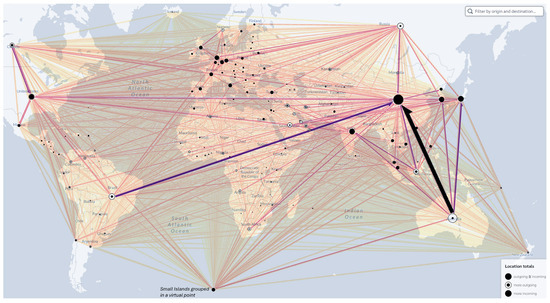
Figure A4.
Bilateral trade flows, measured in tons, for the year 2019.
References
- Torreglosa, J.P.; González-Rivera, E.; García-Triviño, P.; Vera, D. Performance Analysis of a Hybrid Electric Ship by Real-Time Verification. Energies 2022, 15, 2116. [Google Scholar] [CrossRef]
- Motlagh, H. Towards International Maritime Organization carbon targets: A multi-criteria decision-making analysis for sustainable container shipping. Sustainability 2023, 15, 16834. [Google Scholar] [CrossRef]
- Christodoulou, A.; Dalaklis, D.; Ölçer, A.I.; Ballini, F. Can Market-Based Measures Stimulate Investments in Green Technologies for the Abatement of GHG Emissions From Shipping? A Review of Proposed Market-Based Measures. Trans. Marit. Sci. 2021, 10, 208–215. [Google Scholar] [CrossRef]
- Serra, P.; Fancello, G. Towards the IMO’s GHG Goals: A Critical Overview of the Perspectives and Challenges of the Main Options for Decarbonizing International Shipping. Sustainability 2020, 12, 3220. [Google Scholar] [CrossRef]
- Bouman, E.A.; Lindstad, E.; Rialland, A.I.; Strømman, A.H. State-of-the-art technologies, measures, and potential for reducing GHG emissions from shipping—A review. Transp. Res. Part D Transp. Environ. 2017, 52, 408–421. [Google Scholar] [CrossRef]
- Mallouppas, G.; Yfantis, E.A. Decarbonization in Shipping Industry: A Review of Research, Technology Development, and Innovation Proposals. J. Mar. Sci. Eng. 2021, 9, 415. [Google Scholar] [CrossRef]
- Fan, L.; Yang, H.; Zhang, X. Targeting the Effectiveness Assessment of the Emission Control Policies on the Shipping Industry. Sustainability 2024, 16, 2465. [Google Scholar] [CrossRef]
- Christodoulou, A.; Woxenius, J. Sustainable Short Sea Shipping. Sustainability 2019, 11, 2847. [Google Scholar] [CrossRef]
- IMO. Annex 5 of Resolution MEPC.308(73): 2018 Guidelines on the Method of Calculation of the Attained Energy Efficiency Design Index (EEDI) for New Ships; IMO: London, UK, 2018. [Google Scholar]
- IMO. Annex 8 of Resolution MEPC.346(78): 2022 Guidelines for the Development of a Ship Energy Efficiency Management Plan (SEEMP); IMO: London, UK, 2022. [Google Scholar]
- IMO. Annex 12 of Resolution MEPC.350(78): 2022 Guidelines on the Method of Calculation of the Attained Energy Efficiency Existing Ship Index (EEXI); IMO: London, UK, 2022. [Google Scholar]
- IMO. Annex 14 of Resolution MEPC.352(78): 2022 Guidelines on Operational Carbon Intensity Indicators and the Calculation Methods (CII Guidelines, G1); IMO: London, UK, 2022. [Google Scholar]
- Zamboni, G. Comparative analysis among different alternative fuels for ship propulsion in a well-to-wake perspective. Heliyon 2024, 10, e26016. [Google Scholar] [CrossRef]
- Zincir, B.A.; Arslanoglu, Y. Comparative Life Cycle Assessment of Alternative Marine Fuels. Fuel 2024, 358, 129995. [Google Scholar] [CrossRef]
- Lee, H.; Lee, J.; Roh, G.; Lee, S.; Choung, C.; Kang, H. Comparative Life Cycle Assessments and Economic Analyses of Alternative Marine Fuels: Insights for Practical Strategies. Sustainability 2024, 16, 2114. [Google Scholar] [CrossRef]
- Zwaginga, J.; Lagemann, B.; Erikstad, S.O.; Pruyn, J. Optimal Ship Fuel Selection under Life Cycle Uncertainty. Sustainability 2024, 16, 1947. [Google Scholar] [CrossRef]
- Chen, S.; Zheng, S.; Sys, C. Policies focusing on market-based measures towards shipping decarbonization: Designs, impacts and avenues for future research. Transp. Policy 2023, 137, 109–124. [Google Scholar] [CrossRef]
- Marrero, A.; Martínez-López, A. Decarbonization of Short Sea Shipping in European Union: Impact of market and goal based measures. J. Clean. Prod. 2023, 421, 138481. [Google Scholar] [CrossRef]
- Psaraftis, H.N.; Zis, T.; Lagouvardou, S. A comparative evaluation of market based measures for shipping decarbonization. Marit. Transp. Res. 2021, 2, 100019. [Google Scholar] [CrossRef]
- Müller-Casseres, E.; Leblanc, F.; Berg, M.v.d.; Fragkos, P.; Dessens, O.; Naghash, H.; Draeger, R.; Gallic, T.L.; Tagomori, I.S.; Tsiropoulos, I.; et al. International shipping in a world below 2 °C. Nat. Clim. Chang. 2024, 14, 600–607. [Google Scholar] [CrossRef]
- Pereda, P.C.; Lucchesi, A.; Oliveira, T.D.; Wolf, R.; Marques, C.H.; Assis, L.F.; Caprace, J.-D. Sustainable Shipping: Modeling Economic and Greenhouse Gas Impacts of Decarbonization Policies (Part II). Sustainability 2025, 17, 3765. [Google Scholar] [CrossRef]
- Brans, J.; Vincke, P.; Mareschal, B. How to select and how to rank projects: The Promethee method. Eur. J. Oper. Res. 1986, 24, 228–238. [Google Scholar] [CrossRef]
- Horton, G.; Finney, H.; Fischer, S.; Sikora, I.; McQuillen, J.; Ash, N.; Shakeel, H. Technological, Operational and Energy Pathways for Maritime Transport to Reduce Emissions Towards 2050; Report; Ricardo Energy and Environment: Shoreham-by-Sea, UK, 2022. [Google Scholar]
- GLOSTEN. The Ship Operation Cooperative Program-Energy Efficiency Report; Report; Glosten: Seattle, WA, USA, 2016. [Google Scholar]
- ABS. Ship Energy Efficiency Measures-Status and Guidance; Report; American Bureau of Shipping (ABS): Houston, TX, USA, 2013. [Google Scholar]
- Halim, R.; Kirstein, L.; Merk, O.; Martinez, L. Decarbonization Pathways for International Maritime Transport: A Model-Based Policy Impact Assessment. Sustainability 2018, 10, 2243. [Google Scholar] [CrossRef]
- Tunagur, E. ‘Low Maturity of Solutions’ the Main Barrier to Decarbonisation, Lloyd’s List Survey Finds; Lloyd’s Register: London, UK, 2023. [Google Scholar]
- Akula, N. Adopting a Business Model Approach for Developing a Ship Design Strategy to Optimise Life Cycle Costs and Emissions by ReDesigning for Circular Economy. Ph.D. Thesis, Université De Liège, Liège, Belgium, 2023. [Google Scholar]
- Jeong, H.; Yun, H. A stochastic approach for economic valuation of alternative fuels: The case of container ship investments. J. Clean. Prod. 2023, 418, 138182. [Google Scholar] [CrossRef]
- Maersk. Preparing Container Vessels for Conversion to Green Fuels; Report; Maersk: Copenhagen, Denmark, 2022. [Google Scholar]
- Casseres, E.M.M.D. Potencial De Mitigação Das Emissões De CO2 Do Transporte Marítimo Internacional: Uma Analise Baseada Em Cenários Para O Caso Dos Navios-Tanque De Petróleo Bruto. Ph.D. Thesis, Universidade Federal do Rio de Janeiro-UFRJ, Rio de Janeiro, Brazil, 2018. [Google Scholar]
- Stavroulakis, P.J.; Papadimitriou, S. Total cost of ownership in shipping: A framework for sustainability. J. Shipp. Trade 2022, 7, 14. [Google Scholar] [CrossRef]
- Global Trade Analysis Project (GTAP). GTAP Detailed Sectoral Contributions. 2025. Available online: https://www.gtap.agecon.purdue.edu/databases/contribute/detailedsector.asp (accessed on 30 January 2025).
- Pereda, P.; Lucchesi, A.; Oliveira, T.D.; Wolf, R. Carbon Tax in the Shipping Sector: Assessing Economic and Environmental Impacts. SSRN 2023. [Google Scholar] [CrossRef]
- International Institute for Applied Systems Analysis (IIASA). Shared Socioeconomic Pathways (SSP) Database. 2024. Available online: https://iiasa.ac.at/models-tools-data/ssp (accessed on 10 January 2024).
- IMO. Resolution Mepc.391(81)–2024 Guidelines on Life Cycle GHG Intensity of Marine Fuels (2024 Lca Guidelines); IMO: London, UK, 2024. [Google Scholar]
- IMO. MEPC82-INF-8-Add-1–Report of the Comprehensive Impact Assessment of the Basket of Candidate GHG Reduction Mid-Term Measures–Full Report on Task 2 (Impacts on the Fleet)–Conducted by: DNV; IMO: London, UK, 2024. [Google Scholar]
- IMO. Annex 1 of Resolution MEPC.328(76): Amendments to the Annex of the Protocol of 1997 to Amend the International Convention for the Prevention of Pollution from Ships, 1973, as Modified by the Protocol of 1978 Relating Thereto; IMO: London, UK, 2021. [Google Scholar]
- IMO. Annex 16 of Resolution MEPC.322(74): Amendments to the 2018 Guidelines on the Method of Calculation of the Attained Energy Efficiency Design Index (EEDI) for New Ships (Resolution MEPC.208(73)); IMO: London, UK, 2019. [Google Scholar]
- Marques, C.H.; Pereda, P.C.; Lucchesi, A.; Ramos, R.F.; Fiksdahl, O.; Assis, L.F.; Pereira, N.N.; Caprace, J.D. Cost and environmental impact assessment of mandatory speed reduction of maritime fleets. Mar. Policy 2023, 147, 105334. [Google Scholar] [CrossRef]
- IMO. Annex 15 of Resolution MEPC.353(78): 2022 Guidelines on the Reference Lines for Use with Operational Carbon Intensity Indicators (CII Reference Lines Guidelines, G2); IMO: London, UK, 2022. [Google Scholar]
- IMO. Annex 16 of Resolution MEPC.354(78): 2022 Guidelines on the Operational Carbon Intensity Rating of Ships (CII Rating Guidelines, G4); IMO: London, UK, 2022. [Google Scholar]
- Geels, F.W. The multi-level perspective on sustainability transitions: Responses to seven criticisms. Environ. Innov. Soc. Transit. 2011, 1, 24–40. [Google Scholar] [CrossRef]
- Psaraftis, H.N.; Kontovas, C.A. Decarbonization of Maritime Transport: Is There Light at the End of the Tunnel? Sustainability 2021, 13, 237. [Google Scholar] [CrossRef]
- IMO. MEPC 76-7-12–Proposal for IMO to Establish a Universal Mandatory Greenhouse Gas Levy–Submitted by: Marshall Islands and Solomon Islands; Report; IMO: London, UK, 2021. [Google Scholar]
- IMO. MEPC 77-7-4–Proposed Draft Amendments to MARPOL Annex VI–Submitted by: Marshall Islands and Solomon Islands; Report; IMO: London, UK, 2021. [Google Scholar]
- Fund, G.C. Annex I: Audited Financial Statements of the Green Climate Fund for the Year Ended 31 December 2019; Technical Report; GCF: Incheon, Republic of Korea, 2019. [Google Scholar]
- IMO. ISWG-GHG 13-4-6–Refined Proposal on Zero-Emission Shipping Incentive Scheme (ZESIS) to Incentivize GHG Emission Reduction and to Make an Equitable Transition–Submitted by: Japan; Report; IMO: London, UK, 2022. [Google Scholar]
- IMO. ISWG-GHG 14-3-1–Further Proposal on Zero-Emission Shipping Incentive Scheme (ZESIS)–Submitted by: Japan; Report; IMO: London, UK, 2021. [Google Scholar]
- IMO. ISWG-GHG 16-2-12–Further Proposal on the Feebate Mechanism–Submitted by: Japan; Journal Article IMO ISWG-GHG 16-2-12; IMO: London, UK, 2024. [Google Scholar]
- IMO. ISWG-GHG 16-2-10—The Need for Flexibility in the Greenhouse Gas Fuel Standard (GFS) and Criteria That a Flexibility Mechanism Should Meet–Submitted by: Austria, Belgium, Bulgaria, Croatia, Cyprus, Czechia, Denmark, Estonia, Finland, France, Germany, Greece, Hungary, Ireland, Italy, Latvia, Lithuania, Luxembourg, Malta, Netherlands, Poland, Portugal, Romania, Slovakia, Slovenia, Spain, Sweden and EC; IMO: London, UK, 2024. [Google Scholar]
- IMO. ISWG-GHG 16-2-13–Further Proposal on the International Maritime Sustainable Fuels and Fund (IMSF&F) Mechanism and Associated Draft Amendments to MARPOL Annex VI–Submitted by: Brazil, China, Norway and UAE; IMO: London, UK, 2024. [Google Scholar]
- IMO. ISWG-GHG 16-2-14–Elaborations on the Key Elements of the International Maritime Sustainable Fuels and Fund (IMSF&F) Mechanism Presented in Document ISWG-GHG 16/2/13–Submitted by: Brazil, China, Norway and UAE; IMO: London, UK, 2024. [Google Scholar]
- Norwegian Ministry of Climate and Environment. GFI and Economic Element; Technical report; Working Paper of the Norwegian Ministry of Climate and Environment; Norwegian Ministry of Climate and Environment: Oslo, Norway, 2024. [Google Scholar]
- Uchôa, I.M.; Deus, M.S.; Barros Neto, E.L. Formulation and tribological behavior of ultra-low sulfur diesel fuels microemulsified with glycerin. Fuel 2021, 292, 120257. [Google Scholar] [CrossRef]
- Uyar, M.; Aydın, H. Production of low sulfur diesel-like fuel from crude oil wastes by pyrolytic distillation and its usage in a diesel engine. Energy 2022, 244, 122683. [Google Scholar] [CrossRef]
- Vedachalam, S.; Dalai, A.K. Hydrotreating and oxidative desulfurization of heavy fuel oil into low sulfur marine fuel over dual function NiMo/γ–Al2O3 catalyst. Catal. Today 2023, 407, 165–171. [Google Scholar] [CrossRef]
- Zhang, Y.Y.; Zhang, Y.J. The impact of institutional analyst forecast divergence on crude oil market: Evidence from the mixed frequency models. Int. Rev. Financ. Anal. 2022, 84, 102418. [Google Scholar] [CrossRef]
- Meza, A.; Koç, M.; Al-Sada, M.S. Perspectives and strategies for LNG expansion in Qatar: A SWOT analysis. Resour. Policy 2022, 76, 102633. [Google Scholar] [CrossRef]
- Elgohary, M.M.; Seddiek, I.S.; Salem, A.M. Overview of alternative fuels with emphasis on the potential of liquefied natural gas as future marine fuel. Proc. Inst. Mech. Eng. Part M J. Eng. Marit. Environ. 2014, 229, 365–375. [Google Scholar] [CrossRef]
- Winnes, H.; Fridell, E.; Hansson, J.; Jivén, K. Biofuels for Low Carbon Shipping; IVL Swedish Environmental Research Institute: Stockholm, Sweden, 2019. [Google Scholar]
- Carvalho, F.; Müller-Casseres, E.; Poggio, M.; Nogueira, T.; Fonte, C.; Wei, H.K.; Portugal-Pereira, J.; Rochedo, P.R.; Szklo, A.; Schaeffer, R. Prospects for carbon-neutral maritime fuels production in Brazil. J. Clean. Prod. 2021, 326, 129385. [Google Scholar] [CrossRef]
- Wei, H.K. Análise Comparativa do Porto ao Navio de Combustíveis Alternativos Para Transporte Marítimo. Master’s Thesis, Universidade Federal do Rio de Janeiro (UFRJ), Rio de Janeiro, Brazil, 2021. [Google Scholar]
- Tijmensen, M.J.; Faaij, A.P.; Hamelinck, C.N.; van Hardeveld, M.R. Exploration of the possibilities for production of Fischer Tropsch liquids and power via biomass gasification. Biomass Bioenergy 2002, 23, 129–152. [Google Scholar] [CrossRef]
- Van Uy, D.; The Nam, T. Fuel Continuous Mixer—An Approach Solution to Use Straight Vegetable Oil for Marine Diesel Engines. TransNav Int. J. Mar. Navig. Saf. Sea Transp. 2018, 12, 151–157. [Google Scholar] [CrossRef]
- Commission, E.; Centre, J.R.; Padella, M.; O’Connell, A.; Giuntoli, J.; Bulgheroni, C.; Edwards, R.; Marelli, L.; Koeble, R. Definition of Input Data to Assess GHG Default Emissions from Biofuels in EU Legislation–Version 1d-2019; Publications Office: Brussels, Belgium, 2019. [Google Scholar] [CrossRef]
- Radonja, R.; Bebić, D.; Glujić, D. Methanol and Ethanol as Alternative Fuels for Shipping. Promet-Traffic Transp. 2019, 31, 321–327. [Google Scholar] [CrossRef]
- Joanne Ellis, K. Study on the Use of Ethyl and Methyl Alcohol as Alternative Fuels in Shipping; Technical report; European Maritime Safety Agency: Lisbon, Portugal, 2015. [Google Scholar]
- Yang, S.; Feng, J.; Sun, P.; Wang, Y.; Dong, W.; Yu, X.; Li, W. Combustion and emissions characteristics of methanol/gasoline CISI engines under different injection modes. Fuel 2023, 333, 126506. [Google Scholar] [CrossRef]
- Dagmar, N. Availability and Costs of Liquefied Bio- and Synthetic Methane; CE Delft: Delft, The Netherlands, 2020. [Google Scholar]
- Hansson, J.; Brynolf, S.; Fridell, E.; Lehtveer, M. The Potential Role of Ammonia as Marine Fuel—Based on Energy Systems Modeling and Multi-Criteria Decision Analysis. Sustainability 2020, 12, 3265. [Google Scholar] [CrossRef]
- Abubakar Mahmud Sheriff, A.T. Assessment of Ammonia Ignition as a Maritime Fuel, Using Engine Experiments and Chemical Kinetic Simulations. Master’s Thesis, World Maritime University, Malmö, Sweden, 2019. [Google Scholar]
- Vries, N.d. Safe and Effective Application of Ammonia as a Marine Fuel. Master’s Thesis, Delft University of Technology, Delft, The Netherlands, 2019. [Google Scholar]
- MAN. Engineering the Future Two-Stroke Green-Ammonia Engine; MAN: Copenhagen, Denmark, 2019. [Google Scholar]
- Dimitriou, P.; Tsujimura, T. A review of hydrogen as a compression ignition engine fuel. Int. J. Hydrogen Energy 2017, 42, 24470–24486. [Google Scholar] [CrossRef]
- Babayev, R.; Andersson, A.; Serra Dalmau, A.; Im, H.G.; Johansson, B. Computational comparison of the conventional diesel and hydrogen direct-injection compression-ignition combustion engines. Fuel 2022, 307, 121909. [Google Scholar] [CrossRef]
- Babayev, R.; Im, H.G.; Andersson, A.; Johansson, B. Hydrogen double compression-expansion engine (H2DCEE): A sustainable internal combustion engine with 60%+ brake thermal efficiency potential at 45 bar BMEP. Energy Convers. Manag. 2022, 264, 115698. [Google Scholar] [CrossRef]
- Boretti, A. Hydrogen internal combustion engines to 2030. Int. J. Hydrogen Energy 2020, 45, 23692–23703. [Google Scholar] [CrossRef]
- Aggarwal, A.; Yadav, S.; Singh, K.; Singh Verma, A.; Chhabra, S. Study of utilization of hydrogen as fuel in internal combustion engine. Mater. Today Proc. 2022, 64, 1211–1216. [Google Scholar] [CrossRef]
- Lungu, A. Energy-Saving Devices in Ship Propulsion: Effects of Nozzles Placed in Front of Propellers. J. Mar. Sci. Eng. 2021, 9, 125. [Google Scholar] [CrossRef]
- Mewis, F. Six Years Mewis Duct-Six Years of Hydrodynamic Development. In Proceedings of the Sprechtag FA SchiffsHydrodynamik; Schiffahrts-Verlag Hansa GmbH & Co. KG.: Hamburg, Germany, 2014. [Google Scholar]
- Gaggero, S.; Martinelli, M. Pre-swirl fins design for improved propulsive performances: Application to fast twin-screw passenger ships. J. Ocean Eng. Mar. Energy 2022, 9, 69–91. [Google Scholar] [CrossRef]
- Koushan, K.; Krasilnikov, V.; Nataletti, M.; Sileo, L.; Spence, S. Experimental and Numerical Study of Pre-Swirl Stators PSS. J. Mar. Sci. Eng. 2020, 8, 47. [Google Scholar] [CrossRef]
- Kim, J.H.; Choi, J.E.; Choi, B.J.; Chung, S.H.; Seo, H.W. Development of energy-saving devices for a full slow-speed ship through improving propulsion performance. Int. J. Nav. Archit. Ocean Eng. 2015, 7, 390–398. [Google Scholar] [CrossRef]
- Lim, S.S.; Kim, T.W.; Lee, D.M.; Kang, C.G.; Kim, S.Y. Parametric study of propeller boss cap fins for container ships. Int. J. Nav. Archit. Ocean Eng. 2014, 6, 187–205. [Google Scholar] [CrossRef]
- Sankpal, S.D.; Bm, D.S. CFD Analysis on Propeller Performance with Propeller Boss Cap Fin. Int. J. Recent Technol. Eng. (IJRTE) 2019, 8, 9516–9521. [Google Scholar] [CrossRef]
- Yao, Z.Q.; Gu, X.; Shen, Y. The Research of Hydrodynamic Performance for Ducted Propeller with PBCF. Appl. Mech. Mater. 2015, 733, 578–582. [Google Scholar] [CrossRef]
- Sukas, O.F.; Kinaci, O.K.; Bal, S. Asymmetric ship maneuvering due to twisted rudder using system-based and direct CFD approaches. Appl. Ocean Res. 2021, 108, 102529. [Google Scholar] [CrossRef]
- Sasaki, N.; Atlar, M.; Kuribayashi, S. Advantages of twin rudder system with asymmetric wing section aside a propeller. J. Mar. Sci. Technol. 2016, 21, 297–308. [Google Scholar] [CrossRef]
- Efremov, D. Determining the Asymmetric Rudder Efficiency of a Twin Rudder Patrol Ship at Manoeuvring. Eng. Sci. 2021, LVIII, 24–44. [Google Scholar] [CrossRef]
- Gaggero, S.; Martinelli, M. Pre- and post-swirl fins design for improved propulsive performances. Ship Technol. Res. 2022, 69, 31–49. [Google Scholar] [CrossRef]
- Elangovan, M. Hydrodynamic Energy Devices to Improve the Efficiency of Propulsion System in AUVs. Int. Res. J. Adv. Sci. Hub 2020, 2, 18–22. [Google Scholar] [CrossRef]
- Villa, D.; Gaggero, S.; Tani, G.; Viviani, M. Numerical and Experimental Comparison of Ducted and Non-Ducted Propellers. J. Mar. Sci. Eng. 2020, 8, 257. [Google Scholar] [CrossRef]
- Cai, B.; Mao, X.; Xu, Q.; Chai, W.; Tian, B.; Qiu, L. Simulation of the interaction between ship and ducted propeller with a modified body force method. Ocean Eng. 2022, 249, 110950. [Google Scholar] [CrossRef]
- Kim, S.; Kinnas, S.A. A panel method for the prediction of unsteady performance of ducted propellers in ship behind condition. Ocean Eng. 2022, 246, 110582. [Google Scholar] [CrossRef]
- Sánchez-Caja, A.; González-Adalid, J.; Pérez-Sobrino, M.; Saisto, I. Study of end-plate shape variations for tip loaded propellers using a RANSE solver. In Proceedings of the 29th Symposium on Naval Hydrodynamics, Gothenburg, Sweden, 26–31 August 2012; pp. 26–31. [Google Scholar]
- Kang, J.G.; Kim, M.C.; Kim, H.U.; Shin, I.R. Study on Propulsion Performance by Varying Rake Distribution at the Propeller Tip. J. Mar. Sci. Eng. 2019, 7, 386. [Google Scholar] [CrossRef]
- Tadros, M.; Ventura, M.; Guedes Soares, C. Towards Fuel Consumption Reduction Based on the Optimum Contra-Rotating Propeller. J. Mar. Sci. Eng. 2022, 10, 1657. [Google Scholar] [CrossRef]
- Zhu, W.; Zhou, F.; Shu, H.; Hu, G. Effect of contra-rotating propeller boss cap fins (CRPBCF) on the performance of marine propellers. Ocean Eng. 2022, 266, 112932. [Google Scholar] [CrossRef]
- Hou, L.; Yin, L.; Hu, A.; Chang, X.; Lin, Y.; Wang, S. Optimal matching investigation of marine contra-rotating propellers for energy consumption minimization. J. Mar. Sci. Technol. 2021, 26, 1184–1197. [Google Scholar] [CrossRef]
- Wang, Z.Z.; Min, S.S.; Peng, F.; Shen, X.R. Comparison of self-propulsion performance between vessels with single-screw propulsion and hybrid contra-rotating podded propulsion. Ocean Eng. 2021, 232, 109095. [Google Scholar] [CrossRef]
- Pavlov, G.A.; Yun, L.; Bliault, A.; He, S.L. Air Lubricated and Air Cavity Ships; Springer: Berlin/Heidelberg, Germany, 2020. [Google Scholar] [CrossRef]
- Fotopoulos, A.G.; Margaris, D.P. Computational Analysis of Air Lubrication System for Commercial Shipping and Impacts on Fuel Consumption. Computation 2020, 8, 38. [Google Scholar] [CrossRef]
- An, H.; Pan, H.; Yang, P. Research Progress of Air Lubrication Drag Reduction Technology for Ships. Fluids 2022, 7, 319. [Google Scholar] [CrossRef]
- Giernalczyk, M.; Kaminski, P. Assessment of the Propulsion System Operation of the Ships Equipped with the Air Lubrication System. Sensors 2021, 21, 1357. [Google Scholar] [CrossRef] [PubMed]
- Bispo, R.L.P.; Souza, J.A.; Caprace, J.D.; Ordonez, J.C.; Marques, C.H. A Parametric Study on Air Lubrication for Ship Energy Efficiency. J. Mar. Sci. Eng. 2024, 12, 2309. [Google Scholar] [CrossRef]
- Mohammadpour, J.; Salehi, F.; Garaniya, V.; Baalisampang, T.; Arzaghi, E.; Roberts, R.; Cervella, G.; Newport, J.; Hughes, P.; Abbassi, R. Computational analysis of air bubble-induced frictional drag reduction on ship hulls. J. Mar. Sci. Technol. 2024, 29, 696–710. [Google Scholar] [CrossRef]
- Ma, M.; Qi, Y.; Zhang, C.; Chen, Q.; Gu, C.; Zhang, Z. Highly efficient antifouling and toughening hydrogel for ship coatings. Appl. Surf. Sci. 2024, 662, 160102. [Google Scholar] [CrossRef]
- Wu, Y.; Hua, J.; Wu, D. Economic analysis of ship operation using a new antifouling strategy. Ocean Eng. 2022, 266, 113038. [Google Scholar] [CrossRef]
- Kumar, S.; Verma, K.A.; Pandey, K.M.; Sharma, K.K. A review on methods used to reduce drag of the ship hulls to improve hydrodynamic characteristics. Int. J. Hydromechatronics 2020, 3, 297–312. [Google Scholar] [CrossRef]
- Qin, L.; Lu, S.; Liu, J.; Wu, Y.; Ma, Z.; Mawignon, F.J.; Dong, G. Bionic non-smooth epoxy resin coating with corrosion inhibitor for drag-reduction and durability. Prog. Org. Coat. 2022, 173, 107176. [Google Scholar] [CrossRef]
- Cao, Z.; Cao, P. Research Progress on Low-Surface-Energy Antifouling Coatings for Ship Hulls: A Review. Biomimetics 2023, 8, 502. [Google Scholar] [CrossRef]
- MAN Diesel & Turbo. Shaft Generators for the MC and ME Engines; MAN Diesel & Turbo: Copenhagen, Denmark, 2012. [Google Scholar]
- MAN Energy Solutions. Shaft Generators for Low Speed Main Engines; MAN Energy Solutions: Augsburg, Germany, 2021. [Google Scholar]
- Traut, M.; Gilbert, P.; Walsh, C.; Bows, A.; Filippone, A.; Stansby, P.; Wood, R. Propulsive power contribution of a kite and a Flettner rotor on selected shipping routes. Appl. Energy 2014, 113, 362–372. [Google Scholar] [CrossRef]
- Ballini, F.; Ölçer, A.I.; Brandt, J.; Neumann, D. Health costs and economic impact of wind assisted ship propulsion. Ocean Eng. 2017, 146, 477–485. [Google Scholar] [CrossRef]
- Li, B.; Zhang, R.; Zhang, B.; Yang, Q.; Guo, C. An assisted propulsion device of vessel utilizing wind energy based on Magnus effect. Appl. Ocean Res. 2021, 114, 102788. [Google Scholar] [CrossRef]
- Tillig, F.; Ringsberg, J.W.; Psaraftis, H.N.; Zis, T. Reduced environmental impact of marine transport through speed reduction and wind assisted propulsion. Transp. Res. Part D Transp. Environ. 2020, 83, 102380. [Google Scholar] [CrossRef]
- Tillig, F.; Ringsberg, J.W. Design, operation and analysis of wind-assisted cargo ships. Ocean Eng. 2020, 211, 107603. [Google Scholar] [CrossRef]
- Bordogna, G.; Muggiasca, S.; Giappino, S.; Belloli, M.; Keuning, J.A.; Huijsmans, R.H.M.; Van ’T Veer, A.P. Experiments on a Flettner rotor at critical and supercritical Reynolds numbers. J. Wind. Eng. Ind. Aerodyn. 2019, 188, 19–29. [Google Scholar] [CrossRef]
- Talluri, L.; Nalianda, D.K.; Giuliani, E. Techno economic and environmental assessment of Flettner rotors for marine propulsion. Ocean Eng. 2018, 154, 1–15. [Google Scholar] [CrossRef]
- Rehmatulla, N.; Parker, S.; Smith, T.; Stulgis, V. Wind technologies: Opportunities and barriers to a low carbon shipping industry. Mar. Policy 2017, 75, 217–226. [Google Scholar] [CrossRef]
- Silva, M.F.; Friebe, A.; Malheiro, B.; Guedes, P.; Ferreira, P.; Waller, M. Rigid wing sailboats: A state of the art survey. Ocean Eng. 2019, 187, 106150. [Google Scholar] [CrossRef]
- Bot, P.; Viola, I.M.; Flay, R.G.J.; Brett, J.S. Wind-tunnel pressure measurements on model-scale rigid downwind sails. Ocean Eng. 2014, 90, 84–92. [Google Scholar] [CrossRef]
- Marques, C.H.; Caprace, J.D.; Belchior, C.R.P.; Martini, A. An Approach for Predicting the Specific Fuel Consumption of Dual-Fuel Two-Stroke Marine Engines. J. Mar. Sci. Eng. 2019, 7, 20. [Google Scholar] [CrossRef]
- Silva, A.R.d.; França, G.C.; Ordonez, J.C.; Marques, C.H. Fuel Consumption Prediction in Dual-Fuel Low-Speed Marine Engines With Low-Pressure Gas Injection. J. Energy Resour. Technol. 2024, 146, 122103. [Google Scholar] [CrossRef]
- Smith, T. The Cost of Reducing Greenhouse Gas Emissions in Shipping; International Transport Forum: Paris, France, 2020. [Google Scholar] [CrossRef]
- Jupe, M. The Management of Ships; Report; Drewry Shipping Consultants Ltd.: London, UK, 2009. [Google Scholar]
- Stopford, M. Maritime Economics; Routledge: London, UK, 2009. [Google Scholar]
- Deniz, C.; Zincir, B. Environmental and economical assessment of alternative marine fuels. J. Clean. Prod. 2016, 113, 438–449. [Google Scholar] [CrossRef]
- Perčić, M.; Vladimir, N.; Fan, A. Life-cycle cost assessment of alternative marine fuels to reduce the carbon footprint in short-sea shipping: A case study of Croatia. Appl. Energy 2020, 279, 115848. [Google Scholar] [CrossRef]
- Ashrafi, M.; Lister, J.; Gillen, D. Toward a harmonization of sustainability criteria for alternative marine fuels. Marit. Transp. Res. 2022, 3, 100052. [Google Scholar] [CrossRef]
- Lagemann, B.; Lindstad, E.; Fagerholt, K.; Rialland, A.; Ove Erikstad, S. Optimal ship lifetime fuel and power system selection. Transp. Res. Part D Transp. Environ. 2022, 102, 103145. [Google Scholar] [CrossRef]
- Psaraftis, H.N.; Kontovas, C.A. Speed models for energy-efficient maritime transportation: A taxonomy and survey. Transp. Res. Part C Emerg. Technol. 2013, 26, 331–351. [Google Scholar] [CrossRef]
- Mallidis, I.; Iakovou, E.; Dekker, R.; Vlachos, D. The impact of slow steaming on the carriers’ and shippers’ costs: The case of a global logistics network. Transp. Res. Part E Logist. Transp. Rev. 2018, 111, 18–39. [Google Scholar] [CrossRef]
- Tomazos, F. Shipbuilding Trends. Impact Fleet Renewal & Fuel Landscape; Cass Tecnava Maritime: Palaio Faliro, Greece, 2023. [Google Scholar]
- Wang, Y.; Wright, L.A. A Comparative Review of Alternative Fuels for the Maritime Sector: Economic, Technology, and Policy Challenges for Clean Energy Implementation. World 2021, 2, 456–481. [Google Scholar] [CrossRef]
- Seddiek, I.S.; Ammar, N.R. Technical and eco-environmental analysis of blue/green ammonia-fueled RO/RO ships. Transp. Res. Part D Transp. Environ. 2023, 114, 103547. [Google Scholar] [CrossRef]
- Kowalak, P. Chief engineer’s hands-on experience of slow steaming operation. 2013. [Google Scholar] [CrossRef]
- Woud, H.; Stapersma, D. Design of Propulsion and Electric Power Generation Systems; IMarEST, Institute of Marine Engineering, Science and Technology: Singapore, 2002. [Google Scholar]
- Ryste, J.A. Comparison of Alternative Marine Fuels; Report; DNV-GL: Bærum, Norway, 2019. [Google Scholar]
- Hansson, J.; Månsson, S.; Brynolf, S.; Grahn, M. Alternative marine fuels: Prospects based on multi-criteria decision analysis involving Swedish stakeholders. Biomass Bioenergy 2019, 126, 159–173. [Google Scholar] [CrossRef]
- Cullinane, K.; Yang, J. Evaluating the Costs of Decarbonizing the Shipping Industry: A Review of the Literature. J. Mar. Sci. Eng. 2022, 10, 946. [Google Scholar] [CrossRef]
- Solakivi, T.; Paimander, A.; Ojala, L. Cost competitiveness of alternative maritime fuels in the new regulatory framework. Transp. Res. Part D Transp. Environ. 2022, 113, 103500. [Google Scholar] [CrossRef]
- Brans, J.P.; Mareschal, B. Promethee Methods. In Multiple Criteria Decision Analysis: State of the Art Surveys; Springer: New York, NY, USA, 2005; pp. 163–186. [Google Scholar] [CrossRef]
Disclaimer/Publisher’s Note: The statements, opinions and data contained in all publications are solely those of the individual author(s) and contributor(s) and not of MDPI and/or the editor(s). MDPI and/or the editor(s) disclaim responsibility for any injury to people or property resulting from any ideas, methods, instructions or products referred to in the content. |
© 2025 by the authors. Licensee MDPI, Basel, Switzerland. This article is an open access article distributed under the terms and conditions of the Creative Commons Attribution (CC BY) license (https://creativecommons.org/licenses/by/4.0/).