Abstract
Glaciers are one of the most important water resources in the arid regions of Xinjiang, making it crucial to accurately monitor glacier changes for the region’s sustainable development. However, due to their typical distribution in remote, high-altitude areas, large-scale and long-term field observations are often constrained by the high costs of manpower, resources, and finances. Globally, fewer than 40 glaciers have been monitored for more than 20 years, and, in China, only Glacier No. 1 at the headwaters of the Urumqi River has monitoring records exceeding 50 years. To address these challenges, this study analyzed glacier changes in the Tomur Peak region of the Tianshan Mountains over the past 35 years using Landsat satellite imagery. Through experiments with deep learning models, the results show that the 3-4-5 band combination performed best for glacier boundary extraction. The DeepLabV3+ model, with MobileNetV2 as the backbone, achieved an overall accuracy of 90.44%, a recall rate of 82.75%, and a mean Intersection over Union (IoU) that was 1.6 to 5.94 percentage points higher than other models. Based on these findings, the study further analyzed glacier changes in the Tomur Peak region, revealing an average annual glacier reduction rate of 0.18% and a retreat rate of 6.97 km2·a−1 over the past 35 years. This research provides a more precise and comprehensive scientific reference for understanding glacier changes in arid regions, with significant implications for enhancing our understanding of the impacts of climate change on glaciers, optimizing water resource management, and promoting regional sustainable development.
1. Introduction
The cryosphere represents the portion of Earth’s surface where water exists in a solid state. Among its components are glaciers, which are recognized as key indicators of global climate change due to their high sensitivity to temperature variations [1,2,3]. Glaciers also constitute one of the most critical freshwater resources worldwide, covering approximately 14.51 × km2 and storing an estimated 27.6 × km³ of water, which accounts for more than 75% of the Earth’s freshwater reserves [4]. However, with the intensification of global warming, the Tianshan region, known for its glaciers’ high sensitivity to climate fluctuations in Central Asia, has witnessed accelerated glacier retreat in most areas since 1900 [5,6,7,8,9,10]. This trend has profound implications for water resource availability [11], sea-level rise [12], and the increased occurrence of natural disasters such as ice avalanches [13,14] and glacial lake outburst floods (GLOFs) [15,16]. Consequently, accurately and efficiently delineating glacier boundaries and monitoring their changes are critical for regional development and disaster mitigation.
Traditional methods for glacier boundary extraction are primarily based on pixel-based classification algorithms, such as Maximum Likelihood Classification (MLC), Support Vector Machine (SVM), and Random Forest (RF). These methods rely on spectral and textural information for classification but are prone to issues like “same object, different spectra”, “same spectra, different objects”, and salt-and-pepper noise. Object-Based Image Analysis (OBIA) approaches, while addressing some of these issues, require the manual adjustment of segmentation parameters, making them less effective in dealing with the spatial complexity of debris-covered glaciers and lacking contextual guidance capabilities [17,18].
Landsat TM/ETM+ imagery, with its moderate spatial resolution and multispectral capabilities, has become a key data source for glacier monitoring and boundary extraction. In particular, studies in the Tomur Peak region have highlighted the value of Landsat data for capturing glacier dynamics. Zhou et al. [19] analyzed multi-temporal Landsat imagery and reported a consistent glacier retreat trend of approximately 4.0% per decade over the past 35 years. Methodologically, the TM4/TM5 band ratio has been shown to offer higher accuracy in delineating pure glacier boundaries [20], while the TM3/TM5 ratio performs better in shadowed regions [21]. Beyond regional case studies, Landsat data have been widely utilized for the long-term monitoring of glacier retreat and snowmelt across various geographic settings. For instance, Paul et al. [22] used Landsat ETM+ imagery to assess glacier changes in northern Norway and the Alps, while Pritam et al. [23] combined Landsat ETM+ and ASTER GDEM data to investigate glacier evolution in the Ravi Basin of the northwestern Himalayas from 1971 to 2013. These studies collectively demonstrate the broad applicability and scientific value of Landsat imagery in global glacier remote sensing.
In recent years, deep learning has shown great promise in geospatial information extraction, particularly in glacier mapping. The introduction of Fully Convolutional Networks (FCNs) by Shelhamer et al. [24] enhanced spatial feature extraction and boosted the performance of semantic segmentation models. Integrating deep learning with Landsat imagery, researchers have advanced glacier mapping. Mohajerani et al. [25] used U-Net to segment Greenland calving fronts but faced limitations due to small input sizes. Davari et al. [26] addressed this by reformulating the task as pixel-wise regression, improving the Dice coefficient by 21%. Xie et al. [27] developed GlacierNet, combining Landsat-8 OLI and terrain data to improve debris-covered glacier recognition. Compared with DeepLabv3+, GlacierNet offered lightweight advantages for constrained settings. To overcome shadow and cloud interference, Wang et al. [28] introduced a context-aware segmentation model, achieving an F1 score of 0.8665. Zhang et al. [29] proposed U-PSP-Net, using pyramid pooling for multi-scale feature extraction, achieving 95.84% accuracy across diverse mountain regions.
Many domestic and international studies have verified the reliability of Landsat data in glacier monitoring and provided mature processing methods. Therefore, in this study, Landsat TM/ETM+ imagery is used for long-term, large-scale monitoring to comprehensively assess glacier change characteristics, given the limitations of traditional glacier boundary extraction algorithms in terms of automation and the lag in information updates. The study found that using RGB composite images to enhance the visual contrast of glacier boundaries improved boundary separation and recognition accuracy. Additionally, the effectiveness of the Band 3, Band 4, and Band 5 band combinations for glacier identification was further validated.
2. Study Area and Data
2.1. Overview of the Study Area
The Tomur Peak region in the western Tianshan Mountains (41°–42° N, 78°–81° E) lies at the intersection of China, Kyrgyzstan, and Kazakhstan, extending in a northwest–southeast direction (Figure 1). It is one of China’s largest areas of modern glacial activity, containing a total of 829 glaciers, 509 of which are located within China’s territory, covering a total area of 2746 square kilometers. A distinctive type of valley glacier, known as branching valley glaciers, is widely distributed throughout the Tomur Peak region. These glaciers exhibit particularly notable features, including the widespread presence of multi-tongued structures, dense debris cover on glacier surfaces, and well-developed thermokarst landforms. Based on these unique glacial characteristics, researchers classify the glaciers in this region as “Tomur-type” glaciers.
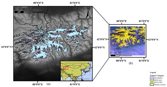
Figure 1.
(a) The location of the Tomur Peak glacier region. (b) The false-color Landsat remote sensing image.
2.2. Data Sources
2.2.1. Satellite Data
This study selected Landsat TM/ETM+ satellite imagery covering the Tomur Peak region (detailed in Table 1), with data sourced from the USGS Earth Explorer platform (https://earthexplorer.usgs.gov, accessed on 15 May 2024). The downloaded images are Top-of-Atmosphere (TOA) reflectance products. To enhance the accuracy of glacier boundary extraction, priority was given to images acquired during the glacier ablation season with minimal cloud cover. The 16-day revisit cycle of Landsat satellites provides high temporal resolution, significantly increasing the availability of suitable imagery. A total of 18 scenes were selected for analysis, each with a spatial resolution of approximately 8200 × 7200 pixels, covering a 35-year time span.

Table 1.
Details of Landsat series satellite data used from 1989 to 2023.
2.2.2. Reference Data
The glacier boundary labels were derived from the RGI6.0 (Randolph Glacier Inventory) glacier boundary vector files provided by the Global Land Ice Measurements from Space (GLIMS) project. Glacier lake labels were obtained from the 2015 Glacier Lake Catalog of Western China, available from the Scientific Data Bank (https://www.scidb.cn, accessed on 20 May 2024), which contains detailed information on the distribution, area, and number of glacier lakes in the region. In this study, glacier lake vector files and glacier boundary vector files corresponding to the Tomur Peak region were selected as annotation references for the convolutional neural network, providing a solid foundation to ensure the scientific rigor and accuracy of data labeling.
3. Materials and Methods
The technical workflow is shown in Figure 2. Initially, the Landsat satellite imagery is preprocessed, and a dataset is constructed. Subsequently, a comparative experiment with various semantic segmentation models is conducted, and the model with the best classification performance is selected to ensure the accuracy of the glacier classification results. Thereafter, the glacier extraction model is applied to classify three land cover types in the Tomur Peak region from 1989 to 2023, followed by a change analysis.
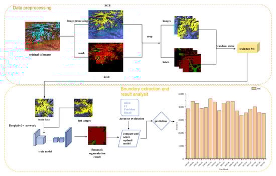
Figure 2.
Flowchart of glacier classification and dynamic change monitoring techniques.
3.1. Data Preprocessing
The data preprocessing steps include radiometric calibration, atmospheric correction, study area clipping, and data format conversion. Among these, for the nine Landsat 7 ETM+ images from 1999–2005 and 2012–2023, data gaps caused by striping were repaired using the gapfill tool, with no impact on the classification results. To enhance glacier features, band selection was performed on the Landsat images, choosing three bands from the shortwave infrared (Band 5), near-infrared (Band 4), red (Band 3), green (Band 2) [30], and blue (Band 1) [31] for false-color composition [32]. To address the storage and computational resource demands associated with the large file sizes of multi-channel imagery, the original .tif files were converted to .jpg format. This conversion was carried out using ArcGIS, helping to mitigate the negative impact on model training and validation during large dataset processing.
This study combines the RGI6.0 dataset with the debris-covered glacier dataset provided by Herreid et al. [33] as an extension to the RGI6.0, using Google Earth for the manual correction of the glacier boundaries in the dataset to ensure the accuracy of the evaluation results. The data used for model training and testing include three image scenes from 1989, 1992, and 2012. Based on land cover characteristics, the dataset samples are classified into four categories: pure glaciers, debris-covered glaciers, glacier lakes, and background. During neural network model training, images were cropped to 512 × 512 pixels to overcome hardware performance limitations. Additionally, data augmentation techniques, including rotation and mirroring, were applied to enhance the model’s generalization ability and robustness, resulting in a total of 1012 training images and 102 validation images.
3.2. Glacier Boundary Extraction Method
3.2.1. Deeplabv3+ Model
DeepLabv3+ builds upon the foundation of DeepLabv3 by introducing an encoder–decoder architecture. It leverages atrous convolution and the Atrous Spatial Pyramid Pooling (ASPP) module to capture multi-scale information, while the decoder refines edge details to improve the accuracy of semantic segmentation. In the encoder stage, the model typically uses a pre-trained deep convolutional neural network (such as MobileNet) as the backbone to extract high-level semantic features from images. These features are then processed by the ASPP module, which employs parallel atrous convolutions with different dilation rates to extract features at multiple scales and capture global contextual information. In the decoder stage, DeepLabv3+ focuses on restoring the spatial information of the image to achieve precise segmentation results. The decoder first takes low-resolution feature maps from the encoder and combines them with high-resolution feature maps from intermediate layers of the backbone network [34,35,36]. By applying convolutional operations to the high-resolution feature maps to adjust their channel dimensions and concatenating them with the upsampled low-resolution feature maps, the model effectively integrates multi-scale feature information. Finally, a series of convolutional operations produces the final segmentation output (Figure 3).
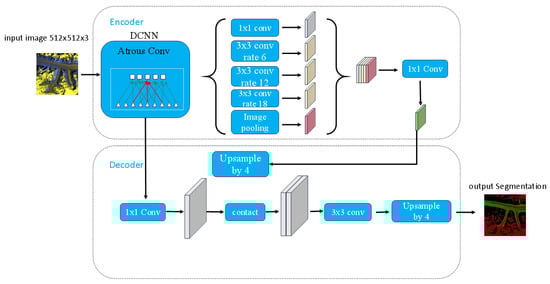
Figure 3.
The network structure of Deeplabv3+.
MobileNetV2 is a lightweight convolutional neural network designed for resource-constrained environments. It utilizes techniques such as inverted residuals, linear bottlenecks, and depthwise separable convolutions to reduce computational costs and parameter counts while maintaining strong feature representation capabilities [37]. For the small-scale dataset and relatively simple tasks in this study, MobileNetV2 efficiently meets accuracy requirements without causing unnecessary computational redundancy from over-parameterization.
In this research, MobileNetV2 was selected as the backbone for DeepLabV3+ to minimize overall computational demands. This choice is especially beneficial for real-time glacier segmentation in resource-limited settings, such as field deployments [38,39]. While MobileNetV2 may offer lower feature extraction capability compared to deeper models like ResNet or Xception, our experiments in the Tomur Peak region demonstrate its successful balance between segmentation accuracy and computational efficiency.
3.2.2. Accuracy Evaluation Method
To evaluate the accuracy of the glacier extraction methods mentioned above, this paper uses the revised RGI6.0 glacier boundary data as ground truth and selects precision, recall, mean Intersection over Union (MIoU), Mean Pixel Accuracy (MPA), and F1 Score as the accuracy evaluation metrics [40,41,42,43].
Based on the confusion matrix, the glacier extraction results are categorized into four types: TP (True Positive) refers to the number of glacier pixels (or pixels of other target categories) that the model correctly predicts as glacier pixels, i.e., the number of pixels predicted as positive (glacier) by the model and actually labeled as positive (glacier) in the ground truth; FP (False Positive) refers to the number of non-glacier pixels incorrectly predicted as glacier pixels by the model; TN (True Negative) refers to the number of pixels predicted as negative (non-glacier) by the model and actually labeled as negative (non-glacier); FN (False Negative) refers to the number of glacier pixels incorrectly predicted as non-glacier pixels by the model.
Precision is one of the key metrics for evaluating the classification performance of a model, and its expression is given by Equation (1). It represents the proportion of correctly predicted glacier samples out of all samples predicted as glaciers by the model.
Recall is a critical evaluation metric, and its expression is given by Equation (2). It measures the model’s effectiveness in identifying glacier pixels (typically the positive class). Specifically, recall refers to the proportion of correctly predicted positive samples out of all actual positive samples.
The mean Intersection over Union (MIoU) is an important evaluation metric in semantic segmentation, used to measure the model’s average segmentation performance across all categories. MIoU is calculated by averaging the Intersection over Union (IoU) for each category, and its expression is given by Equation (3), where N represents the total number of categories (in the case of the glacier multi-classification task, this includes debris-covered glaciers, glacial lakes, and pure glaciers).
The F1 Score is the harmonic mean of precision and recall, used to balance the trade-off between precision and recall in a classification model. Its expression is given by Equation (4).
4. Results
4.1. Glacier Boundary Extraction Classification Experiment
4.1.1. Comparison of Classification Results with Different Band Combinations
In existing studies, scholars have used different band combinations when constructing datasets. To determine the optimal band combination, this study conducts experiments with three band combinations on the 1989 imagery using the same deep learning model, constructing six datasets, each containing 860 images of 512 × 512 pixels. By keeping the model parameters and label files consistent, classification results with different band combinations are compared to identify the best band combination. The experimental results show that the dataset using the 345 band combination performs the best on the DeepLabv3+ model, with its MIoU improving by 0.37 to 3.52 percentage points compared to other band combinations. The specific results are shown in Table 2.
Table 2.
Comparison experiment of different band combinations.
Compared to the 541, 542, and 543 band combinations, the 145, 245, and 345 band combinations exhibit higher color contrast in image presentation. In this combination, the near-infrared band (Band 4) mapped to the green channel has higher brightness, while the short-wave infrared band (Band 5) mapped to the blue channel has lower brightness. This contrast enhances the visual distinction between glacial lakes and surrounding glaciers or rocks. Glaciers and snow reflect more in the red and near-infrared bands, while reflecting less in the short-wave infrared band, so glaciers appear yellow or light yellow in the image. In contrast, soil and exposed surfaces reflect more in the short-wave infrared band, and less in the red and near-infrared bands, resulting in a blue appearance. This band combination significantly improves the recognizability of glaciers.
Additionally, compared to methods using the blue (Band 1) and green (Band 2) band combinations, this paper selects the red (Band 3), near-infrared (NIR), and short-wave infrared (SWIR) band combination to construct the datasets. This combination performs exceptionally well in classifying glacier regions (as shown in Figure 4). It is noteworthy that the main classification errors for the three datasets are concentrated between debris-covered glaciers and pure glaciers, with error rates of 0.07, 0.09, and 0.1, respectively. This study indicates that, in glacier regions, the normalized index of the red band is typically lower, effectively distinguishing between ice and snow reflections and debris-covered glacier reflections. The classification results of this combination outperform the other two.
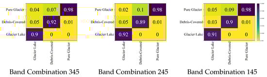
Figure 4.
Confusion matrix under different band combinations.
4.1.2. Comparison of Model Classification Results
To validate the effectiveness of the selected model, this study constructs a dataset based on 345-band data derived from satellite images acquired in 1989, 1992, and 2012. Five widely used semantic segmentation models are employed for comparative experiments: U-Net, DeepLabv3+, PSPNet, HRNet, and SegFormer (see Table 3). The experimental results indicate that DeepLabv3+, utilizing a MobileNet backbone, demonstrates significant accuracy advantages in glacier classification tasks. Its classification performance achieves a precision of 90.44%, recall of 82.75%, MIoU of 76.91%, and MPA of 82.75%. Compared to the other models, DeepLabv3+ shows an MIoU improvement ranging from 1.6 to 5.94 percentage points, underscoring its superior capability for glacier classification and extraction in medium-resolution optical remote sensing imagery.
Table 3.
Comparison experiment of different model.
Table 4 presents a comparison of the performance of different deep learning networks in three typical glacier feature extraction tasks. The comparative analysis clearly demonstrates that DeepLabv3+ excels in extracting complex features, such as glacier lakes, particularly when these lakes are small in size and fragmented in shape. This highlights DeepLabv3+’s distinct advantage in extracting fine-grained, irregularly shaped features, making it highly effective for small-scale, irregular target extraction tasks. Furthermore, DeepLabv3+ also performs strongly in extracting large-area features, such as pure glaciers, with key metrics such as precision and F1 Score significantly surpassing those of other models. This further underscores the model’s efficiency in handling large-scale, simple-structured features. Overall, DeepLabv3+ demonstrates a balanced and superior performance across various glacier feature extraction tasks, with particularly outstanding results in the segmentation of fine-grained and large-scale targets.
Table 4.
Comparison of classification results for different elements by various models.
Through a comparative analysis of the original imagery, label data, and classification results from five semantic segmentation models, which were then applied to the same dataset for the study area (as shown in Figure 5), it is evident that DeepLabv3+ significantly enhances detail extraction through multi-scale feature fusion. This is particularly demonstrated in the model’s performance in handling complex terrain and diverse glacier features, as shown in the following aspects.
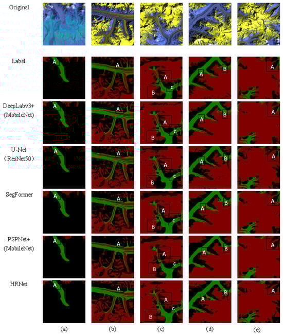
Figure 5.
The network structure of DeepLabv3+. (a–e) correspond to the first to fifth images, respectively. Letters A–C and the color marks indicate the regions of change.
Improved accuracy in shadowed mountain areas: For pure glaciers, especially in shadowed mountain regions, DeepLabv3+ significantly improves extraction accuracy. This advantage is evident in locations A and B in image block (Figure 5c), as well as in location A in Figure 5e. In these areas, the model effectively distinguishes glaciers from the surrounding environment, mitigating the common issue of misclassification in shadowed regions. The model leverages multi-scale feature fusion to fully exploit the spectral differences in shadowed areas, thereby improving classification accuracy.
Refined extraction of small debris glaciers: We find that, when extracting small debris-covered glaciers, DeepLabv3+ demonstrates greater precision and significantly reduces misclassification. This is evident in locations A in Figure 5b, location C in Figure 5c, and location A in Figure 5d. In these regions, glaciers share similar spectral characteristics with the surrounding environment (e.g., rocks and soil), making them challenging to extract using traditional methods. However, DeepLabv3+ improves the extraction performance of these complex areas by more effectively integrating both local and global contextual information, thus enhancing the overall extraction accuracy.
Enhanced continuity of narrow pure glaciers: For small, narrow pure glaciers embedded within debris-covered glaciers, DeepLabv3+ demonstrates improved coherence and consistency in the extraction process, significantly enhancing the accuracy of these slender glacier features. Notably, in location A in Figure 5a and location B in Figure 5d, DeepLabv3+ successfully reduces fragmentation and misclassification. Through multi-layered and multi-scale feature fusion, the model effectively strengthens its ability to recognize slender structures, further improving the accuracy of glacier extraction.
In summary, this study finds that DeepLabv3+ demonstrates outstanding performance in a variety of complex glacier extraction tasks through its multi-scale feature fusion advantages. It shows particularly powerful abilities in extracting small, slender, and shadowed regions, outperforming other models.
5. Discussion
5.1. Dynamic Change Monitoring and Analysis
Based on 18 remote sensing images acquired between 1989 and 2023, a statistical analysis of the classification results is conducted, and the resulting change trends are shown in Figure 6. In the Tomur Peak area, the overall trend for pure glaciers shows a decline, with fluctuations. However, in certain years, the glacier area shows a significant increase, primarily due to the interference of seasonal snow and classification errors caused by thick cloud cover. The trend for debris-covered glaciers, on the other hand, shows a slow upward trajectory, with an increase of 59.42 km2 over the 35-year period. This phenomenon is closely linked to the gradual rise in surface temperature and cumulative precipitation in the study area over the previous 34 years [19]. Furthermore, in some years, the decrease in the area of debris-covered glaciers may be attributed to seasonal snow covering the surface debris, which leads to the misidentification of these areas as pure glaciers by the classification model. In contrast, glacier lakes, due to their relatively small overall area, show no significant trend of change.
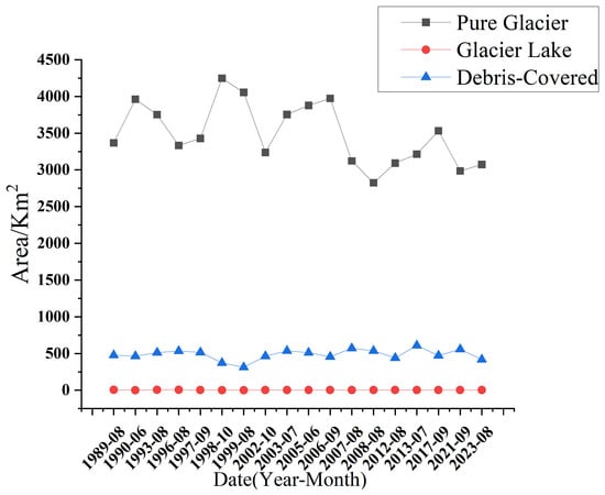
Figure 6.
Change trend in various feature areas from 1989 to 2023.
The process of glacier retreat is closely related to regional climate change. A climatic analysis conducted by Zhou et al. [19] for the Tomur Peak region from 1989 to 2023 indicates that, during the period 1989–2006, the region experienced a decreasing temperature trend and an increase in precipitation, which may have partially mitigated the rate of glacier mass loss. Further results from the Mann–Kendall trend test reveal that, since 2006, there has been a significant rise in temperature and a decline in precipitation, altering the accumulation-ablation balance and thereby accelerating glacier retreat. Notably, the trend in pure glacier area shown in Figure 6 closely aligns with these climatic shifts: between 1989 and 2006, the area remained relatively stable, whereas a marked decline has been observed since 2006, further confirming the critical role of climate factors in glacier dynamics.
In the study area, among the debris-covered glaciers, only the North Inylchek Glacier experienced a significant expansion in area between 1989 and 2023. This expansion was primarily due to a rapid advance of approximately 2404 m between 1996 and 1997 [44]. In contrast, glaciers such as the Tomur Glacier, Kaindy Glacier, Southern Inylchek Glacier, and Qiongkuziwayi Glacier, located on the southwest side of the Tomur Khantegri Mountain range, exhibit a marked reduction in area. This suggests that these glaciers have been significantly influenced by various environmental and climatic factors over the past 35 years. The areas of change are illustrated in Figure 7.
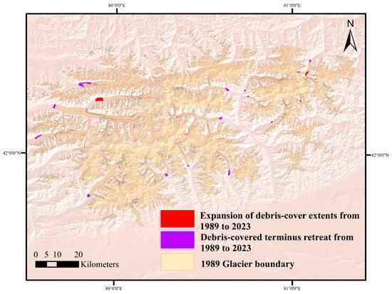
Figure 7.
Changes in debris-covered glacier areas in the Tomur Peak region from 1989 to 2023.
Glacier changes in the Tomur Peak region from 1989 to 2023 are presented in Table 5. In 1989, the total glacierized area was 3847.49 km2. Over the subsequent 35 years, this area shrank by 237.3 km2, corresponding to an average annual reduction rate of 6.97 km2·a−1 and a relative shrinkage rate of 0.18%·a−1.
Table 5.
Glacier change information in the Tomur Peak region from 1989 to 2023.
During the same period, the area of debris-covered glaciers expanded by 59.42 km2, representing a 12.4% increase relative to the 1989 area of 477.84 km2. In contrast, the glacier lake area shrank from 5.66 km2 to 2.22 km2, with an average annual retreat rate of 2.74%·a−1.
Climate factors are the primary drivers of glacier changes. Temperature predominantly influences glacier ablation, while precipitation plays a key role in the material supply to glaciers. Numerous studies have confirmed that temperature is the dominant factor influencing glacier dynamics. Additionally, it has been observed that, for every 1 °C increase in the summer average temperature, the amount of precipitation needed to compensate for glacier ablation increases by 40% to 50%. Data from the Wensu meteorological station indicate a significant rise in temperature since 1960, while the increase in precipitation has been comparatively slower [45]. This trend aligns with the ongoing glacier retreat observed in recent years.
5.2. Error Analysis and Model Sensitivity
To further assess the model’s adaptability and potential limitations in complex remote sensing environments, this section provides an in-depth analysis of the model’s classification performance in typical remote sensing scenarios, focusing on two key factors: cloud interference and sample imbalance. By comparing the reference labels with the model’s predictions, it can be observed that the model’s classification accuracy significantly decreases in areas covered by thick clouds, especially in the regions where pure glaciers are distributed, leading to higher rates of misclassification and omission. As shown in Figure 8, this phenomenon is mainly attributed to the severe obstruction of surface information by thick clouds, which significantly weakens the spectral contrast between glaciers and the surrounding background, making it difficult for the model to effectively extract discriminative features, thereby affecting the accuracy of the classification results.
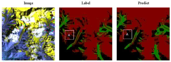
Figure 8.
Cloud-induced misclassification in glacier detection. A and the color marks indicate the regions of change.
The pixel count of the glacial lake category is significantly lower than that of other categories (see Table 6). This noticeable pixel imbalance has a considerable impact on the model’s classification accuracy, particularly for the glacial lake category, where the model tends to suffer from misclassification or omission. In the multi-class accuracy evaluation, the Deeplabv3+ model’s IoU for the glacial lake category is only 0.48, further indicating poor classification performance for this category. These results suggest that sample imbalance may be one of the key factors contributing to the model’s weaker performance on minority classes.
Table 6.
Pixel count for each category.
6. Conclusions
This study integrates medium-resolution satellite imagery with deep learning methods to achieve multi-class glacier classification and long-term change analysis in the Tomur Peak region from 1989 to 2023. The main conclusions are as follows.
Model Performance and Band Optimization: Comparative experiments show that the 345-band combination enhances image contrast, improving feature extraction for glacier areas. Among all the models, DeepLabv3+ (MobileNet) performs the best, with an MIoU improvement of 1.6 to 5.94 percentage points.
Glacier Change Patterns: From 1989 to 2023, glaciers in the Tomur Peak region exhibited a continuous retreat trend. During this period, the area of pure glaciers decreased by 296.72 km2, with a relative annual retreat rate of 0.26%·a−1. Meanwhile, the area of debris-covered glaciers increased by 59.42 km2, representing an approximate 12.4% expansion compared to 1989. The area of glacial lakes declined by 3.44 km2, corresponding to a relative annual retreat rate of 2.74%·a−1.
Compared with previous studies, this research also reveals a continuous retreat of glaciers in the Tomur Peak region. Zhou et al. [19] reported a 69.4 km2 increase in debris-covered glacier area from 1989 to 2022, which is slightly higher than the 59.42 km2 identified in this study. This discrepancy may be attributed to differences in study area boundaries or methodological approaches. He et al. [46] reported an average annual glacier retreat rate of 0.26%·a−1 for the Tomur Peak region during 1992–2017. Overall, these studies consistently indicate a sustained reduction in glacier area, reflecting the region’s increasing sensitivity to ongoing climate warming.
Limitations and Future Directions: Although the DeepLabv3+ model performs well, it faces under-segmentation issues for small targets such as glacier lakes and cloud-covered areas. Clouds obscure glaciers, reduce image quality, and cause spectral mixing, which affect boundary extraction and lead to misclassification. Future research will integrate multi-source data (e.g., high-resolution optical and radar imagery) and optimize model architecture to improve glacier extraction accuracy in complex environments.
Author Contributions
Methodology, Y.Z.; Software, Y.Z.; Validation, Y.Z.; Formal analysis, M.Z. and S.W.; Data curation, Y.H.; Writing—original draft, Y.Z.; Writing—review & editing, Y.Z. and F.H.; Supervision, F.H.; Funding acquisition, F.H. All authors have read and agreed to the published version of the manuscript.
Funding
This research received no external funding.
Institutional Review Board Statement
Not applicable.
Informed Consent Statement
Not applicable.
Data Availability Statement
The data presented in this study are available on request from the corresponding author.
Acknowledgments
The authors would like to thank the National Aeronautics and Space Administration (NASA), National Snow and Ice Data Center (NSIDC), United States Geological Survey (USGS), and European Space Agency (ESA) for providing free access to satellite imagery and reference data. The authors gratefully acknowledge the financial support provided by Qingzhan Zhao and the associated project, The project of the Xinjiang Production and Construction Corps Space Information Engineering Technology Center (2016BA001).
Conflicts of Interest
The authors declare no conflicts of interest.
References
- Bolch, T.; Kulkarni, A.; Kääb, A.; Huggel, C.; Paul, F.; Cogley, J.G.; Stoffel, M. The state and fate of Himalayan glaciers. Science 2012, 336, 310–314. [Google Scholar] [CrossRef] [PubMed]
- Cao, B.; Guan, W.; Li, K.; Wen, Z.; Han, H.; Pan, B. Area and Mass Changes of Glaciers in the West Kunlun Mountains Based on the Analysis of Multi-Temporal Remote Sensing Images and DEMs from 1970 to 2018. Remote Sens. 2020, 12, 2632. [Google Scholar] [CrossRef]
- Shean, D.E.; Bhushan, S.; Montesano, P.; Rounce, D.R.; Arendt, A.; Osmanoglu, B. A systematic, regional assessment of high mountain Asia glacier mass balance. Front. Earth Sci. 2020, 7, 363. [Google Scholar] [CrossRef]
- Yang, J.; Li, M.; Yang, S.; Tan, C. Vulnerability of the Glaciers to Climate Change in China:Current Situation and Evaluation. J. Glaciol. Geocryol. 2013, 35, 1077–1087. (In Chinese) [Google Scholar] [CrossRef]
- Xing, W.; Li, Z.; Zhang, H.; Zhang, M.; Liang, P.; Mou, J. Spatial-temporal variation of glacier resources in Chinese Tianshan Mountains since 1959. Acta Geogr. Sin. 2017, 72, 1594–1605. [Google Scholar] [CrossRef]
- Liu, S.; Yao, X.; Guo, W.; Xu, J.; Shangguan, D.; Wei, J.; Bao, W.; Wu, L. The Contemporary Glaciers in China Based on the Second Chinese Glacier Inventory. Acta Geogr. Sin. 2015, 70, 3–16. [Google Scholar] [CrossRef]
- Singh, S.; Tiwari, R.K.; Sood, V.; Kaur, R.; Prashar, S. The Legacy of Scatterometers: Review of Applications and Perspective. IEEE Geosci. Remote Sens. Mag. 2022, 10, 39–65. [Google Scholar] [CrossRef]
- Wang, S.; Zhang, M.; Li, Z.; Wang, F.; Li, H.; Li, Y.; Huang, X. Response of Glacier Area Variation to Climate Change in the Chinese Tianshan Mountains in the Past 50 Years. Acta Geogr. Sin. 2011, 66, 38–46. [Google Scholar] [CrossRef]
- Shen, Y.; Su, H.; Wang, G.; Mao, W.; Wang, S.; Han, P.; Wang, N.; Li, Z. The Responses of Glaciers and Snow Cover to Climate Change in Xinjiang (I): Hydrological Effects. J. Glaciol. Geocryol. 2013, 35, 513–527. [Google Scholar] [CrossRef]
- Shen, Y.; Su, H.; Wang, G.; Mao, W.; Wang, S.; Han, P.; Wang, N.; Li, Z. The Responses of Glaciers and Snow Cover to Climate Change in Xinjiang (II): Hazards Effects. J. Glaciol. Geocryol. 2013, 35, 1355–1370. [Google Scholar] [CrossRef]
- Zhang, M. Extracting the Temperate Glacier Information in Mount Namjagbarwa, Tibet Autonomous Region, Based on ETM+ Image. J. Glaciol. Geocryol. 2005, 27, 226–232. (In Chinese) [Google Scholar] [CrossRef]
- Gao, J.; Yao, T.; Masson-Delmotte, V.; Steen-Larsen, H.C.; Wang, W. Collapsing Glaciers Threaten Asia’s Water Supplies. Nature 2019, 565, 19–21. [Google Scholar] [CrossRef] [PubMed]
- Jacob, T.; Wahr, J.; Pfeffer, W.T.; Swenson, S. Recent Contributions of Glaciers and Ice Caps to Sea Level Rise. Nature 2012, 482, 514–518. [Google Scholar] [CrossRef]
- Gao, K.; Kääb, A.; Leinss, S.; Gilbert, A.; Bühler, Y.; Gascoin, S.; Evans, S.G.; Yao, T. Massive Collapse of Two Glaciers in Western Tibet in 2016 After Surge-Like Instability. Nat. Geosci. 2018, 11, 114–120. [Google Scholar] [CrossRef]
- Zhou, Y.; Li, X.; Zheng, D.; Li, Z.; An, B.; Wang, Y.; Jiang, D.; Su, J.; Cao, B. The Joint Driving Effects of Climate and Weather Changes Caused the Chamoli Glacier-Rock Avalanche in the High Altitudes of the India Himalaya. Sci. China Earth Sci. 2021, 64, 1909–1921. [Google Scholar] [CrossRef]
- Veh, G.; Korup, O.; von Specht, S.; Roessner, S.; Walz, A. Unchanged Frequency of Moraine-Dammed Glacial Lake Outburst Floods in the Himalaya. Nat. Clim. Change 2019, 9, 379–383. [Google Scholar] [CrossRef]
- Zhang, C.; Yue, P.; Tapete, D.; Shangguan, B.; Wang, M.; Wu, Z. A Multi-Level Context-Guided Classification Method with Object-Based Convolutional Neural Network for Land Cover Classification Using Very High Resolution Remote Sensing Images. Int. J. Appl. Earth Obs. Geoinf. 2020, 88, 102086. [Google Scholar] [CrossRef]
- Gu, H.; Han, Y.; Yang, Y.; Li, H.; Liu, Z.; Soergel, U.; Blaschke, T.; Cui, S. An Efficient Parallel Multi-Scale Segmentation Method for Remote Sensing Imagery. Remote Sens. 2018, 10, 590. [Google Scholar] [CrossRef]
- Zhou, W.; Xu, M.; Han, H. Spatial Distribution and Variation in Debris Cover and Flow Velocities of Glaciers during 1989–2022 in Tomur Peak Region, Tianshan Mountains. Remote Sens. 2024, 16, 2587. [Google Scholar] [CrossRef]
- Paul, F. Evaluation of different methods for glacier mapping using Landsat TM. EARSeL eProc. 2000, 1, 239–245. [Google Scholar]
- Bhambri, R.; Bolch, T.; Chaujar, R.K.; Kulshreshtha, S.C. Glacier changes in the Garhwal Himalaya, India, from 1968 to 2006 based on remote sensing. J. Glaciol. 2011, 57, 543–556. [Google Scholar] [CrossRef]
- Paul, F.; Kääb, A.; Haeberli, W. Recent glacier changes in the Alps observed by satellite: Consequences for future monitoring strategies. Glob. Planet. Change 2007, 56, 111–122. [Google Scholar] [CrossRef]
- Chand, P.; Sharma, M.C. Glacier changes in the Ravi basin, North-Western Himalaya (India) during the last four decades (1971–2010/13). Glob. Planet. Change 2015, 135, 133–147. [Google Scholar] [CrossRef]
- Shelhamer, E.; Long, J.; Darrell, T. Fully Convolutional Networks for Semantic Segmentation. IEEE Trans. Pattern Anal. Mach. Intell. 2017, 39, 640–651. [Google Scholar] [CrossRef]
- Mohajerani, Y.; Wood, M.; Velicogna, I.; Rignot, E. Detection of Glacier Calving Margins with Convolutional Neural Networks: A Case Study. Remote Sens. 2019, 11, 74. [Google Scholar] [CrossRef]
- Davari, A.; Baller, C.; Seehaus, T.; Braun, M.; Maier, A.; Christlein, V. Pixelwise Distance Regression for Glacier Calving Front Detection and Segmentation. IEEE Trans. Geosci. Remote Sens. 2022, 60, 5224610. [Google Scholar] [CrossRef]
- Xie, Z.; Haritashya, U.K.; Asari, V.K.; Young, B.W.; Bishop, M.P.; Kargel, J.S. GlacierNet: A Deep-Learning Approach for Debris-Covered Glacier Mapping. IEEE Access 2020, 8, 83495–83510. [Google Scholar] [CrossRef]
- Wang, Z.; Wang, Z.; You, S.; Lei, F.; Cao, L.; Yang, K. Landsat Image Glacier Extraction Based on Context Semantic Segmentation Network. Acta Geod. Cartogr. Sin. 2020, 49, 1575–1582. (In Chinese) [Google Scholar] [CrossRef]
- Zhang, D.; Fan, H.; Kang, B.; Gao, J.; Li, T. Glacier Remote Sensing Image Detection Method under Complex Background Based on Improved U-Net Network. J. Appl. Basic Eng. Sci. 2022, 4, 806–818. (In Chinese) [Google Scholar] [CrossRef]
- Zhou, Y.; Wang, Y.; Zhou, W. Monitoring Glacier Area Change in Tianshan Mountains Based on Remote Sensing Images. Min. Surv. 2012, 3, 21–25. (In Chinese) [Google Scholar] [CrossRef]
- Lei, S.; Fang, L.; Li, C.; Yang, M. Improved Algorithm for Extracting Debris-Covered Glacier Regions in Optical Satellite Images. Comput. Eng. 2025, 51, 269–277. [Google Scholar] [CrossRef]
- Chen, Y.; Ji, X. Comparative Study of Glacier Identification Methods Based on Landsat 8 OLI Images. Front. Earth Sci. 2017, 7, 812–818. (In Chinese) [Google Scholar] [CrossRef]
- Herreid, S.; Pellicciotti, F. The State of Rock Debris Covering Earth’s Glaciers. Nat. Geosci. 2020, 13, 621–627. [Google Scholar] [CrossRef]
- Chen, G.; Zhang, X.; Wang, Q.; Dai, F.; Gong, Y.; Zhu, K. Symmetrical Dense-Shortcut Deep Fully Convolutional Networks for Semantic Segmentation of Very-High-Resolution Remote Sensing Images. IEEE J. Sel. Top. Appl. Earth Obs. Remote Sens. 2018, 11, 1633–1644. [Google Scholar] [CrossRef]
- Pereira, T.D.; Tabris, N.; Matsliah, A.; Turner, D.M.; Li, J.; Ravindranath, S.; Papadoyannis, E.S.; Normand, E.; Deutsch, D.S.; Wang, Z.Y.; et al. SLEAP: A Deep Learning System for Multi-Animal Pose Tracking. Nat. Methods 2022, 19, 486–495. [Google Scholar] [CrossRef]
- Emek Soylu, B.; Guzel, M.S.; Bostanci, G.E.; Ekinci, F.; Asuroglu, T.; Acici, K. Deep-Learning-Based Approaches for Semantic Segmentation of Natural Scene Images: A Review. Electronics 2023, 12, 2730. [Google Scholar] [CrossRef]
- Rybczak, M.; Kozakiewicz, K. Deep Machine Learning of MobileNet, Efficient, and Inception Models. Algorithms. 2024, 17, 96. [Google Scholar] [CrossRef]
- Mo, L.; Fan, Y.; Wang, G.; Yi, X.; Wu, X.; Wu, P. DeepMDSCBA: An Improved Semantic Segmentation Model Based on DeepLabV3+ for Apple Images. Foods. 2022, 11, 3999. [Google Scholar] [CrossRef]
- Wang, Y.; Yang, L.; Liu, X.; Yan, P. An Improved Semantic Segmentation Algorithm for High-Resolution Remote Sensing Images Based on DeepLabv3+. Sci. Rep. 2024, 14, 9716. [Google Scholar] [CrossRef]
- Deng, X.; Liu, Q.; Deng, Y.; Mahadevan, S. An Improved Method to Construct Basic Probability Assignment Based on the Confusion Matrix for Classification Problem. Inf. Sci. 2016, 340, 250–261. [Google Scholar] [CrossRef]
- Chicco, D.; Jurman, G. The Advantages of the Matthews Correlation Coefficient (MCC) over F1 Score and Accuracy in Binary Classification Evaluation. BMC Genom. 2020, 21, 6. [Google Scholar] [CrossRef] [PubMed]
- Rezatofighi, H.; Tsoi, N.; Gwak, J.; Sadeghian, A.; Reid, I.; Savarese, S. Generalized Intersection over Union: A Metric and a Loss for Bounding Box Regression. In Proceedings of the IEEE/CVF Conference on Computer Vision and Pattern Recognition, Long Beach, CA, USA, 15–20 June 2019; pp. 658–666. [Google Scholar]
- Chen, L.C.; Papandreou, G.; Kokkinos, I.; Murphy, K.; Yuille, A.L. DeepLab: Semantic Image Segmentation with Deep Convolutional Nets, Atrous Convolution, and Fully Connected CRFs. IEEE Trans. Pattern Anal. Mach. Intell. 2018, 40, 834–848. [Google Scholar] [CrossRef] [PubMed]
- Zhou, S.; Yao, X.; Zhang, D.; Zhang, Y.; Liu, S.; Min, Y. Remote Sensing Monitoring of Advancing and Surging Glaciers in the Tien Shan, 1990–2019. Remote Sens. 2021, 13, 1973. [Google Scholar] [CrossRef]
- Yang, S.; Wang, F.; Xie, Y.; Zhao, W.; Bai, C.; Liu, J.; Xu, C. Delineation Evaluation and Variation of Debris-Covered Glaciers Based on the Multi-Source Remote Sensing Images, Take Glaciers in the Eastern Tomur Peak Region for Example. Remote Sens. 2023, 15, 2575. [Google Scholar] [CrossRef]
- He, X.; Liu, B.; Feng, Z. Glacier Variations in Response to Climate Change in the Karlik Mountain from 1990 to 2020. Remote Sens. Technol. Appl. 2024, 39, 1373–1382. (In Chinese) [Google Scholar] [CrossRef]
Disclaimer/Publisher’s Note: The statements, opinions and data contained in all publications are solely those of the individual author(s) and contributor(s) and not of MDPI and/or the editor(s). MDPI and/or the editor(s) disclaim responsibility for any injury to people or property resulting from any ideas, methods, instructions or products referred to in the content. |
© 2025 by the authors. Licensee MDPI, Basel, Switzerland. This article is an open access article distributed under the terms and conditions of the Creative Commons Attribution (CC BY) license (https://creativecommons.org/licenses/by/4.0/).