Decomposition and Decoupling Analysis of the Driving Factors of the “Water–Carbon–Ecological” Footprint in the Eleven Provinces and Municipalities of the Yangtze River Economic Belt

Abstract

Studying the spatio-temporal evolution characteristics of the “water–carbon–ecological” footprint and the decoupling status of its main driving factors is of paramount importance for achieving sustainable development in society. Based on quantifying the footprint family, this study constructs an integrated driving factor analysis model of “Kaya–LMDI–Tapio”, screens the main driving factors influencing the footprint family, and conducts decoupling analysis. The research results indicate that: (1) The water, carbon, and ecological footprints of the Yangtze River Economic Belt from 2002 to 2017 were 1534.265 billion cubic meters, 61,672.89 million hectares, and 45,528.76 million hectares, respectively. (2) The main driving factors for water, carbon, and ecological footprints were economic effect factors, agricultural production scale factors, and economic effect factors. (3) During the research period, the decoupling trends between the water, carbon, and ecological footprints and their main driving factors presented a transformation from a weak decoupling state to a strong decoupling state, the decoupling index value decreased initially and then increased, and the decoupling index value showed a downward trend. These findings provide a quantitative basis for the formulation of differentiated basin management policies, indicating that, through the collaborative promotion of technological innovation and institutional innovation, the leap from relative decoupling to absolute decoupling can be achieved, which has important reference value for the sustainable development governance of global river basins.

1. Introduction

The scientific measurement of the impact of human activities on resources and the environment is of crucial importance in addressing global issues such as climate change, resource shortage, and environmental pollution. The study of the footprint family can quantify the environmental pressure generated by human activities, reveal the bottlenecks and challenges of sustainable development, and thereby provide a scientific basis for achieving sustainable development in society [1,2]. The concept of the footprint originated from the ecological footprint proposed by Wackernagel and Rees in 1992. Over the past two decades, concepts such as water footprint, carbon footprint, and energy footprint have been put forward based on the ecological footprint, making the footprint concept more comprehensive and eventually forming the concept of the footprint family [3,4].

At present, the calculation of the water footprint mainly proceeds from the perspective of the production of crops and other products, employing both bottom-up and top-down methods in combination with input–output tables to calculate the regional water footprint value [1,5,6]. Ma et al. (2024) evaluated the spatio-temporal patterns of agricultural blue water and green water footprints of six crops in the lower reaches of the Yangtze River Economic Belt (YREB) based on the Penman–Monteith model–Monteith method and constructed composite scarcity indices of agricultural water, agricultural blue water, and agricultural green water footprints to assess the agricultural water security level of blue and green water resources in the lower reaches of the YREB [7].

The calculation of the carbon footprint mainly adopts the IPCC coefficient method to calculate the carbon footprint value resulting from energy consumption. Tian et al. (2024), using remote sensing datasets of fossil fuel carbon emissions and vegetation carbon sequestration, revealed China’s carbon footprint pressure from 2005 to 2021 [8].

The traditional two-dimensional ecological footprint struggles to accurately measure the current flow of natural capital. Niccolucci et al. (2011) introduced the concepts of footprint depth and footprint breadth and proposed a three-dimensional ecological footprint model to identify the occupation of regional natural capital stock and the consumption of natural capital flow [9]. Wang et al. (2024) conducted a multi-scale analysis of sustainability in the YREB based on the three-dimensional ecological footprint (EF) model [10].

LMDI and Tapio, as common driving factor decomposition models, are frequently used in the analysis of carbon emission driving factors. Lin and Li (2024) adopted the Kaya–LMDI–SD–MC framework to conduct a systematic analysis and dynamic prediction of the carbon emission peak of residential buildings in Fujian Province and explore emission reduction paths [11]. Liu et al. (2024) employed the Tapio model to construct a decoupling index based on factor decomposition and analyzed the driving factors and decoupling status of changes in China’s construction industry from 2000 to 2020 [12].

In summary, although the current research on regional water footprints, carbon footprints, etc. has laid a solid foundation for this study, there are still obvious gaps: (1) The current research on the spatio-temporal evolution of water footprints and carbon footprints often focuses on the footprint values of single industries such as agriculture, industry, and energy consumption, ignoring the changes in the footprint family caused by life and ecology. (2) The current research on regional footprint driving factors mainly concentrates on single footprints such as carbon footprint and ecological footprint, with the focus on reducing carbon emissions in industries. However, the study of the footprint family and its significance in achieving regional sustainable development is often overlooked. (3) The research on driving factors often focuses on a single study of driving factor decomposition or decoupling, neglecting the decoupling analysis of the main driving factors. It is necessary to conduct decoupling analysis on the driving factors with the highest contribution degree.

Taking 11 provinces and cities along the YREB as the research object, this study innovatively constructs a multi-dimensional coupled analysis framework of “W-C-E”, breaking through the limitations of existing studies that focus on single factors or pairiness. By integrating the LMDI decomposition method and Tapio decoupling model, the dynamic decomposition and spatio-temporal evolution analysis of regional resources and environmental pressure are realized, which has obvious advantages compared with traditional static research methods. In terms of spatial scale, this study focuses on the integrity of the watershed economic belt and the differences among sections and especially examines the influence of regional policy factors such as industrial transfer and ecological compensation, which makes up for the shortcomings of the national scale or single province research. Compared with previous studies, this study has significant innovations in three aspects:

First, it realizes the coupling analysis of a ternary system of water resources, carbon emission, and ecological footprint for the first time at the basin scale.

The second is the use of the latest aging data (until 2022) to reflect the characteristics of the new development stage. The third is the building of a differentiated evaluation index system suitable for the Yangtze River Economic Belt. At the same time, this study inherits and develops the IPAT-STIRPAT model framework, complements the Yangtze River Delta, Chengdu–Chongqing, and other subregional studies, and provides regional empirical support for national strategies such as Yangtze River conservation and dual-carbon targets. By systematically revealing the heterogeneity of driving factors in the upper, middle, and lower reaches and the evolution law of the decoupling state, it not only enriches the theoretical methods of resource and environmental economics but also provides a scientific basis and policy inspiration for promoting the green coordinated development of the YREB.

This study aims to fill the current research gaps by introducing the Kaya–LMDI–Tapio framework, comprehensively calculating the spatio-temporal evolution characteristics of the footprint family, and conducting driving factor analysis of the footprint family. Firstly, based on the industrial structure of the YREB, the spatio-temporal evolution characteristics of the footprint family for the eleven provinces and municipalities were comprehensively calculated. Then, the contribution degree of each driving factor in the footprint family was calculated using the Kaya–LMDI method, quantitatively analyzing the key driving factors of the footprint family and conducting decoupling analysis on the key driving factors separately. Finally, based on the contribution degree of the driving factors and the decoupling results, policy recommendations were proposed for the sustainable development of the YREB.

The structure of this study is as follows. Section 2 outlines the calculation structure, research methods, and data sources of the footprint family. Section 3 presents the calculation results. Section 3 presents the analysis and discussion. Finally, Section 4 is the conclusion.

2. Materials and Methods

In this study, an innovative Kaya–LMDI–Tapio integrated analysis framework was constructed to systematically investigate the driving mechanism and decoupling characteristics of the “water–carbon–ecological” footprint in the Yangtze River Economic Belt. This approach has three significant advantages:

Firstly, at the level of theoretical construction, Kaya identity deconstructs the complex environmental pressure into the product relationship of core factors such as population, economy, and technology through mathematical modeling, providing a rigorous theoretical framework for the analysis of multi-dimensional environmental effects. We further extend the scope of application of the traditional Kaya identity, and for the first time apply it to the ternary system analysis of water resources, carbon emissions, and ecological footprint simultaneously.

Secondly, at the level of method innovation, the LMDI decomposition method is used to achieve accurate quantification of driving factors. In particular, the additive decomposition form (LMDI-I) was chosen in this study, whose complete decomposition characteristics ensured the unbiased results, while the multiplicative decomposition (LMDI-II) was used for sensitivity testing. This combination of methods significantly improved the reliability of the research conclusions.

Third, at the policy application level, the spatial dynamic analysis function of the Tapio decoupling model enables us to identify the differentiated decoupling status of the three sections of the Yangtze River Economic Belt, upper, middle, and lower reaches. For example, the Yangtze River Delta region has shown strong decoupling characteristics, while the provinces in the middle reaches are still in the weak decoupling stage, which provides an important basis for formulating regional differentiated environmental policies.

2.1. Computational Approach for Water Footprint

In this research, the water footprint was classified and calculated as blue water footprint and green water footprint. The blue water footprint encompasses those of the industrial, agricultural, domestic, and ecological sectors. Herein, for the industrial sector, given the wide variety of industrial products, industrial water consumption was adopted as a surrogate. The domestic and ecological sectors mainly consume blue water, and thus the water consumption data for both were utilized to represent their blue water footprints. The blue water footprint for the agricultural sector was mainly determined based on the evapotranspiration during the crop growth period. The principal crops included: Legumes, oilseeds, wheat, corn, rice, and vegetables [7]. The green water footprint refers to the precipitation consumed during the crop production process. In this paper, the regional green water footprint was calculated using the evapotranspiration during the crop growth period. The calculation formula is as follows:

$${WF}_{blue}=10{ET}_{blue}/Y$$

(1)

$$E{T}_{blue}=\max \left(0,E{T}_c-P_{eff}\right)$$

(2)

$$E{T}_c=K_c\times E{T}_0$$

(3)

$${ET}_0={\displaystyle \frac{0.408\Delta \left(R_n-G\right)+\gamma \frac{900}{T+273}{U}_2\left(e_s-e_a\right)}{\Delta +\gamma \left(1+0.34U_2\right)}}$$

(4)

$$P_{eff,dec}=\left\{\begin{array}{ll}{P}_{\mathrm{dec}}\times \left(125-0.6\times P_{\mathrm{dec}}\right)/125\hfill & P_{\mathrm{dec}}\le (250/3)\mathrm{mm}\hfill \\ 125/3+0.1\times P_{\mathrm{dec}}\hfill & P_{\mathrm{dec}}>(250/3)\mathrm{mm}\hfill \end{array}\right.$$

(5)

$${WF}_{green}=10{ET}_{green}/Y$$

(6)

$$WF={WF}_{green}+{WF}_{blue}$$

where ${WF}_{blue}$ is the blue water footprint, ${ET}_{blue}$ is the blue water evapotranspiration, $Y$ is the yield per unit area of a certain crop (t/hm²), 10 is the conversion coefficient, $P_{eff}$ is the effective rainfall, $P_{dec}$ is the ten-day rainfall, and $K_c$ is the crop coefficient.

2.2. Computational Method for Carbon Footprint

2.2.1. Carbon Emissions

In this study, carbon emissions are calculated through the assessment of energy consumption and agricultural production. Specifically, the carbon footprint of energy encompasses those resulting from the consumption of raw coal, coke, crude oil, gasoline, kerosene, diesel, fuel oil, liquefied petroleum gas, and natural gas. The carbon footprint of agriculture comprises those generated by the usage of agricultural fertilizers, pesticides, agricultural films, the sown area of crops, the total power of agricultural machinery, the effective irrigated area of farmland, and the diesel consumption of agricultural machinery [9,13]. The calculation formula is as follows:

$$C={\displaystyle \sum _i^n{G}_i\times {\beta }_i\times {\delta }_i}$$

(7)

where C stands for the total amount of carbon dioxide emissions resulting from energy consumption, $G_i$ denotes the consumption of the ith type of energy, ${\beta }_i$ represents the conversion coefficient of the ith type of energy to standard coal, and ${\delta }_i$ indicates the carbon emission coefficient of the ith type of energy.

$$E=G_{\mathrm{f}}A+G_{\mathrm{p}}B+G_{\mathrm{m}}C+\left(A_{\mathrm{e}}D+W_{\mathrm{e}}F\right)+A_{\mathrm{ir}}G+G_{\mathrm{s}}J$$

(8)

where $E$ denotes the total carbon emissions from farmland within the region, $G_{\mathrm{f}}$ indicates the usage of agricultural fertilizers, $G_{\mathrm{p}}$ indicates the usage of pesticides, $G_{\mathrm{m}}$ indicates the usage of agricultural plastic film, $A_{\mathrm{e}}$ indicates the sown area of crops, $W_{\mathrm{e}}$ indicates the total power of agricultural machinery, $A_{\mathrm{ir}}$ indicates the effective irrigation area of farmland, $G_{\mathrm{s}}$ indicates the usage of diesel for agricultural machinery, and A, B, C, D, F, G, J represent the carbon emission coefficient.

2.2.2. Carbon Absorption

In this study, the carbon absorption is computed by calculating the carbon absorption of crops and land. Among them, the agricultural carbon absorption encompasses the calculation of the carbon absorption capacity of the crop ecosystem throughout its entire life cycle by utilizing the crop yield, corresponding economic coefficient, moisture content, carbon content, and root–shoot ratio. The carbon absorption of land includes the carbon absorption capabilities of forest land, grassland, water areas, and wetlands [8]. The calculation formula is as follows:

$$W_1={\displaystyle \sum _{i=1}^n{W}_{1i}}={\displaystyle \sum _{i=1}^n\left[C_i\times Y_i\times \left(1-V_i\right)\times \left(1+R_i\right)\right]}/H_i$$

(9)

where $W_1$ represents the total carbon absorption of the regional farmland ecosystem, $C_i$ represents the carbon content rate of the ith type of crop, $Y_i$ represents the fresh matter mass of the ith type of crop harvested, $V_i$ represents the moisture content of the ith type of crop, $R_i$ represents the root–shoot ratio coefficient of the ith type of crop, and $H_i$ represents the economic coefficient of the ith type of crop.

$$W_2={\displaystyle \sum _{i=1}^n{W}_{2i}}={\displaystyle \sum _{i=1}^n{U}_i\times V_i}$$

(10)

where $W_2$ denotes the total carbon absorption of the regional land, $U_i$ indicates the area of the ith type of land use, and $V_i$ indicates the carbon absorption coefficient of the ith type of land use.

$$CF=E+W_1+W_2$$

2.3. Computational Method for Ecological Footprint

In this study, a three-dimensional ecological footprint model is employed, introducing footprint depth and footprint breadth to distinguish between the depletion of natural capital stocks and the appropriation of capital flows, remedying the shortcomings of the traditional two-dimensional ecological footprint model. The land use types are categorized into six major types: Cultivated land, forest land, grassland, water areas, fossil energy land, and construction land for calculating the ecological footprint values [10,14]. The types of ecological footprint products and the division of productive land in the eleven provinces and cities in the YREB are presented in

Table 1. Product Types of Ecological Footprint and Division of Productive Land in the eleven provinces and cities in the YREB.

Account of Biological Resources	Product	Energy Account	Product
Cultivated land	Soybeans, oilseeds, wheat, corn, rice, vegetables, potatoes, cotton, flax, tobacco, sugar beets	Land for fossil energy	Raw coal, coke, crude oil, gasoline, kerosene, diesel, fuel oil, liquefied petroleum gas, and natural gas
Forest land	Tea, fruits
Grassland	Pork, beef, lamb, milk, and eggs	Construction land	Electricity
Water area	Aquatic products

.

$$E{F}_{\mathrm{depth}}=1+{\displaystyle \frac{ED}{BC}}=1+{\displaystyle \frac{{\displaystyle \sum _{i=1}^{\mathrm{n}}\max }\left\{E{F}_i-B{C}_i,0\right\}}{{\displaystyle \sum _{i=1}^{\mathrm{n}}B}{C}_i}}$$

(11)

$$E{F}_{\mathrm{size}}={\displaystyle \sum _{i=1}^{\mathrm{n}}\min }\left\{E{F}_i,B{C}_i\right\}$$

(12)

$$E{F}_{3\mathrm{D}}=E{F}_{\mathrm{depth}}\times E{F}_{\mathrm{size}}$$

(13)

where $E{F}_{\mathrm{depth}}$ denotes the depth of the footprint, $E{F}_{\mathrm{size}}$ denotes the breadth of the footprint, $B{C}_i$ denotes the ecological carrying capacity of different land types, and $E{F}_{3\mathrm{D}}$ denotes the three-dimensional ecological footprint.

2.4. “Water–Carbon–Ecosystem” Footprint Kaya–LMDI Driving Factor Decomposition

This study establishes a driving factor model based on the theoretical framework of the system, which is mainly based on three theoretical systems: First, the nonlinear relationship between economic growth and environmental pressure is explained from the perspective of development stage; secondly, construct the multi-dimensional technological progress influence mechanism; thirdly, according to the theory of new economic geography, the conduction path of space spillover effect to environmental pressure is revealed. In the model selection, three theoretical requirements are mainly considered: Dynamic modeling is required for path-dependent characteristics of environmental systems, a structural equation framework is required for interaction effects between elements, and variable coefficient analysis is required for regional heterogeneity. These theoretical innovations enable the model to capture the direct effects, indirect effects, and spatial spillovers of drivers more completely and provide a new analytical perspective for understanding complex environmental economic systems.

The Kaya method was established by Yoichi Kaya in 1989 and is primarily utilized as a fundamental framework for analyzing the determinants of CO₂ emissions. It offers flexibility for expansion or adjustment in accordance with specific research objectives, permitting the inclusion of additional variables tailored to the research focus. The LMDI approach is preferred in energy and environmental studies due to its solid theoretical basis, ease of result interpretation, and flexibility [15,16]. In this research, the Kaya–LMDI method from the footprint family was employed for driving factor analysis.

2.4.1. Water Footprint Kaya–LMDI Factor Decomposition Method

In this study, the LMDI decomposition model for the water footprint of the eleven provinces and cities in the YREB was constructed using the factors of technological progress, economic effects, and population size as follows:

$${WF}_t={\displaystyle \sum _{i=1}^4\frac{{WF}_t}{E_t}\frac{E_t}{P_t}{P}_t}={\displaystyle \sum S_t^{WF}{Q}_t^{WF}{P}_t^{WF}}$$

(14)

$$\begin{array}{l}\Delta WF=W{F}_t-W{F}_0={\displaystyle \sum S_{\mathrm{it}}^{WF}{Q}_t^{WF}{P}_t^{WF}}-{\displaystyle \sum S_{i0}^{WF}{Q}_0^{WF}{P}_0^{WF}}\\ =\Delta W{F}_S+\Delta W{F}_I+\Delta W{F}_Q+\Delta W{F}_P\end{array}$$

(15)

$$\Delta W{F}_S={\displaystyle \sum \frac{W{F}_t-W{F}_0}{\ln W{F}_t-\ln W{F}_0}}\cdot ln{\displaystyle \frac{S_t}{S_0}}$$

(16)

$$\Delta W{F}_Q={\displaystyle \sum \frac{W{F}_t-W{F}_0}{\ln W{F}_t-\ln W{F}_0}}\cdot ln{\displaystyle \frac{Q_t}{Q_0}}$$

(17)

$$\Delta W{F}_P={\displaystyle \sum \frac{W{F}_t-W{F}_0}{\ln W{F}_t-\ln W{F}_0}}\cdot ln{\displaystyle \frac{P_t}{P_0}}$$

(18)

where $E_t$ and $P_t$ respectively represent the gross domestic product (GDP) and population size of different cities, $S_t$ represents the relationship between water footprint and GDP, $Q_t$ represents per capita GDP, $\Delta W{F}_S$, $\Delta W{F}_Q$, and $\Delta W{F}_P$ respectively represent the contribution of technological progress factors, economic effect factors, and population size factors to the water footprint.

2.4.2. Carbon Footprint Kaya–LMDI Factor Decomposition Method

In this study, the LMDI decomposition model for the carbon footprint of the eleven provinces and cities in the YREB, which was constructed using factors such as the intensity of energy carbon emissions, technological progress, the scale of agricultural production, agricultural production efficiency, land area, and population size, is as follows:

$${CF}_t={\displaystyle \sum \frac{{CF}_t}{N_t}\frac{N_t}{E_t}\frac{E_t}{F_t}}{\displaystyle \frac{F_t}{W_t}}{\displaystyle \frac{W_t}{P_t}}{P}_t={\displaystyle \sum C_t^{CF}{H}_t^{CF}{K}_t^{CF}{X}_t^{CF}{Y}_t^{CF}{P}_t^{CF}}$$

(19)

$$\Delta CF=C{F}_t-C{F}_0={\displaystyle \sum C_t^{CF}{H}_t^{CF}{K}_t^{CF}{X}_t^{CF}{Y}_t^{CF}{P}_t^{CF}}-{\displaystyle \sum C_0^{CF}{H}_0^{CF}{K}_0^{CF}{X}_0^{CF}{Y}_0^{CF}{P}_0^{CF}}$$

(20)

$$=\Delta C{F}_C+\Delta C{F}_H+\Delta C{F}_K+\Delta C{F}_X+\Delta C{F}_Y+\Delta C{F}_P$$

(21)

$$\Delta C{F}_C={\displaystyle \sum \frac{C{F}_t-C{F}_0}{\ln C{F}_t-\ln C{F}_0}}\cdot ln{\displaystyle \frac{{C^{CF}}_t}{C_0^{CF}}}$$

(22)

$$\Delta C{F}_H={\displaystyle \sum \frac{C{F}_t-C{F}_0}{\ln C{F}_t-\ln C{F}_0}}\cdot ln{\displaystyle \frac{{H^{CF}}_t}{H_0^{CF}}}$$

(23)

$$\Delta C{F}_K={\displaystyle \sum \frac{C{F}_t-C{F}_0}{\ln C{F}_t-\ln C{F}_0}}\cdot ln{\displaystyle \frac{{K^{CF}}_t}{K_0^{CF}}}$$

(24)

$$\Delta C{F}_X={\displaystyle \sum \frac{C{F}_t-C{F}_0}{\ln C{F}_t-\ln C{F}_0}}\cdot ln{\displaystyle \frac{{X^{CF}}_t}{X_0^{CF}}}$$

(25)

$$\Delta C{F}_Y={\displaystyle \sum \frac{C{F}_t-C{F}_0}{\ln C{F}_t-\ln C{F}_0}}\cdot ln{\displaystyle \frac{{Y^{CF}}_t}{Y_0^{CF}}}$$

(26)

$$\Delta C{F}_P={\displaystyle \sum \frac{C{F}_t-C{F}_0}{\ln C{F}_t-\ln C{F}_0}}\cdot ln{\displaystyle \frac{{P^{CF}}_t}{P_0^{CF}}}$$

(27)

where, $N_t$, $F_t$, and $W_t$ respectively represent the energy consumption, grain production, and productive land area of different cities. $C_t$ represents the relationship between carbon footprint and energy consumption. $H_t$ represents the relationship between energy consumption and GDP. $K_t$ represents the relationship between GDP and grain production. $X_t$ represents the relationship between grain production and productive land area. $Y_t$ represents the per capita land area. $\Delta C{F}_C$, $\Delta C{F}_H$, $\Delta C{F}_K$, $\Delta C{F}_X$, $\Delta C{F}_Y$, and $\Delta C{F}_P$ respectively denote the factors of energy carbon emission intensity, energy consumption intensity, agricultural production scale, agricultural production efficiency, land area, and population scale.

2.4.3. Ecological Footprint Kaya–LMDI Factor Decomposition Method

The LMDI decomposition model for the ecological footprint of the eleven provinces and cities in the YREB, constructed using structural factors, technological progress factors, economic effect factors, and population scale factors, is as follows:

$${EF}_t={\displaystyle \sum _{i=1}^{6}E{F}_{it}=}{\displaystyle \sum _{i=1}^6\frac{E{F}_{it}}{W_t}\frac{W_t}{E_t}\frac{E_t}{P_t}{P}_t}={\displaystyle \sum _{i=1}^6{T}_{it}^{EF}{I}_t^{EF}{Q}_t^{EF}{P}_t^{EF}}$$

(28)

$$\begin{array}{l}\Delta EF=E{F}_t-E{F}_0={\displaystyle \sum _{i=1}^6{T}_{it}^{EF}{I}_t^{EF}{Q}_t^{EF}{P}_t^{EF}-{\displaystyle \sum _{i=1}^6{T}_{i0}^{EF}{I}_0^{EF}{Q}_0^{EF}{P}_0^{EF}}}\\ =\Delta E{F}_T+\Delta E{F}_I+\Delta E{F}_Q+\Delta E{F}_P\end{array}$$

(29)

$$\Delta E{F}_T={\displaystyle \sum \frac{E{F}_{it}-E{F}_{i0}}{\ln E{F}_{it}-\ln E{F}_{i0}}}\cdot ln{\displaystyle \frac{T_{it}^{EF}}{T_{i0}^{EF}}}$$

(30)

$$\Delta E{F}_I={\displaystyle \sum \frac{E{F}_{it}-E{F}_{i0}}{\ln E{F}_{it}-\ln E{F}_{i0}}}\cdot ln{\displaystyle \frac{I_t^{EF}}{I_0^{EF}}}$$

(31)

$$\Delta E{F}_M={\displaystyle \sum \frac{E{F}_{it}-E{F}_{i0}}{\ln E{F}_{it}-\ln E{F}_{i0}}}\cdot ln{\displaystyle \frac{Q_t^{EF}}{Q_0^{EF}}}$$

(32)

$$\Delta E{F}_P={\displaystyle \sum \frac{E{F}_{it}-E{F}_{i0}}{\ln E{F}_{it}-\ln E{F}_{i0}}}\cdot ln{\displaystyle \frac{P_t^{EF}}{P_0^{EF}}}$$

(33)

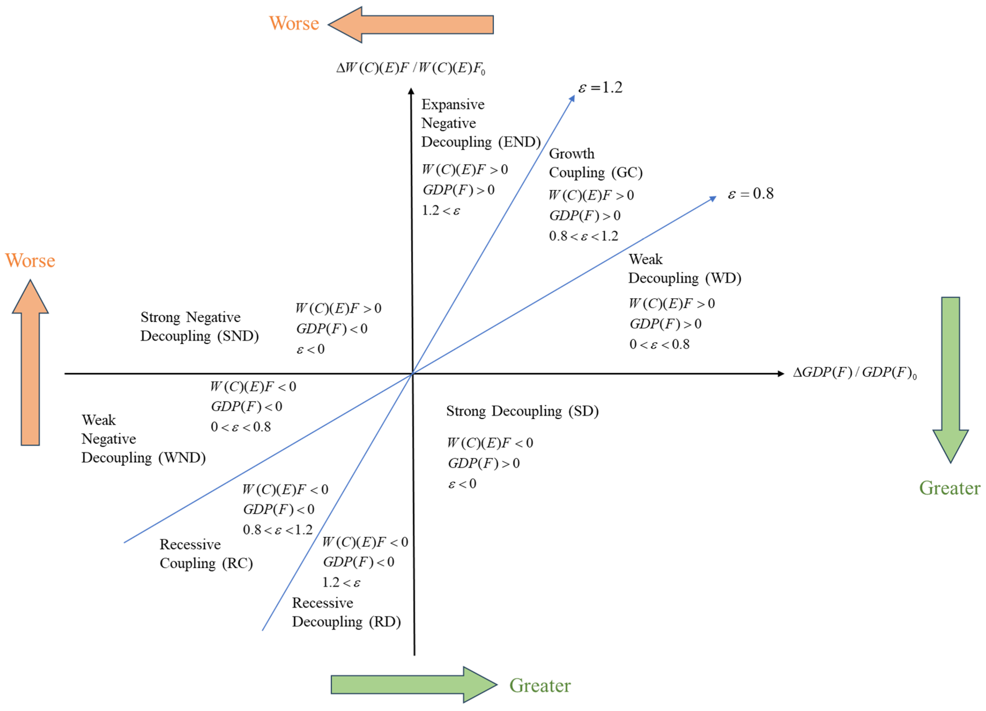
2.5. “Water–Carbon–Ecological” Footprint Drivers Tapio Decoupling Analysis

In this study, the Tapio model is employed. According to the variations of the decoupling index, the decoupling status is classified into eight distinct states: Weak decoupling (WD), growth connection (GC), expansive negative decoupling (END), strong negative decoupling (SND), weak negative decoupling (WND), recession connection (RC), recessionary decoupling (RD), and strong decoupling (SD) [17,18]. Figure 1 elaborates on other details. On this basis, the drivers with the highest contributions to water, carbon, and ecological footprints are analyzed for decoupling respectively. The calculation expressions of this model are as follows:

The calculation formula of the Tapio decoupling elasticity coefficient between water footprint and economic effect factors is as follows:

$${\epsilon }_1={\displaystyle \frac{\Delta WF/W{F}_0}{\Delta GDP/GD{P}_0}}={\displaystyle \frac{(W{F}_t-W{F}_0)/W{F}_0}{(GD{P}_t-GD{P}_0)/GD{P}_0}}$$

(34)

The calculation formula of the Tapio decoupling elasticity coefficient between carbon footprint and agricultural production scale factors is presented as follows:

$${\epsilon }_2={\displaystyle \frac{\Delta CF/C{F}_0}{\Delta F/F_0}}={\displaystyle \frac{(C{F}_t-C{F}_0)/C{F}_0}{(F_t-F_0)/F_0}}$$

(35)

The calculation formula for the Tapio decoupling elasticity coefficient between the ecological footprint and economic effect factors is as follows:

$${\epsilon }_3={\displaystyle \frac{\Delta EF/E{F}_0}{\Delta GDP/GD{P}_0}}={\displaystyle \frac{(E{F}_t-E{F}_0)/E{F}_0}{(GD{P}_t-GD{P}_0)/GD{P}_0}}$$

(36)

where ${\epsilon }_1$ denotes the decoupling index between the water footprint and economic effect factors, ${\epsilon }_2$ represents the decoupling index between the carbon footprint and agricultural production scale factors, ${\epsilon }_3$ indicates the decoupling index between the ecological footprint and economic effect factors, GDP stands for the gross domestic product (CNY) of the construction industry, and $F$ represents the grain production quantity.

Figure 1. Diagram of the Division Results of Decoupling States.

Figure 1. Diagram of the Division Results of Decoupling States.

2.6. Data Sources

The research objects of this paper are 11 provinces and cities in the YREB (Shanghai, Jiangsu, Zhejiang, Anhui, Jiangxi, Hubei, Hunan, Chongqing, Sichuan, Yunnan, Guizhou), and the research period is from 2002 to 2017. We collected relevant indicator data from the China Statistical Yearbook (2002–2017), the China Energy Statistical Yearbook (2002–2017), the China Urban Construction Statistical Yearbook (2002–2017), the China Rural Statistical Yearbook (2002–2017), the China Health Statistics Yearbook (2002–2017), the China Water Statistics Yearbooks (2002–2017), and provincial statistical yearbooks.

3. Results and Discussion

3.1. Spatio-Temporal Evolution Characteristics of the Footprint Family

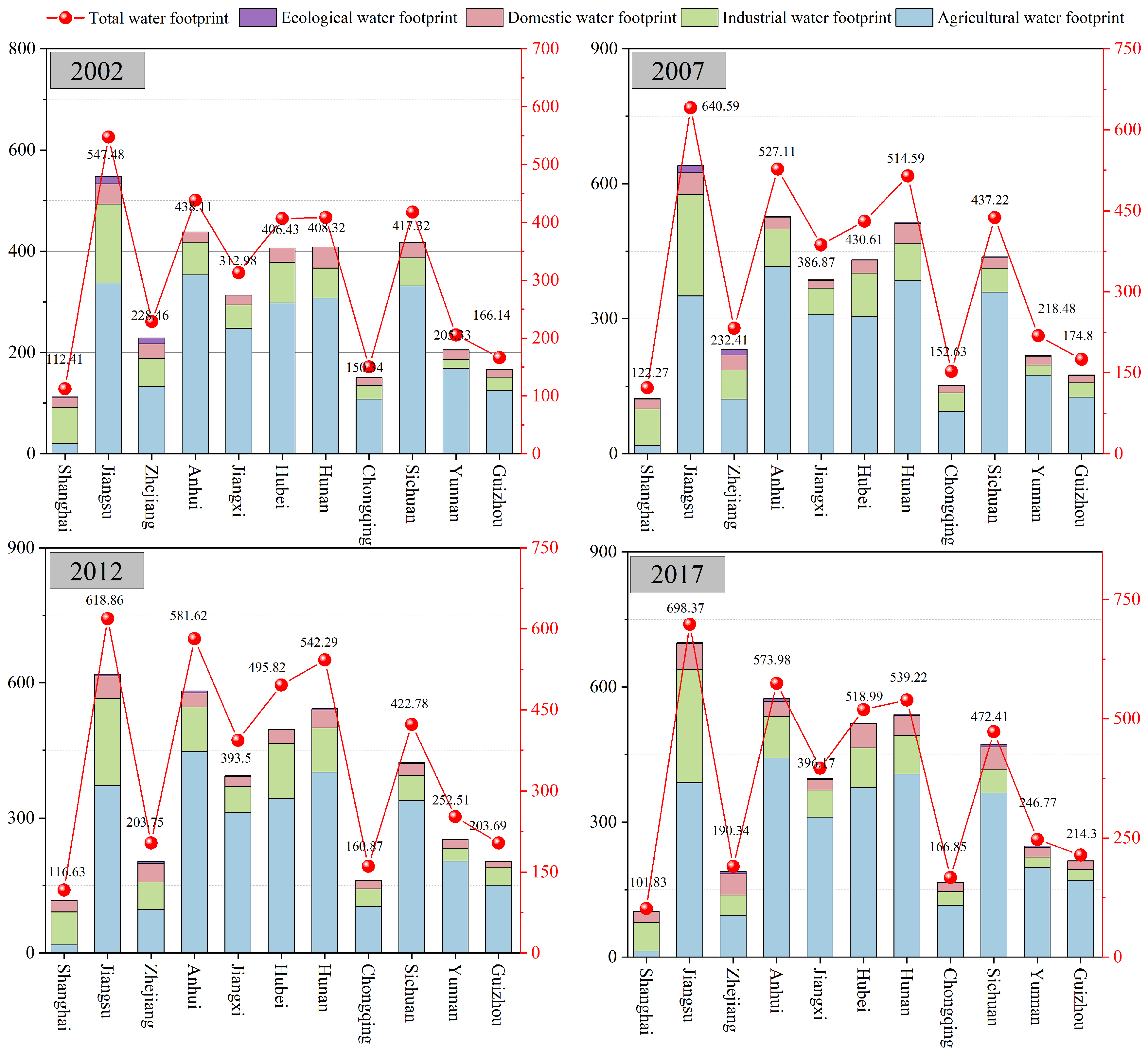
3.1.1. Spatio-Temporal Characteristics of the Water Footprint

The total water footprints of Jiangsu Province from 2002 to 2017 were 54.748 billion m³, 64.059 billion m³, 61.886 billion m³, and 69.837 billion m³, respectively, with a total of 250.23 billion m³, all being the highest among the eleven provinces and municipalities. The total water footprints of Shanghai from 2002 to 2017 were 11.241 billion m³, 12.227 billion m³, 11.663 billion m³, and 10.183 billion m³, respectively, with a total of 45.314 billion m³, all being the lowest among the eleven provinces and municipalities. The industrial water footprint had the highest proportion in Shanghai’s water footprint. Except for Shanghai, the agricultural water footprint had the highest proportion in the other ten provinces and municipalities. The total water footprint of the YREB from 2002 to 2007 was 1534.265 billion m³. Among them, the agricultural water footprint was 1074.812 billion m³, accounting for a proportion of 70.05%, which was the highest. The ecological water footprint was 12.601 billion m³, accounting for a proportion of 0.82%, which was the lowest. The annual data and comprehensive water footprint results of 11 provinces and cities in the YREB from 2002 to 2017 are shown in Figure 2.

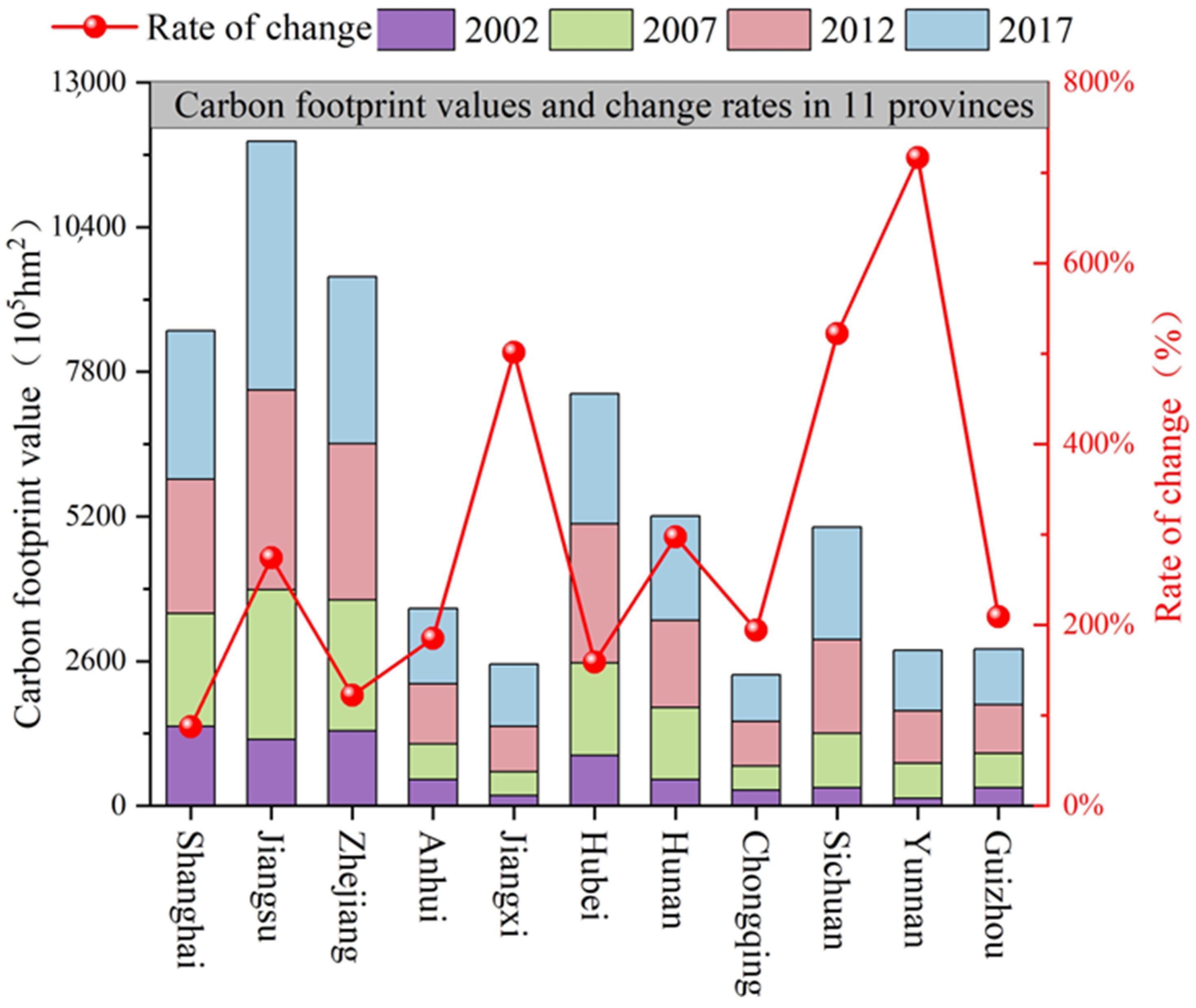
3.1.2. Spatio-Temporal Evolution Characteristics of Carbon Footprint

The carbon footprint values of Jiangxi Province in 2002, 2007, 2012, and 2017 were 1.8591 million hm², 4.2975 million hm², 8.0947 million hm², and 11.1826 million hm², respectively, all being the lowest among the eleven provinces and municipalities. The carbon footprint value of Shanghai in 2002 was 14.252 million hm², being the highest among the eleven provinces and municipalities. The carbon footprint values of Jiangsu Province in 2007, 2012, and 2017 were 26.8964 million hm², 35.8556 million hm², and 44.7363 million hm², respectively, all being the highest among the eleven provinces and municipalities. The total carbon footprint of the YREB in 2002 and 2007 was 70.6943 million hm² and 137.7194 million hm², with the change rates being 94.81% and 38.44%, respectively. In 2012, the total carbon footprint was 190.6603 million hm², and the change rate was 38.44%. In 2017, the total carbon footprint was 217.6549 million hm², and the change rate was 14.16%. The annual data change rate and spatial change trend of the total carbon footprint of 11 provinces and cities in the YREB from 2002 to 2017 are shown in Figure 3.

3.1.3. Spatio-Temporal Evolution Characteristics of Ecological Footprint

In 2002, the per capita EF of Shanghai was 2.014 hm² per person, the highest among the eleven provinces and municipalities, while that of Guizhou Province was 0.962 hm² per person, the lowest among them. In 2007, 2012, and 2017, the per capita EF of Hubei Province was 2.353 hm² per person, 3.212 hm² per person, and 3.162 hm² per person, respectively, all the highest among the eleven provinces and municipalities. In 2007 and 2012, the per capita EF of Chongqing was 1.28 hm² per person and 1.71 hm² per person, respectively, both the lowest among the eleven provinces and municipalities. In 2017, the per capita EF of Sichuan Province was 1.024 hm² per person, the highest among the eleven provinces and municipalities. The inter-annual data and spatial change trend of the per capita 3D ecological footprint of 11 provinces and cities along the YREB from 2002 to 2017 are shown in Figure 4.

3.2. Decomposition of Driving Factors of the Footprint Family

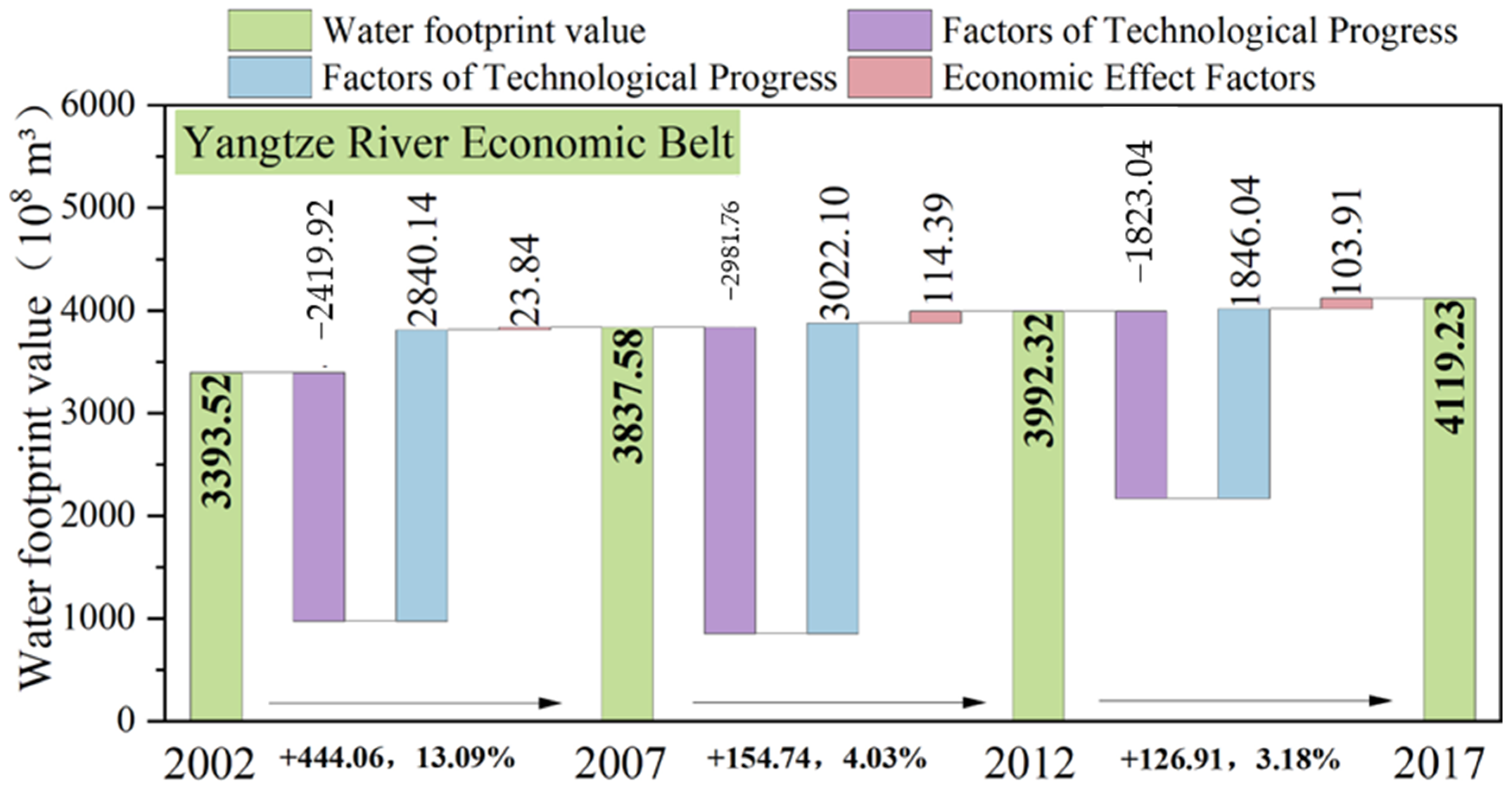
3.2.1. Decomposition of Driving Factors of the Water Footprint by LMDI

It can be seen from the figure that the economic effect factor has the most significant promoting effect on the water footprint of the eleven provinces and municipalities, with an average contribution of approximately 23.358 billion m³ from 2002 to 2017. The main reason is that with the rapid economic development, the amount of cooling water and process water required for industrial production, as well as the irrigation water required for agricultural production, has increased significantly.

Additionally, economic development has driven the improvement of water resource management and protection regulations, further promoting the rational utilization and protection of water resources. The technological progress factor has the most significant inhibitory effect on the water footprint of the eleven provinces and municipalities, with an average contribution of approximately −21.893 billion m³ from 2002 to 2007. This is mainly due to the significant improvement in water resource utilization rate as technology grows in various regions. As can be seen from the figure, the more significant the promoting effect of the economic effect factor, the more obvious the inhibitory effect of the water consumption intensity factor. This is mainly because economic development has increased water demand while technological progress has improved water utilization and reduced water consumption. From 2002 to 2007, the contributions of the economic effect factor and the water consumption intensity factor in Jiangsu Province were 50.71 billion m³ and −42.83 billion m³, respectively. From 2012 to 2017, the contributions of the economic effect factor and the water consumption intensity factor in Anhui Province were 27.155 billion m³ and −28.678 billion m³, respectively, both being the highest among the eleven provinces and municipalities. From 2002 to 2017, the population size factor had a promoting effect on the water footprint in economically developed regions such as Shanghai, Jiangsu, and Zhejiang, but the promoting effect was limited.

The average contribution in Shanghai was approximately 1.428 billion m³. This is mainly because, with the growth of the population size, the water consumption for production, living, and ecological purposes has increased significantly, and the inflow of population in economically developed regions is relatively high. From 2012 to 2017, the population size factor had a promoting effect on the water footprint of the eleven provinces and municipalities, with an average contribution of approximately 0.945 billion m³. The analysis results of water footprint driving factors of 11 provinces and cities in the YREB from 2002 to 2017 are shown in Figure 5.

It can be observed from the figure that the economic effect factor has the most significant promoting impact on the water footprint of the YREB. The average contribution was 284.014 billion m³ from 2002 to 2007, 302.21 billion m³ from 2007 to 2012, and 184.6 billion m³ from 2012 to 2017. The water consumption intensity factor has the most significant inhibitory effect on the water footprint of the YREB, with average contributions of −241.99 billion m³ from 2002 to 2007, −298.17 billion m³ from 2007 to 2012, and −182.3 billion m³ from 2012 to 2017. The population scale factor has a consistently promoting effect on the water footprint of the YREB, with average contributions of 23.8 billion m³ from 2002 to 2007, 114.3 billion m³ from 2007 to 2012, and 103.9 billion m³ from 2012 to 2017. The analysis results of driving factors of the water footprint in the YREB from 2002 to 2017 are shown in Figure 6.

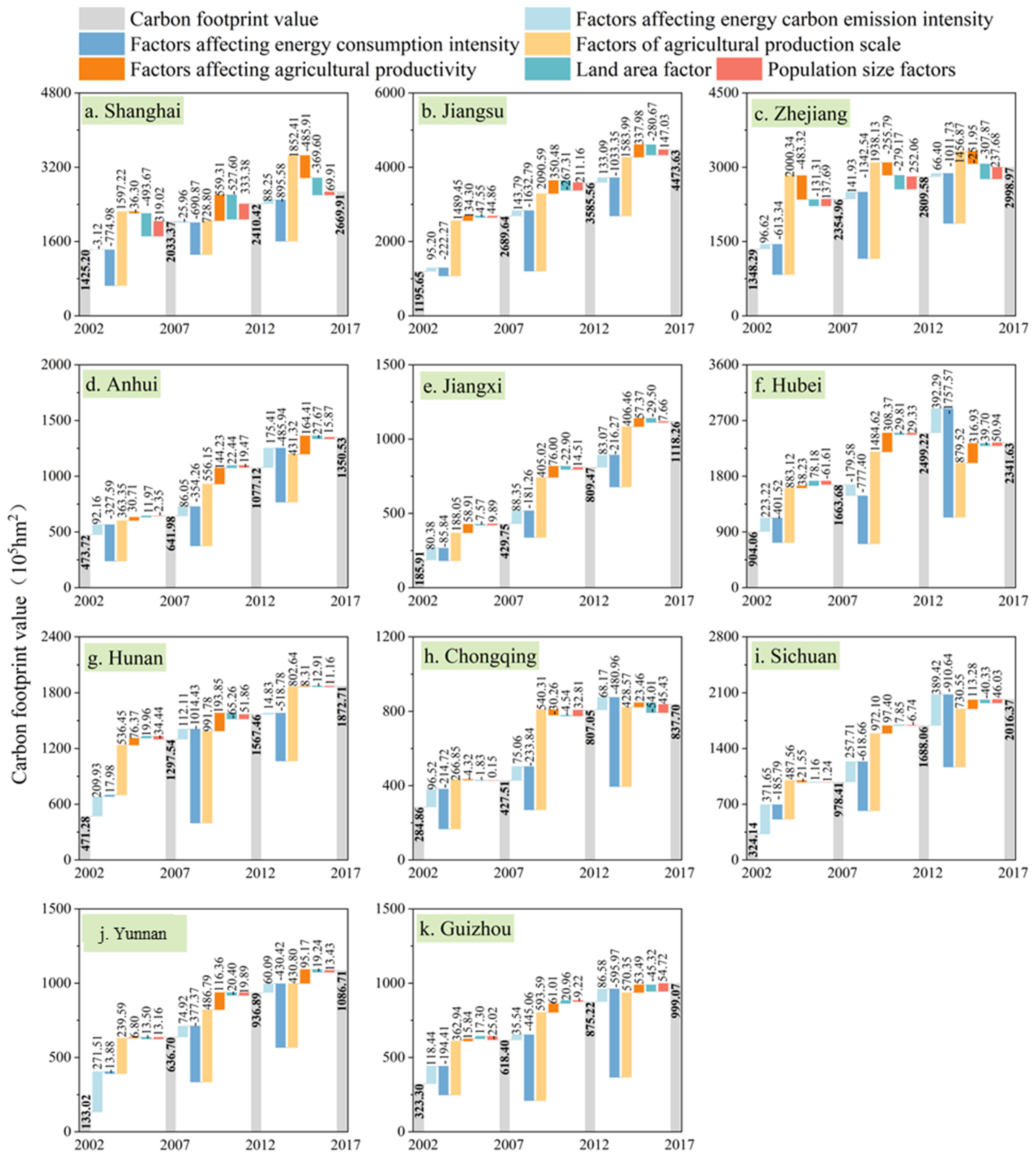
3.2.2. Decomposition of Driving Factors of Carbon Footprint by LMDI

As revealed in the figure, the factors of energy carbon emission intensity and agricultural production efficiency typically enhance the carbon footprint value of the eleven provinces and municipalities. From 2012 to 2017, the average contribution of the energy carbon emission intensity factor and the agricultural production efficiency factor to the carbon footprint of the eleven provinces and municipalities was 1.4159 million hm² and 393,200 hm², respectively. The agricultural production scale factor has the most significant promoting effect on the carbon footprint of the eleven provinces and municipalities, with an average contribution of approximately 8.7201 million hm² from 2002 to 2017. This is mainly because the average grain production in the eleven provinces and municipalities increased from 17.7421 million tons in 2002 to 21.915 million tons in 2017.

The excessive use of mechanical diesel and pesticides in the grain production process would raise the carbon footprint value of each province and municipality. The technological progress factor has the most significant inhibitory effect on the carbon footprint of the eleven provinces and municipalities. With the promotion of clean energy, enterprises can reduce their reliance on high-carbon emission technologies and adopt low-carbon or zero-carbon emission technologies. The advancement of carbon reduction technologies can significantly reduce carbon emissions during the production process, thereby exerting an inhibitory effect on the carbon footprint. From 2012 to 2017, the population scale factor had a promoting effect on the carbon footprint of the eleven provinces and municipalities. This is mainly because the population of the eleven provinces and municipalities increased from 583 million to 601 million.

The expansion of the population size requires meeting living needs such as food and transportation, and the satisfaction of these needs often requires the consumption of a large amount of energy such as fossil fuels, thereby leading to an increase in greenhouse gas emissions and ultimately an increase in the carbon footprint. From 2012 to 2017, the land area factor had an inhibitory effect on the carbon footprint of the eleven provinces and municipalities. This is mainly because intensified year by year, and the areas of water bodies, forest land, and other land types have expanded year by year, thereby absorbing a large amount of carbon dioxide and exerting an inhibitory effect on the carbon footprint. The carbon footprint driving factors of 11 provinces and cities in the YREB from 2002 to 2017 are shown in Figure 7.

From 2002 to 2017, the factors of energy carbon emission intensity, agricultural production scale, and population scale all exerted a promoting effect on the carbon footprint value of the YREB, with their average contribution values being 13.4002 million hm², 95.9209 million hm², and 6.7067 million hm², respectively. Consequently, the factor of agricultural production scale was the most crucial driving factor for the carbon footprint value of the YREB. The factors of technology and land area both had an inhibitory effect on the carbon footprint value of the YREB, with their average contribution values being −63.4068 million hm² and −9.8648 million hm², respectively. From 2002 to 2007, the factor of agricultural production efficiency inhibited the carbon footprint value of the YREB, with an average contribution value of 6.2305 million hm².

3.2.3. Decomposition of Driving Factors of Ecological Footprint by LMDI

The structural factor and the economic factor have a remarkable promoting effect on the ecological footprint of the eleven provinces and municipalities. From 2002 to 2017, the average contributions of the structural factor and the economic factor were 1.6796 million hm² and 6.6676 million hm², respectively. This is mainly because, as the economy develops and people’s living standards rise, the consumption structure is constantly changing. People’s demand for food, housing, etc. is increasing, and at the same time, they pay more attention to the improvement of living quality and environmental protection awareness. However, this transformation of the consumption structure also leads to a large consumption of natural resources and environmental damage.

The technological factor has a significant inhibitory effect on the ecological footprint of the eleven provinces and municipalities. From 2002 to 2017, the average contribution of the technological factor was −7.0385 million hm². This is mainly because, with the continuous advancement of technology, the wide application of efficient energy-saving technologies, clean energy technologies, and resource recycling technologies can significantly improve the utilization efficiency of resources, reduce the waste and pollutants generated in the production process, and thereby reduce the consumption of natural resources and environmental damage.

The population scale factor usually promotes the ecological footprint of the eleven provinces and municipalities. From 2012 to 2017, it had a promoting effect on the ecological footprint value of the eleven provinces and municipalities, with an average contribution of 363,200 hm². This is mainly because, with the growth of the population and the acceleration of the urbanization process, the urban population scale expands rapidly. This not only increases the demand for resources such as land, water, and energy in cities but also aggravates urban environmental pollution and ecological damage.

From 2002 to 2017, the structural factors, economic factors, and population scale factors all exerted a promoting effect on the ecological footprint value of the YREB, with their average contribution values being 18.4753 million hm², 73.3441 million hm², and 3.093 million hm², respectively. Hence, the economic factor was the most significant driver of the ecological footprint value of the YREB. The technological factor had an inhibitory effect on the carbon footprint value of the YREB, with an average contribution value of −77.4238 million hm².

Through multi-dimensional decomposition analysis, this study systematically reveals the driving mechanism and spatio-temporal evolution of the water–carbon–ecological footprint in the YREB. The study found that technological progress showed significant sectoral heterogeneity: The water consumption per unit output in the agricultural sector decreased by 28% due to the upgrading of irrigation technology, but the regional differences were significant (35% in Jiangsu vs. 18% in Guizhou). The utilization rate of recycled water in the industrial sector has improved significantly since 2012, but there is still a 15–20% technology gap in the upper and middle provinces. The structural nature of the economic drive shows that the contribution of the secondary industry to the carbon footprint shows an “inverted U-shaped” curve, in which the energy industry is always the largest contributor (42–49%), while the equipment manufacturing industry’s share surged from 15% to 27%.

It is worth noting that the driving force shows obvious spatial and temporal heterogeneity: After 2012, the technology substitution effect of the Yangtze River Delta urban agglomeration is significant, and the decline rate of water consumption per unit GDP exceeds the national average by 40%. The midstream provinces are still in the “investment-driven” stage, and their economic contribution continues to be 15–20 percentage points higher than the technology inhibition effect. In the upstream region, the land carbon sequestration function was significantly enhanced due to ecological compensation policies (carbon sequestration increased by 3.2% per year).

The study also identified the impact of several key policy nodes, such as a 2.1-fold increase in the diffusion rate of industrial water-saving technologies after the implementation of water resource management regulations in 2011. These findings not only quantified the relative importance of different driving factors but also revealed their operating conditions and change thresholds, providing a scientific basis for the formulation of differentiated regional environmental management policies.

It is suggested that subsequent studies can be combined with enterprise-level micro data to further verify the micro mechanism of macro decomposition results and establish dynamic optimization models to predict the evolution of driving effects under different policy scenarios.

Based on the independent analysis of the existing driving factors, this study further reveals the complex interaction mechanism among the driving factors during the evolution of the “W-C-E” footprint in the YREB. It is found that the relationship between economic effect and technological progress factors is not simply linear but presents dynamic synergy-antagonistic transformation characteristics: In the accelerated industrialization stage (2002–2012), the promotion effect of economic expansion on water resource consumption was partially offset by technological progress, and the two formed an “efficiency catch-up” antagonistic relationship.

In the transformation and upgrading stage (2012–2017), economic structure optimization and technological innovation turn into a synergistic relationship, showing that each 1% increase in total factor productivity can reduce the water footprint intensity of economic growth by 0.38%. It is particularly noteworthy that there is a significant spatial coupling between population agglomeration effect and technology diffusion efficiency. Every 10% increase in population density in the Yangtze River Delta urban agglomeration will increase the diffusion rate of water-saving technology by 6.2% through innovation factor agglomeration. This “scale-innovation” positive feedback mechanism is weak in the central and western regions.

The study also found that policy regulation played a key role in regulating the interaction of driving factors. For example, the implementation of ecological compensation policies transformed the antagonistic relationship between economic growth and carbon sink function into a synergistic relationship in the middle and upstream regions. These findings break through the limitation of traditional single factor analysis and build a “drive–response–feedback” system analysis framework, which provides a new theoretical support for the formulation of sustainable development policies based on multi-factor coordination. In future studies, the complex network method can be used to further quantify the threshold of nonlinear interaction between different driving factors and its spatial transfer effect.

3.3. Decoupling Analysis of Footprint Family Driving Factors

3.3.1. Decoupling Analysis of Water Footprint (Tapio)

As shown in Figure 8, during the research period, two decoupling states emerged: WD and SD, with the occurrence frequencies of 24 and 9 times, respectively. During the study period, most provinces exhibited a trend of transitioning from a weak decoupling state to a strong decoupling state. Specifically, all were in the weak decoupling state from 2002–2007, the number of strong decoupling states increased to four from 2007–2012, and further rose to five from 2012–2017.

At the provincial level, Shanghai, Zhejiang, Anhui, Hunan, and Yunnan were in the WD state from 2002–2007 and all shifted to the SD state after 2012. Jiangxi, Hubei, Chongqing, and Guizhou remained in the WD state throughout the research period. Sichuan and Jiangsu changed from the SD state to the WD state in 2012. During the study period, all areas in the YREB were in a decoupling state, but the decoupling index decreased from 0.166 to 0.0585.

In 2017, the GDP of the YREB was CNY 37,380.6 billion, an increase of 8.0% compared to the previous year, accounting for 45.2% of the national total, an increase of 0.5 percentage points compared to the previous year. The rapid economic development simultaneously drove the adjustment of the industrial structure and technological progress. With the advancement of technology and the improvement of management levels, the water resource utilization efficiency in fields such as agricultural production and industrial manufacturing in the YREB could be significantly enhanced. This implies that, while the economy was growing, the consumption of water resources did not increase synchronously and might even have declined, thereby strengthening the decoupling trend between the water footprint and the economy.

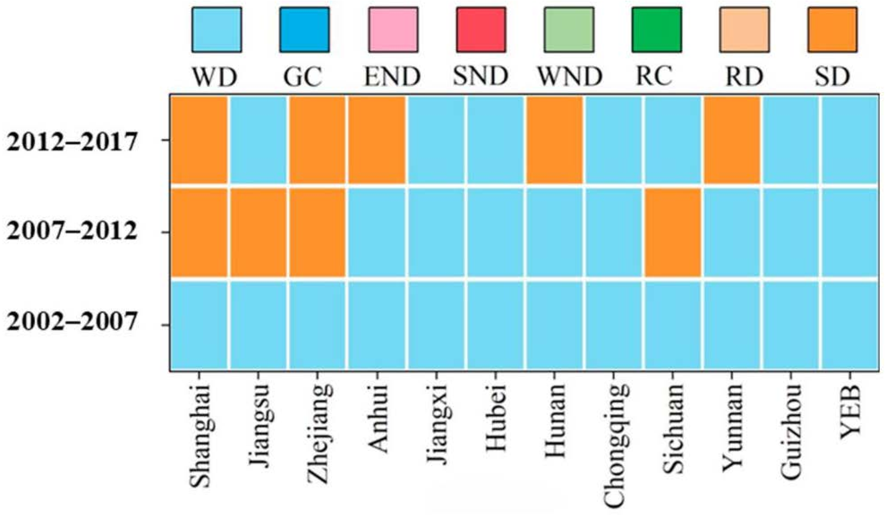
3.3.2. Decoupling Analysis of Carbon Footprint

As shown in Figure 9, during the research period, four decoupling states emerged: GC, END, SND, and SD, with the occurrence frequencies being 1, 23, 8, and 1, respectively. During the study period, the decoupling index of the majority of provinces witnessed reductions to varying degrees. Specifically, the average decoupling index was 18.67 from 2002–2007, −21.14 from 2007–2012, and 6.8 from 2012–2017.

Sichuan Province transformed from the SND state to the END state from 2012 to 2017. From 2012–2017, Shanghai, Zhejiang, and Hubei were in the SND, SND, and SD states, respectively, while the remaining provinces were all in the END state. Throughout the research period, the YREB was in the END state, but its decoupling index decreased from 23.96 to 2.166.

This is mainly attributed to the enhancement of agricultural production management levels, including efficient resource allocation and meticulous management of the production process, which contributes to the reduction of carbon emissions. During the production process, enterprises and farmers can decrease carbon emissions while ensuring production output by measures such as optimizing irrigation systems and reducing the usage of chemical fertilizers and pesticides. On the other hand, the transformation of the economic growth mode in the YREB, from the traditional growth mode dependent on resource consumption to a more green and sustainable development model, has lowered the correlation between carbon emissions in agricultural production and economic growth.

Figure 9. Decoupling results of carbon footprint driving factors in eleven provinces and cities along the YREB.

Figure 9. Decoupling results of carbon footprint driving factors in eleven provinces and cities along the YREB.

3.3.3. Tapio Decoupling Analysis of Ecological Footprint

As shown in Figure 10, during the research period, all eleven provinces and municipalities were in a state of weak decoupling. However, the decoupling indices of most provinces and municipalities, such as Shanghai, Jiangsu, and Jiangxi, declined to varying extents. The average decoupling index value for the eleven provinces and municipalities from 2002 to 2007 was 0.187, and from 2012 to 2017, it was 0.109, with a decrease rate of 41.7%.

At the provincial level, the decoupling index of Shanghai declined from 0.305 to 0.051, with a decline rate amounting to 83.27%, while that of Hubei decreased from 0.174 to 0.0088, with a decline rate reaching 94%. The decoupling index values of Jiangsu, Jiangxi, Hunan, Chongqing, Sichuan, Yunnan, and Guizhou all witnessed varying degrees of decrease. The decoupling index value of Zhejiang rose from 0.0559 to 0.0726, and that of Anhui increased from 0.0439 to 0.0694. During the study period, the entire YREB remained in a WD state, but its decoupling index dropped from 0.169 to 0.114, with a decrease rate of 32.54%.

This is primarily attributed to the intensified efforts in ecological environment restoration and protection in the YREB. Through measures such as implementing ecological restoration projects and strengthening the construction of nature reserves, various provinces and cities have enhanced the stability and self-restoration capacity of the ecosystem. The implementation of these measures is conducive to reducing the damage of economic activities to the ecological environment, thereby further promoting the decoupling of ecological footprints from economic factors.

This study analyzed the decoupling status of the W-C-E footprint in the YREB and revealed the important implications of different decoupling types for the formulation of sustainable development policies. It is found that the emergence of SD indicates the absolute separation of economic growth and environmental pressure, which mainly occurs in the downstream areas where the industrial structure is advanced (the tertiary industry accounts for >55%) and green technology innovation is prominent. While the WD state shows the improvement of relative efficiency, the absolute value of environmental pressure is still increasing, suggesting the need to strengthen total control. In particular, the study identified significant gradient characteristics: The downstream regions with strong decoupling should focus on institutional innovation (such as the construction of carbon trading markets), the midstream provinces with weak decoupling should promote the green transformation of traditional industries (such as reducing the water consumption of the steel industry by 18%), and the upstream regions with negative decoupling expansion should establish ecological compensation mechanisms (compensation standards up to 65% of the value of ecosystem services).

By assessing the gap between decoupling dynamics and SDG targets, we found that provinces with strong water footprint decoupling have achieved SDG6.4 ahead of schedule, but the negative decoupling status of carbon footprint expansion indicates that an additional 21% reduction is still needed to achieve SDG13. Based on this, the study puts forward differentiated policy recommendations: Implement green GDP assessment for strongly decoupled regions, implement an industry energy efficiency “leader” system for weakly decoupled regions, and set resource and environmental red lines for negatively decoupled regions.

The study also found that, after the implementation of the Outline of the YREB Development Plan, the inter-provincial decoupling speed difference was reduced by 18%, suggesting the subsequent establishment of a cross-provincial decoupling index compensation mechanism, and the decoupling status should be included in the core indicators of green development demonstration zone evaluation. These findings provide a quantitative basis for the formulation of the implementation rules of the Yangtze River Protection Law and indicate that the goal of carbon neutrality must be achieved through the coordination of technological innovation and institutional innovation, from relative decoupling to absolute decoupling, which will be a key challenge for the green transformation of the YREB in the next decade.

Figure 10. Decoupling results of ecology footprint driving factors in eleven provinces and cities along the YREB.

Figure 10. Decoupling results of ecology footprint driving factors in eleven provinces and cities along the YREB.

4. Conclusions

4.1. Conclusions

This study has established a research framework for the driving factors of footprint families based on Kaya–LMDI–Tapio, quantitatively assessed the systematic correlations among footprint families in the study area and the contribution of driving factors, and analyzed the decoupling status between footprint families and the main driving factors. Based on the calculation results, targeted sustainable development strategies were put forward. The main findings of the study are summarized as follows:

(1) The total water footprint of the YREB from 2002 to 2007 was 1534.265 billion m³. Among them, the agricultural water footprint was 1074.812 billion m³, accounting for 70.05%, the highest proportion. The ecological water footprint was 12.601 billion m³, accounting for 0.82%, the lowest proportion. The total carbon footprint in 2002 and 2007 was 70.6943 million hm², with a change rate of 94.81%. The total carbon footprint in 2012 was 190.6603 million hm², with a change rate of 38.44%. The total carbon footprint in 2017 was 217.6549 million hm², with a change rate of 14.16%. The per capita EF of Sichuan Province in 2017 was 1.024 hm² per person, the highest among the eleven provinces.

(2) The main driving factors of the water footprint and ecological footprint in the eleven provinces are economic effect factors, with average contributions of 23.358 billion m³ and 6.6676 million hm² from 2002 to 2017, respectively. The most significant inhibitory effect on the water footprint and ecological footprint is attributed to the factor of technological progress, with average contributions of −21.893 billion m³ and −7.0385 million hm², respectively. The factor of agricultural production scale has the most significant promoting effect on the carbon footprint, with an average contribution of approximately 87.201 million hm² from 2002 to 2017. The most significant inhibitory effect on the carbon footprint in the eleven provinces is attributed to the factor of technological progress.

(3) During the research period, the decoupling results of water footprint from economic factors in most provinces exhibited a tendency to shift from weak decoupling to strong decoupling. The decoupling indices of carbon footprint from the agricultural production scale in the eleven provinces decreased to varying extents. The decoupling results of the ecological footprint from economic factors in the eleven provinces were all weak decoupling, but the decoupling indices in most provinces such as Shanghai, Jiangsu, and Jiangxi declined to different degrees.

(4) There are still limitations in this study, which can be improved in future studies. In terms of research methods, the Kaya–LMDI decomposition assumes that each driving factor has a linear relationship, which may ignore the nonlinear effect of resource consumption. The Tapio decoupling model also provides only static analysis and cannot reflect long-term dynamic feedback mechanisms. Moreover, the study uses aggregated data at the regional level, which conceals the spatial heterogeneity of urban and rural areas, upstream and downstream in the basin. In addition, factors such as macroeconomic fluctuations, climate change impacts, and environmental policies implemented after 2007 were not included in the analytical framework. Finally, the assessment of each footprint type (water, carbon, ecology) is relatively independent, and its synergistic pressure cannot be quantified, and the ecological footprint index is still insufficient in the characterization of biodiversity loss and other issues.

4.2. Policy Recommendations

This study has constructed an analysis framework for the driving factors of the footprint family, laying a foundation for researchers to calculate the realization of sustainable development in different provinces and regions and providing new insights for policy customization. It holds practical significance and potential for international promotion. In light of the current development status of China’s industries, the following policies are required for China to achieve sustainable social development:

(1) To effectively address the issue of economic factors being the main drivers of water and ecological footprints and to curb decoupling, policy suggestions include strengthening the management and planning of water and ecological resources, promoting the development of water-saving technologies and water-saving industries, and optimizing the industrial structure and layout to reduce resource consumption and environmental pollution [19]. Simultaneously, it is necessary to enhance policy guidance and market mechanism construction, raise public awareness of water conservation and environmental protection, and actively draw on international experience and participate in global governance to jointly promote sustainable development and achieve a favorable decoupling between resource consumption and economic growth [20].

(2) To alleviate the problem of agricultural production scale being the main driver of the carbon footprint and to suppress decoupling, comprehensive measures are proposed: Promoting organic agriculture and optimizing farming methods, reducing the use of chemical fertilizers and pesticides, and enhancing mechanization efficiency; adjusting the planting structure and improving livestock husbandry management, selecting low-carbon crop varieties, and reducing methane emissions from livestock; strengthening the management of agricultural waste and converting it into biomass energy or organic fertilizer; researching, developing, and promoting low-carbon agricultural technologies, such as carbon capture and storage; rationally planning the scale of agricultural production to avoid excessive expansion [21].

(3) Based on the analysis results of the “W-C-E” footprint decoupling in the YREB, this study proposes a set of precise policy system with watershed characteristics. For the downstream YREB, it is proposed to implement the “zero-carbon park” upgrade plan, requiring the park to achieve full coverage of photovoltaic energy storage by 2025, and establish a green technology trading center of the YREB, focusing on promoting the market-oriented application of advanced technologies such as water treatment membrane technology. For the midstream provinces, it is proposed to carry out the “green recycling of traditional industries” project, mandatory implementation of waste heat recovery systems and intelligent water recycling devices in the steel and nonferrous industries, and to set up a special transformation fund of CNY 20 billion to support the recycling transformation of chemical parks. For upstream regions, the operation mechanism of an “ecological bank” has been innovatively designed, ecological assets such as forest carbon sinks have been securitized, and precision agriculture technologies such as variable fertilization by drones have been promoted. In terms of technological innovation, it is suggested to establish an innovation consortium of the Yangtze River Academy of Water Sciences to research low-cost seawater desalination technology, lay out hydrogen energy infrastructure along the river, and develop green shale gas mining technology. The system innovation level includes three major measures: The establishment of decoupling index financial transfer payment mechanism, pilot cross-provincial water rights transaction, and the establishment of the Yangtze River ecological prosecutor system.

References

1. Ciupek, B.; Brodzik, Ł.; Frąckowiak, A. Research on Carbon Footprint Reduction During Hydrogen Co-Combustion in a Turbojet Engine. Energies 2024, 17, 5397. [Google Scholar] [CrossRef]
2. Deng, L.; Xu, Y.; Xue, F.; Pei, Z. Mining interpretable fuzzy If-Then linguistic rules from energy and economic data to forecast CO [formula omitted] emissions of regions in China. Energy 2024, 313, 133631. [Google Scholar] [CrossRef]
3. Guo, J.; Wei, Z.; Xie, X.; Ren, J.; Zhou, H. Dynamic change and driving force of natural capital in Qinghai Province based on the three-dimensional ecological footprint, China. Ecol. Indic. 2022, 145, 109673. [Google Scholar] [CrossRef]
4. Lai, Z.; Li, L.; Huang, M.; Tao, Z.; Shi, X.; Li, T. Spatiotemporal evolution and decoupling effects of sustainable water resources utilization in the Yellow River Basin: Based on three-dimensional water ecological footprint. J. Environ. Manag. 2024, 366, 121846. [Google Scholar] [CrossRef]
5. Lerpiniere, J.D.; Wilson, C.D.; Velis, A.C. Official development finance in solid waste management reveals insufficient resources for tackling plastic pollution: A global analysis of two decades of data. Resour. Conserv. Recycl. 2025, 212, 107918. [Google Scholar] [CrossRef]
6. Liu, Q.; Chen, T.; Zhang, N.; Ye, Z.; Jiang, K.; Lin, Z.; Gao, Y.; Guo, Y.; Weng, A. Green energy meets urban agriculture: Unveiling the carbon reduction potential of Rooftop Agrivoltaics. J. Clean. Prod. 2024, 480, 144110. [Google Scholar] [CrossRef]
7. Ma, X.; Liu, C.; Niu, Y.; Zhang, Y. Spatiotemporal pattern and prediction of agricultural blue and green water footprint scarcity index in the lower reaches of the Yellow River Basin. J. Clean. Prod. 2024, 437, 140691. [Google Scholar] [CrossRef]
8. Tian, L.; Chai, J.; Zhang, X.; Pan, Y. Spatiotemporal evolution and driving factors of China’s carbon footprint pressure: Based on vegetation carbon sequestration and LMDI decomposition. Energy 2024, 310, 133299. [Google Scholar] [CrossRef]
9. Niccolucci, V.; Galli, A.; Reed, A.; Neri, E.; Wackernagel, M.; Bastianoni, S. Towards a 3D National Ecological Footprint Geography. Ecol. Model. 2011, 222, 2939–2944. [Google Scholar] [CrossRef]
10. Wang, L.Z.; Tao, F.; Leng, J.H.; Wang, Y.-H.; Zhou, T. multi-scale analysis on sustainability and driving factors based on three-dimensional ecological footprint: A case study of the Yangtze River Delta region, China. J. Clean. Prod. 2024, 436, 140596. [Google Scholar] [CrossRef]
11. Lin, C.; Li, X. Carbon peak prediction and emission reduction pathways exploration for provincial residential buildings: Evidence from Fujian Province. Sustain. Cities Soc. 2024, 102, 105239. [Google Scholar] [CrossRef]
12. Liu, Q.; Li, F.; Dong, S.; Cheng, H.; Liang, L.; Xia, B. Spatial-temporal heterogeneity of sustainable development goals and their interactions and linkages in the Eurasian continent. Sustain. Prod. Consum. 2024, 52, 151–165. [Google Scholar] [CrossRef]
13. Sun, D.; Cai, S.; Yuan, X.; Zhao, C.; Gu, J.; Chen, Z.; Sun, H. Decomposition and decoupling analysis of carbon emissions from agricultural economic growth in China’s YREB. Environ. Geochem. Health 2022, 44, 2987–3006. [Google Scholar] [CrossRef]
14. Wang, M.; Huang, X.; Dong, Y.; Song, Y.; Wang, D.; Li, L.; Qi, X.; Lin, N. Spatiotemporal drivers of agricultural non-point source pollution: A case study of the Huang-Huai-Hai Plain, China. J. Environ. Manag. 2024, 370, 122606. [Google Scholar] [CrossRef] [PubMed]
15. Xie, P.; Shu, Y.; Sun, F.; Li, P. Decoupling economic development from carbon emissions: Insights from Chinese provinces. Energy 2024, 308, 133008. [Google Scholar] [CrossRef]
16. Yang, X.; Fan, Y.; Yao, Y.; Tan, M.; Xu, H. Temporal and spatial variations of land carbon loss caused by animal-sourced foods consumption in China and the driving factors. Environ. Impact Assess. Rev. 2024, 109, 107644. [Google Scholar] [CrossRef]
17. Zhang, L.; Li, H.; Yang, L.; Du, X.; Zhou, Y.; Sun, G.; Liu, J. Carbon footprints of centralized and decentralized food waste utilization pathways. Renew. Sustain. Energy Rev. 2025, 208, 115040. [Google Scholar] [CrossRef]
18. Zhang, Y.; Bian, Z.; Guo, X.; Wang, C.; Guan, D. Strategic land management for ecosystem Sustainability: Scenario insights from the Northeast black soil region. Ecol. Indic. 2024, 168, 112784. [Google Scholar] [CrossRef]
19. Zhao, D.; Wang, W.; Ji, X.; Wu, P.; Zhuo, L. Nitrogen cycling and associated grey water footprint in croplands under different irrigation practices. J. Clean. Prod. 2024, 480, 144081. [Google Scholar] [CrossRef]
20. Zhao, Y.; Gao, G.; Zhang, J.; Yu, M. Impact of carbon tax on green building development: An evolutionary game analysis. Energy Policy 2024, 195, 114401. [Google Scholar] [CrossRef]
21. Zhou, W.; Chi, Y.; Tang, S.; Hu, Y.; Wang, Z.; Zhang, X. The evolution analysis of low-carbon power transition strategies and carbon emission decoupling based on carbon neutrality target. Energy 2024, 311, 133298. [Google Scholar] [CrossRef]
Figure 2. Results of Comprehensive Water Footprint of the YREB by Province and Autonomous Region from 2002 to 2017 (Unit: 100 million m3).
Sustainability 17 03645 g002
Figure 3. Total Carbon Footprint of the Eleven Provinces and Municipalities in the YREB (Unit: 10,000 hm2).
Sustainability 17 03645 g003
Figure 4. Per Capita Three-Dimensional Ecological Footprint of the Eleven Provinces and Municipalities in the YREB (Unit: hm2/person).
Sustainability 17 03645 g004
Figure 5. Result Diagram of Contribution Degree of Driving Factors of Water Footprint in Different Provinces and Autonomous Regions of the YREB.
Sustainability 17 03645 g005
Figure 6. Result Diagram of the Contribution Degree of Driving Factors of Water Footprint in the YREB.
Sustainability 17 03645 g006
Figure 7. Result Diagram of the Contribution Degree of Driving Factors of Carbon Footprint by Province and District in the YREB.
Sustainability 17 03645 g007
Figure 8. Decoupling results of water footprint driving factors in eleven provinces and cities along the YREB. Note: The color interpretation in Figure 8 includes the color interpretation in Figure 8, Figure 9 and Figure 10.
Sustainability 17 03645 g008