Modeling Intervehicle Spacing for Safe and Sustainable Operations on Two-Lane Roads

Abstract

This paper examines the essential role of intervehicle spacing on two-lane rural roads, highlighting its significance for traffic safety and management. Recent technological advancements have enabled the precise positioning of vehicles on highways through video recordings and image processing techniques. However, these systems are less applicable to rural roads due to the absence of extensive sensor networks. This study bridges this gap by proposing a simulation-based model to evaluate the probability density of intervehicle spacing under varying traffic conditions. The simulation model integrates macroscopic traffic flow theories with microscopic car following models, simulating intervehicle spacings over a considerable highway segment. Calibration and validation were conducted using data from a two-lane road in Northern Italy. The simulation results identify key characteristics of spacing distribution, including positive skewness (i.e., a longer tail toward higher values), high kurtosis (a peaked distribution with frequent extreme values), non-zero minimum values, and autocorrelation at high traffic densities (indicative of platooning behavior). The Pearson type III distribution was determined to be the most suitable fit for the experimental data. Thus, future research should focus on parameter estimation for the Pearson type III distribution to further understand intervehicle spacing under varying traffic conditions and to expand applications to various road types and traffic scenarios.

1. Introduction

The measurement of intervehicle spacing is a fundamental element of traffic analysis for characterizing traffic conditions, driving behaviors, and road safety, as it directly relates to vehicle density [1]. This, in turn, affects traffic characteristics and the levels of service on uninterrupted flow facilities, such as multilane highways and freeways [2,3].

Thus, understanding proper intervehicle spacing is a key factor for developing traffic models that enhance highway safety, support sustainability initiatives for safer roads, set minimum and recommended distances, and enforce necessary safety standards. According to existing research, a significant number of traffic accident investigations reveal that rear-end collisions are a major type of traffic accident and make up a significant share of all crashes [4,5,6]. These collisions typically occur when the leading vehicle suddenly decelerates or when the following vehicle accelerates more rapidly than expected. The primary causes include driver inattention, unintentional close following due to misjudging deceleration needs, and intentional aggressive tailgating [7].

In this context, it is essential to analyze and accurately characterize driver behaviors in terms of intervehicle spacing to specify and calibrate rear-end collision models and test mitigation strategies. Recent technological advancements now allow the precise tracking of vehicle positions using video recording and image processing methods that previously relied on aerial photography [8]. In contrast, inter-arrival times, speeds, and volumes can be easily recorded at transverse highway sections using various sensor-based measurement systems, which have advanced alongside traffic flow research [9].

Recent studies demonstrate a growing interest in applying machine learning (ML) and deep learning (DL) to traffic flow analysis, particularly for modeling intervehicle spacing and estimating safe following distances. Several notable studies include deep learning approaches for car following behavior classification [10], LSTM-based vehicle trajectory prediction [11], hybrid clustering–deep learning models for vehicle acceleration estimation [12], and computer vision methods for spacing estimation in agricultural contexts [13]. Additionally, research leveraging ensemble regression [14], super-deep learning for automated driving [15], and CNN-LSTM models for lane change behavior prediction [16] further confirm the relevance of AI technologies in this domain.

To address limitations in detecting vehicle positions and spacing along a lane, indirect methods are often used to estimate vehicle density. These derive from instantaneous vehicle volume and average speed measurements at a transverse section or from temporal headways and point-based speed monitoring [17]. Sensors positioned at a fixed point collect data on two consecutive vehicles to generate real-time intervehicle spacings. These spacings are essential for analyzing vehicle interactions and platoon formation based on standard research thresholds [18]. The resulting density values are local to a small highway segment (elementary stretch) at the observation section. Extending these to longer road stretches assumes stationary traffic conditions over a given period. Therefore, only average values can represent spacing, limiting probabilistic insights over entire highway segments [19]. Alternative methods apply sensors, like GPS, LiDAR, radar, or infrared, over short segments—typically in experimental settings—to estimate intervehicle spacing. These devices measure real-time spacing but are confined to the localized areas where they are installed [17].

Given these challenges, the direct measurement of intervehicle spacing and density has historically been difficult. However, advancements in image and video analysis technologies now enable the extraction of traffic parameters from camera recordings [20]. On instrumented highways, such as motorways, the availability of video systems enables the real-time monitoring of larger segments and the direct measurement of spacing and density at specific times. Such data are crucial for traffic management and control [21] and play a key role in modern Intelligent Transport Systems and Smart Road applications [22]. Accurately predicting and modeling intervehicle spacings support traffic control strategies, including speed limits and lane management [23].

Despite this progress, current research highlights that much of the technology is still primarily applicable to well-instrumented highways. Studies such as those by [24] demonstrate ML and DL models’ performance for parking prediction—an area closely related to intervehicle spacing. Meanwhile, methodologies integrating multiple algorithms (e.g., ensemble regression) for accurate V2V distance prediction [14] show promising capabilities for implementation beyond traditional infrastructures. These models represent significant progress but also underscore the need for simpler, cost-effective solutions suited for rural or under-equipped roads.

The importance of studying intervehicle spacing, particularly their probabilistic distributions, is clear. This research responds by addressing the under-representation of spacing (as opposed to temporal headways) in traffic modeling. It identifies suitable probabilistic distributions for modeling vehicle distances. While image and sensor systems allow data collection on equipped motorways, this capability does not extend to most two-lane rural roads that make up national traffic networks [25].

Two-lane roads serve as a critical link between urban and interurban traffic systems, connecting higher-level infrastructures, such as roads, railways, ports, and airports, to local markets and vice versa. Enhancing the functionality [26] and safety [27] of these roads is essential for sustainable corridor development. However, their geometric complexity and low funding make sensor installations impractical. In such contexts, analyzing intervehicle spacing distributions using probabilistic models under varying traffic conditions can support practical safety and sustainability improvements.

This study proposes a simulation-based method to evaluate the probability density of intervehicle spacing on a two-lane rural road with no overtaking. Unlike approaches that rely on sensor-rich environments or high-resolution visual data, the model simulates intervehicular spacing over an extended highway segment using macroscopic and microscopic traffic models integrated with probabilistic tools. It operates under varying traffic conditions, including different levels of the initial traffic volume and density. Calibrated on monitored road sections in Italy, this approach distinguishes itself by offering a realistic, innovative, and cost-efficient solution that supplements recent research advancements while addressing the specific safety and sustainability challenges of rural road networks.

This paper is structured as follows: Section 2 details the methodology for analyzing intervehicle spacing distributions using a simulation model that integrates a macro approach (a Fundamental Diagram analysis) with a micro approach (the car following model) for single-lane traffic without overtaking. It also describes vehicle generation functions based on temporal headways and arrival speeds, varying with the average hourly arrival flow rate. Calibration and validation are performed using data from a two-lane road in Northern Italy, for which the geometric characteristics and axis alignment have already been recognized and identified [28]. Section 3 provides an analysis of the results, highlighting the variations in the experimental spatial headways distribution due to variations in the simulated arrival flow rate and the resulting average density. It also discusses the findings in relation to the statistical characteristics of spatial headways and explores suitable probabilistic models for their representation, while Section 4 presents the study’s main conclusions.

2. Materials and Methods

2.1. Spacing Simulation Model for a Single-Lane Traffic Stream

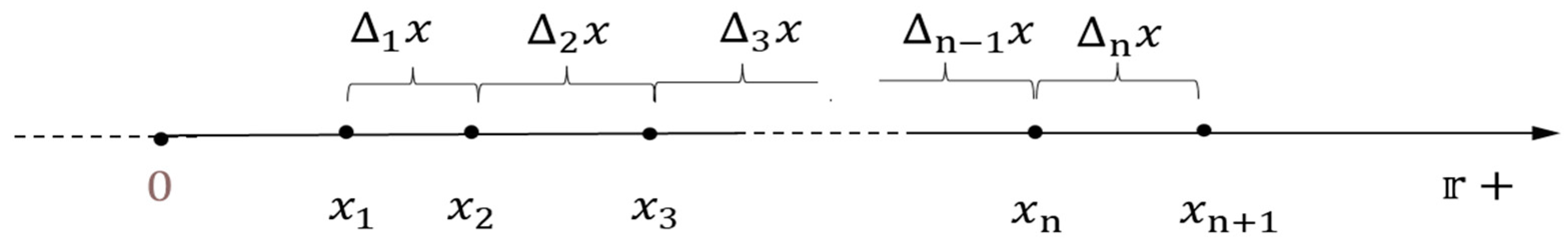
We consider an infinitely long stretch of a two-lane highway, focusing on one direction of travel, where only light vehicles are permitted, and overtaking is completely restricted. This allows for a single vehicle class analysis. The defined segment is represented by the half-line, $\mathbb{r}+$, oriented in the direction of travel, with the origin, O, marking the initial cross-section of the modeled highway segment.

Figure 1 shows a sequence of increasing random abscissas, $x_1$, $x_2$, …, $x_n$, representing vehicle positions along $\mathbb{r}+$. The spacing between consecutive vehicles is given by ${\mathrm{\Delta }}_{i}x$ = $x_{i+1}-x_i$ for $i$ = 1, 2, …, $n$, indicating mutual distances. The vehicle sequence can be expressed in terms of spacing alone as $x_1$; $x_2=x_1+{\mathrm{\Delta }}_{1}x$; $x_3=x_1+{\mathrm{\Delta }}_{1}x+{\mathrm{\Delta }}_{2}x$…, without explicitly considering individual positions.

The Spacing Simulation Model analyzes spatial distancing probability distributions within a single-lane traffic stream, examining their variations with different hourly flow rates and average densities. It consists of two main components: the Vehicle Generation Model (VGM) and the Vehicle Interaction Model (VIM).

The VGM defines vehicle entry parameters at the origin point of $\mathbb{r}+$, representing a single-lane traffic stream of indefinite length. It includes the Temporal Headway Distribution Model (THDM) and the Initial Speed Distribution Model (ISDM):

• The THDM assigns temporal headways between consecutive vehicles, based on a probabilistic distribution, to ensure realistic traffic-flow simulations.
• The ISDM defines initial vehicle speeds using a simplified stochastic Fundamental Diagram [1], capturing variations in driver behavior and vehicle performance at the entry point.

The VIM governs how vehicles interact after entering the traffic stream. It comprises two sub-models, namely the First Vehicle Speed Pattern (FVSP) and the car following model (CFM):

• The FVSP sets the speed behavior of the lead vehicle, influencing the dynamics of all the following vehicles.
• The CFM simulates how trailing vehicles adjust their speeds and distances based on the preceding vehicle, incorporating reaction times and safe following distances to prevent collisions.

This structured approach enables a detailed analysis of traffic flow dynamics and spatial dynamics, facilitating the study of how varying traffic densities and flow rates impact overall traffic behavior. The following sections define the simulation model, with a focus on each of the four sub-models.

2.1.1. Temporal Headway Distribution Model (THDM)

In assigning temporal headways to each vehicle at O, the THDM differentiates between conditioned and non-conditioned vehicles [18]. Specifically, conditioned vehicles are restricted to speeds lower than their desired speed due to the inability to overtake the preceding vehicle, while non-conditioned vehicles have a desired speed equal to or lower than that of the preceding vehicle. By probabilistically identifying the status of each following vehicle (conditioned vs. non-conditioned), a mixed-type headway distribution model is applied. The probability distribution of time headways, $f\left(\tau \right)$, is expressed as $f\left(\tau \right)=\phi ·g\left(\tau \right)+(1-\phi )·h\left(\tau \right)$ [19], where $\phi$ represents the probability of a conditioned vehicle, with its time headway probability distribution, $g\left(\tau \right)$; and $(1-\phi )$ represents the probability of a non-conditioned vehicle, with its time headway probability distribution, $h(\tau$). This formulation separates constrained (following) and free (non-following) conditions, enabling a more precise characterization of time headway distributions in the traffic stream. The transition from non-congested to congested conditions, shifting from $h\left(\tau \right)$ to $g\left(\tau \right)$, can be modeled using established approaches from the literature [29,30], such as Buckley’s Semi-Poisson Model [31], Cowan’s M3 and M4 models [32], and Branston’s Generalized Queuing Model [33], among others [26]. In this simulation, we adopted the TLR-SPM model by [26], which defines $\phi$ based on ${\Gamma }_C\left(Q\right)$, which is a function representing the proportion of constrained (non-free) vehicles in the traffic stream as a function of flow rate $Q$.

The ${\Gamma }_C\left(Q\right)$ function can be estimated for the specific lane type under consideration using a data-driven approach [26]. For the $h\left(\tau \right)$ and $g\left(\tau \right)$ functions, the general criteria and references outlined in Section 2 apply. Consistent with previous definitions, the simulation model assumes, for conditioned vehicles (in platoons), a Pearson type III (three-parameter Gamma) distribution for headways, with a defined ${\tau }_{\mathrm{*}}$, considering $k$ and $\lambda$ as functions of the hourly flow rate, $Q$ (or its equivalent in vehicles per second, $q$) [34]. Similarly, for unconditioned vehicles (that are free from interactions), the model considers a shifted exponential headway distribution, with a minimum headway threshold of ${\tau }_{\mathrm{*}}={\tau }_{\mathrm{s}}$. Thus, the probability distribution is as follows:

$$g\left(\tau \right)={\displaystyle \frac{\lambda }{\mathrm{\Gamma }\left(\tau \right)}}·{\left[\lambda \left(\tau -{\tau }_{\mathrm{*}}\right)\right]}^{k-1}exp\left\{-\lambda \left(\tau -{\tau }_{\mathrm{*}}\right)\right\}\hspace{1em}for \tau \ge {\tau }_{\mathrm{*}}$$

(1)

with $k=f\left(Q\right)$ and $\lambda =k·q$, where $q=Q/3600$. For unconditioned vehicles, since the shifted exponential distribution is a special case of the Pearson type III distribution, the function $h\left(\tau \right)$ can be derived from Equation (1) by setting ${\tau }_{\mathrm{*}}={\tau }_{\mathrm{s}}$, $k=1$, and $\lambda =q$.

2.1.2. Initial Speed Distribution Model (ISDM)

In assigning the initial speed, $V_i(t=0)$, to each vehicle, $i$ (i.e., its speed in O when it is generated by the simulation), the ISDM considers a normal distribution for both conditioned and non-conditioned vehicles as follows:

$$f\left(V\right)={\displaystyle \frac{1}{\sigma \sqrt{2\pi }}}·exp\left\{-{\displaystyle \frac{1}{2}}{\left({\displaystyle \frac{V-\mu }{\sigma }}\right)}^2\right\}$$

(2)

with $\mu =\mu \left(Q\right)$ and $\sigma =\sigma \left(Q\right)$, which can be estimated based on real data for situations of the type under consideration (for example, as we will see in the next section, considering a macroscopic model of a Fundamental Diagram (FD) for the function describing the variation of the mean value and an interval regression model for the function of the standard deviation), to obtain a simplified yet convenient form of a stochastic (namely, Gaussian) Fundamental Diagram [1,35,36].

2.1.3. First Vehicle Speed Pattern (FVSP)

The First Vehicle Speed Pattern (FVSP) defines the speed trajectory of the first vehicle ($i=0$) entering the simulation at t $=0$. The model describes speed variations along the lane without distinguishing whether the vehicle is conditioned or not. The speed trend is expressed as a function of $V_0\left(x\right)$, where speed varies with position $x$ along $\mathbb{r}+$. Since the simulation operates with constant time steps ($∆t=1$ s), the speed profile can be implemented as a step function, $V_0\left(t\right)$, at one-second intervals. This speed trend can be freely defined to analyze specific effects, such as variations in the desired speed, along the path. The initial speed, $V_0\left(0\right)$, is assigned according to the Initial Speed Distribution Model (ISDM).

2.1.4. Car Following Model (CFM)

Following the sequence of the sub-models, when a vehicle $(i=1,\dots ,n$) is generated, its temporal headway relative to the preceding vehicle $(i-1)$ is assigned based on the THDM; its entry speed, $V_i(t=0)$, is determined by the ISDM; the speed trend of the first vehicle ($i=0$) is set by the FVSP. At this stage, the car following model (CFM) governs interactions between consecutive vehicles $(i$ and $i+1$, for $i=0, 1,\dots ,n)$.

Car following models are essential in traffic simulation and transportation engineering, providing insights into individual vehicle behavior in response to preceding vehicles [37]. These models describe the dynamic relationship between vehicles, focusing on variables such as speed, acceleration, and intervehicle distance [38]. They simulate real-world traffic dynamics using phenomenological assumptions [39], often structured around the fundamental relationship, Response = Sensitivity · Stimulus, first proposed by [40,41], where acceleration is the response, and the speed difference between vehicles acts as the stimulus [42,43].

In this study, the car following model (CFM) adopted is the one formulated by [44,45], commonly known as the General Motors (GM) model, certainly one of the most well-known stimulus-based models [46]. In the GM model, the sensitivity, denoted as $\alpha$, is not constant but varies as a function of the following vehicle’s travel speed and the spacing between vehicles. For a discrete time simulation with an updating time, $∆t$, the sensitivity, $\alpha$, is expressed as

$$\alpha \left(t\right)={\overline{\alpha }}_{l,m}·{\displaystyle \frac{{V_{i+1}\left(t-∆t\right)}^m}{{\left(x_i\left(t-\delta t\right)-x_{i+1}\left(t-\delta t\right)\right)}^l}}={\alpha }_{l,m}(t)$$

(3)

where $V_i\left(t\right)$ is the instantaneous speed of the i-th vehicle at time t, $∆t$ is the updating time interval in the discrete simulation, $\delta t$ is the reaction time of the driver, $x_i$ is the travelling distance of the i-th vehicle from O at time t, $m$ is the speed exponent, $l$ is the spacing exponent, and ${\overline{\alpha }}_{l,m}$ the sensitivity coefficient dependent on $m$ and $l$. The following equations can be used to describe the mathematical form of the GM model:

$$V_i\left(t\right)=V_i\left(t-∆t\right)+a_i\left(t-∆t\right)·∆t$$

(4)

$$x_i\left(t\right)=x_i\left(t-∆t\right)+V_i\left(t-∆t\right)·∆t+{\displaystyle \frac{1}{2}}{a}_i\left(t-∆t\right)·{(∆t)}^2$$

(5)

$$a_{i+1}\left(t\right)={\alpha }_{l,m}\left(t\right)·\left[V_i\left(t-∆t\right)-V_{i+1}\left(t-∆t\right)\right]$$

(6)

where $a_i\left(t\right)$ is the instantaneous acceleration rate of the $i$-th vehicle at time $t$, and coefficients ${\alpha }_0$, $m$, and $l$ allow for calibrating and particularizing the model, considering $l$ between [−1, 4] and $m$ between [−2, 2].

Considering that $∆t=1$ s, we can conveniently set the reaction time as $\delta t=∆t=1$, simplifying the application of Equations (4)–(6) in a discrete time simulation:

$$V_i\left(t\right)=V_i\left(t-1\right)+a_i\left(t-1\right)$$

(7)

$$x_i\left(t\right)=x_i\left(t-1\right)+V_i\left(t-1\right)+{\displaystyle \frac{1}{2}}{a}_i\left(t-1\right)$$

(8)

$$a_{i+1}\left(t\right)={\alpha }_0·{\displaystyle \frac{{V_{i+1}\left(t-1\right)}^m}{{\left(x_i\left(t-1\right)-x_{i+1}\left(t-1\right)\right)}^l}}·\left[V_i\left(t-1\right)-V_{i+1}\left(t-1\right)\right]$$

(9)

It has been shown that by assigning precise values to coefficients $m$ and $l$, and assuming a steady state hypothesis, many macroscopic traffic laws, also known as Fundamental Diagram (FD) functions, can be directly derived from the non-linear GM car following model [1]. Thus, for different ($m$, $l)$ pairs, a corresponding macroscopic relationship, $V=V\left(Q\right)$, can be identified, establishing a link between microscopic vehicle interactions and the macroscopic behavior of the entire traffic stream. The values of $m$ and $l$ are selected to align with the function $\mu =\mu \left(Q\right)$, which represents the average speed in the ISDM model. From this perspective, the base sensitivity coefficient, ${\alpha }_0$, can be estimated, taking on a specific interpretation based on the selected $(m$, $l)$ pair and its associated macroscopic traffic law [45].

2.2. The Simulation Algorithm

Following the structure of the four models outlined in Section 2.1, the simulation algorithm computes vehicle spacing under different flow rates, $Q$. The key computational steps are

• Flow rate definition: A specific flow rate, $Q$, is selected, ranging from 100 to 1300 veh/h in increments of 100 veh/h. For each flow rate, 100 Monte Carlo (MC) simulations [47,48] are performed.
• The generation of the first vehicle ($i$ = 0): The first vehicle, $i=0$, is placed at the origin, O, with an initial speed, $V_{i=0}(t=0)$. In each simulation, a random number, ${RND}_0$, is generated using Monte Carlo sampling. The initial speed, $V_{i=0}(t=0)$, follows a Gaussian distribution with a mean of ${\mu }_0=\mu \left(Q\right)$ and a standard deviation of ${\sigma }_0=\mu \left(Q\right)$, estimated from real data. The vehicle’s trajectory, $x_0\left(t\right)$, is updated over time using FVSP, with discrete steps, $∆t=1$ s.
• The generation of the following vehicles (i = 1 to 100): Vehicle spacing is assigned based on the THDM: the proportion of the following vehicles is determined using ${\Gamma }_C\left(Q\right)$, estimated from real data. A random number, $RND1$, is generated: if $RND1<1-{\Gamma }_C\left(Q\right)$, a non-following vehicle is generated, otherwise a following vehicle is generated. For non-following vehicles, the headway, ${\tau }_{\mathrm{i}}$, is sampled from a shifted exponential distribution with ${\tau }_{\mathrm{s}}$ and $\mathrm{\lambda }=\mathrm{Q}/3600$. For the following vehicles, the headway, ${\tau }_{\mathrm{i}}$, is sampled from a three-parameter Gamma distribution, with ${\tau }_{*}$, $\mathrm{\lambda }=\mathrm{k}·\mathrm{Q}/3600$, and $k=k\left(Q\right)$.
• Position and speed calculation for each vehicle (i = 1 to 100): Position $x_i\left(t\right)$ is updated at each discrete time step, $∆t=1$ s, considering its headway, ${\tau }_{\mathrm{i}}$, relative to the previous vehicle, $\mathrm{i}-1$; its initial speed $V_i(x=0)$, sampled from a Gaussian distribution, with ${\mu }_i=\mu \left(Q\right)$ and ${\sigma }_i=\mu \left(Q\right)$ (the same as in step 2); its speed evolution $V_i(x,t)$, based on the GM car following model (CFM), using $\delta t=∆t=1 \mathrm{s}$, $l\in$ [−1,4], $m\in$ [−2,2], and ${\overline{\alpha }}_{l=1,m=0}$, estimated from real data.

The simulation model evaluates traffic flows ranging from 100 veh/h to 1300 veh/h in increments of 100 veh/h (i.e., 100, 200, 300, …, 1100, 1200, 1300 veh/h). For each hourly flow rate, 100 vehicular sequences were simulated, each consisting of 100 vehicles entering the simulation at the origin O of $\mathbb{r}+$. Vehicle entry follows temporal headways assigned by the THDM, initial speeds determined by the ISDM, mutual interactions governed by the CFM, and speed trends over time defined by the FVSP. The model assumes a single vehicle class and a no-overtaking rule. The specifications of the four sub-models are based on real traffic data collected at a road section that aligns with the model’s assumptions. In total, the simulation generates 130,000 vehicles, tracking their movement along $\mathbb{r}+$ from O over an indefinite lane length under the defined traffic conditions. For each series of 100 simulated vehicles, the following key data points are extracted:

• Temporal headways, ${\tau }_{\mathrm{i}}(x=0)$ ($i=1,\dots ,100$). The time intervals between consecutive vehicles at the origin, O (used for validation against the experimental headway distribution from the reference road section).
• Initial speeds, $V_{\mathrm{i}}(x=0)$ ($i=1,\dots ,100$). The speeds at which vehicles enter the simulation at O (compared with the experimental speed distribution from real-world data).
• Vehicle spacing, $s_{\mathrm{i}}(t=t^{*})$ ($i=1,\dots ,100$), includes the average vehicle length (4.5 m). It is defined as ${∆x}_i=x_{i-1}\left(t^{*}\right)-x_i\left(t^{*}\right)$, representing the distance to the preceding vehicle at the time, $t^{*}$, when the 100th vehicle is generated at O.

2.3. The Specification, Calibration, and Validation of the Simulation Model on a No-Passing, Rural, Two-Lane Road

The data used for specifying, calibrating, and validating the model were obtained from the same monitoring section described in [26]. The monitoring section was equipped with 24,165 GHz Doppler radar instruments installed on both sides of the carriageway. The site was a straight, level segment of a two-lane rural road in Northern Italy, characterized by a speed limit of 90 km/h, a no-transit rule for heavy vehicles over 3.5 tons, and a no-overtaking rule for all vehicle categories. The monitoring session lasted 24 h in both travel directions, recording approximately 28,000 vehicles under normal-working-day conditions, with no atmospheric disturbances or accidents affecting the traffic flow.

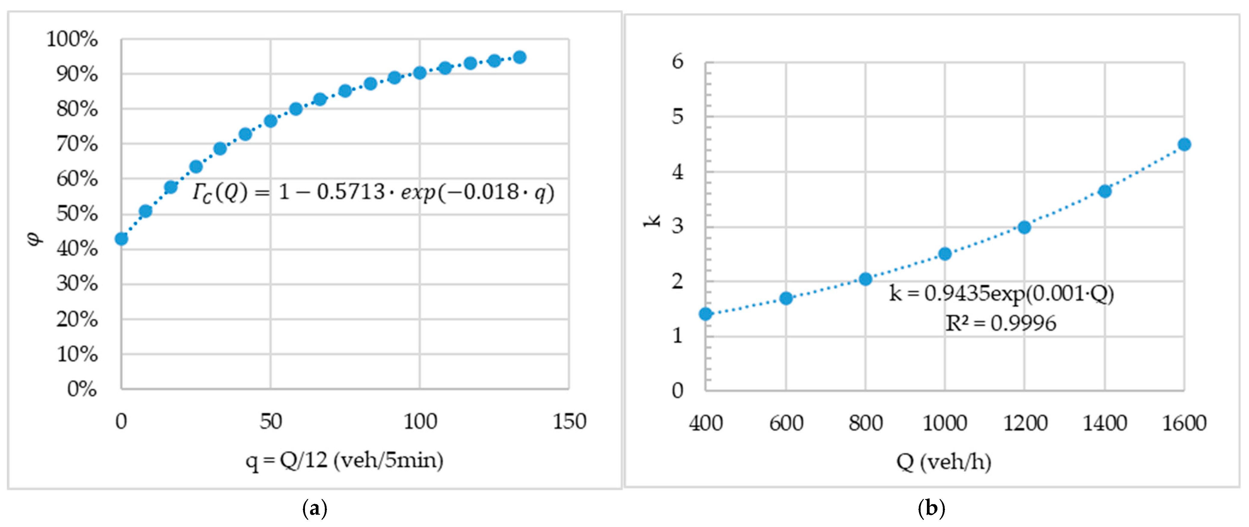
The first step in the modeling chain is defining the vehicle generation process through headway sampling, governed by the Temporal Headway Distribution Model (THDM). This requires both the specification of the function $\phi \left(Q\right)$, which segments hourly traffic into conditioned (following) and unconditioned (free) vehicles, and the probability distributions $g\left(\tau \right)$ and $h\left(\tau \right)$ definition for these two vehicle categories. The function ${\Gamma }_C\left(Q\right)=1-0.5713·exp(-0.018·Q/12)$ was calibrated by [26] for the same monitoring section (Figure 2a) and determinates the proportion of following vehicles. For non-free vehicles, in line with [19], a Pearson type III distribution (three-parameter Gamma) was used with ${\tau }_{\mathrm{*}}=0.5$ s and $\lambda =k·Q$, and the relationship $k=f\left(Q\right)$ was defined based on [19,49] as $k=0.9435·exp(0.001·Q)$. Similarly, for free vehicles, a shifted exponential distribution was used, with $\lambda =Q$ and ${\tau }_{\mathrm{*}}={\tau }_{\mathrm{s}}=4$ s [18,19].

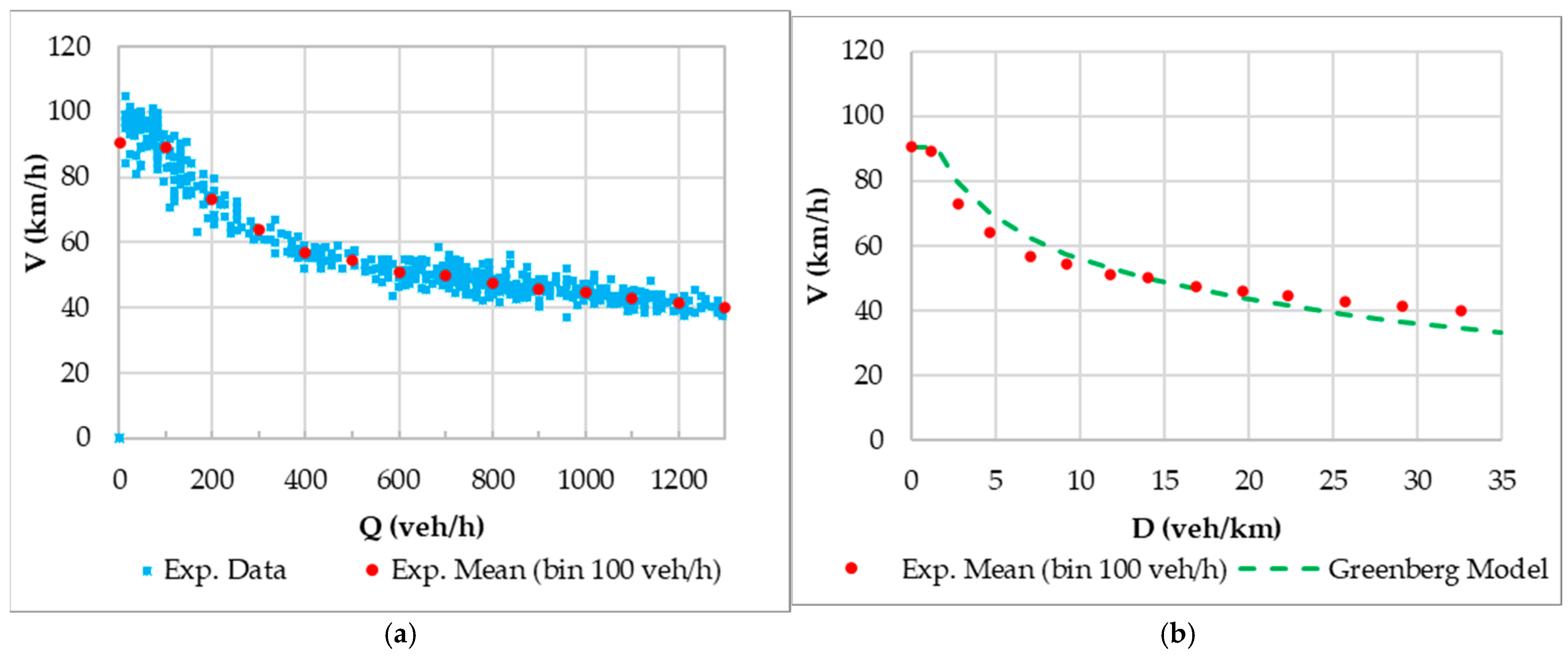
To define the Fundamental Diagram (FD) model for ${\mu }_i=\mu \left(Q\right)$, the hourly flow data and 5 min average speed data were analyzed, alongside the empirical speed trends for 100 veh/h bins (Figure 3a). By plotting these values on the speed–density plane (Figure 3b), a pattern emerges, suggesting a Greenberg-type functional specification [1,50]. The estimated Greenberg model is defined as ${V=V}_m·ln\left(D_j/D\right)$ for $D\ge 1.5$ veh/km and $\mathrm{V}=cost=V_m·ln\left({{\displaystyle \frac{2}{3}}D}_j\right)$ for $D<1.5$ veh/km. It produces a calibrated equation with the parameters $D_j$ = 220 veh/km and $V_m=18.1$ km/h, which approximates the overall trend of the experimental averages, as demonstrated in Figure 3b.

Since Q = V⋅D, the Greenberg model, expressed as $V=f\left(D\right)$, does not provide a closed-form analytical solution for $V=f\left(Q\right)$ due to the implicit logarithmic equation structure. However, this limitation is addressed through numerical solutions for specific Q values. D values are computed numerically for given Q values. These D values are substituted into the Greenberg equation to obtain the corresponding V values. The resulting ($Q$, $V$) pairs are interpolated to derive an analytical approximation of $V=f\left(Q\right)$. 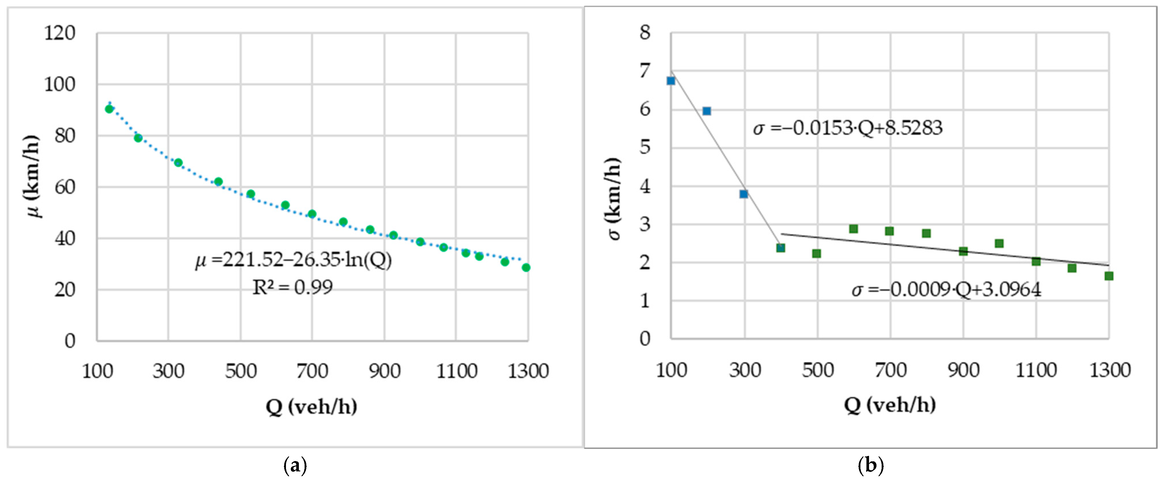For $Q\ge 136$ veh/h, the equation ${\mu }_i=221.52-26.35·\mathrm{l}\mathrm{n}\left(\mathrm{Q}\right)$ provides an excellent approximation of the Greenberg relationship (Figure 4a). For $Q<136$ veh/h, the speed is assumed to be constant at 90.5 km/h, reflecting free-flow conditions.

To define ${\sigma }_i=\sigma \left(Q\right)$, the standard deviation of vehicle speeds was analyzed concerning the flow rate, $Q$, over 5 min periods in the monitoring section. The experimental values are presented in Figure 4b. A linear regression was performed on two distinct subgroups of data points with similar trends: for $Q\ge 400$, ${\sigma }_i=-0.0009·\mathrm{Q}+3.0964$, and for $Q\le 400$, ${\sigma }_i=-0.0153·\mathrm{Q}+8.5283$. As shown in Figure 5b, these two linear equations effectively capture the trend of the standard deviation relative to the flow rate.

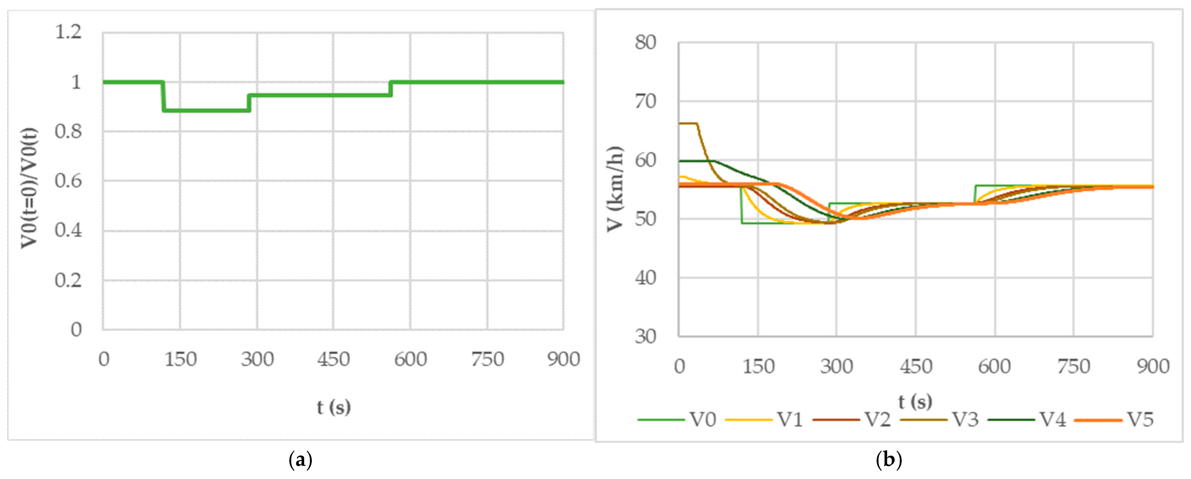
Given the homogeneity of the infrastructure downstream of the monitoring section, speed variations for the first vehicle in the simulated series $V_{i=0}\left(t\right)$ were limited. Specifically, a maximum speed reduction of 20% was allowed and over 900 s of simulation, and the average speed deviation did not exceed 5% of the initial value $V_0\left(0\right)$ (Figure 5a).

To maintain consistency with the Demand Function (DF) model used in the ISDM, the General Motors (GM) model was selected for the CFM. Given the Greenberg specification of the DF model, the CFM’s parameters were defined as $m=0$ and $l=1$, whereas for the sensitivity constant ${\alpha }_0$, the estimated value ${\alpha }_0=V_m=18.1$ km/h was used. This ensures alignment between the CFM and the ISDM, reinforcing the model’s internal consistency. Figure 5b illustrates the speed evolution of the first 5 vehicles following the lead vehicle ($i=0$) in the simulation. The CFM’s dynamics highlight the mutual conditioning between the speeds of leader–follower pairs, demonstrating the influence of the car following model on the simulated traffic stream.

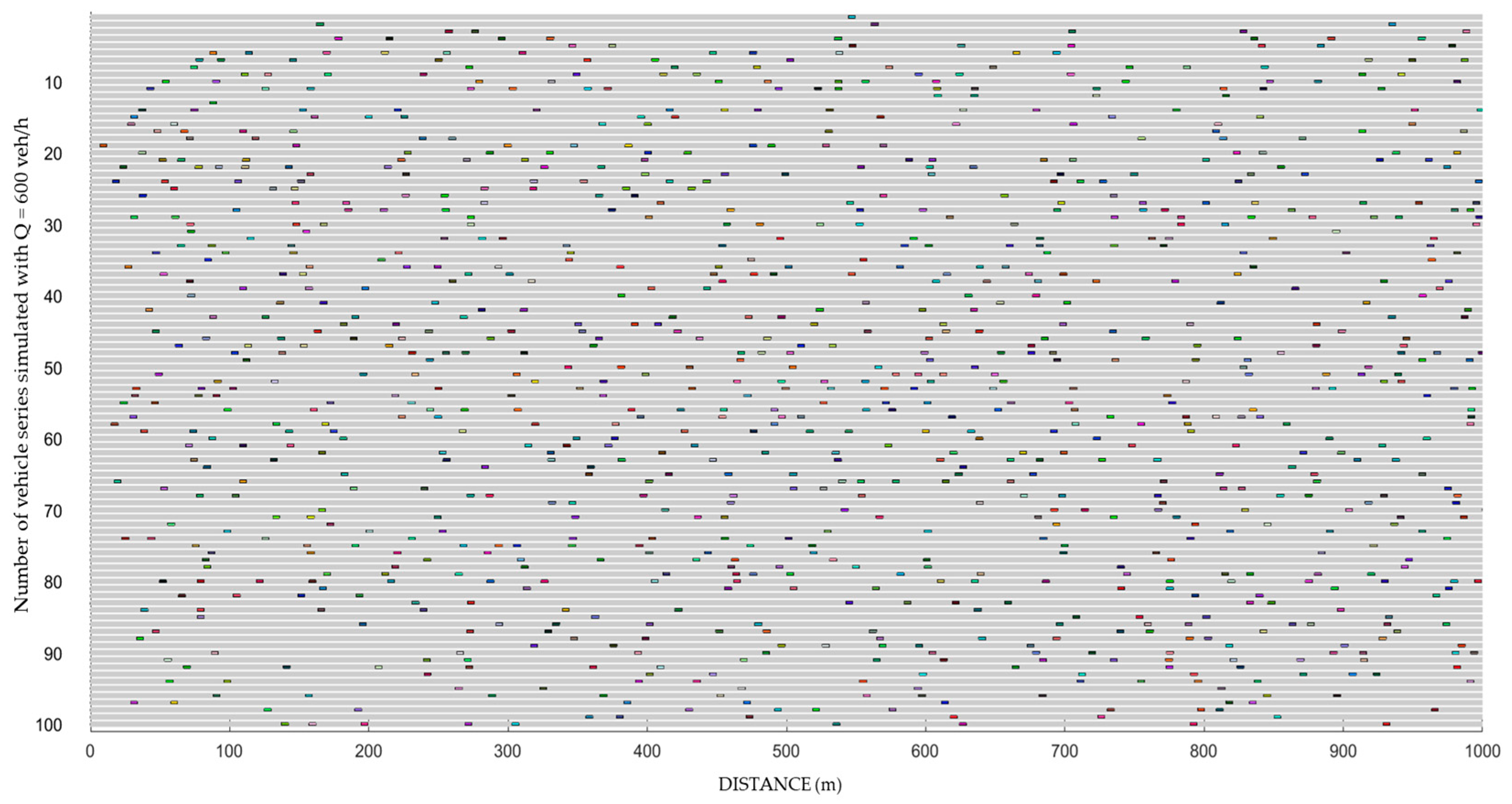
As detailed in Section 2.2, the simulation model considers hourly traffic flows between 100 veh/h and 1300 veh/h in increments of 100 veh/h. In a complete simulation session, a total of 130,000 vehicles are generated and simulated, moving along $\mathbb{r}+$ from O over an indefinite lane length. As an example, Figure 6 presents a graphical reconstruction of the results at the third simulation point, illustrating the spatial distribution of vehicles over a 1 km segment at the instant the last vehicle in the series is generated, for an average hourly traffic flow of Q = 600 veh/h.

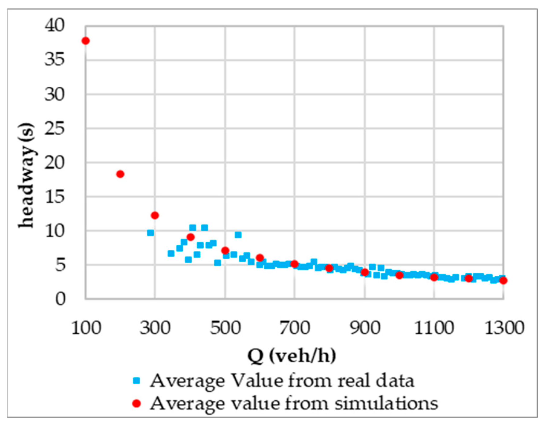
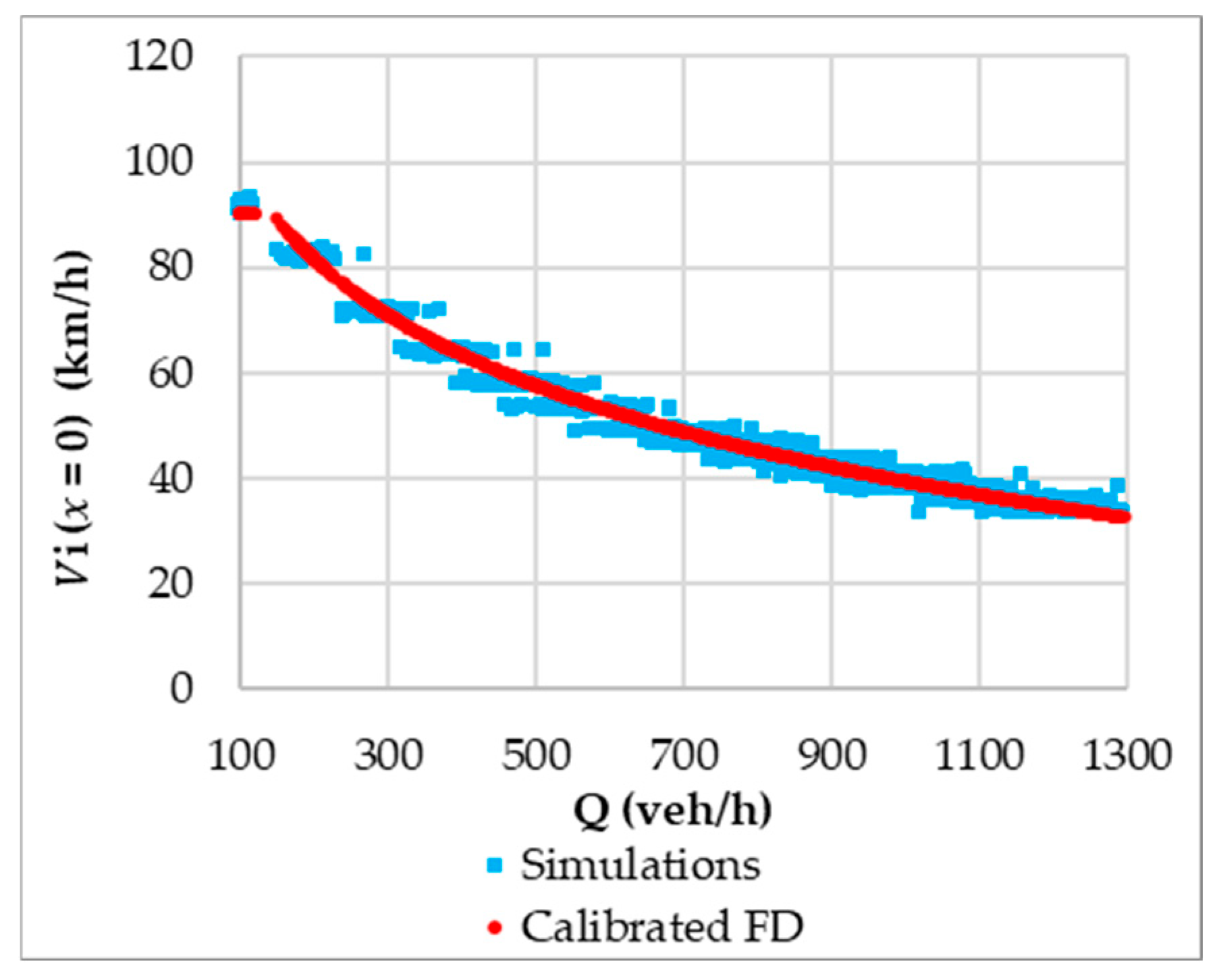
The simulated values for the temporal headways ${\tau }_{\mathrm{i}}(x=0)$ ($i=1,\dots ,100$) and the speeds $V_{\mathrm{i}}(x=0)$ ($i=1,\dots ,100$) were validated against real monitoring data. The validation results are presented in Figure 7 and Figure 8: Figure 7 demonstrates a strong agreement between the simulated temporal headway distribution and the empirical headway values observed in the monitoring section; Figure 8 confirms that the simulated entry speeds align well with the empirical speed distribution derived from the Greenberg model as a function of the hourly flow rate. These results confirm the accuracy and reliability of the simulation model in reproducing real-world traffic dynamics.

3. Results and Discussion

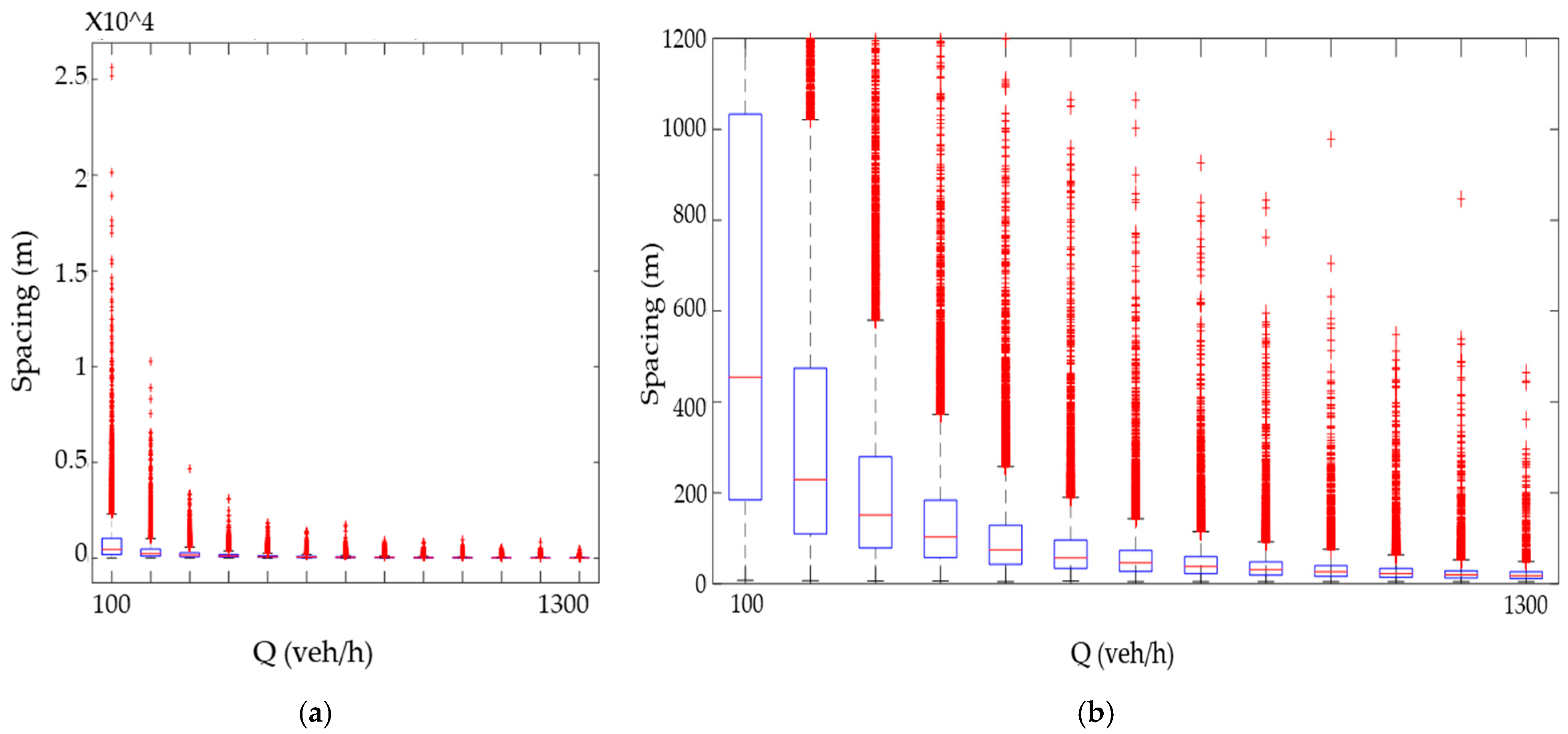
The analyzed results focus on the intervehicle spacing values $s_{\mathrm{i}}(t=t^{*})$ for $i=1,\dots ,100$ at instant $t^{*}$, corresponding to the generation of the 100th vehicle at the origin, O. To conduct this analysis, the data were classified according to the traffic flow and density levels. Specifically, the traffic flow was considered in increments of 100 vehicles per hour, ranging from 100 to 1300 veh/h, while the density values were categorized from 1 to 45 vehicles per kilometer, with increments of 1 veh/km. The simulated flow rate was calculated by normalizing the number of vehicles passing the section between $t=0$ and $t=t^{*}$ on an hourly scale. The simulated density was obtained by normalizing the total spacing of the 100 vehicles at $t=t^{*}$ over a 1 km stretch of roadway.

The statistical analysis, based on the central tendency measures and percentiles presented in

Table 1. Descriptive statistics of intervehicle spacings (m) for groupings of simulated flow rate (bins of 100 veh/h).

Q	Mean	Max	Min	50° Perc	25° Perc	75° Perc	Skewness	Kurtosis
100	922.64	25,620	6.9	454.44	184.47	1033.1	4.9943	44.637
200	403.87	10,276	6.38	229.34	109.64	474.26	4.9824	44.417
300	229.47	4677.3	5.79	150.82	78.72	279.4	4.288	35.534
400	150.6	3108.2	5.92	102.56	57.19	183.32	4.686	45.904
500	105.88	1847.2	4.57	74.225	42.585	128.61	4.6433	40.896
600	79.351	1414.5	5.63	56.705	33.38	95.99	5.4332	53.389
700	62.321	1749.1	4.53	45.64	26.7	73.255	6.9385	96.295
800	50.278	926.05	4.57	37.35	22.335	59.285	5.52	52.739
900	41.027	843.59	4.58	31.00	18.65	47.925	6.0655	63.168
1000	34.331	978.41	4.55	26.115	15.87	39.785	7.0431	91.036
1100	29.267	547.91	4.52	22.315	13.9	33.655	6.4981	63.745
1200	25.144	846.86	4.53	19.27	12.32	28.39	9.0397	133.81
1300	23.303	464.68	4.51	17.4	11.36	26.1	6.8578	72.258

, and further illustrated by the boxplot in Figure 9, revealed a progressive reduction in intervehicle spacing as the simulated flow rate increased. While the maximum spacing values experienced a significant decline, the minimum values remained relatively stable, although with a slight downward trend. This suggests that shorter vehicle gaps were largely unaffected by traffic density increases, but longer gaps became increasingly rare. Outliers observed in the boxplots are not attributed to simulation errors but are instead reflective of stochastic variability under rare, yet plausible, traffic conditions. These include transitions between free-flow and congested states or erratic spacing patterns at low-density volumes. Such behavior is consistent with natural traffic flow dynamics modeled through Monte Carlo simulation techniques. Examining the distribution of spacing values, Table 1 shows that the data consistently exhibited positive skewness, indicating a longer tail toward higher spacing values. This asymmetry reflects irregular large gaps between some vehicles. Furthermore, the analysis revealed high kurtosis, signifying a leptokurtic distribution with a sharper peak than a normal distribution. This implies a higher frequency of extreme values, both at the lower and upper ends of the spacing spectrum.

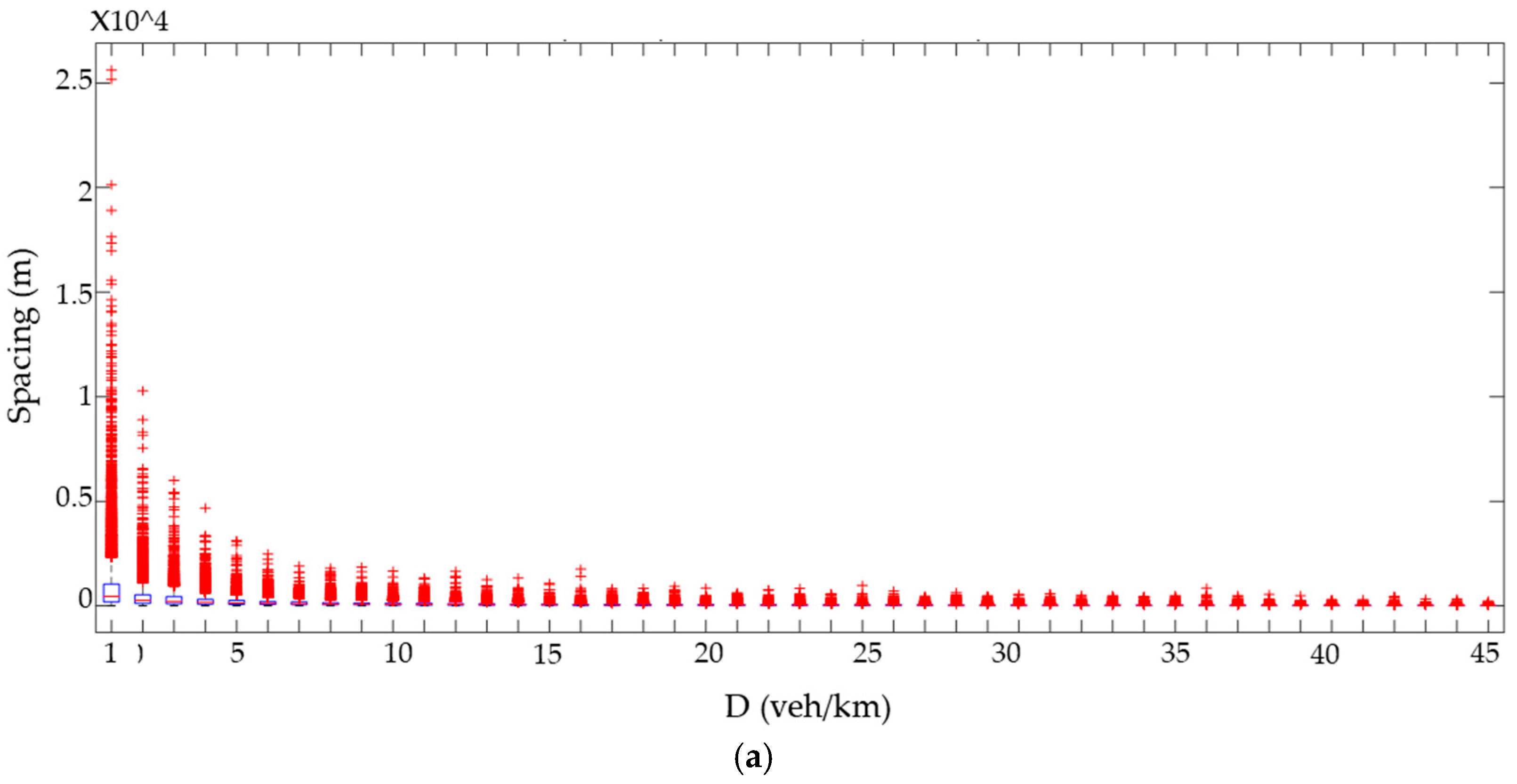
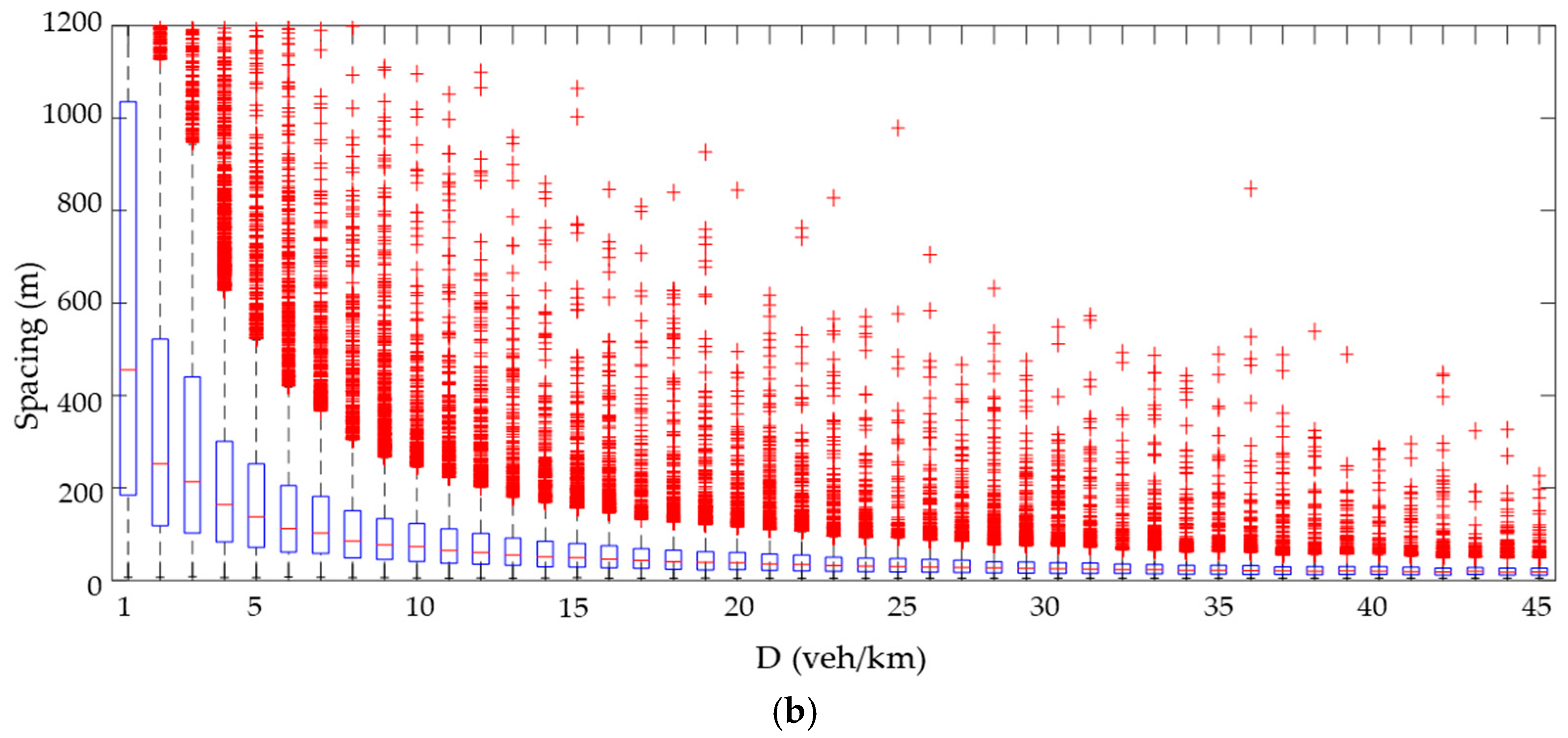
The main findings can be summarized by grouping the results into density intervals and computing the average density for each group. As shown in Figure 10 and

Table 2. Descriptive statistics of intervehicle spacings (m) for groupings of simulated density (bins of 1 veh/km).

D	Mean	Max	Min	50° Perc	25° Perc	75° Perc	Skewness	Kurtosis
1	925.25	25,620	6.90	455.05	184.57	1034.7	4.9866	44.506
2	452.7	10,276	6.38	251.81	118.3	521.75	4.9722	42.338
3	363.64	5996.2	8.37	213.47	102.13	440.13	4.1316	29.932
4	247.9	4677.3	6.27	163.82	82.905	300.66	4.2043	33.939
5	206.32	3108.2	5.79	137.25	71.375	251.88	4.2485	33.373
6	166.37	2479.2	7.07	112.18	61.465	204.94	3.7555	26.575
7	145.01	1900.9	6.70	102.35	58.12	181.34	3.2632	22.361
8	123.87	1807.6	5.92	85.145	48.53	150.81	4.5000	35.454
9	111.16	1847.2	6.06	77.15	45.13	133.78	4.1848	33.509
10	100.33	1655.8	5.63	72.66	40.915	122.8	4.3202	38.079
11	90.389	1327.8	4.57	64.815	37.04	111.28	4.7562	40.389
12	84.35	1650.9	5.48	60.72	34.915	101.53	5.6247	58.485
13	76.66	1246.5	4.53	55.18	32.945	91.585	4.9239	42.476
14	70.994	1328.2	5.36	50.865	29.475	84.765	5.1748	49.562
15	66.559	1064	5.77	49.17	28.99	79.86	5.0261	47.713
16	62.722	1749.1	4.71	46.22	27.295	74.805	8.2438	135.45
17	58.962	808.68	4.73	43.335	26.23	68.595	4.9513	40.033
18	55.487	838.67	4.57	40.685	24.02	65.065	5.0098	40.098
19	52.755	926.05	5.03	39.225	22.83	61.94	5.8383	56.421
20	50.418	843.59	4.7	38.665	23.475	60.595	4.6922	44.698
21	47.802	616.64	4.6	35.66	21.83	56.76	4.69	36.329
22	45.396	761.9	4.58	34.18	20.625	54.63	5.5251	57.891
23	43.454	827.1	4.59	32.31	19.56	49.79	6.1244	62.152
24	41.623	570.14	4.7	31.17	18.82	47.955	5.412	47.531
25	39.896	978.41	4.79	30.39	18.13	47.615	8.9377	132.33
26	38.334	704.63	4.58	29.045	17.965	45.46	6.3722	69.874
27	37.151	465.9	4.55	28.215	17.135	44.075	4.6074	35.843
28	35.781	631.47	4.58	27.07	16.31	40.525	6.1235	58.61
29	34.555	474.29	4.64	26.045	15.95	39.61	5.219	42.859
30	33.302	547.91	4.62	25.255	15.17	38.63	5.4787	49.967
31	32.19	572.09	4.57	24.79	14.845	37.715	6.6762	70.712
32	31.235	492.66	4.6	23.49	15.025	35.455	6.3429	60.215
33	30.208	487.08	4.52	23.05	14.03	34.425	6.424	62.073
34	29.476	442.7	4.57	21.615	13.48	32.665	6.175	54.662
35	28.601	489	4.62	21.7	13.64	33.03	6.454	65.582
36	27.742	846.86	4.58	20.905	12.84	31.93	11.013	190.88
37	26.987	488.07	4.59	20.425	12.94	29.745	6.7343	67.647
38	26.419	538.31	4.56	19.97	12.435	30.215	7.1225	77.327
39	25.602	488.66	4.55	20.295	12.77	30.455	6.7337	84.27
40	25.011	285.87	4.73	19.895	12.775	30.025	5.6616	48.619
41	24.427	295.18	4.6	18.905	12.175	28.525	5.0497	40.16
42	23.823	446.53	4.56	18.165	11.85	26.735	7.7868	87.562
43	23.289	323.57	4.65	19.595	12.58	27.77	6.5581	77.39
44	22.7	326.22	4.53	18.005	11.76	26.565	5.6649	57.481
45	22.006	226.68	4.56	18.165	11.73	26.625	4.3475	35.997

, both the central tendency and dispersion measures decreased as the vehicle density increased, consistent with theoretical expectations for traffic flow behavior. The distribution of the simulated data exhibited a positively skewed pattern with leptokurtic characteristics, indicating an asymmetric shape with a pronounced peak.

Assessing autocorrelation is essential for understanding the dependency between vehicle distances within each simulated vehicle sequence. In this context, the analysis focuses specifically on autocorrelation at lag1, based on the assumption that no significant correlations at higher lags should exist unless a lag1 correlation (i.e., among three consecutive vehicles) is already present. For each sequence of 100 simulated vehicles, the correlation between consecutive spacings (lag 1) was calculated. These values were extracted from both the correlation matrix and the p-value matrix. The p-value was then used to determine the statistical significance of the correlation, using the commonly accepted threshold of 0.05.

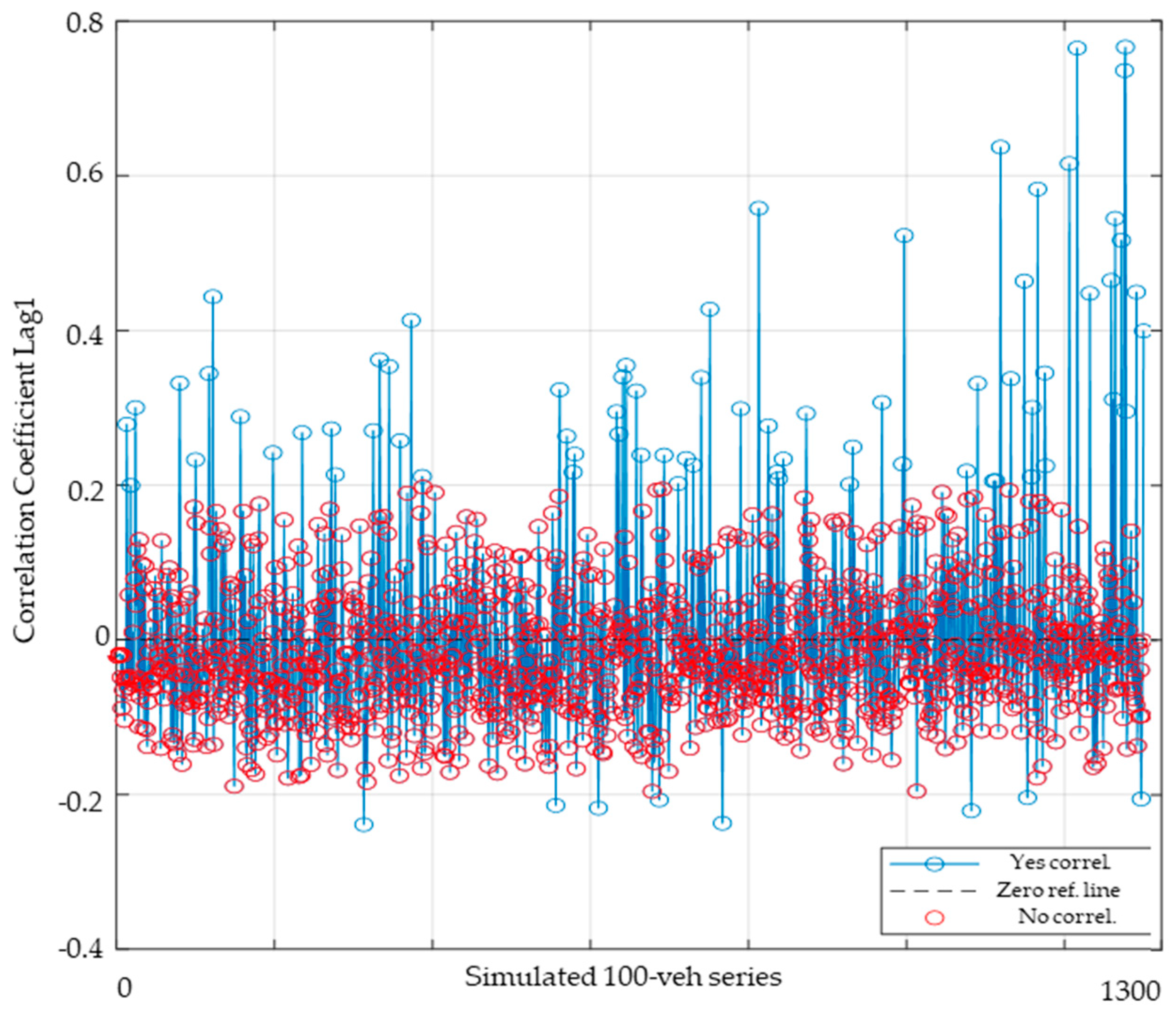
Figure 11 presents the correlation coefficient at lag 1 for each simulated vehicle sequence. Sequences where the correlation was not statistically significant (i.e., p-value > 0.05) are highlighted in red, accounting for 94% of the 1300 simulated series. According to [51], a correlation is considered weak if its absolute value falls between 0.1 and 0.3, moderate if it ranges from 0.3 to 0.5, and strong if it exceeds 0.5. Applying this classification to the 1300 simulated series, the results indicate that 73% exhibited no correlation, 24% showed a weak correlation, and only 3% displayed a moderate or strong correlation. This confirms that significant dependencies between consecutive vehicle spacings are relatively rare under the simulated traffic conditions. Figure 11 further illustrates how the autocorrelation increases with traffic volume and density. In particular, the correlation values at lag1 are generally higher in sequences simulated under higher traffic conditions. The significant autocorrelation observed in intervehicle spacing at higher traffic densities, illustrated in Figure 11, indicates the presence of short-range dependencies between consecutive vehicles. This pattern typically arises from platoon formation, where vehicles cluster due to constrained car following behavior. From a practical perspective, this autocorrelation results from drivers continuously adjusting their speed and spacing based on the actions of the vehicle immediately ahead.

In classical car following models, such as the General Motors model, this phenomenon is governed by driver characteristics, including the reaction time and the sensitivity to spacing. At higher densities, shorter distances between vehicles substantially reduce the time available for drivers to perceive and respond to the speed variations of the vehicle in front. Consequently, even minor changes in speed propagate rapidly through the vehicle platoon, magnifying the effects of each driver’s reaction delay [44,52]. As a result, small initial disturbances can quickly amplify, leading to traffic instability and pronounced fluctuations in vehicle spacing [53,54].

This interaction between delayed driver reactions and their sensitivity to spacing variations leads to the formation of stable vehicle groups—or platoons—characterized by strong temporal correlations. Within these platoons, each vehicle’s motion is directly influenced by the preceding vehicles, creating a persistent autocorrelation in spacing [55,56]. To further support the connection between autocorrelation and platooning behavior, future developments of the proposed model should incorporate more comprehensive metrics, such as the average platoon length, the vehicle membership consistency over time, and stability indices. These additional indicators would allow for a deeper understanding of the structure and persistence of vehicle groupings, offering a more detailed assessment of how traffic density and flow conditions influence platoon dynamics and the resulting impacts on road safety and operational efficiency.

Therefore, the observed autocorrelation in intervehicle spacing distributions demonstrates the inherent “memory effect” resulting from drivers’ finite reaction times and limited responsiveness. This effect contradicts the assumptions behind traditional statistical models (such as exponential or Erlang distributions), which rely on the assumption of independent, memoryless events. These findings support the need for spacing models that are not based on memoryless or independent-event assumptions, particularly in congested regimes where the driver behavior introduces dynamic memory effects.

In summary, the data analysis yielded the following key observations:

• Positive skewness: The intervehicle spacings exhibit positive skewness, indicating an asymmetric shape with a longer tail towards higher values. Most spacings cluster at lower values, but occasional, large gaps occur.
• High kurtosis: The distribution shows high kurtosis, indicating a leptokurtic shape that is more peaked than a normal distribution. This implies a higher frequency of extreme values, both low and high, compared to a normal distribution.
• Non-zero minimum value: the minimum values in the distribution are non-zero, reflecting the physical constraint that vehicle spacings cannot fall below a certain threshold.
• Autocorrelation: there is some evidence of autocorrelation at a higher traffic volume and density, where consecutive vehicle spacings show a stronger dependency due to platooning effects.

Given these statistical properties, the Pearson type III (PTIII) distribution, previously used to model vehicle headways in the THDM sub model, proved to be a highly adaptable fit for modeling intervehicle spacing. Its flexibility in capturing high asymmetry and kurtosis makes it well-suited for these conditions. The PTIII distribution can be represented by a probability density function (PDF) that depends on three parameters—$k$, $\lambda$, $s_0$—and is expressed in terms of vehicle spatial distance $s$ as follows:

$$f\left(s\right)={\displaystyle \frac{\lambda }{\mathrm{\Gamma }\left(k\right)}}·{\left[\lambda \left(s-s_0\right)\right]}^{k-1}exp\left\{-\lambda \left(s-s_0\right)\right\}\hspace{1em}for s\ge s_0$$

(10)

where $\Gamma \left(k\right)$ is the Eulerian Gamma function, which is defined as follows:

$$\Gamma \left(k\right)=\underset{0}{\overset{\mathrm{\infty }}{\int }}{x}^{k-1}exp\left\{x\right\}dx$$

(11)

This Pearson type III (PTIII) distribution is particularly suited for modeling right-skewed data, with its degree of skewness controlled by the shape parameter, k, which is restricted to positive real values. The location parameter, $s_0$ ∈ $\mathbb{R}$, shifts the distribution, $f\left(s\right)$, along the s-axis, while the scale parameter, $\lambda$, affects the spread of the distribution. In general, $\lambda$ ∈ $\mathbb{R}$ with $\lambda \ne 0$. If $\lambda >0$, then $s$ ∈ ($s_0$, $+\mathrm{\infty }$), and if $\lambda <0$, then $s$ ∈ ($-\mathrm{\infty }$, $s_0$). For the vehicle spacing distribution, the Pearson type III distribution is always considered with $\lambda >0$, ensuring that spacing values remain positive, as required by physical constraints. In addition, the choice of PTIII is further supported by its theoretical advantages over alternative asymmetric distributions typically employed in traffic and reliability modeling, such as the Weibull and the Log-Normal. Unlike these alternatives, the PTIII distribution offers greater parametric stability—i.e., less sensitivity to sampling variability and outliers—and enhanced statistical interpretability, as its parameters are directly related to key descriptive moments of the data (mean, variance, skewness). Moreover, while other distributions, such as the exponential or Erlang, require assumptions of independence and a memoryless structure, the PTIII does not impose such constraints, making it more suitable for modeling spacing data that may exhibit serial dependence. Thus, it can be adapted to model data with interdependencies, such as those revealed in the lag 1 autocorrelation analysis previously discussed and illustrated in Figure 11.

4. Conclusions

This study highlights the critical role of intervehicle spacing in traffic analysis on two-lane roads, addressing a gap in the existing literature, where temporal headways have traditionally received more attention. The findings have important implications for the development of traffic models that enhance both safety and sustainability. While modern image processing and traffic monitoring technologies have advanced significantly, their deployment remains largely restricted to sensor-rich infrastructures, such as motorways and toll roads. The high cost of sensor networks renders them impractical for widespread use on two-lane rural roads. Given the strategic importance of two-lane roads in connecting urban and interurban networks to higher-level infrastructures, this study proposed an alternative methodology to analyze spacing behavior. A simulation-based model was developed to estimate the probability density of intervehicle spacing under various traffic conditions. This model integrates macroscopic and microscopic traffic flow theories and was calibrated and validated using data from a monitoring section in Northern Italy. The simulation results generated realistic spacing distributions across a wide range of flow and density levels.

The statistical analysis of the simulated data led to several key observations:

• Positive skewness: The spacing distribution is positively skewed, indicating a longer tail toward larger values. While most vehicle spacings are clustered at the lower end, occasionally larger spacings occur.
• High kurtosis: The distribution shows high kurtosis, characterizing a leptokurtic shape that is more peaked than a normal distribution. This suggests a higher frequency of extreme values (both low and high) compared to a Gaussian model.
• Non-zero minimum value: the minimum observed spacing values remain above zero, reflecting the physical constraint that vehicles cannot be spaced below a certain safety threshold.
• Autocorrelation: at higher traffic volumes and densities, there is some evidence of autocorrelation, suggesting that spacing patterns become more structured, likely due to platooning effects.

Based on these findings, the Pearson type III (PTIII) distribution was identified as the most appropriate probability model to represent the simulated spacing data. Its flexibility makes it particularly suitable for accurately describing asymmetric distributions with high kurtosis (leptokurtic distributions). Compared to other asymmetric distributions commonly used, such as Weibull or Log-Normal, the PTIII distribution is less sensitive to sampling variability and outliers, and it offers clearer statistical interpretability. Additionally, unlike distributions commonly adopted in vehicle spacing analyses—such as the exponential or Erlang distributions—the PTIII does not require assumptions of independence or memoryless behavior, making it especially valuable for modeling realistic vehicle spacing under different traffic conditions.

It is important to highlight that this study examines only a simplified scenario, involving one-directional traffic with a low vehicle flow, no overtaking maneuvers, and a single type of vehicle, under normal conditions without severe weather or emergency events. Furthermore, this study does not include experimental spacing data from real traffic, limiting the validation of our simulation results. These simplifications were necessary to create a controlled baseline for analysis. Future work will address these limitations by incorporating empirical data and expanding the model to more realistic and complex traffic scenarios, thereby enhancing its generalizability and practical relevance. In addition to its technical contributions, this research also supports broader sustainable development goals by promoting methods for improving traffic flow efficiency, reducing congestion-related emissions, and enhancing road safety—especially in rural areas underserved by traditional traffic monitoring systems. In practical terms, the simulation model can serve as a valuable decision-supporting tool in traffic management applications, such as the optimization of dynamic speed limit systems, adaptive signal control, or congestion mitigation strategies. Moreover, its modular structure lends itself to future adaptation for mixed traffic scenarios, including those involving different levels of autonomous and connected vehicles. Evaluating its performance under these evolving conditions would be crucial to assess its scalability and relevance in next-generation transportation systems. By enabling the analysis of traffic behavior without reliance on costly infrastructure, the proposed simulation approach offers a practical tool for transportation planning in regions where investments in ITS technologies may be economically or logistically infeasible. More efficient spacing leads to smoother traffic flows, reduced fuel consumption, and fewer stop-and-go conditions—factors that directly contribute to environmental sustainability and public health.

To further develop the findings of this study, future research should focus on

• Parameter estimation for Pearson type III: Based on qualitative evidence from simulation results and characteristics of spatial headway data, the Pearson type III distribution has been identified as suitable for representing continuous distributions. Future research will focus on refining the parameters of the Pearson type III distribution to improve the statistical representation of vehicle spacings under varying arrival flow rates and density levels. This process will include formal parametric and non-parametric goodness-of-fit tests and comparative analyses.
• Traffic safety assessment: An assessment using the estimated spacing distributions to quantify the collision risk, particularly by analyzing the percentage of vehicles traveling at intervehicle distances below a critical safety threshold. This can be linked to stopping distances under real-time traffic conditions.
• Extension to other road types and traffic environments: calibrating and validating, also using experimental spacing data directly collected from real traffic situations, the simulation framework to urban road networks, multilane highways, and various traffic compositions to assess how spacing behaviors change under different conditions.
• Effects of Intelligent Transportation System (ITS) technologies: Investigating how the probabilistic model of spatial headways could be affected by ITS components under different traffic scenarios in terms of vehicle volumes and density. The specific technologies considered include Variable Speed Limit (VSL) systems, Vehicle-to-Everything (V2X) communications, and mixed traffic flows consisting of Human-Driven and Connected Autonomous Vehicles with varying levels of market penetration. This approach aims to evaluate the potential impacts of ITS integration on traffic management efficiency, flow stability, and overall road safety.

The methodology presented in this study offers a scalable, cost-effective approach for analyzing intervehicle spacing in environments where traditional sensor networks are unavailable. Its application across varied traffic contexts can significantly contribute to designing safer, more efficient, and more sustainable transportation systems, aligning with global efforts to develop equitable, eco-friendly, and resilient infrastructure.