Real-Time Modeling of a Solar-Driven Power Plant with Green Hydrogen, Electricity, and Fresh Water Production: Techno-Economics and Optimization

Abstract

Solar energy is important for the future as it provides a clean, renewable source of electricity that can help combat climate change by reducing reliance on fossil fuels via implementing various solar-based energy systems. In this study, a unique configuration for a parabolic-trough-based solar system is presented that allows energy storage for periods of time with insufficient solar radiation. This model, based on extensive analysis in MATLAB utilizing real-time weather data, demonstrates promising results with strong practical applicability. An organic Rankine cycle with a regenerative configuration is applied to produce electricity, which is further utilized for hydrogen generation. A proton exchange membrane electrolysis (PEME) unit converts electricity to hydrogen, a clean and versatile energy carrier since the electricity is solar based. To harness the maximum value from this system, additional energy during peak times is used to produce clean water utilizing a reverse osmosis (RO) desalination unit. The system’s performance is examined by conducting a case study for the city of Antalya, Turkey, to attest to the unit’s credibility and performance. This system is also optimized via the Grey Wolf multi-objective algorithm from energy, exergy, and techno-economic perspectives. For the optimization scenario performed, the energy and exergy efficiencies of the system and the levelized cost of products are found to be approximately 26.5%, 28.5%, and 0.106 $/kWh, respectively.

1. Introduction

Environmental problems such as climate change, air pollution, and water scarcity are among the most pressing global challenges, driven in large part by reliance on fossil fuels and unsustainable resources [1]. Renewable energy sources, especially solar energy, offer transformative means to address these issues. Solar energy is abundant and clean, powering technologies like concentrated solar power plants that reduce greenhouse gas emissions [2,3]. Within an intermediate temperature range, parabolic trough solar collectors (PTSCs) are the most suitable type of concentrating solar collectors for capturing solar thermal energy [4]. Furthermore, solar-driven electrolysis is integral to producing green hydrogen, a versatile energy carrier with applications in transportation, energy storage, and industry. Regarding sustainability and environmental impact, PEM water electrolysis is a preferred technology for converting renewable energy to high-purity hydrogen. This technology possesses significant advantages including a compact design, minimal footprint, elevated current density, high efficiency, functionality at moderate temperatures (20–80 °C), and the generation of high-purity hydrogen along with oxygen as a byproduct [5].

These systems also support water production through innovative desalination and purification processes, which are important for arid regions facing water shortages. Reverse osmosis (RO) is a prevalent membrane technology utilized for water desalination and purification, providing an energy-efficient method for generating fresh water from salt water or contaminated sources [6]. It operates by applying a pressure above the osmotic level to drive water through a semi-permeable membrane, effectively removing impurities, salts, viruses, and bacteria. Recent improvements have concentrated on enhancing membrane materials, system efficiency, and sustainability [6,7].

Despite challenges like high production costs, energy intermittency, and infrastructure demands, advancements in solar energy technologies and integration with hydrogen and fresh water production systems present a scalable path toward sustainability [8,9].

1.1. Background

Numerous studies on solar-driven power plants for hydrogen, electricity, and fresh water have been reported, as have investigations into the modeling, analysis, and optimization of them. For instance, with a solid-oxide fuel cell connected to a parabolic trough photovoltaic thermal collector and thermal energy storage, as well as a solar-powered proton exchange membrane electrolysis cell, Zheng et al. [10] presented a novel multigeneration system. The findings show that the parabolic trough photovoltaic thermal collector can achieve an 80.7% energy efficiency and a 33.8% exergy efficiency. The simple payback period, dynamic payback period, and net present value are 9.11 years, 11.6 years, and USD 45.8 million, respectively.

To effectively utilize solar energy, Zheng et al. [11] suggest a unique partially covered parabolic trough photovoltaic thermal (PCPTPVT) collector. According to the findings, 61.4% of the solar energy received by the PCPTPVT is converted to thermal energy for fluid heating, and 12.4% of that is converted to solar electricity. When the solar irradiation is increased from 300 W/m² to 1100 W/m², the PCPTVPT’s electrical and energy efficiencies can reach 27.9% and 64.3%, respectively.

A system comprising a proton exchange membrane electrolysis system, organic Rankine cycle, lithium bromide absorption refrigeration cycle, and parabolic trough solar collector was designed by Bedakhanian et al. [12]. The study’s objective functions were cost rate and energy efficiency. The optimal energy efficiency rate was found to be 3.12%, while the system cost rate was USD 16.4 per hour. Under ideal circumstances, the system can generate 15.4 kW of power, 0.189 kg of hydrogen per day, and 56.2 kW of cooling.

A medium-to-high-temperature solar-integrated energy system was proposed by Zhang et al. [13]. The system is comprised of four subsystems: electrodialysis, multi-effect distillation (MED), an organic Rankine cycle (ORC), and a parabolic trough collector (PTC). When the direct normal irradiance is 500 W/m², the system is found to produce 107 kg/h of desalinated water, 10.6 kg/h of NaOH, and 48.5 kg/h of HCl.

Maya et al. [14] investigated the key factors affecting the performance of a proton-exchange-membrane-type electrolyzer as well as the risk of explosion under various operating situations, particularly when the electrolyzer is working at high pressure and with a changeable solar energy power source. The primary conclusions of this work are that an electrolyzer cannot operate safely all day long for a solar energy supply running at high pressure because low current densities favor large hydrogen concentrations at the anode during hours when solar irradiation is low.

In order to generate power and lessen power production variations in renewable energy technologies, proton exchange membrane fuel cells (PEMFCs) and proton exchange membrane electrolyzer cells (PEMECs) can be combined. Abdollahipour et al. [15] have examined this by numerically simulating a three-dimensional model of a PEMFC and PEMEC. The efficiency and output power of the power generation system were found to be 0.323 and 1800 W m⁻², respectively.

Astrani et al. [16] optimized RE parks for three scenarios: photovoltaic (PV) only, hybrid PV–wind, and wind only. The goal was to produce green hydrogen in areas with varying potentials for renewable energy. An electrolyzer with a proton exchange membrane (PEM) is used to permit quick reactions to RE variations. Wind-only designs have the lowest LCOH, at 4.26 $/kg H₂, while PV-only configurations yield the highest LCOH, at 14.4 $/kg H₂.

Abedi et al. [17] proposed a system integrating a solar chimney with a humidification–dehumidification desalination process, utilizing solar energy to generate buoyant air for desalination without additional energy input. The model indicates that a large-scale solar desalination chimney could provide fresh water for over 800 households, while smaller systems could produce approximately 600 L per day for individual homes. This approach aligns with the present study’s focus on solar-powered desalination, emphasizing energy efficiency and scalability.

Kianfard et al. [18] conducted energy and exergoeconomic analyses for a novel system that produces hydrogen and distilled water. This cogeneration system combines a reverse osmosis (RO) desalination unit, a proton exchange membrane (PEM) electrolyzer, and a geothermal-driven dual-fluid organic Rankine cycle (ORC). The product hydrogen costs were 4.26 $/kg, whereas the distilled water costs were 0.333 $/m³ based on the exergoeconomic analysis and a unit exergy cost of 1.3 $/GJ for geothermal hot water.

1.2. Rationale for Study

The rising global need for sustainable energy options highlights the need for integrated systems that can efficiently generate electricity, hydrogen, and clean water. Although individual technologies such as parabolic trough solar collectors (PTSCs), sensible thermal storages, proton exchange membrane electrolyzers (PEMEs), and reverse osmosis (RO) units have been extensively examined, the incorporation of real-time weather data and meteorological conditions to evaluate the economic and energy performance of the integrated system considered here is still insufficiently investigated. This study fills this gap by proposing a multigeneration design that integrates all technologies into a singular optimal framework in a theoretical context, and lays the groundwork for future work that can explore practical aspects.

To address the complexity and real-world viability of the proposed multigeneration system, the present study seeks to answer the following research questions:

• How does the performance of the thermal storage tank vary across different months of the year, and how does this influence the overall system performance?
• How do seasonal variations affect the rates of electricity, hydrogen, and fresh water production?
• Which components of the system contribute most to exergy destruction, and how can this information guide future improvements?
• How do changes in key parameters—such as solar radiation intensity, turbine inlet temperature, and electricity allocation strategy—affect system efficiencies and product outputs?
• What are the trade-offs between cost and efficiency in the system, and how can multi-objective optimization help identify the best balance?

This study’s key objectives and contributions are outlined as follows:

• Proposing an integrated energy system that utilizes solar energy and thermal storage to ensure uninterrupted generation of electricity, hydrogen, and clean water, even in the absence of sunlight.
• Examining the impact of electricity allocation strategies on system efficiency and economic feasibility by studying scenarios in which electricity is allocated for hydrogen production, fresh water generation, or direct grid sales.
• Performing extensive thermodynamic and economic evaluations via parametric studies and multi-objective optimization to determine the trade-offs between efficiency and cost.
• Conducting a real-time case study in Antalya, Turkey, to analyze system performance hourly over the course of a year, thereby offering insights into its practical application under actual operational settings.
• Employing multi-objective optimization methods to address energy, exergy, and economic factors, for achieving an ideal balance between efficiency and cost.

This study enhances sustainable energy technology and offers a practical framework for optimizing renewable energy use in multigeneration systems.

2. System Description

A schematic diagram of the proposed system is depicted in Figure 1. The system consists of four subsystems: a parabolic trough solar collector with a sensible thermal storage tank, an organic Rankine cycle, a reverse osmosis desalination unit, and a proton exchange membrane electrolyzer. In the ORC, thermal energy from the solar and storage components is absorbed in the evaporator, where the leaving working fluid (3) enters the turbine to generate electricity that will be transmitted to the grid, the PEME unit, and the reverse osmosis cycle. The expanded fluid at the turbine exit (4) has a comparatively elevated temperature and is used to preheat the evaporator inlet (5) via a recuperator. The recuperator’s outlet (6) subsequently feeds into the condenser to transfer heat to the cooling water. The working fluid next enters a pump (1), where its pressure is elevated, and then proceeds to the recuperator (2), where its temperature is raised.

Seawater enters the reverse osmosis system at point 7. The feed pump increases the seawater pressure, after which the fluid enters the high-pressure pump (HPP) at state 8, where it is pressurized to beyond the osmotic pressure necessary for desalination. The pressurized seawater subsequently enters the initial reverse osmosis module (RO-1) at state 9, where it undergoes partial desalination. In RO-1, the water is divided into two streams: permeate (purified water), which exits at point 10, and concentrate (brine), which exits at point 11.

The brine from RO-1 then flows to the booster pump (BP), which elevates its pressure and directs it to the second reverse osmosis module (RO-2) at state 12. In RO-2, the brine undergoes further desalination, producing more permeate that exits at point 13, and merges with the permeate from RO-1 at point 15. The residual concentrated brine departs from RO-2 at point 14 and proceeds to the Pelton turbine, where energy is extracted from the high-pressure brine prior to it being discarded as waste.

In the proton exchange membrane electrolyzer (PEME) system, water enters the heat exchanger at ambient temperature (b1) and is subsequently heated to 80 °C, preparing it for entering the PEM electrolyzer. The heat exchanger enables optimal temperature control by utilizing solar energy to support the PEME process.

Water at the electrolyzer temperature flows to the PEM electrolyzer, where it undergoes electrolysis. Electrolysis produces hydrogen and a combination of oxygen and water. The generated hydrogen is subsequently cooled and stored in a tank. The mixture of oxygen and water from the electrolyzer flows to an Oxygen Separation unit, where oxygen is separated from the water and then stored. Simultaneously, the heated water re-enters the PEM electrolyzer, establishing a recirculation loop.

The solar and storage elements of the system function in two modes, charging and discharging, depending upon the availability of solar energy. During the charging mode, Therminol VP-1, the heat transfer fluid of the solar and storage units, circulates through the solar field, absorbing heat produced by the parabolic trough collectors at state 17. The heated fluid then exits the solar collectors (18) and is divided into two separate streams. One stream passes through the heat exchanger, transferring heat to the ORC and PEME (19), and the other delivering heat to the thermal tank for storage, to be utilized later in discharging mode (21). The fluid leaving the heat exchanger at state 20 merges with the stream from the thermal storage tank (22) before entering the pump at state 23. During the discharging mode, the thermal energy stored in the tank is used to power the ORC. The fluid exits the thermal tank at state 24, flows through the heat exchanger to transfer energy to the ORC and the PEME, and subsequently returns to the tank at state 25′.

Assumptions and Input Data

This study employs the following assumptions to simplify the modeling and analysis process:

-

The proposed system is presumed to function at steady-state conditions [4].

-

All turbomachinery is presumed to operate as adiabatic devices [19].

-

Pressure losses are assumed to be negligible throughout the system [19].

-

Heat exchange with the environment is disregarded for all system components, except for the solar collector and thermal storage tank, owing to its minimal impact [4].

-

Variations in kinetic and potential energy are considered negligible and hence are disregarded [19].

Input data for the simulation of the multigeneration plant are presented in

Table 1. Input data for the multigeneration plant simulation.

Parameter	Unit	Value	Ref.
Reference pressure, $P_0$	$\mathrm{a}\mathrm{t}\mathrm{m}$	$1$
Reference temperature, $T_0$	$\mathrm{K}$	$298.15$
Solar unit
Collector width, $w$	$\mathrm{m}$	$5.76$	[20]
Collector length, $L$	$\mathrm{m}$	$7.8$	[21]
Focal length, $F$	$\mathrm{m}$	$1.84$	[21]
Receiver efficiency, ${\eta }_r$		$0.765$	[20]
Beam solar irradiance (during times of low availability), $G_b$	$\mathrm{k}\mathrm{W}/{\mathrm{m}}^2$	$0.5$	[20]
Beam solar irradiance (during times of high availability), $G_b$	$\mathrm{k}\mathrm{W}/{\mathrm{m}}^2$	$0.85$	[20]
Emittance of receiver cover,${ϵ}_r$		$0.92$	[20]
Total number of collectors per single row,${Col}_n$		$50$
Total number of solar collector rows,${Col}_r$		$7$
Mass of oil in the tank,${\dot{m}}_r$	$\mathrm{k}\mathrm{g}/\mathrm{s}$	$8$
Diameter,$D_{r,i}$	$\mathrm{m}$	$0.045$	[20]
Reflectance of mirror,${\rho }_c$		$0.931$	[20]
Intercept factor,$\gamma$		$0.93$	[20]
Transmittance of glass cover,$\tau$		$0.94$	[20]
Absorbance of receiver,$\alpha$		$0.94$	[20]
Incidence angle modifier,$K_{\gamma }$		$1$	[20]
Storage unit
Diameter of storage tank,$d$	$\mathrm{m}$	$9$
Height of storage tank,$h$	$\mathrm{m}$	$8$
Number of storage tanks		3
Rankine cycle
Isentropic efficiency of turbine, ${\eta }_{is,t}$	$\mathrm{\%}$	$85$	[18]
Isentropic efficiency of pump, ${\eta }_{is,p}$	$\mathrm{\%}$	$80$	[18]
PPTD of evaporator, ${PP}_{ev}$	$\mathrm{K}$	5	[18]
PPTD of recuperator, ${PP}_{rec}$	$\mathrm{K}$	15	[18]
PPTD of condenser, ${PP}_{cd}$	$\mathrm{K}$	10	[18]
PEME
Oxygen output pressure, $P_{O_2}$	$\mathrm{b}\mathrm{a}\mathrm{r}$	1
Hydrogen output pressure, $P_{H_2}$	$\mathrm{b}\mathrm{a}\mathrm{r}$	1
Operating temperature of PEME, $T_{PEM}$	°C	80	[19]
Activation energy for anode reaction, $E_{act,a}$	$\mathrm{k}\mathrm{J}/\mathrm{m}\mathrm{o}\mathrm{l}$	76	[19]
Activation energy for cathode reaction, $E_{act,c}$	$\mathrm{k}\mathrm{J}/\mathrm{m}\mathrm{o}\mathrm{l}$	18	[19]
Stoichiometric coefficient or air–fuel ratio at anode, ${\lambda }_a$		14	[19]
Stoichiometric coefficient or air–fuel ratio at cathode, ${\lambda }_c$		10	[19]
Reference current density at anode, $J_a^{ref}$	$\mathrm{A}/{\mathrm{m}}^2$	$1.7\times {10}^5$	[19]
Reference current density at cathode, $J_c^{ref}$	$\mathrm{A}/{\mathrm{m}}^2$	$4.6\times {10}^3$	[19]
Reverse osmosis unit
Isentropic efficiency of pumps, ${\eta }_{is,FP}, {\eta }_{is,HPP}, {\eta }_{is,BP}$	$\mathrm{\%}$	76.7	[22]
Isentropic efficiency of Pelton turbine, ${\eta }_{is,Pelton}$	$\mathrm{\%}$	79	[22]
Water inlet temperature of RO unit, $T_7$	$\mathrm{K}$	298	[22]
Desalination rate of RO-1		0.55	[22]
Desalination rate of RO-2		0.6	[22]

. The data consist of values assumed by the authors and those sourced from established references. While the system configuration is original, reference data are used for commonly accepted parameters and constants to ensure consistency and support the assumptions made for certain values.

3. System Modeling and Analysis

3.1. Thermodynamic Analysis

In the thermodynamic modeling of the current system, each component in the various cycles is regarded as a control volume. The corresponding mass and energy balance equations for steady-state conditions are applied as follows:

$$\sum _{in}\dot{m}=\sum _{out}\dot{m}$$

(1)

$$\dot{Q}+\sum _{in}\dot{m}h=\sum _{out}\dot{m}h+\dot{W}$$

(2)

3.1.1. RO Unit

The corresponding mass rate balance equations of the reverse osmosis unit are presented below [23]:

$${\left(\dot{m}{y}_s\right)}_9={\left(\dot{m}y\right)}_{10}+{\left(\dot{m}{y}_s\right)}_{11}$$

(3)

$${\left(\dot{m}{y}_s\right)}_{12}={\left(\dot{m}y\right)}_{13}+{\left(\dot{m}{y}_s\right)}_{14}$$

(4)

$${\left(\dot{m}y\right)}_{10}={\left(\dot{m}y\right)}_{13}+{\left(\dot{m}y\right)}_{15}$$

(5)

The energy and exergy balance rate equations of the components of the RO unit are shown in Appendix A in

Table A1. Mass, energy, and exergy balances of system components.

Component	Energy Rate Balances and Relations	Exergy Rate Balance
ORC
Recuperator	${\dot{Q}}_{evap}={\dot{m}}_2\left(h_5-h_2\right)={\dot{m}}_4\left(h_4-h_6\right)$	${\dot{E}}_D={{(\dot{E}}_4-{\dot{E}}_6)-(\dot{E}}_5-{\dot{E}}_2)$
ORC pump	${\dot{W}}_{Pump}={\dot{m}}_1(h_2-h_1)$	${\dot{E}}_D={\dot{W}}_{Pump}-\left({\dot{E}}_2-{\dot{E}}_1\right)$
	${\eta }_{is,Pump}=(h_1-h_{2s})/(h_1-h_2)$
Tur	${\dot{W}}_{Tur}={\dot{m}}_3(h_3-h_4)$	${\dot{E}}_D=\left({\dot{E}}_3-{\dot{E}}_4\right)-{\dot{W}}_{Tur}$
	${\eta }_{is,Tur}=(h_3-h_4)/(h_3-h_{4s})$
Cond	${\dot{Q}}_{Cond}={\dot{m}}_1\left(h_6-h_1\right)={\dot{m}}_{18}\left(h_{w2}-h_{w1}\right)$	${\dot{E}}_D=\left(h_6-h_1\right)-\left(h_{w2}-h_{w1}\right)$
Evap	${\dot{Q}}_{evap}={\dot{m}}_3\left(h_5-h_3\right)={\dot{m}}_{22}\left(h_{22}-h_{23}\right)$	${\dot{E}}_D={{(\dot{E}}_{24}-{\dot{E}}_{25})-(\dot{E}}_3-{\dot{E}}_5)$
RO unit
FP	${\dot{W}}_{FP}{=\dot{V}}_7(P_8-P_7)/{\eta }_{FP}$	${\dot{E}}_D={\dot{W}}_{FP}-\left({\dot{E}}_8-{\dot{E}}_7\right)$
HPP	${\dot{W}}_{HPP}{=\dot{V}}_8(P_9-P_8)/{\eta }_{HPP}$	${\dot{E}}_D={\dot{W}}_{HPP}-\left({\dot{E}}_9-{\dot{E}}_8\right)$
BP	${\dot{W}}_{BP}={\dot{V}}_{11}(P_{12}-P_{11})/{\eta }_{BP}$	${\dot{E}}_D={\dot{W}}_{BP}-\left({\dot{E}}_{12}-{\dot{E}}_{11}\right)$
Pelton turbine	${\dot{W}}_{PT}={\dot{m}}_{16}(h_{14}-h_{16})$	${\dot{E}}_D=\left({\dot{E}}_{14}-{\dot{E}}_{16}\right)-{\dot{W}}_{PT}$
RO1		${\dot{E}}_D={{(\dot{E}}_9)-(\dot{E}}_{10}+{\dot{E}}_{11})$
RO2		${\dot{E}}_D={{(\dot{E}}_{12})-(\dot{E}}_{13}+{\dot{E}}_{14})$
PTC and TES
Solar pump	${\dot{W}}_{Pump}={\dot{m}}_{17}(h_{17}-h_{24})$	${\dot{E}}_D={\dot{W}}_{Pump}-\left({\dot{E}}_{17}-{\dot{E}}_{24}\right)$
	${\eta }_{is,Pump}=(h_{17}-h_{24s})/(h_{17}-h_{24})$
PTC field	${\dot{Q}}_u={\dot{m}}_{17}\left(h_{18}-h_{17}\right)$	${\dot{E}}_D={\dot{E}}_{sun}+{\dot{E}}_{l,ptc}+{\dot{E}}_{17}-{\dot{E}}_{18}$
Storage tank—charge mode	${\dot{Q}}_{l,tank}={\dot{m}}_{21}\left(h_{21}-h_{22}\right)$	${\dot{E}}_D={\dot{E}}_{l,tank}+{\dot{E}}_{21}-{\dot{E}}_{22}$
Storage tank—discharge mode	${\dot{Q}}_{l,tank}={\dot{m}}_{24}\left(h_{24}-h_{25\prime }\right)$	${\dot{E}}_D={\dot{E}}_{l,tank}+{\dot{E}}_{24}-{\dot{E}}_{25\prime }$
PEME
PEME HEX	${\dot{Q}}_{hex,peme}={\dot{m}}_{in,peme}\left(h_{c1}-h_{b1}\right)={\dot{m}}_{18}\left(h_{25}-h_{25\prime }\right)$	${\dot{E}}_D={{(\dot{E}}_{25}-{\dot{E}}_{25\prime })-(\dot{E}}_{c1}-{\dot{E}}_{b1})$
PEME		${\dot{E}}_D={{(\dot{W}}_{peme}+{\dot{E}}_{c1})-(\dot{E}}_{d1}+{\dot{E}}_{e1}+{\dot{E}}_{f1})$

and

Table A2. Component, purchased equipment cost function, ref. year, and cost index [30,31,32,33,34].

Component	Purchased Equipment Cost Function	Ref. Year	Cost Index
Turbine	$Z_{tur}=4405{\left({\dot{W}}_{tur}\right)}^{0.8}$	2005	468.2
Condenser	$Z_{cond}=150{\left(A_{cond}\right)}^{0.8}$	1968	113.7
HEX	$Z_{hex}=2143{\left(A_{HEX}\right)}^{0.514}$	1986	318.4
Tank	$Z_{tank}=\mathrm{1,15}\times 10000\times {\left(0.2{ V}_{tank}\right)}^{0.53}$	2005	468.2
Solar	$Z_{solar}=150\times {\left(A_{solar}\right)}^{0.8}$	2010	550.8
ORC and solar pump	$Z_{pump}=3540\times {\left({\dot{W}}_{pump}\right)}^{0.8}$	2011	585.7
Recuperator	$Z_{recup}=1.3(310 A_{Rec}+190)$
PEME	$Z_{peme}=1000 {\dot{W}}_{peme}$
H2 storage tank	$Z_{tank,H2}=100 V_{tank,H2}$
FP	$Z_{FP}=1.471\times {996\times \left({\displaystyle \frac{\dot{V}}{24}}\right)}^{0.8}$
HPP	$Z_{HPP}=1.471\times 81{\left(\left({\displaystyle \frac{\dot{V}}{24}}\right){\displaystyle \frac{\Delta P}{1000}}\right)}^{0.96}$
BP	$Z_{BP}=1.471\times 81{\left(\left({\displaystyle \frac{\dot{V}}{24}}\right){\displaystyle \frac{\Delta P}{1000}}\right)}^{0.96}$
Pelton turbine	$Z_{PT}=1.471\times 54{\left(\left({\displaystyle \frac{\dot{V}}{24}}\right){\displaystyle \frac{\Delta P}{1000}}\right)}^{0.96}$

.

3.1.2. Proton Exchange Membrane Electrolyzer (PEME)

Energy and exergy assessments of a PEM electrolyzer can be performed concurrently with electrochemical modeling.

The mass flow rate of the generated hydrogen can be determined as follows [19]:

$${\dot{N}}_{H_2,out}={\displaystyle \frac{J}{2F}}={\dot{N}}_{H_{2}O,reacted}$$

(6)

where $J$ denotes current density, $F$ the Faraday constant, and ${\dot{N}}_{H_{2}O,reacted}$ the rate at which water (H₂O) is consumed during the process.

The performance of the proton exchange membrane electrolyzer can be assessed using the electrochemical method outlined in reference [19]:

$$Q_{electric}=E_{electric}=JV$$

(7)

$$V=V_0+V_{act,a}+V_{act,c}+V_{ohm}$$

(8)

$$V_0=1.229-8.5\times {10}^{-4}(T_{PEM}-298)$$

(9)

In this model, the reversible potential, $V_0$, is determined using the Nernst equation. The variables $V_{act,a}$, $V_{act,c}$, and $V_{ohm}$ correspond to the activation overpotential at the anode, the activation overpotential at the cathode, and the ohmic overpotential of the electrolyte, respectively.

The excess ohmic potential across the PEME arises from the membrane’s resistance to hydrogen ion transport. The ionic resistance is influenced by several factors, including the degree of membrane humidification, the membrane thickness, and its temperature. The local ionic conductivity of the membrane, denoted as σ(x), is empirically evaluated as follows [19]:

$$\sigma \left[\lambda \left(x\right)\right]=\left[0.5139\lambda \left(x\right)-0.326\right]\exp \left[1268\left({\displaystyle \frac{1}{303}}-{\displaystyle \frac{1}{T}}\right)\right]$$

(10)

Here, $x$ denotes the depth within the membrane, measured from the interface between the cathode and the membrane, while $\lambda \left(x\right)$ indicates the water content at the specified location $x$ within the membrane. The value of $\lambda \left(x\right)$ can be determined using the water content present at the membrane–electrode interfaces as follows [19]:

$$\lambda \left(x\right)={\displaystyle \frac{{\lambda }_a-{\lambda }_c}{D}}x+{\lambda }_c$$

(11)

Here, $D$ represents the membrane thickness, and ${\lambda }_a$ and ${\lambda }_c$ denote the water content at the anode–membrane and cathode–membrane interfaces, respectively. With these parameters, the total ohmic resistance of the proton exchange membrane, $R_{PEM}$, can be determined [19]:

$$R_{PEM}={\int }_0^L{\displaystyle \frac{dx}{\sigma \left[\lambda \left(x\right)\right]}}$$

(12)

The ohmic overpotential can be calculated using Ohm’s law:

$$V_{ohm}=J{R}_{PEM}$$

(13)

The activation overpotential indicates the activity level of the electrodes and signifies the extra overpotential needed to facilitate the electrochemical reaction. The activation overpotential for the electrodes can be expressed as follows [19]:

$$V_{act,i}={\displaystyle \frac{RT}{F}}{\sinh }^{-1}\left({\displaystyle \frac{J}{2J_{0,i}}}\right) , i=a,c$$

(14)

The exchange current density in the proton exchange membrane (PEM) electrolysis process can be described as follows [19]:

$$J_{0,i}={J_i}^{ref}\exp \left(-{\displaystyle \frac{E_{act,i}}{RT}}\right), i=a,c$$

(15)

Here, ${J_i}^{ref}$ denotes the pre-exponential factor, and $E_{act,i}$ the activation energy, specific to the anode and cathode, respectively.

3.1.3. PTSC

This subsection presents the energy analysis of the parabolic trough solar collector (PTSC). The useful power from the collector ${\dot{Q}}_u$ can be expressed as follows [24]:

$${\dot{Q}}_u={\dot{m}}_r\left(C_{pr,o}{T}_{r,o}-C_{pr,i}{T}_{r,i}\right)$$

(16)

The useful power and the oil mass flow rate in the receiver, denoted as ${\dot{m}}_r$, are key parameters. Here, the subscripts “$r$”, “$i$”, and “$o$”refer to the receiver, inlet, and outlet, respectively. This useful energy rate can also be expressed as follows [24]:

$${\dot{Q}}_u=A_{ap}{F}_R\left(S-A_r/A_{ap}{U}_L\left(T_{r,i}-T_0\right)\right)$$

(17)

The variables include the aperture area of the collector ($A_{ap}$), the heat removal factor ($F_R$), the radiation absorbed by the receiver ($S$), the area of the receiver ($A_r$), and the overall heat loss coefficient of the solar collector ($U_L$). The aperture area is defined as follows [24]:

$$A_{ap}=\left(w-D_{c,o}\right)L$$

(18)

The aperture area is calculated based on the collector width ($w$), the cover’s outer diameter ($D_{c,o}$), and the collector length ($L$). The radiation absorbed by the receiver can be written as follows [24]:

$$S=G_b{\eta }_r$$

(19)

The absorbed radiation by the receiver is the product of the solar radiation intensity, $G_b$, and the receiver efficiency, ${\eta }_r$. The receiver efficiency can be defined as follows [20]:

$${\eta }_r={\rho }_C\gamma \tau \alpha K_{\gamma }$$

(20)

The receiver efficiency incorporates several factors: the mirror’s reflectance (${\rho }_C$), the intercept factor ($\gamma$), the transmittance of the glass cover ($\tau$), the receiver’s absorbance ($\alpha$), and the incidence angle modifier ($K_{\gamma }$). Values for these parameters are provided in Table 1. The heat removal factor is defined as follows [20]:

$$F_R={\displaystyle \frac{{\dot{m}}_r{C}_{p_r}}{A_p{U}_L}}\left(1-\exp \left(-{\displaystyle \frac{A_r{U}_L{F}_1}{{\dot{m}}_r{C}_{p_r}}}\right)\right)$$

(21)

The heat removal factor is dependent on $C_{p_r}$, the specific heat capacity of the oil in the receiver, and $F_1$, the collector efficiency factor. The collector efficiency factor is defined as follows [20]:

$$F_1=U_o/U_L$$

(22)

The solar collector heat loss coefficient considers the convective heat transfer coefficient between the cover and the ambient, and is expressible as follows [20]:

$$U_L={\left({\displaystyle \frac{A_r}{\left(h_{c,ca}+h_{r,ca}\right)A_c}}+1/h_{r,cr}\right)}^{-1}$$

(23)

The convection heat transfer coefficient between the cover and the ambient, denoted as $h_{c,ca}$, can be written as [24]

$$h_{c,ca}=(Nu{k}_{air}/D_{c,o})$$

(24)

The convection heat transfer coefficient $h_{c,ca}$ is calculated using the Nusselt number $\left(Nu\right)$, the thermal conductivity of air ($k_{air}$), and the outer diameter of the cover ($D_{c,o}$). The radiation heat transfer coefficient is expressed as follows [24]:

$$h_{r,ca}={\epsilon }_{CV}\sigma \left(T_c+T_a\right)\left({T_c}^2+{T_a}^2\right)$$

(25)

The radiation heat transfer coefficient accounts for temperature ($T$), emittance (${\epsilon }_{CV}$), and the Stefan–Boltzmann constant ($\sigma$), with the subscripts $c$ and $a$ indicating cover and ambient, respectively. The radiation heat transfer coefficient between the cover and receiver can be written as follows [24]:

$$h_{r,cr}=\left({\displaystyle \frac{\sigma \left(T_c+T_{r,av}\right)\left({T_c}^2+{T_{r,av}}^2\right)}{1/{\epsilon }_r+A_r/A_c\left(\frac{1}{{\epsilon }_{CV}}-1\right)}}\right)$$

(26)

The overall heat transfer coefficient can be expressed as follows [24]:

$$U_o={\left({\displaystyle \frac{1}{U_L}}+{\displaystyle \frac{D_{r,0}}{h_{c,r,i}{D}_{r,i}}}+\left({\displaystyle \frac{D_{r,0}}{2K_r}}\ln \left({\displaystyle \frac{D_{r,0}}{D_{r,i}}}\right)\right) \right)}^{-1}$$

(27)

where $h_{c,r,i}$ is specified as [24]

$$h_{c,r,i}={\displaystyle \frac{{Nu}_r{K}_r}{D_{r,i}}}$$

(28)

and the subscript “$r$” denotes the receiver.

The solar radiation rate incident on the collector can be determined as follows [21]:

$${\dot{Q}}_s=A_a·G_b$$

(29)

The thermal efficiency of the PTSC can be calculated as follows [21]:

$${\eta }_{th}={\displaystyle \frac{{\dot{Q}}_u}{{\dot{Q}}_s}}$$

(30)

3.1.4. Thermal Storage Tank

This study employs a well-mixed sensible heat storage tank, which provides the heat needed for the ORC during periods of insufficient solar energy. The working fluid chosen for circulation between the solar collector and the storage tank is Therminol VP-1 oil, which functions efficiently within a temperature range of 373 K to 623 K [20], and operates at a pressure of 500 kPa. The cylindrical heat storage tank is made of steel plate with a density of 7800 kg m⁻³, a specific heat capacity of 0.46 kJ kg⁻¹ K⁻¹, and a thickness of 0.006 m [25]. Glass wool functions as the insulating material for the storage tank. It is assumed that the oil within the tank is homogeneous, permitting the simplification that the storage tank temperature, $T_{st}$, is constant throughout the tank and varies solely with time [25].

The energy rate equation for the storage tank can be expressed as follows [20,24]:

$$\left[{\left(\rho {Vc}_p\right)}_l+{\left(\rho {Vc}_p\right)}_{st}\right]{\displaystyle \frac{dT}{dt}}={\dot{Q}}_u-{\dot{Q}}_{load}-{\dot{Q}}_{loss}$$

(31)

where the expressions ${\left(\rho {Vc}_p\right)}_l$ and ${\left(\rho {Vc}_p\right)}_{st}$ represent the thermal capacities of the fluid in the tank and the structural material of the tank, respectively. Also, ${\dot{Q}}_{loss}$ indicates the rate heat is lost from the tank to the surrounding environment [20]. That is,

$${\dot{Q}}_{loss}={\left(UA\right)}_{st}\left(T_{st}-T_0\right)$$

(32)

The term ${\left(UA\right)}_{st}$ refers to the product of the tank’s overall heat transfer coefficient and its surface area, which is calculated as follows [20,24]:

$${\left(UA\right)}_{st}=\left({\displaystyle \frac{k_i}{r_{st1}}}\right){\displaystyle \frac{1}{\left(\ln \left(\frac{r_{st2}}{r_{st1}}\right)\right)}}\left(2\pi r_{st1}{L}_{st}\right)+\left({\displaystyle \frac{k_i}{{\delta }_i}}\left(2\pi {r^2}_{st1}\right)\right)$$

(33)

Here, $k_i$ and ${\delta }_i$ denote the thermal conductivity and thickness of the insulation material, respectively. Additionally, $r_{st1}$, $r_{st2}$, and $L_{st}$ denote the dimensions of the storage tank.

The storage tank temperature at times throughout the day is calculated as follows [20,24]:

$$T_{st,new}=T_{st}+{\displaystyle \frac{\Delta t}{\left({\left(\rho {Vc}_p\right)}_l+{\left(\rho {Vc}_p\right)}_{st}\right)}}\left[{\dot{Q}}_u-{\dot{Q}}_{load}-{\dot{Q}}_{loss}\right]$$

(34)

Here, $T_{st,new}$ denotes the temperature of the storage tank following a time interval $\Delta t$, established at one hour to correspond with the hourly availability of solar radiation data. This equation presumes that the thermodynamic characteristics and heat losses are constant during the time interval $\Delta t$.

3.2. Exergy Analysis

Exergy is characterized as the combined contribution of both physical and chemical exergies. The expression for specific physical exergy is as follows:

$$e^{PH}=\left(h-h_0\right)-T_0(s-s_0)$$

(35)

Here, $e^{PH}$ denotes physical exergy, while ℎ and s denote the specific enthalpy and entropy relative to the reference conditions ($h_0$ and $s_0$) established by the standard temperature ($T_0$) and pressure ($P_0$). In the examined system, chemical exergy is omitted. This simplification is based on the observation that the composition of the working fluid is uniform for all states in the system.

The exergy efficiency is determined by evaluating the ratio of the exergy associated with the output or product to the exergy of the total input energy source:

$${\epsilon }_i={\displaystyle \frac{{\dot{E}}_P}{{\dot{E}}_F}}$$

(36)

where ${\dot{E}}_P$ and ${\dot{E}}_F$ denote the exergy rate values for the product and fuel, respectively. Appendix A provides a comprehensive analysis of the equipment balances in the proposed system, including an exergy analysis.

3.3. Techno-Economic Analysis

Techno-economic analysis is essential for assessing the feasibility and performance of an energy system. The analysis results enable informed decision-making and strategic planning, encouraging the implementation of systems that meet technical standards while aligning with economic constraints and goals.

The components used to determine the total capital investment cost of the proposed system are presented in

Table 2. Total capital cost terms [26].

Item	Value
Fixed capital investment (FCI)
1. Direct costs (DC)
Total purchased equipment costs	$\sum {PEC}_i$
Installation costs	$0.33 {PEC}_{tot}$
Electrical equipment and materials	$0.13 {PEC}_{tot}$
Piping costs	$0.35 {PEC}_{tot}$
Civil, structural, and architectural work	$0.21 {PEC}_{tot}$
Land	$0.05 {PEC}_{tot}$
Service facilities	$0.35 {PEC}_{tot}$
2. Indirect costs (IC)
Construction costs	$0.15 DC$
Engineering and supervision	$0.08 DC$
Contingencies	$1.23 DC$

. The purchased equipment costs of the system components are detailed in Table A2 in Appendix A.

3.4. System Performance Indicators

Solar thermal systems exhibit fluctuating heat inputs resulting from variations in solar input. A storage tank is utilized to capture excess energy during periods of high solar input and to provide energy when solar input is insufficient. Energy input and discharge from the storage tank are analyzed on an hourly basis for modeling simplicity. This study addresses the issue by providing expressions for daily average energy and exergy efficiencies [4]:

$${\eta }_{{\rm I}}={\displaystyle \frac{\sum _{j=1}^{24}{\dot{W}}_{net}+{LHV}_{H2}\sum _{j=1}^{24}{\dot{m}}_{H2,out}+{\sum }_{j=1}^{24}{\dot{m}}_{15}{h}_{15}}{\sum _{j=1}^{24}{\dot{Q}}_{evap,j}}}$$

(37)

$${\eta }_{{\rm I}{\rm I}}={\displaystyle \frac{\sum _{j=1}^{24}{\dot{W}}_{net}+{\dot{E}}_{ch,H2}\sum _{j=1}^{24}{\dot{m}}_{H2,out}}{\sum _{j=1}^{24}{\dot{E}}_{evap,j}+\sum _{j=1}^{24}{\dot{E}}_{hex,peme,j}}}$$

(38)

The levelized cost of the products (LCOP) of the system can be determined as follows:

$$LCOP={\displaystyle \frac{CAPEX+C_{O\&M}}{{(LHV}_{H2}{\dot{m}}_{H2,out}+{\dot{W}}_{net}+{\dot{m}}_{15}{h}_{15})·n·t_{ann} }}$$

(39)

where $n$ is the economic lifetime of the plant and $t_{ann}$ is the annual total working hours of the system.

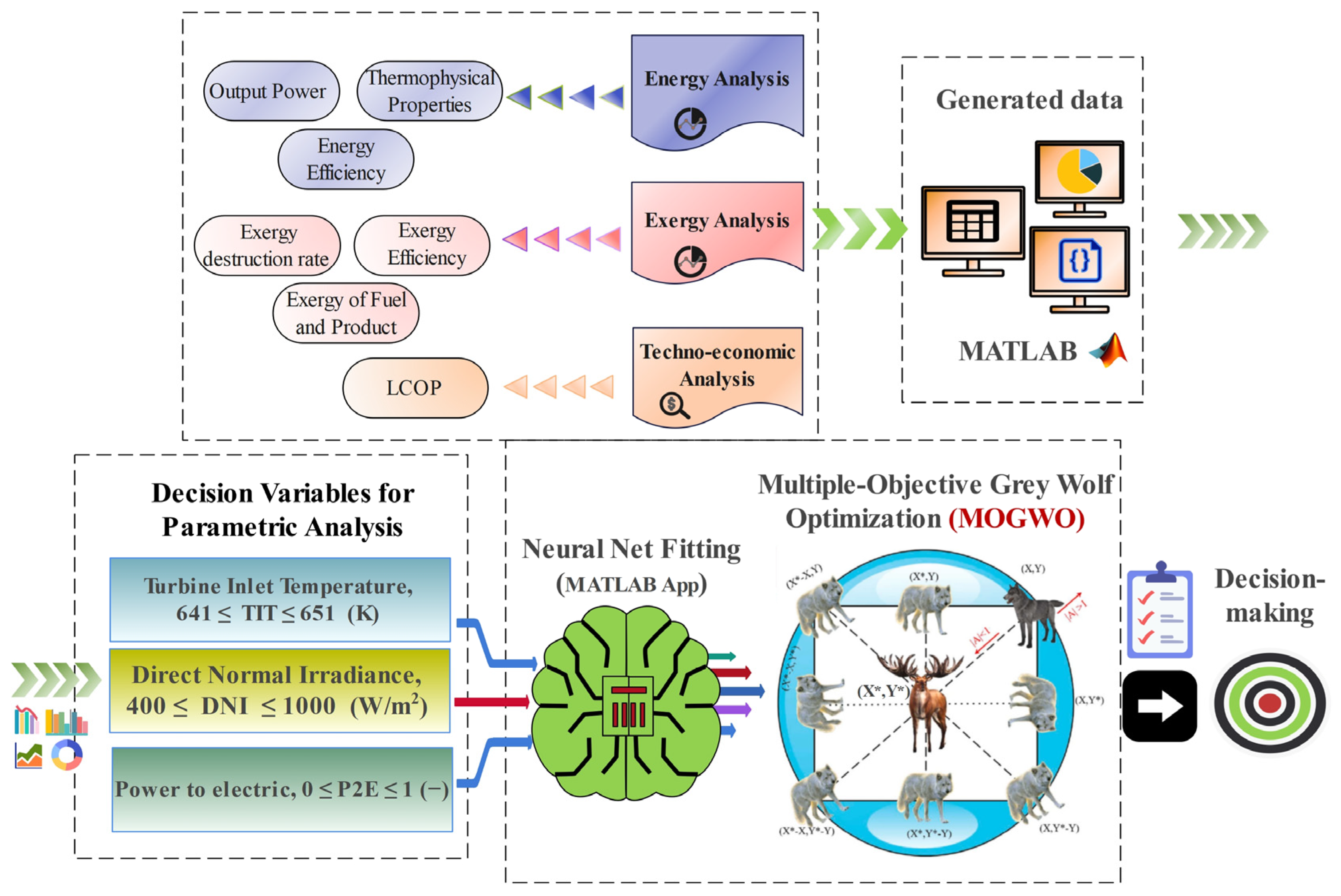
3.5. Multi-Objective Optimization

This paper employs the Multi-Objective Grey Wolf Optimizer (MOGWO) method for optimization. The optimization procedure followed in this study is illustrated in Figure 2. Two optimization scenarios are examined, focusing on the decision-making parameters of direct normal irradiance (DNI), turbine inlet temperature, and P2E. In the first scenario, the objective functions include energy efficiency, exergy efficiency, and levelized cost of production (LCOP). In the second scenario, the objective functions analyzed are water production rate, hydrogen production rate, and LCOP.

3.6. Validation

This section presents the validation of the main subsystems of the proposed configuration using data available in the literature. The results for the RO unit are compared with the simulation data reported in [22] to ensure accuracy. Similarly, the validity of the PEME model is assessed by comparing the simulation results from this study with those presented in [19]. The validation of the remaining subsystems is discussed in detail in the subsequent sections.

3.6.1. ORC

The results of the ORC simulation in this study are compared to the simulation of the RE-TCRC configuration which is thoroughly analyzed by Meng et al. [27]. To verify the validity of our modeling, the energy efficiency values at different turbine inlet pressures for various turbine inlet temperatures are compared and illustrated in Figure 3. Possible sources of error in the ORC validation include numerical approximation errors from differences in simulation methods and data extraction inaccuracies when digitizing reference data. Despite these factors, the overall agreement between the simulation and reference data supports the model’s validity.

3.6.2. PTSC

The validity of the PTSC model employed in this work is assessed by comparing its various parameters to the experimental results reported by Dudley et al. [28] and the simulation results of Okonkwo et al. [21]. The results from experimental tests conducted at Sandia National Laboratory (SNL) are documented in [29] and the values from [25] are simulation results based on these test conditions. Syltherm-800 is utilized as the heat transfer fluid to test a module of the LS-2 collector under various weather conditions, presented as tests 1–8 in

Table 3. Validation of present PTSC model by comparing thermal efficiency to reference simulation study and SNL experimental test cases.

Test	${\mathit{\eta }}_{\mathit{t}\mathit{h}\mathit{e}\mathit{r}\mathit{m}\mathit{a}\mathit{l}} \left(\mathit{\%}\right)$
Cases	Present Study	Okonkwo et al. [21]	Error (%)	Experiment of Dudley et al. [28]	Error (%)
1	0.722	0.707	2.0	0.725	0.48
2	0.716	0.695	3.0	0.709	0.95
3	0.711	0.686	3.6	0.702	1.3
4	0.703	0.668	5.2	0.703	0.057
5	0.699	0.664	5.3	0.680	2.9
6	0.695	0.653	6.5	0.689	0.89
7	0.689	0.636	8.3	0.638	7.9
8	0.687	0.633	8.5	0.633	8.4

. The simulation is conducted in MATLAB (R2021b), utilizing the Coolprop database to acquire the thermodynamic parameters of the heat transfer fluid used in the reference work and with the conditions of the cases as inputs. As shown in Table 3 and

Table 4. Validation of present PTSC model by comparing outlet temperature to reference studies.

Test	${\mathit{T}}_{\mathit{o}\mathit{u}\mathit{t}}$
Cases	Present Study	Okonkwo et al. [21]	Error (%)	Experiment of Dudley et al. [28]	Error (%)
1	398.4	397.2	0.30	397.2	0.30
2	447.8	446.4	0.32	446.5	0.29
3	493.9	492.7	0.24	492.7	0.24
4	542.9	541.4	0.28	542.6	0.062
5	590.2	589.9	0.059	589.6	0.11
6	590.1	589.6	0.091	590.4	0.044
7	647.1	646.9	0.03	647.2	0.016
8	670.83	670.6	0.034	671.2	0.055

, the collector outlet temperatures and energy efficiencies of the collectors correspond well with those documented in other studies. Possible sources of error in the PTSC validation include differences in simulation methods and assumptions between this study and the simulation-based results from Ref. [21]. For the comparison with experimental data from [28], errors may arise from measurement inaccuracies or variations in experimental conditions.

3.6.3. Thermal Storage Tank

To validate the thermal storage model in the present study, the temperature of the thermal storage tank ${(T}_s)$ is compared to the simulation results presented in [29]. Therminol VP-1 is used as the heat transfer fluid and the hourly results for the day with available solar radiation are compared in

Table 5. Comparison of storage tank temperature over the day for present and reference works.

	${\mathit{T}}_{\mathit{s}\mathit{t}} \mathbf{\left(}\mathit{℃}\mathbf{\right)}$
Hour	Present Study	Ashouri et al. [30]	Error (%)
10	109	110	1.0
11	116	115	0.52
12	123	124	0.98
13	133	132	1.3
14	140	139	0.65
15	146	145	0.65
16	150	148	1.0
17	150	150	0.18
18	148	152	2.5
19	145	149	2.2

. Possible sources of error in the validation of the thermal storage tank include minor differences in the mathematical models and equations used in this study and the simulation results from the reference. Despite these factors, the results align well with those obtained in the reference study.

4. Results and Discussion

4.1. Application Considered

Antalya, Turkey, has demonstrated the potential of harvesting energy via solar power systems. Integration of a parabolic trough solar system with a PEME and a reverse osmosis desalination unit for producing electricity, hydrogen, and clean water is proposed, in part due to the high DNI levels and abundant sunny days throughout the year in Antalya. The system uses concentrated solar power to generate heat, which is converted into electricity by an ORC. This electricity powers the PEME, enabling the production of hydrogen through water electrolysis, a key step toward clean fuel generation. Simultaneously, the system utilizes waste heat to enhance the efficiency of the RO desalination unit, supplying clean water. This multi-functional integration showcases an effective and efficient use of solar energy, addressing energy, water, and fuel needs sustainably. The case study also highlights Antalya’s suitability for such innovations, demonstrating a scalable and eco-friendly solution for regions with similar solar resources.

4.2. System Performance and Efficiency

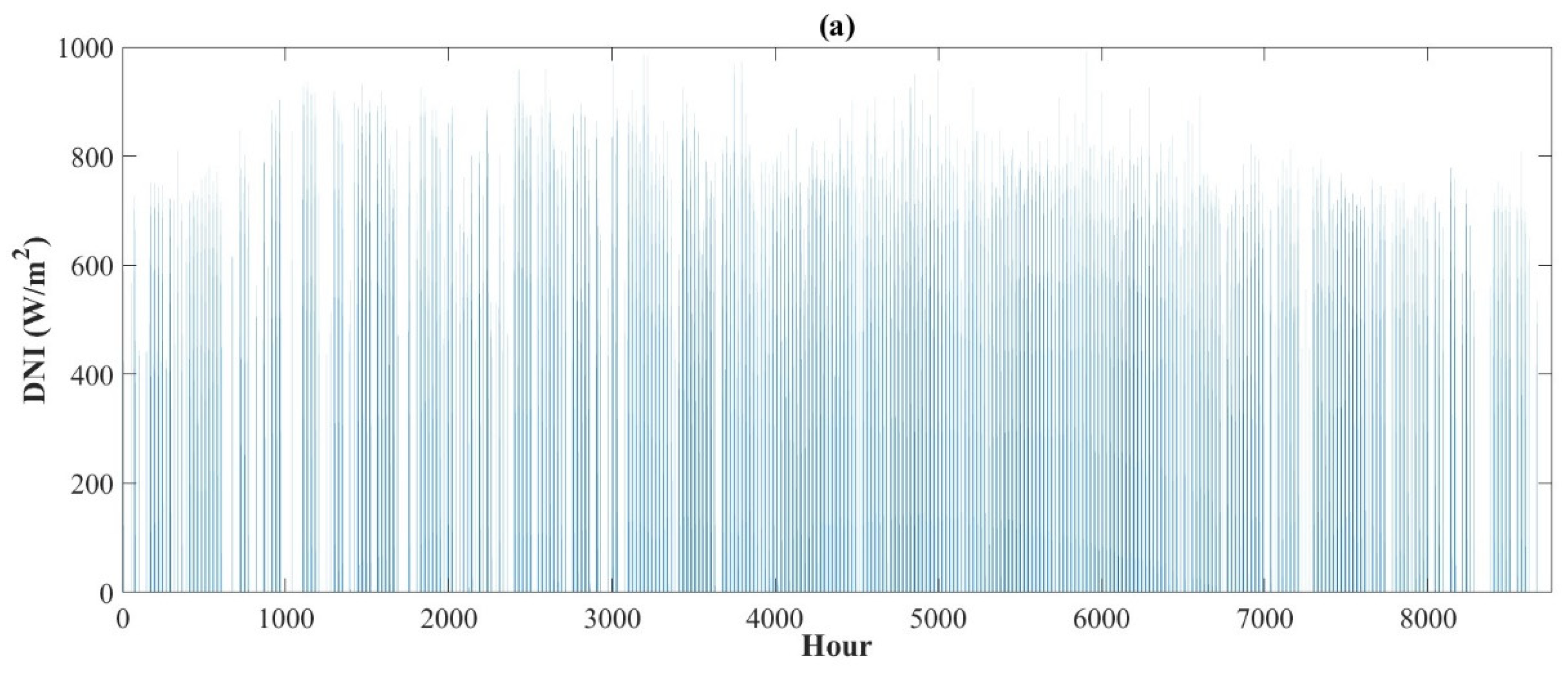
4.2.1. Solar Reservoir

In a parabolic trough system, a reservoir plays a critical role in ensuring the efficient and reliable operation of the solar thermal power plant. It serves as a thermal energy storage unit, enabling the system to store excess heat collected during peak sunlight hours. This stored energy can be utilized during periods of low solar irradiance, such as cloudy days or nighttime, ensuring a continuous energy supply and improving overall grid reliability. The reservoir helps stabilize temperature fluctuations, which enhances the system’s efficiency and lifespan by reducing thermal stress on components. Additionally, it enables better alignment of energy production with demand, increasing the economic viability of parabolic trough systems in renewable energy integration.

Figure 4 shows the number of hours that the reservoir undergoes charge and discharge. It is seen that the amount of time that the tank is charging is much lower than the time spent discharging. The reason for this design is to have a low but consistent power generation rate, hence decreasing the flow rate of the medium to heat the ORC for longer periods of time.

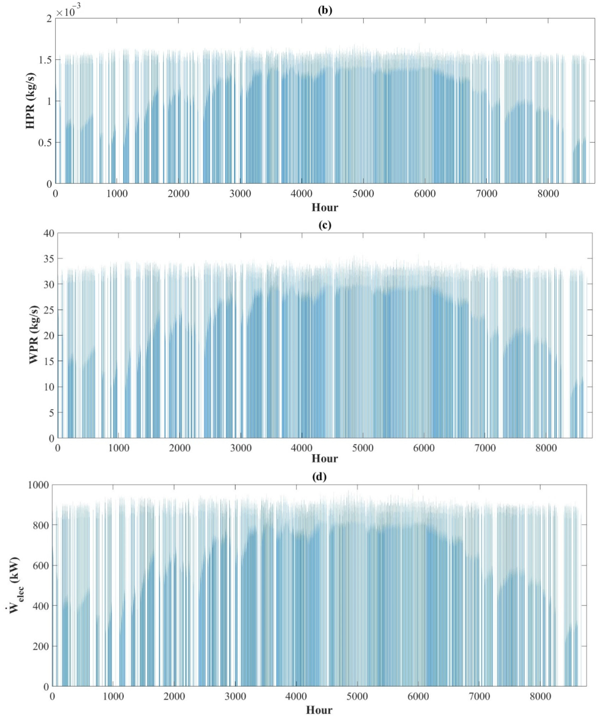
4.2.2. Hourly Distribution of System Production

The dynamic study based on the system presents the distribution of the various parameters of the system in the designated area (Antalya, Turkey). Figure 5a–d show the values of each parameter throughout the year 2020 using Joint Research Centre (JRC) data https://re.jrc.ec.europa.eu (accessed on 5 September 2024). These figures include DNI, generated electricity rate ($\dot{W}$_elec), hydrogen production rate (HPR), and water production rate (WPR) for each hour of the mentioned year. Based on these figures, it is evident that the system’s performance is at a higher level in the summer. Considering the distribution, February shows the most promising DNI values; however, the optimal results presented in other figures are based on the consistent compactness of the DNI values in the summer.

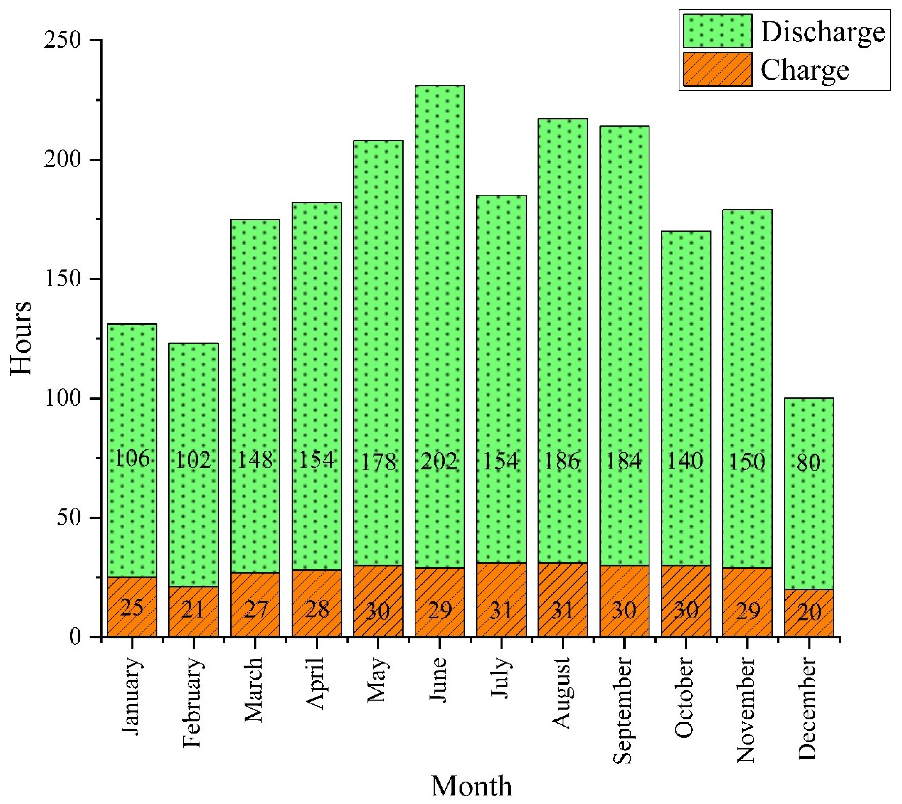
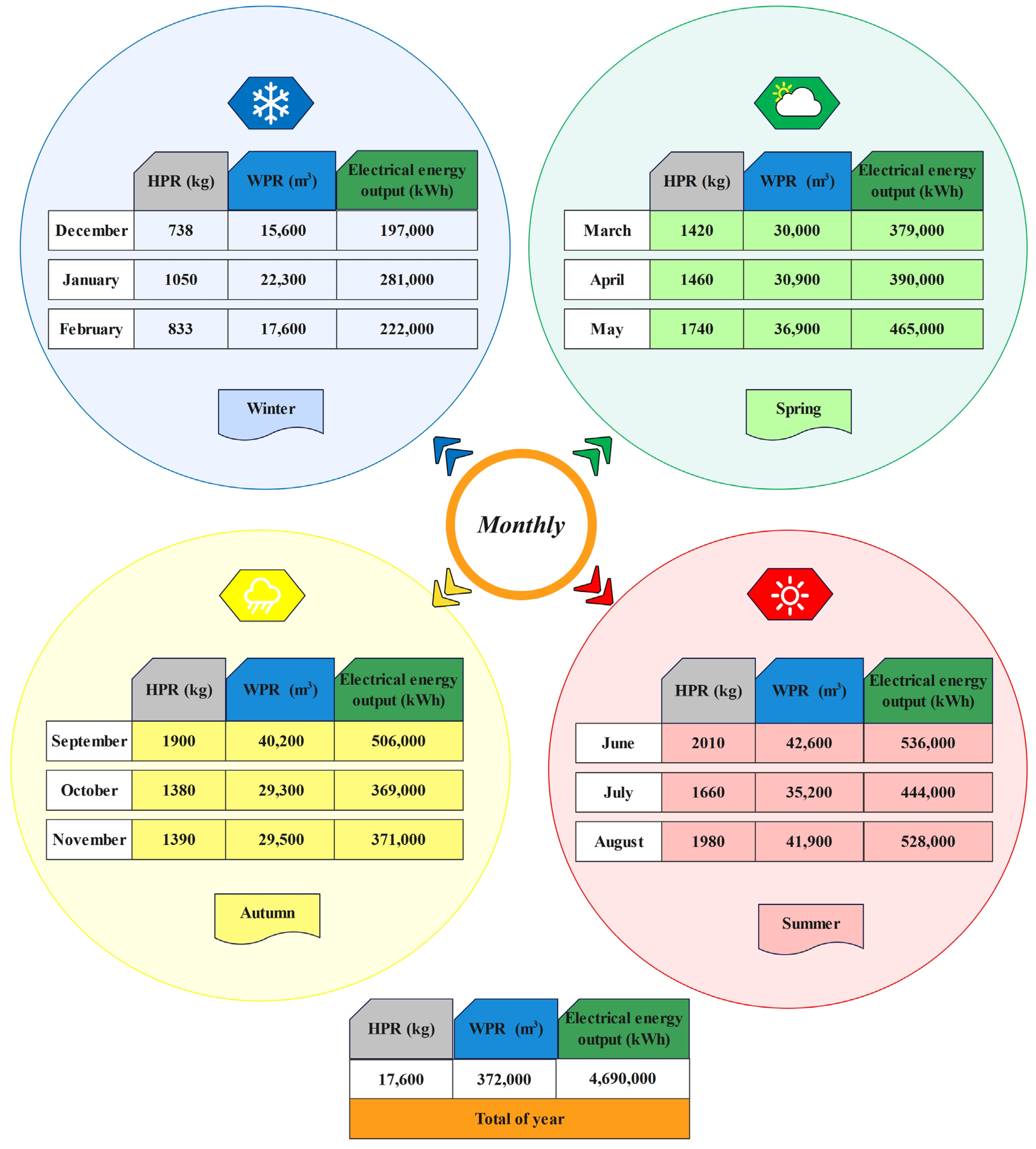
4.2.3. Monthly Distribution of System Products

Figure 6 illustrates the system’s performance for several important parameters: HPR, WPR, and $\dot{W}$_elec, categorized as seasonal and monthly. As seen in this figure, all the parameters mentioned are at their peak value in the summer and the production rates decline significantly in the winter, as expected. As explained in the previous figures, DNI values have the most impactful role in the proposed system’s production rates. June, with production values of 2010 kg of hydrogen, 42,600 m³ of fresh water, and 536,000 kWh of electricity, shows the best performance.

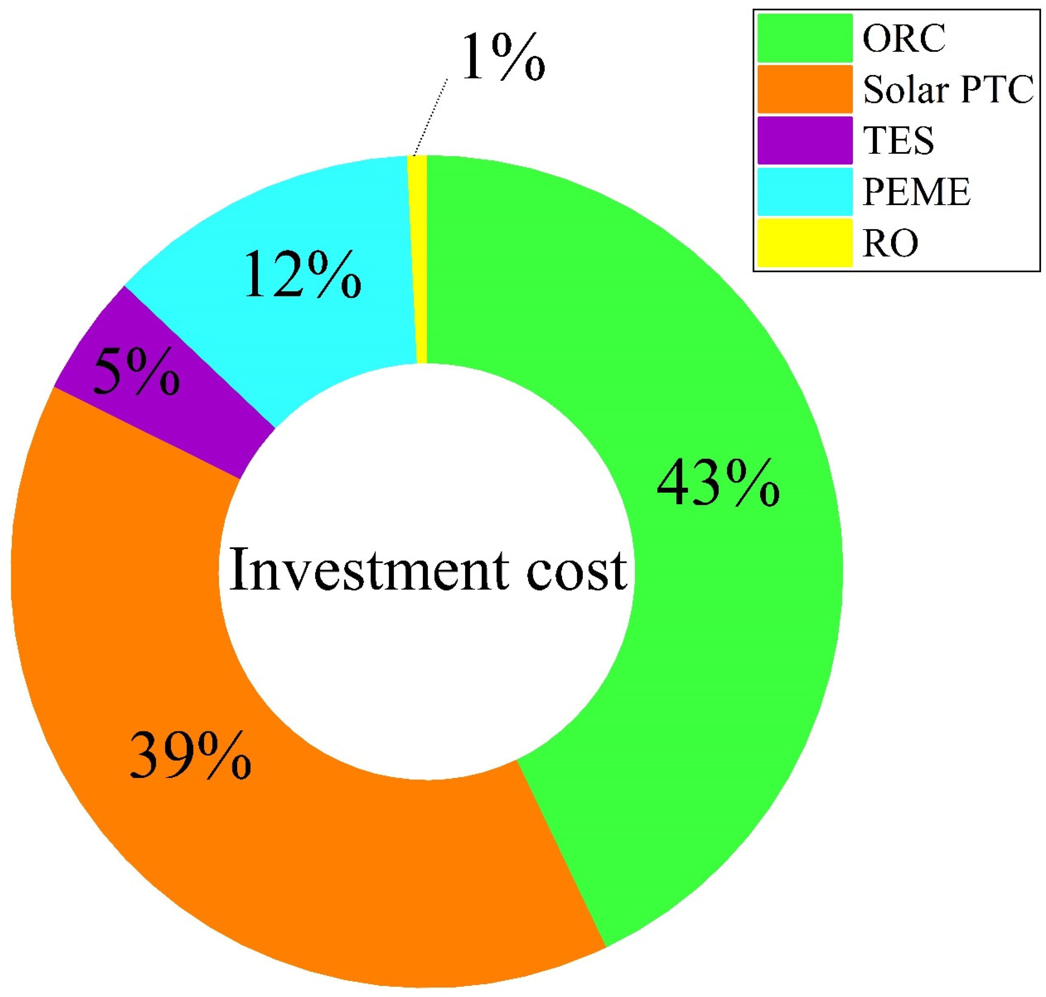
4.2.4. Economic Study of the System

Considering the economic aspects of the designed system from an investment standpoint, the cost is slightly higher for the ORC power production unit than the solar PTC unit. This graph effectively illustrates the economic viability of solar systems based on parabolic trough technology. Based on Figure 7, it is clear that the ORC, the PTC unit, and the PEME require the highest capital investments for the proposed system.

4.2.5. Sankey Diagram of the Multigeneration System

A Sankey diagram for an energy system based on exergy analysis visually presents the flows of energy and its quality across and within the system, emphasizing the usability of energy and its degradation due to irreversibilities. Figure 8 depicts the exergy flows of the media throughout the system based on the entering and exiting exergy values for the components. This figure illustrates the flow rates of exergy and its destruction rates throughout the system. As expected, the parabolic trough, along with the storage tank, has the greatest exergy destruction rates among all the components.

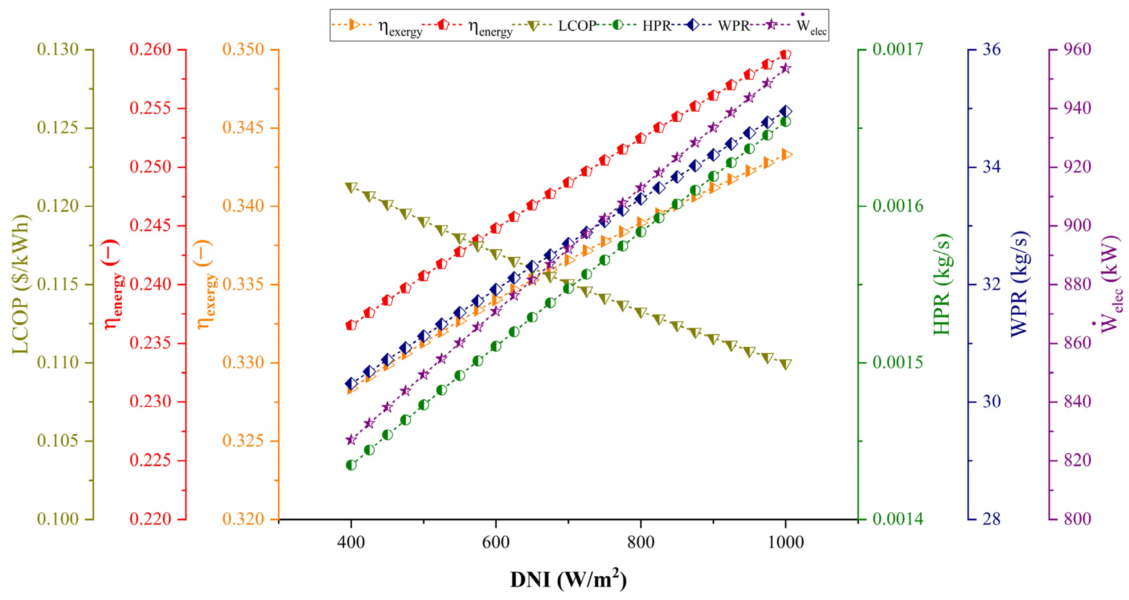
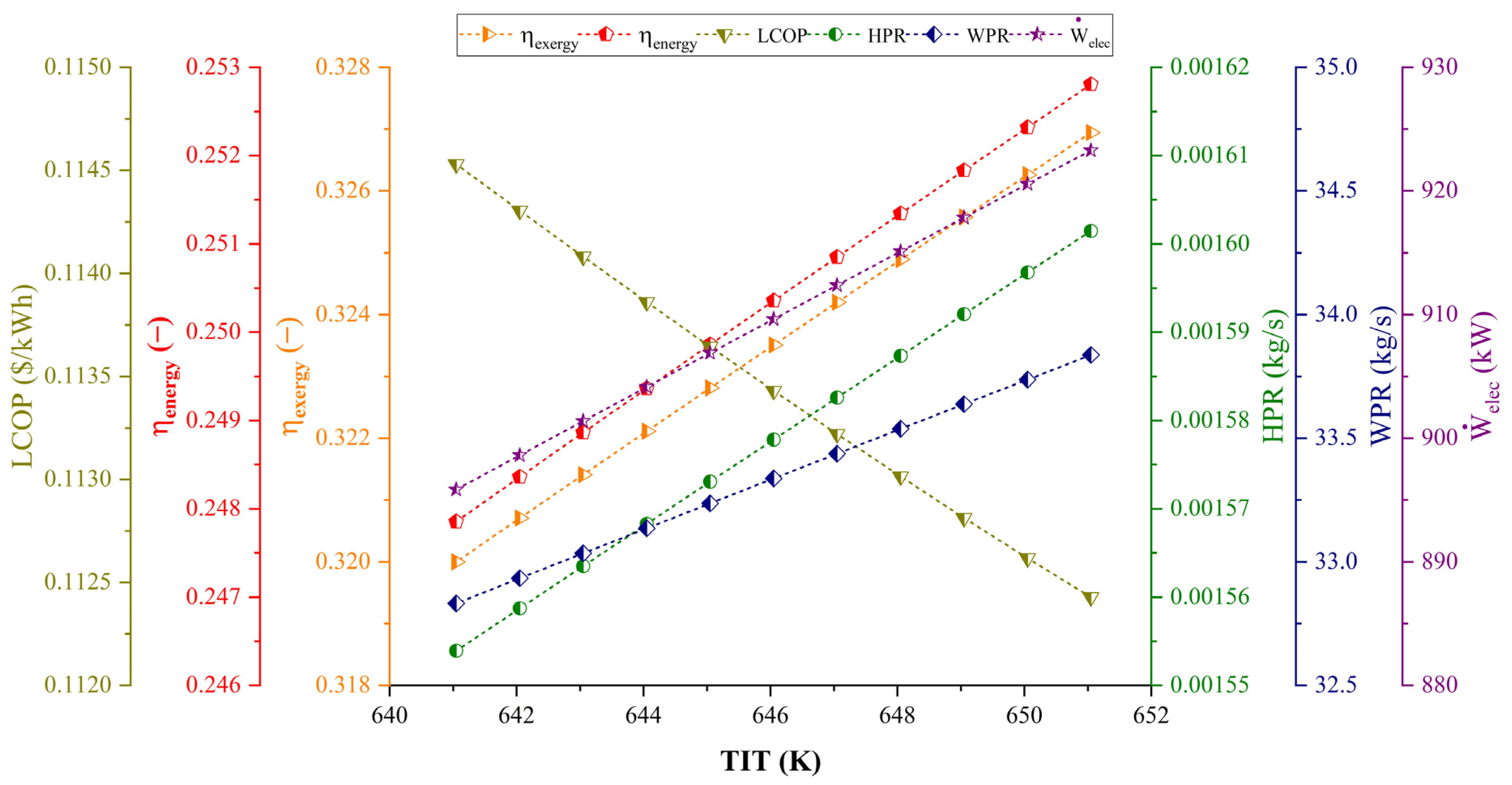
4.3. Parametric Study

A comprehensive parametric study was carried out for the system regarding three important system parameters: DNI for the solar unit, the power cycle’s turbine inlet temperature (TIT), and the rate of power allocated to the grid instead of being used for hydrogen and water generation P2E (P2E).

The impact of DNI on the system’s energy and exergy efficiencies, levelized cost of products (LCOP), HPR, WPR, and $\dot{W}$_elec is displayed in Figure 9. An increase in DNI leads to higher energy and exergy efficiencies because DNI directly correlates with the amount of solar energy captured by the collectors. A higher DNI enhances the receiver’s exposure to more intense solar radiation, which raises the thermal energy input. Since more usable energy is available to convert into electricity, the system’s energy efficiency is increased by this improved thermal input. Since higher temperatures in the heat transfer fluid lessen the irreversibilities in the thermodynamic cycle, especially during heat transfer and power production operations, the exergy efficiency increases concurrently. As a result, at increasing DNI levels, the system functions more closely to its theoretical thermodynamic upper limits.

With an increase in the system’s power production and efficiency, HPR and WPR increase. Also, LCOP decreases as DNI rises because of the elevation in the system’s overall performance indicators such as production rates. Going from a DNI of 400 to a DNI of 1000 W/m², energy and exergy efficiencies, $\dot{W}$_elec, HPR, and WPR increase by around 9.2%, 5.2%, 13%, 14%, and 12.8%, respectively, while LCOP declines by 9%.

Figure 10 illustrates the impact of TIT on the system’s energy and exergy efficiencies, LCOP, HPR, WPR, and $\dot{W}$_elec. Higher turbine inlet temperatures lead to a greater enthalpy drop across the turbine, which increases the work output relative to the heat input, thereby raising the energy efficiency. Additionally, the regeneration process, which recycles heat from the turbine’s exhaust to preheat the working fluid, becomes more effective at higher temperatures, reducing energy losses. From an exergy perspective, higher turbine inlet temperatures increase the quality of the heat supplied, as it more closely matches the working fluid’s ideal temperature profile. This reduces irreversibilities associated with heat transfer and enhances the ability of the system to convert the supplied thermal energy to useful work. Consequently, the system operates closer to its theoretical limits, improving both energy and exergy efficiencies and power production.

As described in the previous figure, with an increase in the system’s power production, the hydrogen and fresh water production, as well as the electricity transmitted to the grid, rise, and, consequently, LCOP decreases. As TIT increases from 641 K to 651 K, the energy and exergy efficiencies, $\dot{W}$_elec, HPR, and WPR increase by around 2.0%, 2.1%, 2.2%, 3.1%, and 3.0%, respectively, while LCOP decreases by 1.8%.

Figure 11 shows the percentage of generated power allocated to the electricity produced for the grid as opposed to being allocated to hydrogen and water production. As can be seen, this allocation has a notable impact on the system’s overall performance and production rates of hydrogen and fresh water. It is clear that electricity generation is more beneficial in terms of energy and exergy efficiencies and LCOP. However, as mentioned earlier, generated power is the prominent factor indicating thermodynamic performance. Therefore, allocating more power for hydrogen and clean water production results in a decrease in the system’s energy and exergy efficiencies. This figure shows the significance of balancing power generation, as well as other demand-based commodities, which is described in the optimization section.

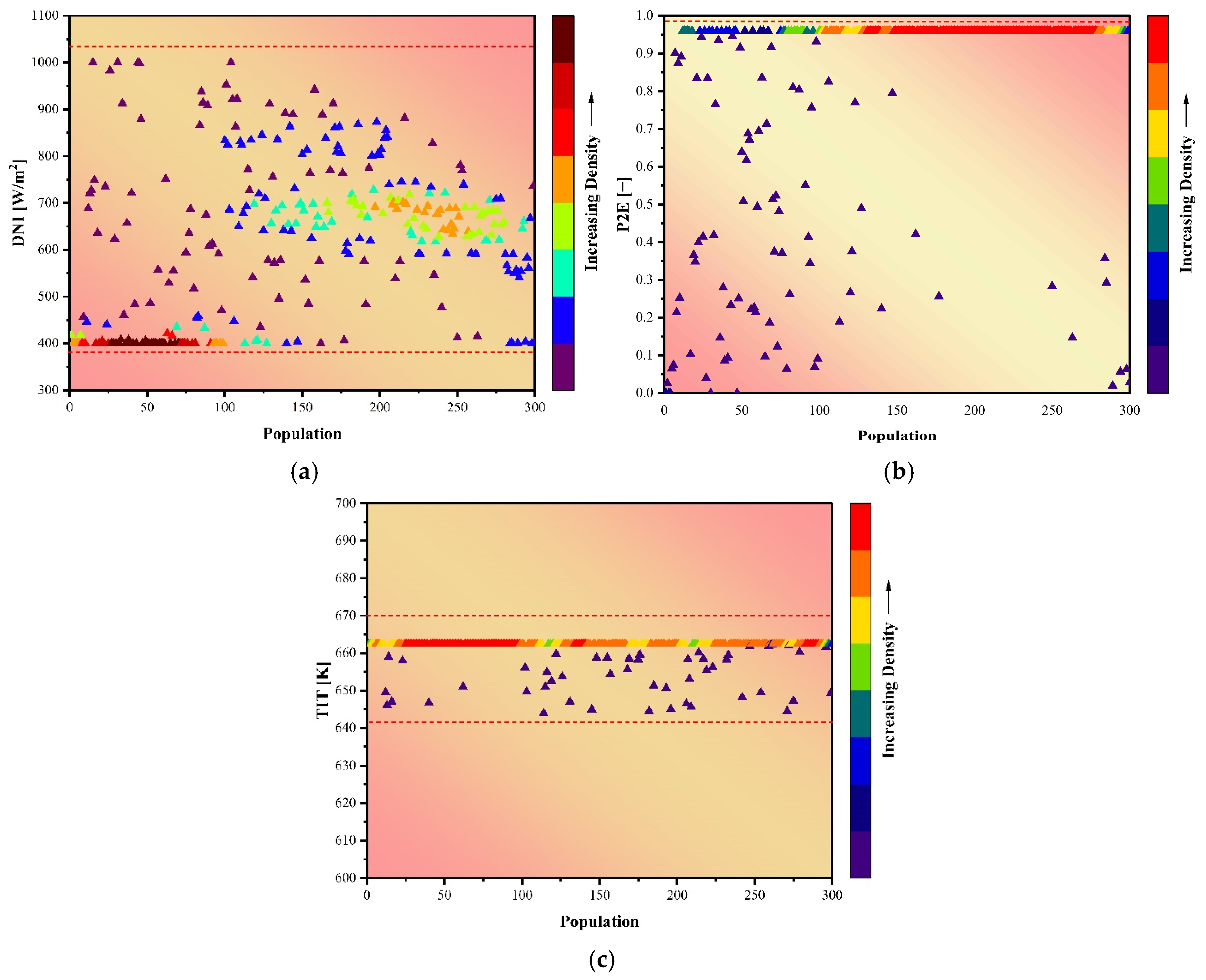
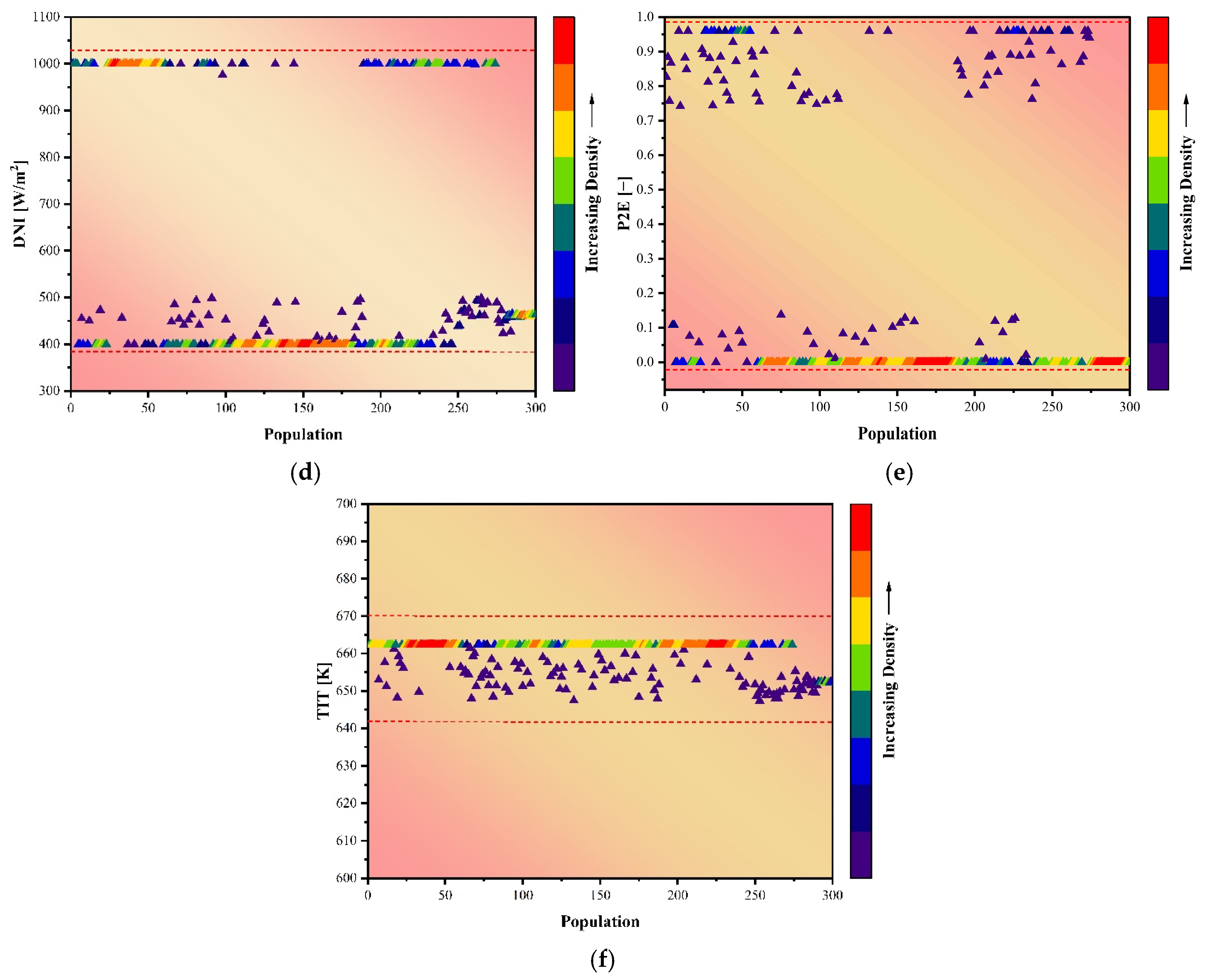
4.4. Optimization Procedure

Machine learning concepts can be applied to the optimization domain to improve the pursuit of the best answers. Machine learning techniques can be used to evaluate data to find patterns and inform decisions. The steps in the optimization process are data collection, preprocessing, feature engineering, model training, and the use of optimization techniques such as the “Grey Wolf algorithm,” in addition to performance evaluation and iterative improvement. This integration facilitates data-driven decision-making.

In this section, the optimization results are discussed to determine the optimal values for three key parameters: direct normal irradiance (DNI) for the solar unit, the power cycle’s turbine inlet temperature (TIT), and the rate of power allocated to the grid instead of being used for hydrogen and water generation (P2E). As illustrated in Figure 2, the optimization process begins with generating data for the levelized cost of power (LCOP), energy efficiency, exergy efficiency, water production ratio (WPR), and hydrogen production ratio (HPR) in two distinct scenarios. Following this, the scatter distribution of the obtained data for each scenario is analyzed to determine the optimal values for each key parameter.

Initially, a dataset was generated using Engineering Equation Solver (EES), considering multiple parameter permutations to examine their influence on system efficiency and product generation. The generated data were then processed in MATLAB, where an artificial neural network (ANN) was trained to model the relationships between these parameters. The trained ANN was subsequently utilized in the Multi-Objective Grey Wolf Optimizer (MOGWO) to determine the optimal parameter set.

The Pareto frontier graphs, presented in Figure 12a,b, illustrate the trade-offs among competing objectives in the optimization process. In the first scenario (Figure 12a), the optimal results were achieved for specific values of energy efficiency (26.5%), exergy efficiency (28.5%), and LCOP (0.106 $/kWh). In the second scenario (Figure 12b), the optimal values were found for specific values of WPR (89.9 kg/s), HPR (0.0062 kg/s), and LCOP (0.11 $/kWh).

The scatter distribution of parameter values is depicted in Figure 13a–f. For the first scenario, Figure 13a–c show that DNI primarily ranges from 400 to 1000 W/m² but clusters more densely around 601.5 W/m². P2E is most frequently observed at 0.98, and TIT is concentrated around 663 K. In the second scenario, Figure 13d–f indicate that DNI is bounded by two key values: 407 W/m² and 992 W/m². P2E is more concentrated around 0.049, contrasting with the first scenario, while TIT remains at 662 K. These results clearly demonstrate the optimum values for each parameter in both scenarios.

5. Conclusions

A solar-powered multigeneration system utilizing a parabolic trough solar collector and a thermal energy storage unit is assessed and optimized. The system consists of a regenerative organic Rankine cycle that generates electricity, which is transmitted to the grid, as well as to the PEM electrolyzer and the reverse osmosis unit to produce hydrogen and clean water, respectively. The thermal energy storage unit allows the system to retain a portion of the solar energy for operation during periods of inadequate or absent solar irradiation, hence extending the system’s operational duration. The proposed system is evaluated from the perspectives of energy, exergy, and economics. DNI, the inlet temperature of the ORC turbine, and the ratio of generated power delivered to the RO and PEME units are identified as important parameters for influencing system performance, and a comprehensive parametric study is carried out on these factors. The feasibility of the proposed system is evaluated considering actual meteorological and solar data from Antalya, Turkey, collected hourly over the course of a year. Also, the MOGWO is implemented to optimize system performance for thermodynamic and economic efficiency.

The primary conclusions of the study are as follows:

• Reduced LCOP and enhanced energy and exergy efficiencies, as well as elevated rates of power, hydrogen, and water generation, are attained with increasing values of DNI and TIT. Also, allocating more electricity to the PEME and RO units decreases the system’s energy and exergy efficiencies and increases LCOP.
• The analysis of the system’s investment costs indicates that the ORC has the highest capital cost. Also, the thermal storage tank constitutes a relatively significant portion of the total costs.
• Under optimal conditions for optimizing production rates and lowering product costs through multi-objective system optimization, the values attained are 89.9 kg/s for WPR, 0.006 kg/s for HPR, and 0.11 $/kWh for LCOP.
• Future work could focus on addressing the practical feasibility of the proposed system, including detailed economic analyses, engineering constraints, and optimization strategies for large-scale implementation. Additionally, incorporating real-world factors such as energy storage, system integration, and operational flexibility could enhance the overall performance and viability of the system. Exploring hybrid configurations or alternative energy sources to complement the existing system could also lead to more sustainable and economically viable solutions in the long term.

References

1. Gul, E.; Baldinelli, G.; Bartocci, P.; Shamim, T.; Domenighini, P.; Cotana, F.; Wang, J.; Fantozzi, F.; Bianchi, F. Transition toward net zero emissions—Integration and optimization of renewable energy sources: Solar, hydro, and biomass with the local grid station in central Italy. Renew. Energy 2023, 207, 672–686. [Google Scholar] [CrossRef]
2. Zabat, L.H.; Sadaoui, N.A.; Abid, M.; Sekrafi, H. Threshold effects of renewable energy consumption by source in U.S. economy. Electr. Power Syst. Res. 2022, 213, 108669. [Google Scholar] [CrossRef]
3. Akan, T. Can renewable energy mitigate the impacts of inflation and policy interest on climate change? Renew. Energy 2023, 214, 255–289. [Google Scholar] [CrossRef]
4. Sarabchi, N.; Mahmoudi, S.M.S.; Yari, M.; Farzi, A. Exergoeconomic analysis and optimization of a novel hybrid cogeneration system: High-temperature proton exchange membrane fuel cell/Kalina cycle, driven by solar energy. Energy Convers. Manag. 2019, 190, 14–33. [Google Scholar] [CrossRef]
5. Wang, T.; Cao, X.; Jiao, L. PEM water electrolysis for hydrogen production: Fundamentals, advances, and prospects. Carbon Neutrality 2022, 1, 21. [Google Scholar] [CrossRef]
6. Laleh, S.S.; Safarpour, A.; Shahrak, A.S.; Alavi, S.H.F.; Soltani, S. Thermodynamic and exergoeconomic analyses of a novel biomass-fired combined cycle with solar energy and hydrogen and freshwater production in sports arenas. Int. J. Hydrogen Energy 2024, 59, 1507–1517. [Google Scholar] [CrossRef]
7. Raninga, M.; Mudgal, A.; Patel, V.; Patel, J. Zeotropic mixture as a working fluid for cascade Rankine cycle-based reverse osmosis: Energy, exergy, and economic analysis. Int. J. Thermofluids 2024, 24, 100890. [Google Scholar] [CrossRef]
8. Batista, N.E.; Carvalho, P.C.M.; Fernández-Ramírez, L.M.; Braga, A.P.S. Optimizing methodologies of hybrid renewable energy systems powered reverse osmosis plants. Renew. Sustain. Energy Rev. 2023, 182, 113377. [Google Scholar] [CrossRef]
9. Kolathur, S.; Khatiwada, D.; Khan, E.U. Life cycle assessment and life cycle costing of a building-scale, solar-driven water purification system. Energy Nexus 2023, 10, 100208. [Google Scholar] [CrossRef]
10. Zheng, N.; Zhang, H.; Duan, L.; Wang, Q.; Bischi, A.; Desideri, U. Techno-economic analysis of a novel solar-driven PEMEC-SOFC-based multi-generation system coupled parabolic trough photovoltaic thermal collector and thermal energy storage. Appl. Energy 2023, 331, 120400. [Google Scholar] [CrossRef]
11. Zheng, N.; Zhang, H.; Duan, L.; Wang, X.; Liu, L. Energy, exergy, exergoeconomic and exergoenvironmental analysis and optimization of a novel partially covered parabolic trough photovoltaic thermal collector based on life cycle method. Renew. Energy 2022, 200, 1573–1588. [Google Scholar] [CrossRef]
12. Bedakhanian, A.; Maleki, A.; Haghighat, S. Utilizing the multi-objective particle swarm optimization for designing a renewable multiple energy system on the basis of the parabolic trough solar collector. Int. J. Hydrogen Energy 2022, 47, 36433–36447. [Google Scholar] [CrossRef]
13. Zhang, Y.; Ma, S.; Yue, W.; Tian, Z.; Yang, C.; Gao, W. Energy; exergy, economic and environmental (4E) evaluation of a solar-integrated energy system at medium–high temperature using CO2 as the parabolic trough collector (PTC) working medium. Energy Convers. Manag. 2023, 296, 117683. [Google Scholar] [CrossRef]
14. Maya, J.C.; Chejne, F.; Gómez, C.A.; Montoya, J.; Chaquea, H.; Pecha, B. Analysys of the performance a PEM-type electrolyzer in variable energy supply conditions. Chem. Eng. Res. Des. 2023, 196, 526–541. [Google Scholar] [CrossRef]
15. Abdollahipour, A.; Sayyaadi, H. Optimal design of a hybrid power generation system based on integrating PEM fuel cell and PEM electrolyzer as a moderator for micro-renewable energy systems. Energy 2022, 260, 124944. [Google Scholar] [CrossRef]
16. Astriani, Y.; Tushar, W.; Nadarajah, M. Optimal planning of renewable energy park for green hydrogen production using detailed cost and efficiency curves of PEM electrolyzer. Int. J. Hydrogen Energy 2024, 79, 1331–1346. [Google Scholar] [CrossRef]
17. Abedi, M.; Tan, X.; Klausner, J.F.; Bénard, A. Solar desalination chimneys: Investigation on the feasibility of integrating solar chimneys with humidification–dehumidification systems. Renew. Energy 2023, 202, 88–102. [Google Scholar] [CrossRef]
18. Kianfard, H.; Khalilarya, S.; Jafarmadar, S. Exergy and exergoeconomic evaluation of hydrogen and distilled water production via combination of PEM electrolyzer, RO desalination unit and geothermal driven dual fl uid ORC. Energy Convers. Manag. 2018, 177, 339–349. [Google Scholar] [CrossRef]
19. Dashtizadeh, E.; Darestani, M.M.; Rostami, S.; Ashjaee, M.; Houshfar, E. Comparative optimization study and 4E analysis of hybrid hydrogen production systems based on PEM, and VCl methods utilizing steel industry waste heat. Energy Convers. Manag. 2024, 303, 118141. [Google Scholar] [CrossRef]
20. Al-Sulaiman, F.A.; Hamdullahpur, F.; Dincer, I. Performance assessment of a novel system using parabolic trough solar collectors for combined cooling, heating, and power production. Renew. Energy 2012, 48, 161–172. [Google Scholar] [CrossRef]
21. Okonkwo, E.C.; Essien, E.A.; Akhayere, E.; Abid, M.; Kavaz, D.; Ratlamwala, T.A.H. Thermal performance analysis of a parabolic trough collector using water-based green-synthesized nanofluids. Sol. Energy 2018, 170, 658–670. [Google Scholar] [CrossRef]
22. Blanco-Marigorta, A.M.; Masi, M.; Manfrida, G. Exergo-environmental analysis of a reverse osmosis desalination plant in Gran Canaria. Energy 2014, 76, 223–232. [Google Scholar] [CrossRef]
23. Abbasi, H.R.; Pourrahmani, H. Multi-criteria optimization of a renewable hydrogen and freshwater production system using HDH desalination unit and thermoelectric generator. Energy Convers. Manag. 2020, 214, 112903. [Google Scholar] [CrossRef]
24. Al-Sulaiman, F.A.; Dincer, I.; Hamdullahpur, F. Exergy modeling of a new solar driven trigeneration system. Sol. Energy 2011, 85, 2228–2243. [Google Scholar] [CrossRef]
25. Wang, J.; Dai, Y.; Gao, L.; Ma, S. A new combined cooling, heating and power system driven by solar energy. Renew. Energy 2009, 34, 2780–2788. [Google Scholar] [CrossRef]
26. Gao, Z.; Miao, J.; Zhao, J.; Mesri, M. Comprehensive economic analysis and multi-objective optimization of an integrated gasification power generation cycle. Process Saf. Environ. Prot. 2021, 155, 61–79. [Google Scholar] [CrossRef]
27. Meng, F.; Wang, E.; Zhang, B.; Zhang, F.; Zhao, C. Thermo-economic analysis of transcritical CO2 power cycle and comparison with Kalina cycle and ORC for a low-temperature heat source. Energy Convers. Manag. 2019, 195, 1295–1308. [Google Scholar] [CrossRef]
28. Dudley, V.E.; Kolb, J.; Mahoney, A.R.; Mancini, T.R.; Matthews, C.W. Test Results of SEGS LS-2 Solar Collector; USDOE: Washington, DC, USA, 1994.
29. Ashouri, M.; Vandani, A.M.K.; Mehrpooya, M.; Ahmadi, M.H.; Abdollahpour, A. Techno-economic assessment of a Kalina cycle driven by a parabolic Trough solar collector. Energy Convers. Manag. 2015, 105, 1328–1339. [Google Scholar] [CrossRef]
30. Kurşun, B.; Ökten, K. Comprehensive energy; exergy, and economic analysis of the scenario of supplementing pumped thermal energy storage (PTES) with a concentrated photovoltaic thermal system. Energy Convers. Manag. 2022, 260, 115592. [Google Scholar] [CrossRef]
31. Boyaghchi, F.A.; Chavoshi, M. Multi-criteria optimization of a micro solar-geothermal CCHP system applying water/CuO nanofluid based on exergy, exergoeconomic and exergoenvironmental concepts. Appl. Therm. Eng. 2017, 112, 660–675. [Google Scholar] [CrossRef]
32. Hai, T.; Kumar, A.; Aminian, S.; Al-Qargholi, B.; Soliman, N.F.; El-Shafai, W. Improved efficiency in an integrated geothermal power system including fresh water unit: Exergoeconomic analysis and dual-objective optimization. Process Saf. Environ. Prot. 2023, 180, 305–323. [Google Scholar] [CrossRef]
33. Fan, G.; Yang, B.; Guo, P.; Lin, S.; Farkoush, S.G.; Afshar, N. Comprehensive analysis and multi-objective optimization of a power and hydrogen production system based on a combination of flash-binary geothermal and PEM electrolyzer. Int. J. Hydrogen Energy 2021, 46, 33718–33737. [Google Scholar] [CrossRef]
34. Khodaei, E.; Yari, M.; Nami, H.; Goravanchi, F. Techno-economic Assessment and Optimization of a Solar-Driven Power and Hydrogen Co-generation Plant Retrofitted with Enhanced Energy Storage. Energy Convers. Manag. 2024, 301, 118004. [Google Scholar] [CrossRef]
Figure 1. Schematic of the solar-energy-driven multigeneration plant.
Sustainability 17 03555 g001
Figure 2. Flowchart of the optimization procedure conducted in this study.
Sustainability 17 03555 g002
Figure 3. Comparison of energy efficiency values of ORCs for varying turbine inlet pressures in the present study and the reference work.
Sustainability 17 03555 g003
Figure 4. Monthly distribution of charging and discharging hours of the reservoir tank, showing seasonal variations and indicating higher storage activity during summer months due to increased solar availability.
Sustainability 17 03555 g004
Figure 5. Hourly distribution over the year of four key parameters of the system for the given year: (a) DNI in Antalya, Turkey, (b) hydrogen production rate, (c) fresh water production rate, and (d) electrical power produced. The figure illustrates the strong correlation between solar input and system outputs, underlining the system’s dependence on solar resource availability.
Sustainability 17 03555 g005aSustainability 17 03555 g005b
Figure 6. Monthly and seasonal distribution of three key parameters of the system over the year, emphasizing the system’s seasonal performance variation and its higher productivity in sunnier periods.
Sustainability 17 03555 g006
Figure 7. Breakdown of capital investment by subsystem, indicating major cost contributors and helping to identify areas for potential cost optimization in future implementations.
Sustainability 17 03555 g007
Figure 8. Sankey diagram of the multigeneration system.
Sustainability 17 03555 g008
Figure 9. Impact of DNI on the system’s energy and exergy efficiencies, LCOP (levelized cost of products), HPR, WPR, and W ˙ elec, showing the system’s sensitivity to solar irradiance and its performance scalability in high-sunlight regions.
Sustainability 17 03555 g009
Figure 10. Impact of TIT on the system’s energy and exergy efficiencies, LCOP (levelized cost of products), HPR, WPR, and W ˙ elec, indicating that efficiency and production improve significantly at higher TIT values.
Sustainability 17 03555 g010
Figure 11. Impact of P2E on the system’s energy and exergy efficiencies, LCOP (levelized cost of products), HPR, WPR, and W ˙ elec., demonstrating how optimization of energy distribution between outputs affects overall efficiency and product costs.
Sustainability 17 03555 g011
Figure 12. Optimization results for the multigeneration system. (a) Pareto front of the optimum results for energy efficiency, exergy efficiency, and LCOP and (b) Pareto front of the optimum results for WPR, HPR, and LCOP. The diagram shows the pareto front in red, with the blue, green and purple colors representing the reflections of pareto front on different planes of the coordinate system.
Sustainability 17 03555 g012
Figure 13. (ac) Scatter distribution for the first scenario. (df) Scatter distribution for the second scenario.
Sustainability 17 03555 g013aSustainability 17 03555 g013b