Research on High Spatiotemporal Resolution of XCO₂ in Sichuan Province Based on Stacking Ensemble Learning

Abstract

Global warming caused by the increase in the atmospheric CO₂ content has become a focal environmental issue of common concern to the international community. As a key resource support for achieving the “dual carbon” goals in Western China, Sichuan Province requires a deep analysis of its carbon sources, carbon sinks, and its characteristics in terms of atmospheric environmental capacity, which is of great significance for formulating effective regional sustainable development strategies and responding to global climate change. In view of the unique geographical and climatic conditions in Sichuan Province and the current situation of a low and uneven distribution of atmospheric environmental capacity, this paper uses three forms of multi-source satellite data, OCO-2, OCO-3, and GOSAT, combined with other auxiliary data, to generate a daily XCO₂ concentration dataset with a spatial resolution of a 1km grid in Sichuan Province from 2015 to 2022. Based on the Optuna optimization method with 10-fold cross-validation, the optimal hyperparameter configuration of the four base learners of Stacking, random forest, gradient boosting decision tree, extreme gradient boosting, and the K nearest neighbor algorithm is searched for; finally, the logistic regression algorithm is used as the second-layer meta-learner to effectively improve the prediction accuracy and generalization ability of the Stacking ensemble learning model. According to the comparison of the performance of each model by cross-validation and TCCON site verification, the Stacking model significantly improved in accuracy, with an R², RMSE, and MAE of 0.983, 0.87 ppm and 0.19 ppm, respectively, which is better than those of traditional models such as RF, KNN, XGBoost, and GBRT. The accuracy verification of the atmospheric XCO₂ data estimated by the model based on the observation data of the two TCCON stations in Xianghe and Hefei showed that the correlation coefficients were 0.96 and 0.98, and the MAEs were 0.657 ppm and 0.639 ppm, respectively, further verifying the high accuracy and reliability of the model. At the same time, the fusion of multi-source satellite data significantly improved the spatial coverage of XCO₂ concentration data in Sichuan Province, effectively filling the gap in single satellite observation data. Based on the reconstructed XCO₂ dataset of Sichuan Province, the study revealed that there are significant regional and seasonal differences in the XCO₂ concentrations in the region, showing seasonal variation characteristics of being higher in spring and winter and lower in summer and autumn; in terms of the spatial distribution, the overall spatial distribution characteristics are high in the east and low in the west. This study helps to deepen our understanding of the carbon cycle and climate change, and can provide a scientific basis and risk assessment methods for policy formulation, effect evaluation, and international cooperation.

1. Introduction

As global warming intensifies, carbon emissions have attracted the attention of all countries. Carbon dioxide (CO₂), the main greenhouse gas in the atmosphere, rose from 277 ppm before the start of the industrial era to 420 ppm in 2023 [1], with an increase of 2.1 ppm between 2022 and 2023. Most researchers believe that urban areas are the main source of greenhouse gas emissions. Although they account for less than 3% of the world’s land area, they contribute more than 70% of anthropogenic greenhouse gas emissions. The Paris Agreement clearly stipulates that countries must take voluntary emission reduction measures from 2020, and stipulates that a global carbon inventory assessment will be conducted every five years starting from 2023 [2]. In this context, accurately obtaining high-resolution spatial and temporal distribution data of CO₂ is not only the basis for quantifying urban anthropogenic carbon emissions, but also a necessary condition for formulating and implementing effective carbon reduction strategies [3].

With the continuous development of remote sensing technology, countries have successively launched satellites dedicated to carbon dioxide monitoring, and remote sensing monitoring has gradually become the core means of detecting the atmospheric CO₂ column concentration. Compared with ground stations and air-based platforms, satellite observations have the advantages of a wide coverage, stable and continuous observation time, strong repeatability and high data objectivity, and can provide continuous spatial distribution and dynamic change information of greenhouse gases on a global scale [4,5,6]. Recently, many carbon-sensing satellites have been successfully deployed around the world to monitor the atmospheric CO₂ column concentration, including Europe’s Envisat, Japan’s GOSAT series, the United States’ OCO series, and China’s TanSat [7]. By observing the average dry air mole fraction of the CO₂ column (XCO₂), they provide rich data support for the study of the CO₂ concentration. Most mainstream satellites in the field of carbon dioxide monitoring are equipped with passive detectors and use narrow-band observation modes [8,9]. However, their observations are easily interfered with by various factors such as clouds, aerosols, and surface reflectivity in the atmosphere, resulting in certain limitations in the temporal and spatial coverage and accuracy of satellite data. Therefore, filling the gaps in satellite inversion data is of great significance for obtaining the complete spatiotemporal distribution of XCO₂.

Satellite remote sensing data are widely used in the study of the spatiotemporal distribution of XCO₂ due to their advantages such as good continuity and wide spatial coverage. Currently, geographically weighted regression and machine learning models are common methods for studying the spatiotemporal distribution of atmospheric carbon dioxide. Based on technologies such as Kriging interpolation, random forest model (RF), and extreme gradient boosting (XGBoost), researchers have integrated satellite remote sensing XCO₂ data, meteorological data, and NDVI data to reconstruct the high-coverage spatiotemporal distribution of XCO₂ in the world and China [10,11,12,13]. However, existing regional studies are mostly concentrated in the Beijing–Tianjin–Hebei region [12], Changshanjiao region [14], and the northwest region [15], and rarely involve the southwest region, especially the spatiotemporal distribution of XCO₂ in Sichuan Province, which has not received sufficient attention. Due to differences in the observation period, orbital layout, and inversion technology, each satellite exhibits unique complementary characteristics in terms of spatial coverage. Consequently, combining multi-source satellite data is considered a viable approach to enhance the coverage efficiency of satellite XCO₂ observations. However, this process faces significant challenges, as existing methods struggle to effectively integrate and reconstruct multi-source datasets with high spatiotemporal accuracy. Traditional machine learning algorithms usually rely on a single model, which may cause them to face certain limitations in processing nonlinear or diverse datasets. In contrast, the Stacking ensemble learning algorithm fully utilizes the advantages of different models by integrating the prediction results of multiple base learners, effectively making up for the shortcomings of a single model in processing complex data.

In terms of regional-scale CO₂ monitoring, Wang et al. [12] successfully reconstructed the high-precision daily carbon dioxide column concentration (XCO₂) distribution in the Beijing–Tianjin–Hebei region from 2015 to 2019 using multi-source satellite data and random forest models, revealing its spatial differentiation and seasonal variation characteristics. The performance of their model (R² of 0.96, RMSE of 1.09 ppm, and MAE of 0.56 ppm) verified the effectiveness of this method in regional-scale CO₂ monitoring. In addition, Tang et al. [16] developed a downscaling machine learning model to fill the gap in the inversion data of the Orbital Carbon Observatory-2 satellite in Northeast China from 2018 to 2023, further revealing the spatiotemporal distribution characteristics and growth trend of XCO₂ in the region, and confirming the necessity of downscaling modeling in enhancing the understanding of the carbon cycle. Yao et al. [17] pointed out that during the period of 2018–2021, the average center of China’s XCO₂ migrated westward, especially in the southwest and Qinghai–Tibet Plateau, where the growth rate of XCO₂ was particularly obvious, exceeding that of the eastern region. This trend may be related to the dynamics of terrestrial carbon sources/sinks. Although these studies have made significant progress in regional-scale CO₂ monitoring in China and many provinces, relatively few studies have been conducted on provincial or smaller areas. Therefore, this study takes Sichuan Province, which has unique geographical characteristics, as the research area; obtains OCO-2, OCO-3, and GOSAT multi-source satellite data; and constructs a dataset. Through data fusion and the Stacking ensemble learning algorithm optimized by Optuna, the annual, seasonal, and monthly concentration data of Sichuan Province with high spatial coverage (1 km × 1 km) from 2015 to 2022 are obtained. Taking prefecture-level cities and pixel grids as units, the distribution pattern and spatiotemporal variation trend of the XCO₂ concentration in Sichuan Province are analyzed in time and space to reveal the spatiotemporal distribution characteristics of the XCO₂ concentration in Sichuan Province, and provide new ideas and data support for the province’s refined carbon monitoring and management strategy, thus helping to promote the realization of the “dual carbon” goals.

2. Data and Methods

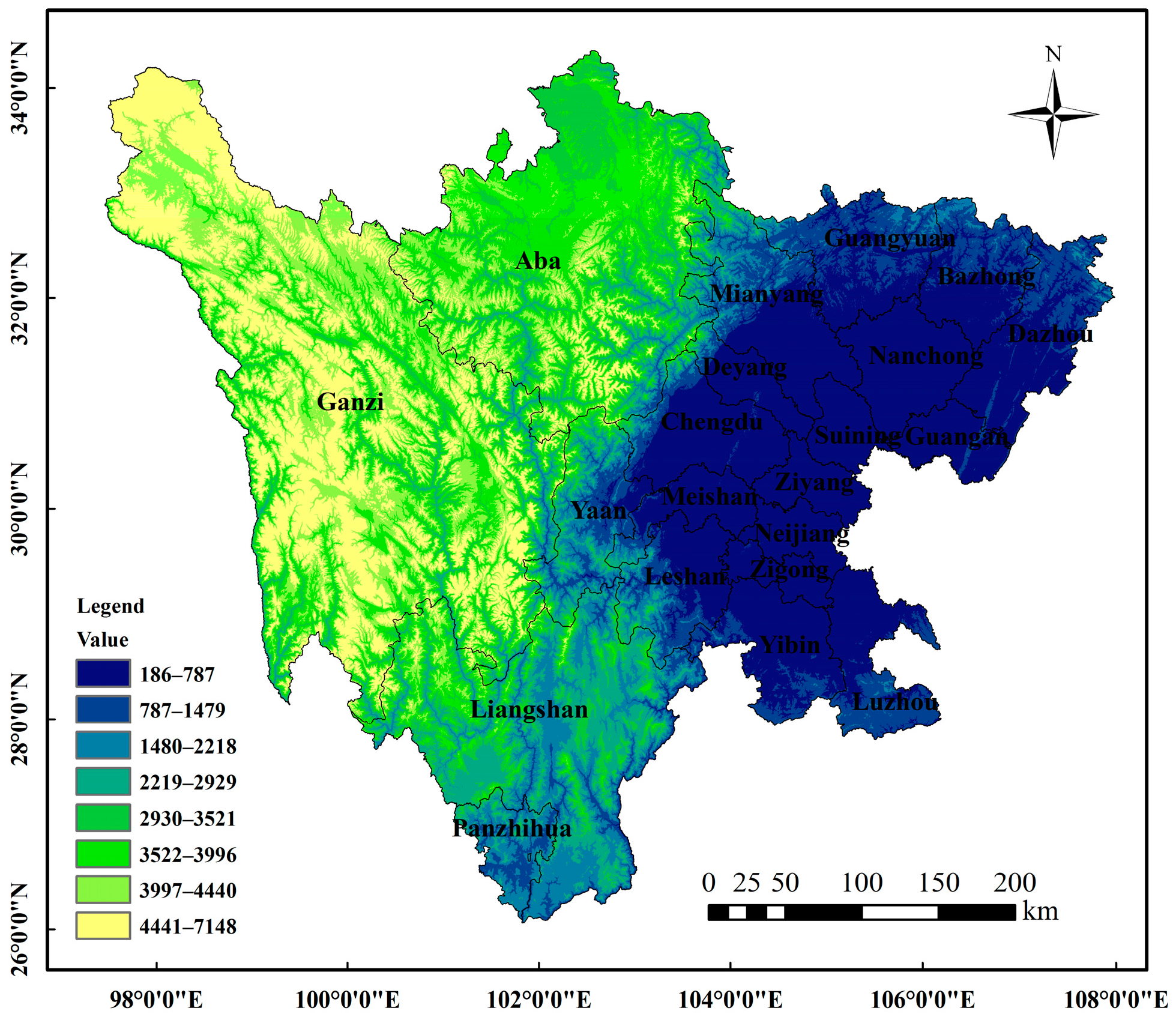
2.1. Overview of the Study Area

Sichuan Province is located at 97°21′–110°12′ E, 26°03′–34°19′ N, with a total area of about 486,000 square kilometers. Sichuan Province, situated in the southwestern interior of China, lies at the transitional zone between the Qinghai–Tibet Plateau and the Yangtze River Plain’s middle and lower reaches. It borders Chongqing to the east, Yunnan and Guizhou to the south, Tibet to the west, and Qinghai, Gansu, and Shaanxi to the north. Renowned as the “Land of Abundance”, it holds significant geographical and ecological importance. The province is geographically divided into three main regions: the Sichuan Basin, the Northwest Sichuan Plateau, and the Southwest Sichuan Mountains. The terrain is characterized by significant differences in height. The west is dominated by plateaus and mountains, with altitudes of more than 4000 m, while the east is a basin and hilly area, with altitudes of 1000 to 3000 m. This study focuses on Sichuan Province (Figure 1), a region characterized by complex topography, diverse landforms, and a dense population. By analyzing and evaluating driving factors related to its natural geography and human activities, this research aims to provide data-driven insights to support low-carbon economic development and urban atmospheric environmental governance in the region.

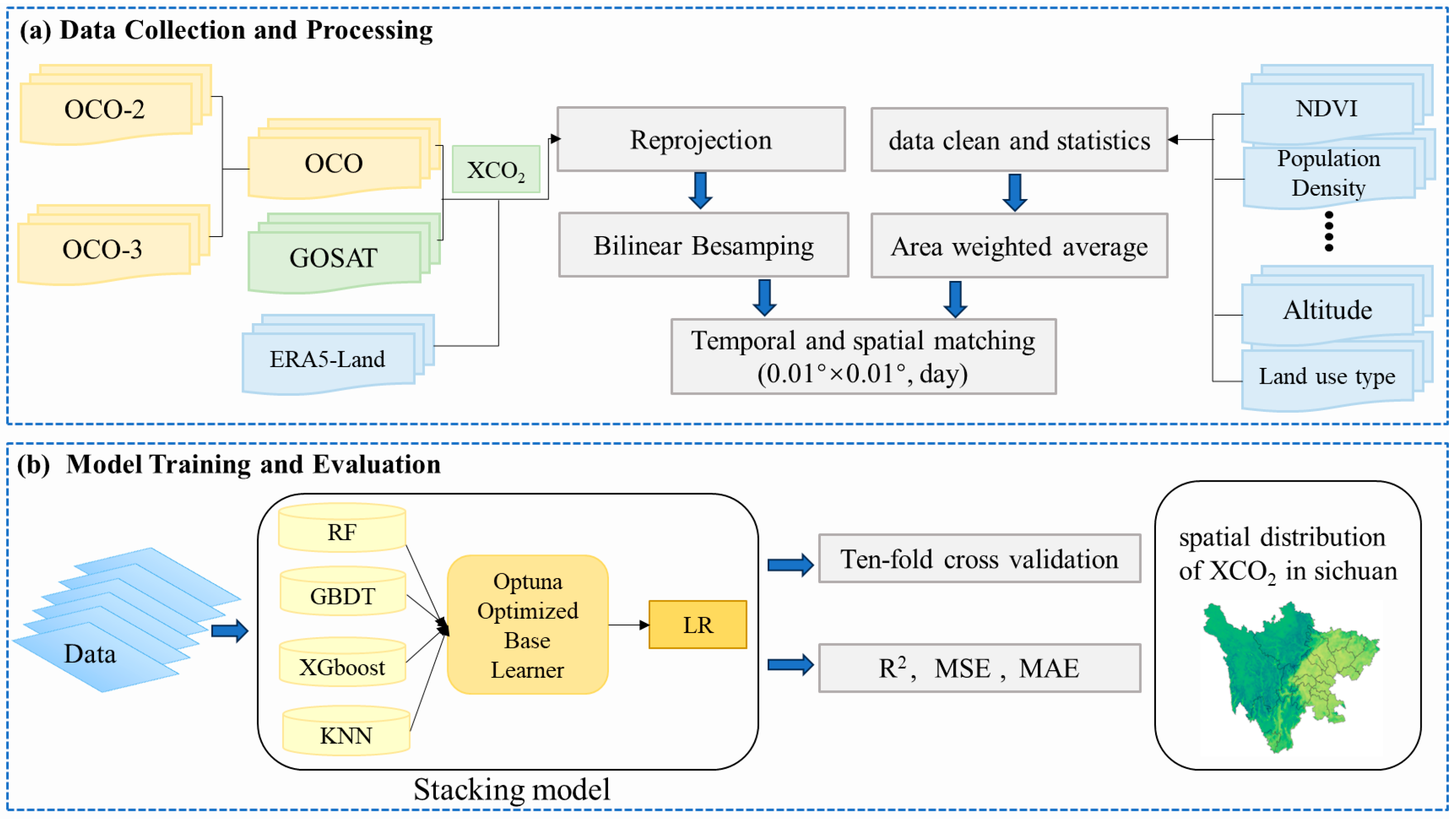
2.2. Data and Processing

This study utilizes the following datasets: XCO₂ concentration data from three carbon satellites (OCO-2, OCO-3, and GOSAT); meteorological data (temperature, wind speed, precipitation, atmospheric pressure, etc.); elevation; Normalized Difference Vegetation Index (NDVI); land use types; population density; and other relevant data. Detailed information on the datasets is provided in

Table 1. Data information.

Data	Data Source	Temporal Resolution	Spatial Resolution
XCO2	OCO-2	16 d	1.29 km × 2.25 km
	OCO-3	16 d	1.29 km × 2.25 km
	GOSAT	3 d	10 km × 10 km
NDVI	MOD13Q1/MYD13Q1	Month	250 m × 250 m
Weather	ERA5	Month	0.25° × 0.25°
Altitude	NASA	-	30 m × 30 m
Land use type	ESA CCI	Year	30 m × 30 m
Population density	Sichuan Statistical Yearbook	-	30″ × 30″

.

2.2.1. XCO₂ Concentration Satellite Observation Data

(1)

OCO-2 XCO₂ data

OCO-2 (Orbiting Carbon Observatory-2), developed by NASA, is the first satellite specifically designed to measure atmospheric CO₂ columns. It offers the precision, resolution, and coverage necessary to monitor CO₂ sources and sinks at a global and regional scale [18]. Equipped with a three-channel imaging grating spectrometer, OCO-2 captures reflectance spectra of O₂ at 0.765 μm and CO₂ at 1.61 μm and 2.06 μm [8,19]. This study employs the bias-corrected and quality-tagged XCO₂ dataset (OCO2_Lite_FP_11_1r), with a spatial resolution of 1.29 km × 2.25 km, providing daily atmospheric CO₂ observations from January 2015 to December 2022.

(2)

OCO-3 XCO₂ data

Compared with OCO-2, OCO-3 (Orbiting Carbon Observatory-3) has added the SAM observation mode to explore observation paths different from the sun-synchronous orbit. The OCO-3 satellite was successfully launched in May 2019, and its sensor has the same spectral band as OCO-2. However, unlike the sun-synchronous near-polar orbit of OCO-2, OCO-3 is located in a low-Earth precession orbit with an inclination of 51.6°. The spatial resolution of the sensor has been slightly adjusted, and the accuracy of CO₂ inversion has also been improved, which is very helpful for monitoring CO₂ concentrations in mid- and low-latitude areas.

(3)

GOSAT XCO₂ data

The GOSAT satellite, launched in January 2009, is the first satellite to feature high spectral resolution and broad spectral coverage. Its primary mission is to monitor the atmospheric concentrations of key greenhouse gases, including carbon dioxide (CO₂) and methane (CH₄) [20]. GOSAT is equipped with detectors TANSO (Thermal And Near-infrared Sensor for carbon Observation) and TANSO-2. The TANSO detector comprises a Fourier transform spectrometer (FTS) and a cloud and aerosol imager (CAI). TANSO-CAI is primarily used to correct for cloud and aerosol interference, as these atmospheric components can distort solar radiation measurements, leading to inaccuracies in XCO₂ data.

(4)

TCCON ground station data

The Total Carbon Column Observing Network (TCCON) is an internationally cooperative ground-based observation network composed of monitoring stations around the world, dedicated to accurately measuring greenhouse gas components in the atmosphere [21]. TCCON data are often used as a ground verification tool for satellite measurements due to their high accuracy and high temporal resolution, helping to evaluate and calibrate the accuracy of satellite observations. This paper selects the GGG2020 version of TCCON data, whose XCO₂ error is less than 0.25%, to evaluate its measurement accuracy and reliability. TCCON operates at two sites in China, Hefei (HF) and Xianghe (XH); the HF data are from November 2015 to December 2022, and the XH data are from June 2018 to December 2022. The specific TCCON ground site information is shown in

Table 2. TCCON ground site information.

Site	Latitude	Longitude	Start Date End Date
HF	31.9° N	117.17° E	2 November 2015–31 December 2022
XH	39.8° N	116.96° E	14 June 2018–31 December 2022

.

In order to improve the spatial coverage and temporal continuity of observation data, and ensure the consistency and reliability of data, the XCO₂ data observed by OCO-2 and OCO-3 satellites are first processed jointly. The OCO-2 and OCO-3 satellites use the same inversion algorithm to calculate XCO₂. The OCO-2 satellite provides relevant data from January 2015 to December 2022, while the OCO-3 satellite data cover the period from May 2019 to the end of December 2022. In order to achieve effective data fusion, the entire processing process is based on a unified time and space grid. By matching and spatially averaging the OCO-2 and OCO-3 satellite observation data with grid cells, a unified OCO fusion dataset is formed. Given the sparsity of GOSAT data in temporal and spatial distribution and its advantages in long time series, and considering the differences in observation accuracy and coverage between OCO and GOSAT, we use a linear model data fusion method to supplement the limitations of GOSAT in spatial coverage. For samples with both OCO and GOSAT observations, a linear model was established with GOSAT as the independent variable and OCO as the dependent variable. The GOSAT data were input into the established linear model for prediction to obtain the prediction set (GO). The prediction set (GO) was merged with the OCO data to obtain the national satellite XCO₂ training dataset. As illustrated in Figure 2, despite the integration of OCO-2, OCO-3, and GOSAT satellite data in 2022, significant data gaps and uneven spatial coverage persist in XCO₂ monitoring due to limitations such as satellite observation orbits, cloud cover, and aerosol interference. These challenges hinder the accurate reflection of regional carbon source and sink dynamics. Consequently, addressing data gaps and spatial heterogeneity has emerged as a critical issue in enhancing the accuracy of XCO₂ monitoring and improving spatiotemporal analysis capabilities.

2.2.2. Normalized Vegetation Parameters

The Normalized Difference Vegetation Index (NDVI) quantifies vegetation by measuring the difference between near-infrared (strongly reflected by vegetation) and red light (absorbed by vegetation). The vegetation index is calculated from surface reflectance data after atmospheric correction and removal of the effects of water, clouds, aerosols, etc., and can accurately reflect the surface vegetation coverage. NDVI partially eliminates the effects of observation geometry, terrain, and atmospheric conditions. This paper analyzes the impact of vegetation based on the MOD13Q1/MYD13Q1 dataset provided by NASA, covering the period from 2015 to 2022, with a temporal resolution of months and a spatial resolution of 1 km.

2.2.3. Meteorological Reanalysis Data

Meteorological conditions are also one of the important factors affecting the spatiotemporal distribution of the atmospheric CO₂ concentration, among which wind speed, temperature, and atmospheric stability have an important influence on the concentration of atmospheric chemical components [12]. ERA5, developed by the European Centre for Medium-Range Weather Forecasts (ECMWF), represents the fifth generation of global atmospheric reanalysis data for climate studies [22]. It has high accuracy and has been widely used in the monitoring of atmospheric CO₂ concentration. This paper uses the ERA5-Land monthly average dataset to extract monthly zonal wind (U10), meridional wind (V10), 2 m temperature, precipitation, atmospheric pressure, humidity, sunshine time, boundary layer height, and other related variables in the study area. The time span is 2015–2022, and the spatial resolution is 0.25° × 0.25°.

2.2.4. Other Relevant Factor Data

In addition to the data mentioned above, this study also used data related to altitude, land use type, and population density for comprehensive verification. Altitude data came from NASA’s Shuttle Radar Topography Mission product [23]; land use type data were obtained from the European Space Agency [24]. The main land use types in Sichuan Province include forest land, cultivated land, mountain, city, and water bodies; population density data came from the World Grid Population Socioeconomic Data and Application Center [25].

2.2.5. Data Preprocessing

This study focuses on constructing an XCO₂ dataset for Sichuan Province from 2015 to 2022 and employing a series of data processing methods to ensure spatiotemporal consistency, as shown in Figure 3a. Initially, due to limitations such as aerosol scattering, satellite orbital spacing, cloud cover, and inversion algorithms, certain observational data exhibited quality issues. To address this, rigorous quality control was applied to remove unreliable data, enhancing the dataset’s reliability and accuracy. In order to ensure that the data from the three satellites can be fused at the same spatial scale, bilinear interpolation was used to resample the XCO₂ observation data and meteorological data to unify their spatial resolution to 0.01° × 0.01°. The four sets of data, namely, altitude, normalized vegetation index, population density, and land use type, were preprocessed using area-weighted averaging. The area-weighted averaging method calculates the average value of the data in each grid cell and adjusts it according to its area weight, so as to more accurately reflect the spatial distribution characteristics in the region. Through the above preprocessing, all data were resampled to a unified spatial resolution of 0.01° × 0.01° (about 1 km × 1 km) grid, and the temporal resolution was unified to daily, and then the Stacking ensemble learning model was established and evaluated, as shown in Figure 3b.

3. Research Methods

3.1. Spearman’s Correlation Analysis

The concentration of XCO₂ in the atmosphere is affected by a variety of natural and human factors, and its change process is characterized by strong nonlinearity, spatiotemporal dynamics, and multi-feature coupling. The Spearman correlation coefficient method can measure the correlation between the changes and the size of the trend correlation between variables by calculating the number of covariances between the required variables [26]. The correlation values between the variables generally range from −1 to 1, where 0~1 indicates that the variables are positively correlated, 1~0 indicates that the variables are negatively correlated, and, generally, the larger the coefficient, the stronger the correlation.

$$\rho \left(X,Y\right)={\displaystyle \frac{{\displaystyle \sum _{i=1}^n(x_i-\stackrel{⌢}{x})(y_i-\stackrel{⌢}{y})}}{\sqrt{{\displaystyle \sum _{i=1}^n{(x_i-\stackrel{⌢}{y})}^2}}\sqrt{{\displaystyle \sum _{i=1}^n{(x_i-\stackrel{⌢}{y})}^2}}}}$$

(1)

where $\rho \left(X,Y\right)$ is the Pearson correlation coefficient; $x_i$, $y_i$ are the XCO₂ concentration of the ith sample and the variables of each influencing factor; $\stackrel{⌢}{x}$, $\stackrel{⌢}{y}$ are the means of the XCO₂ concentration of all samples and the variables of each influencing factor; $n$ represents the number of samples.

According to the results of the Spearman correlation analysis, there is a significant correlation between the XCO₂ concentration and various environmental factors, as shown in Figure 4. The analysis shows that temperature (TEM), zonal wind speed (WIN_U), and meridional wind speed (WIN_V) are positively correlated with XCO₂, and their correlation coefficients are 0.37, 0.14, and 0.13, respectively. Although some variables have a weak correlation with XCO₂ data, the relationship between these variables is complex. Temperature (TMP) shows a strong correlation with the Normalized Difference Vegetation Index (NDVI), which reflects the important regulatory role of temperature on vegetation growth. In contrast, the combination of variables with weak correlation may be affected by the limitation of spatial resolution, and their interaction may involve more complex nonlinear mechanisms.

3.2. Stacking Ensemble Learning Model Construction

Ensemble learning is a technique that combines multiple learners through specific strategies to enhance the predictive performance. Common ensemble methods include bagging, boosting, and stacking. In this study, the stacking algorithm is employed to improve the accuracy of XCO₂ data prediction by integrating diverse algorithms. The stacking framework consists of two levels of models: the base learners (first level) and the meta-learner (second level). The base learners generate initial predictions, which are then optimized by the meta-learner to achieve a higher overall accuracy. This hierarchical approach leverages the strengths of individual models, enabling more robust and precise predictions.

The core concept of Stacking ensemble learning lies in integrating multiple weakly supervised models to form a robust supervised model, leveraging the strengths of diverse learners to enhance the overall prediction accuracy. To meet the Stacking model’s requirement for “diversity and heterogeneity” among base learners, this study selects four distinct algorithms. First, random forest (RF) and gradient boosting decision tree (GBDT), two classic decision tree-based regression algorithms, are chosen for their proven effectiveness in continuous numerical prediction tasks. Second, extreme gradient boosting (XGBoost), an advanced variant of GBDT, is employed due to its superior computational efficiency, speed, and predictive accuracy. Additionally, to further enrich model diversity, the K-Nearest Neighbors (KNN) algorithm is incorporated. Known for its simplicity, robustness to outliers, and high prediction accuracy, KNN effectively complements decision tree-based models. Together, these algorithms form a Stacking ensemble model with enhanced generalization capabilities, ensuring robust performance across diverse prediction scenarios.

In the Stacking model, the second layer typically employs a model with robust generalization capabilities, designed to aggregate and refine the predictions from the first-layer base learners, thereby addressing potential biases introduced during training. By making a secondary prediction of the first layer output data, the overall prediction performance can be further improved. Logistic regression (LR), as a widely used probabilistic statistical model, has strong interpretability and scalability. As a meta-learner, LR can effectively ensure the accuracy of the model while avoiding overfitting problems. Therefore, this study selects RF, GBDT, XGBoost, and KNN as the first-layer base learners, and uses the logistic regression algorithm as the second-layer meta-learner to improve the prediction performance of the model.

This study is based on the spatiotemporal distribution of the atmospheric XCO₂ concentration in Sichuan Province based on Stacking ensemble learning. The dataset constructed by inputting auxiliary data (independent variable X) and atmospheric XCO₂ concentration data (dependent variable Y) is trained and the prediction results are returned. The Stacking training process is shown in Figure 5. The specific steps are as follows.

(1)

The data are split into the initial training set D and the initial test set V.

(2)

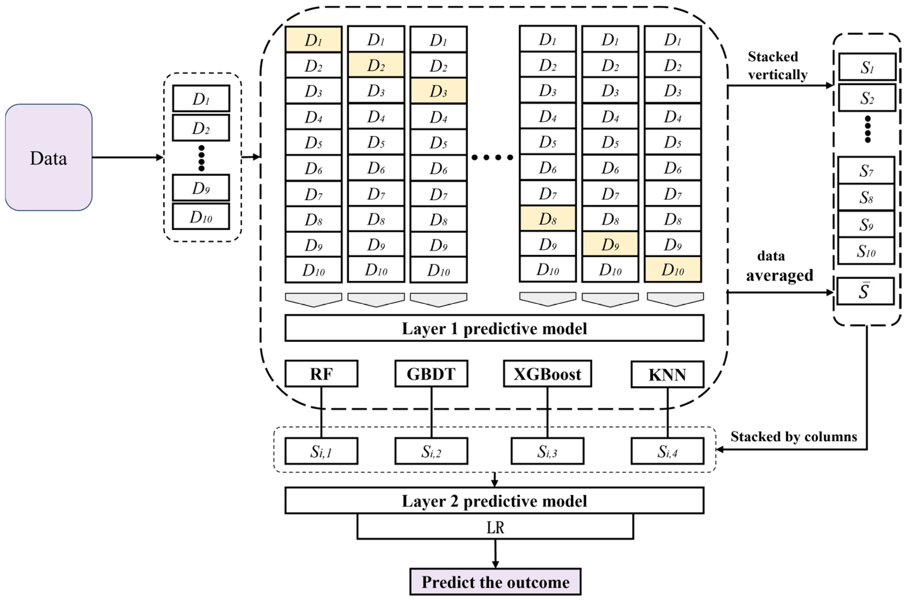
The 10-fold cross-validation method is employed to train each base learner. The original dataset D is divided into 10 mutually exclusive subsets, labeled D1 to D10. For each iteration, the union of 9 subsets is used as the training set, while the remaining subset serves as the test set. This process constructs the training and test sets for the primary learner, ensuring that each primary learner is trained and validated on 10 distinct sets of training and test data.

(3)

To construct a new training dataset for the Stacking ensemble model, the process involves leveraging the outputs of the four base learners. Each base learner is trained and tested using the same 10-fold cross-validation datasets. For the nth base learner, after completing the 10-fold cross-validation, 10 prediction results are generated. These results are vertically stacked by row to form the prediction set $S_{i,n}\left(i=1,2,\dots ,10\right)$, representing the sample data predictions under the base learner. Simultaneously, the 10 prediction results are averaged to produce ${\overline{S}}_n\left(n=1,2,\dots ,4\right)$, which serves as the input dataset $\left\{\left({\overline{S}}_n,S_{i,n}\right),i=1,2,\dots 10;n=1,2,\dots ,4\right\}$ for the second-layer meta-learner. This approach ensures that the meta-learner receives a comprehensive and refined input, enhancing the overall predictive performance of the Stacking ensemble model.

(4)

The meta-learner LR is used for secondary training, the new training set and test set generated by the base learner in the previous stage are inputted into the second-layer meta-learner for secondary training, and the final XCO₂ concentration prediction result is obtained.

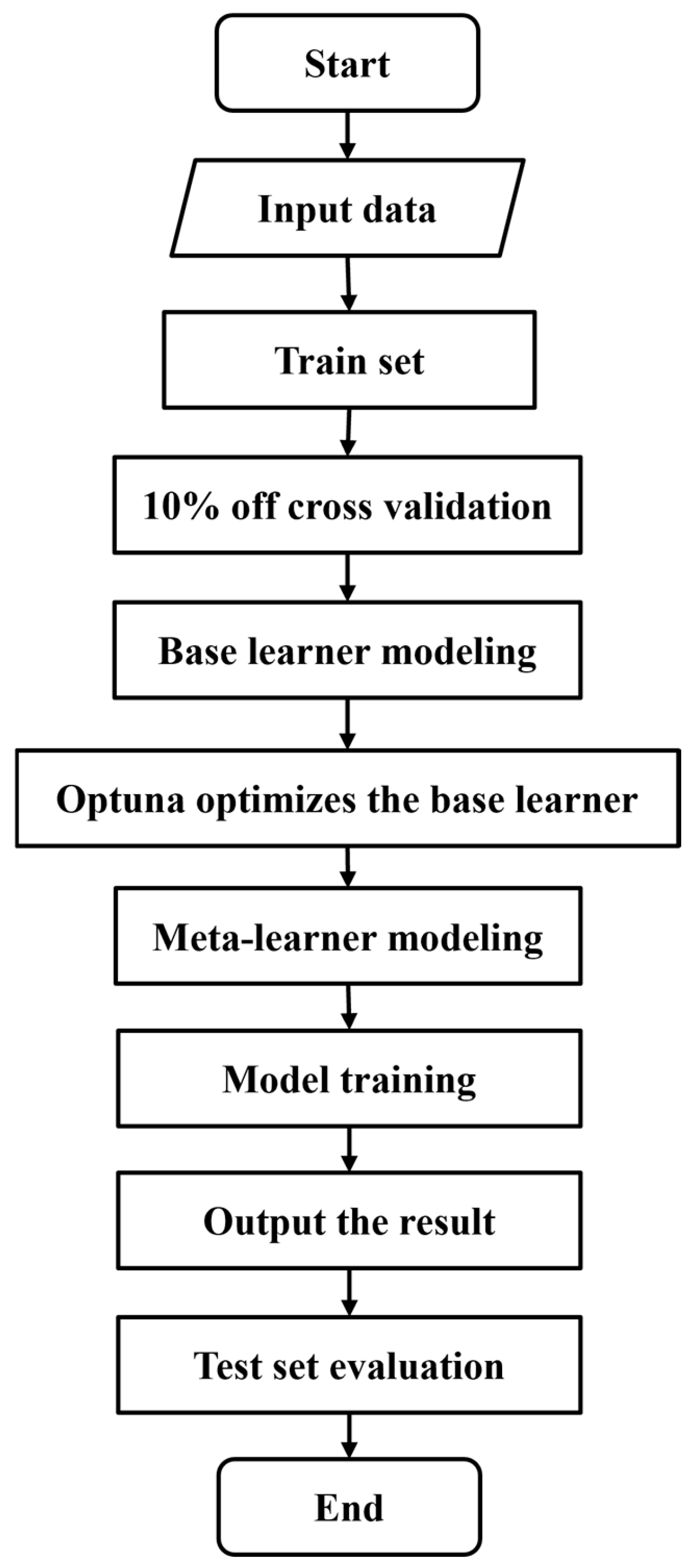
3.3. Optuna-Stacking Integrated Model

Optuna [27] employs the Tree-structured Parzen Estimator (TPE) algorithm, which combines the advantages of Bayesian optimization and the flexibility of decision trees to improve the efficiency of stacking model optimization. Optuna can effectively identify and terminate experiments with poor results, thereby saving computing resources and finding the optimal hyperparameter configuration within a limited number of iterations. Optuna’s parameter optimization process is as follows: First, the training set data are used for model training and hyperparameter optimization, and then cross-validation is performed on the training set. At the same time, the training set is used to train the base learner and adjust the hyperparameters, and the adjustment parameters, maximum number of iterations, and performance evaluation indicators of the RF, KNN, XGBOOST, and GBDT models are clarified; then, the next hyperparameter combination is selected through iteration for evaluation, and the experiments with poor results are pruned until the predetermined number of iterations is reached or the stopping condition is met; then, Optuna is used to optimize the hyperparameters and extract the best hyperparameter combination. The selected and trained base learner hyperparameter combination is further input into the meta-learner for training to construct the final prediction model. Finally, the performance of the model is evaluated using the test set to ensure its effectiveness and reliability. The process of the Optuna-Stacking integrated model is shown in Figure 6.

3.4. Model Evaluation Methods

To evaluate the accuracy of various models, a 10-fold cross-validation method was utilized. The dataset was randomly divided into 10 equal parts. In each iteration, 9 parts were used for training the model, while the remaining part was reserved for validation. This procedure was repeated 10 times, ensuring that each validation was conducted on an independent data subset. The coefficient of determination (R²), root mean square error (RMSE), and mean absolute error (MAE) between the model estimate and the satellite observation value are calculated as evaluation indicators. The value range of R² is 0 to 1. The higher the accuracy, the closer R² is to 1, and the smaller the MAE and RMSE are. MAE directly measures the average absolute difference between the predicted value and the true value, which can intuitively reflect the size of the error. RMSE is highly sensitive to outliers, and when there is noise in the data, RMSE can better identify it. This paper uses R², MAE, and RMSE to analyze and discuss the advantages and disadvantages of each model method and evaluate the model performance. The calculation formulas for each evaluation indicator are as follows:

$$\begin{array}{l}{R}^2=1-{\displaystyle \frac{{\displaystyle \sum _{i=1}^N{(y_i-{\widehat{y}}_i)}^2}}{{\displaystyle \sum _{i=1}^N{(y_i-{\overline{y}}_i)}^2}}}\\ RMSE=\sqrt{{\displaystyle \frac{1}{N}}{\displaystyle \sum _{i=1}^N{(y_i-{\widehat{y}}_i)}^2}}\\ MAE={\displaystyle \frac{1}{N}}\left|{\displaystyle \sum _{i=1}^N{(y_i-{\widehat{y}}_i)}^2}\right|\end{array}$$

(2)

In the formula, $y_i$ represents the XCO₂ satellite observation value; ${\overline{y}}_i$ represents the average value of the XCO₂ satellite observation; ${\widehat{y}}_i$ represents the XCO₂ estimated value; and N represents the total number of samples.

4. Results and Analysis

4.1. Hyperparameter Settings

To build a high-performing base learner, the Stacking ensemble learning model necessitates significant diversity among its base learners to ensure complementary effects. In this study, each base learner was initially trained and evaluated independently. The Optuna optimization framework, combined with 10-fold cross-validation, was employed to fine-tune the hyperparameters of each model, ensuring optimal performance within their respective domains. Upon completion of the optimization process, four base learners were constructed, with their hyperparameters meticulously tuned using the Optuna method. The specific parameter configurations are detailed in

Table 3. Hyperparameter settings of each model of base learner.

Model	Hyperparameters	Numeric
XGboost	max_depth	10
	learing_date	0.5
	n_estimators	116
	colsample_bytree	0.3
	subsample	0.5
KNN	k	3
RF	n_estimators	100
	max_depth	12
GBDT	n_estimators	178
	learning_rate	0.2
	max_depth	8

. The Optuna-optimized Stacking model significantly enhanced both the prediction accuracy and generalization capabilities, demonstrating the effectiveness of this approach in ensemble learning.

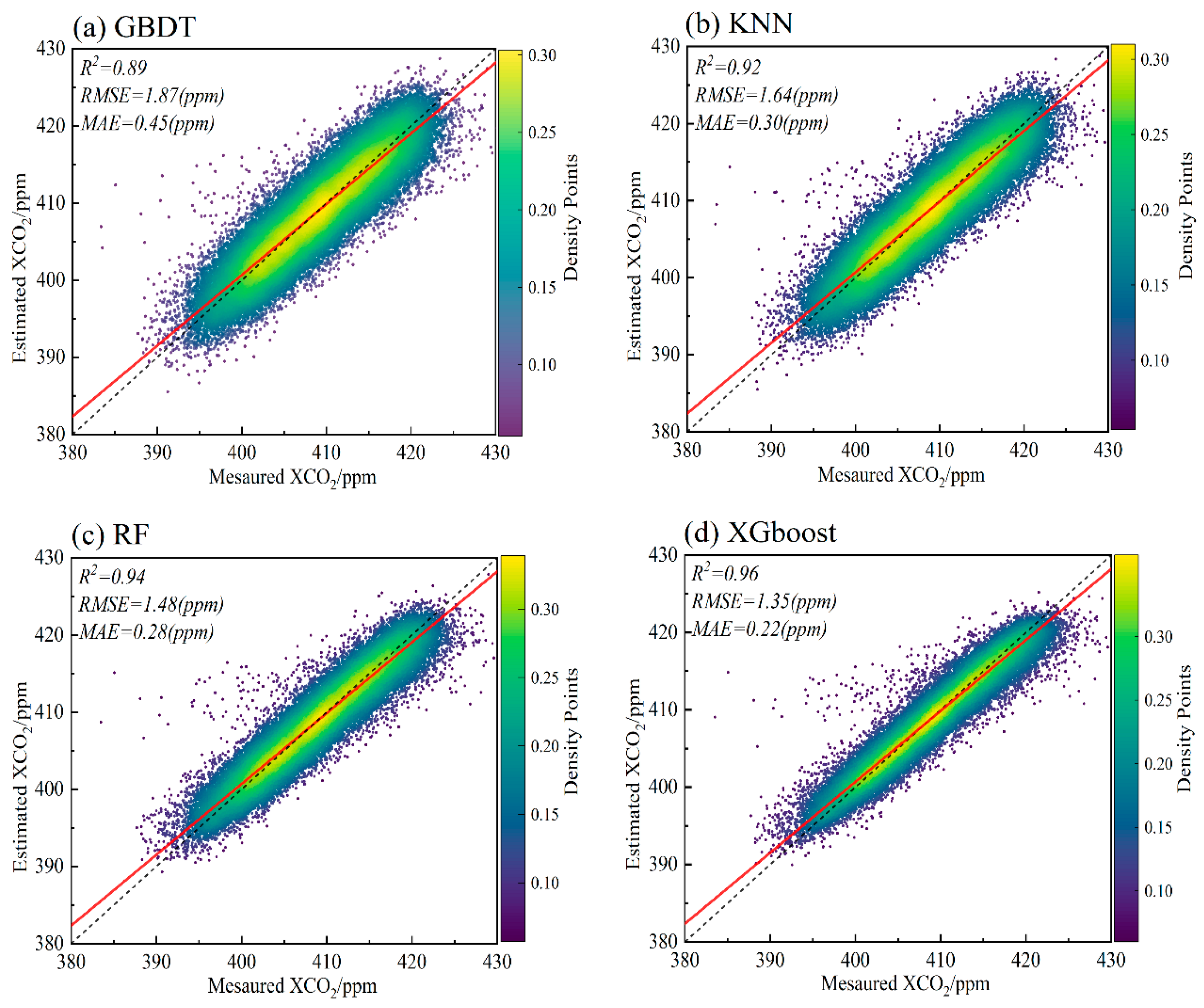
4.2. Model Cross-Validation Results

In order to comprehensively evaluate the generalization ability and robustness of the proposed model, this study used the cross-validation method to verify the model, and further compared and analyzed the Stacking model optimized by Optuna with four machine learning models: GBDT, KNN, RF, and XGBoost. The comparison structure of each model is shown in

Table 4. Comparison of model results.

Model	R2	RMSE	MAE
GBDT	0.890	1.87	0.45
KNN	0.922	1.64	0.30
RF	0.943	1.48	0.28
XGboost	0.964	1.35	0.22
Stacking	0.983	0.87	0.19

.

As shown in Table 4, the Stacking model performed best in all of the performance indicators, with an R² value of 0.983, which can explain 98.3% of the dependent variable variation. At the same time, the RMSE and MAE values of the Stacking model were 0.87 ppm and 0.19 ppm, respectively, which were significantly lower than those of the other four models. In contrast, although the XGBoost model had an R² value of 0.966, an RMSE of 1.35 ppm, and an MAE of 0.22 ppm, which performed well among single models, it was still lower than the Stacking model. The R², RMSE, and MAE of the GBDT model were 0.89, 1.87 ppm, and 0.45 ppm, respectively, and the performance was relatively low. This shows that a single model has limitations when dealing with complex nonlinear relationships, while the Stacking model can more effectively capture the nonlinear characteristics in the data and achieve a higher prediction accuracy by integrating the advantages of multiple algorithms, thereby effectively realizing the high-precision spatiotemporal distribution reconstruction of satellite XCO₂ data.

To further verify the effectiveness and limitations of each model in capturing the XCO₂ concentration change pattern, Figure 7 shows the scatter density diagram of the four models of GBDT, KNN, RF, and XGBoost when predicting the XCO₂ concentration. As can be seen from the figure, the scatter distribution of the XGBoost model is more concentrated, and the deviation from the diagonal line (ideal prediction line) is small, indicating that its prediction results are highly consistent with the actual observed values. In contrast, the scatter distribution of the GBDT model is more dispersed, especially in the high-concentration area, and the prediction deviation is large, indicating that it has certain deficiencies in dealing with complex nonlinear relationships. The prediction performance of the RF and KNN models is between that of XGBoost and GBDT, among which the prediction accuracy of the RF model in the high-concentration area is better than that of the KNN model, while the prediction performance of the KNN model in the low-concentration area is relatively good.

In addition, Figure 8 shows the accuracy comparison box plot and scatter plot of the Stacking model, which clearly reflects the advantage of the Stacking model in prediction accuracy. Its error distribution is more concentrated and has a smaller range, which further verifies its superiority in the task of high-precision spatiotemporal distribution reconstruction. This result shows that the Stacking model can effectively integrate the advantages of different models and overcome the shortcomings of a single model when processing satellite XCO₂ data, thereby achieving the efficient capture and high-precision prediction of complex nonlinear relationships.

Overall, the Stacking model can significantly improve the prediction accuracy by integrating the advantages of these single models, especially in terms of prediction consistency in high-concentration and low-concentration areas. This result further verifies the superiority and reliability of the Stacking model in the reconstruction of the spatiotemporal distribution of satellite XCO₂ data. Combined with the specific situation in Sichuan Province, the Stacking model can provide strong support for environmental monitoring and climate change research in the region, and help to more accurately estimate and analyze the changing trend in the XCO₂ concentration.

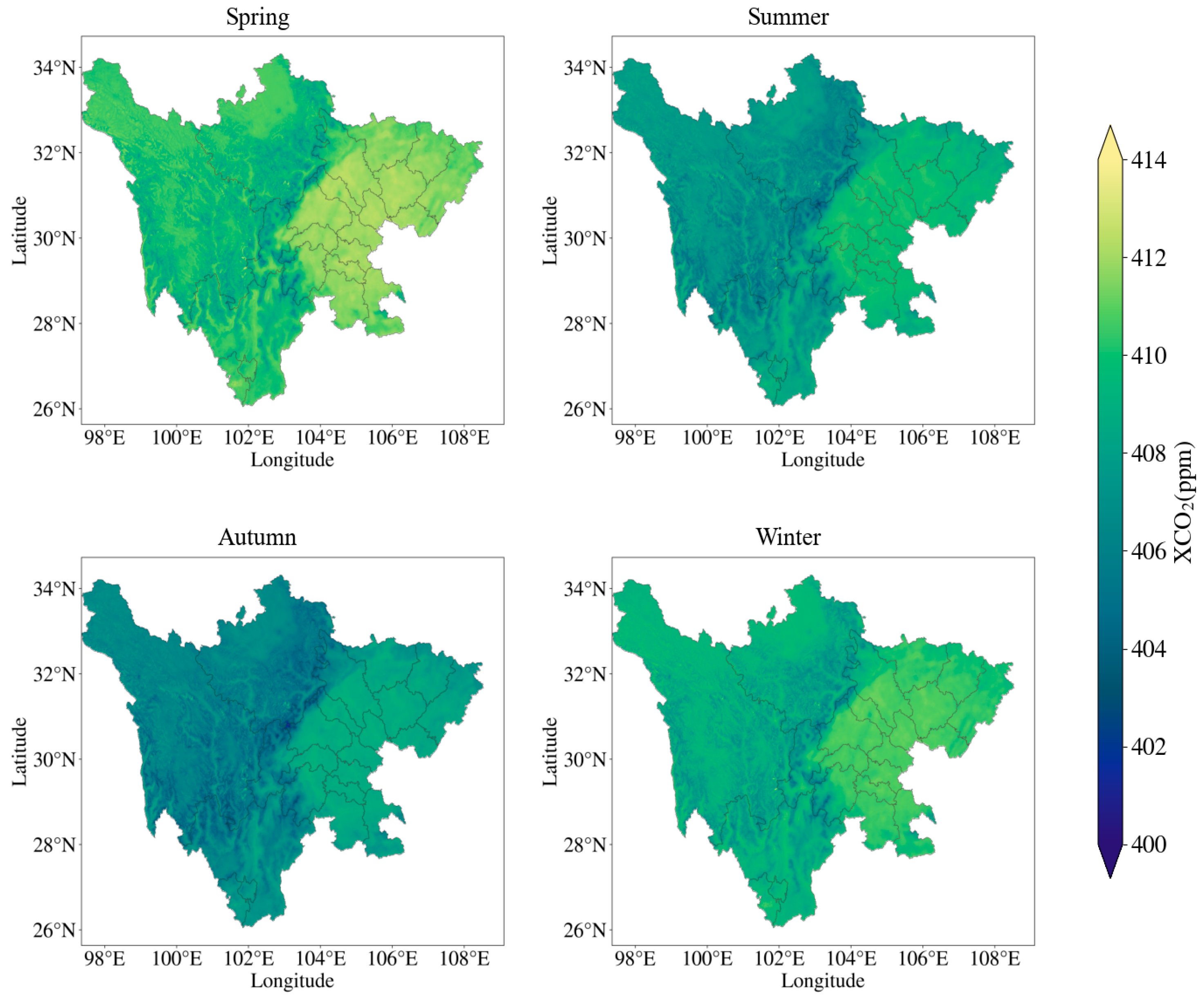
4.3. Stacking Seasonal Cross-Validation

To evaluate the temporal stability of the Stacking ensemble learning model, this study segmented the dataset spanning from 2015 to 2022 into four distinct seasons: spring (March–May), summer (June–August), autumn (September–November), and winter (December, January, and February). Each seasonal dataset was subjected to ten-fold cross-validation within the Stacking model. The seasonal statistical results are shown in

Table 5. Seasonal precision statistics.

Season	R2	RMSE	MAE
Spring	0.959	1.20	0.36
Summer	0.967	1.35	0.41
Autumn	0.980	0.95	0.22
Winter	0.976	1.13	0.39

, from which we can see the statistics and results of the evaluation indicators of the Stacking model’s four-season ten-fold cross-validation, demonstrating robust model performance across all seasons. Specifically, the model exhibited a comparable accuracy in autumn and winter, with R² values of 0.980 and 0.976, respectively. Furthermore, the mean absolute error (MAE) remained consistently below 0.2 ppm throughout the year, underscoring the reliability and precision of the Stacking model in estimating the regional XCO₂ concentrations in Sichuan Province. These findings highlight the model’s consistent performance across different seasons, as well as its capability to deliver high-precision XCO₂ concentration estimates. This demonstrates the Stacking model’s significant potential for applications in environmental monitoring and climate change research.

4.4. Stacking XCO₂ Dataset Verification with TCCON Sites

In order to accurately evaluate the accuracy of the model results, the measured data of the ground station (TCCON) were compared and analyzed with the model estimation results. Figure 9 shows the scatter plot of the TCCON station data and the Stacking XCO₂ dataset. It can be seen from the figure that the reconstructed XCO₂ dataset has a high overall consistency with the TCCON measured values. Although there are certain deviations, the deviation range is within a reasonable range. This result shows that the Stacking model can better capture the spatial distribution characteristics of XCO₂ and provide reliable data support for subsequent research. The XCO₂ concentrations at the two sites, Xianghe (XH) and Hefei (HF), showed an increasing trend over time. The XCO₂ concentrations at the XH and HF sites were highly correlated with the overall XCO₂ concentrations, with R² values of 0.96 and 0.98, and MAEs of 0.657 ppm and 0.639 ppm, respectively. This shows that the XCO₂ concentration trend at the two sites is consistent with that of Sichuan Province, and the error between the means is within ±1 ppm.

4.5. Temporal and Spatial Changes in Regional Carbon Concentration

Utilizing the Stacking model, this study constructed a high-resolution daily average XCO₂ concentration dataset for Sichuan Province from 2015 to 2022, with a spatial resolution of 1 km. This dataset provides detailed temporal and spatial insights into the XCO₂ distribution across the region. As illustrated in Figure 10, the multi-year average XCO₂ concentration in Sichuan Province exhibits a distinct east–west gradient, with higher concentrations in the east and lower concentrations in the west. This spatial pattern is closely linked to the province’s unique geographical features, characterized by a “mountainous crisscrossing and basin-embedded” landscape. Influenced by prominent mountain ranges such as Emei Mountain, Daba Mountain, and Min Mountain, and bounded by the Chengdu Plain, the Western Sichuan Plateau, and the Southern Sichuan hilly region, a “high-inside, low-around” carbon concentration distribution pattern emerges. Specifically, the eastern part of Sichuan, including cities such as Chengdu, Deyang, Nanchong, Yibin, and Luzhou, exhibits significantly higher XCO₂ concentrations compared to the western region. These areas form a “high-high” aggregation pattern of XCO₂ concentration, reflecting the combined effects of human activities, industrial development, and natural geographical constraints.

Overall, from 2015 to 2022, the XCO₂ levels in Sichuan Province have shown a steady increase, averaging 408.33 ppm annually. This increase is driven by the combined effects of geographical features, climatic conditions, and human activities. The spatial distribution of the XCO₂ concentrations has gradually stabilized, displaying distinct east–west differentiation and basin-centered agglomeration patterns. Specifically, the Sichuan Basin and its surrounding areas, characterized by rapid economic development and intensive human activities, have experienced substantial carbon emissions, leading to significantly higher XCO₂ concentrations. In contrast, the western and southern regions of Sichuan, marked by high altitudes, sparse population, low energy consumption, and extensive vegetation coverage, exhibit a pronounced carbon sink effect. Consequently, these areas demonstrate relatively lower XCO₂ concentrations and slower growth rates. This spatial heterogeneity underscores the interplay between natural factors and anthropogenic influences in shaping regional carbon dynamics, providing critical insights for targeted carbon management and climate mitigation strategies.

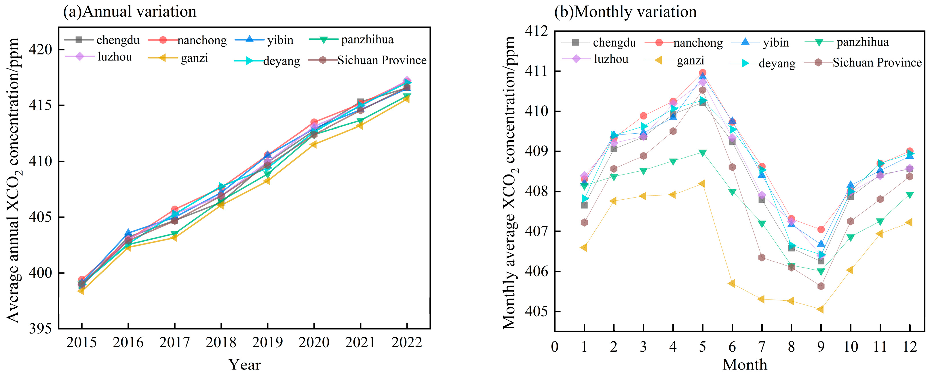
4.5.1. Temporal Characteristics of Atmospheric XCO₂ Concentration in Sichuan Province

The annual and monthly average XCO₂ concentrations of prefecture-level cities in Sichuan Province from 1 January 2015 to 31 December 2022 are shown in Figure 11. As shown in Figure 11, the average XCO₂ concentration in Sichuan Province has shown a significant upward trend. It was 398.9 ppm in 2015, which was at a relatively low level, and then increased year by year, rising to 416.6 ppm in 2022, with an average annual increase of 2.52 ppm. Notably, the rate of increase was higher from 2015 to 2019, averaging 2.66 ppm/year, but slowed to 2.12 ppm/year from 2020 to 2022. This deceleration may reflect the positive impact of emission reduction measures and environmental policies implemented in the region. Geographically, the distribution of XCO₂ concentrations revealed distinct regional variations. Cities such as Nanchong, Yibin, and Luzhou consistently exhibited high XCO₂ concentrations, forming persistent high-value zones. In contrast, the western and southwestern regions of Sichuan Province, including Ganzi Prefecture and Panzhihua City, demonstrated relatively lower XCO₂ levels. This spatial heterogeneity underscores the disparities in greenhouse gas emissions and atmospheric environmental quality across different regions of Sichuan Province. Although the atmospheric CO₂ concentration has continued to rise in recent years, the slowing growth rate highlights the ongoing challenges in addressing global climate change, advancing greenhouse gas emission reductions, and achieving carbon neutrality goals. These findings emphasize the need for sustained efforts in policy implementation and regional cooperation to mitigate carbon emissions and improve atmospheric quality.

In addition, the monthly average concentration of XCO₂ in Sichuan Province varies significantly, accumulating from September through the three seasons of autumn, winter, and spring until reaching the annual peak in May. This change pattern is closely related to the seasonal climate characteristics, vegetation growth cycle, and human activities in the region.

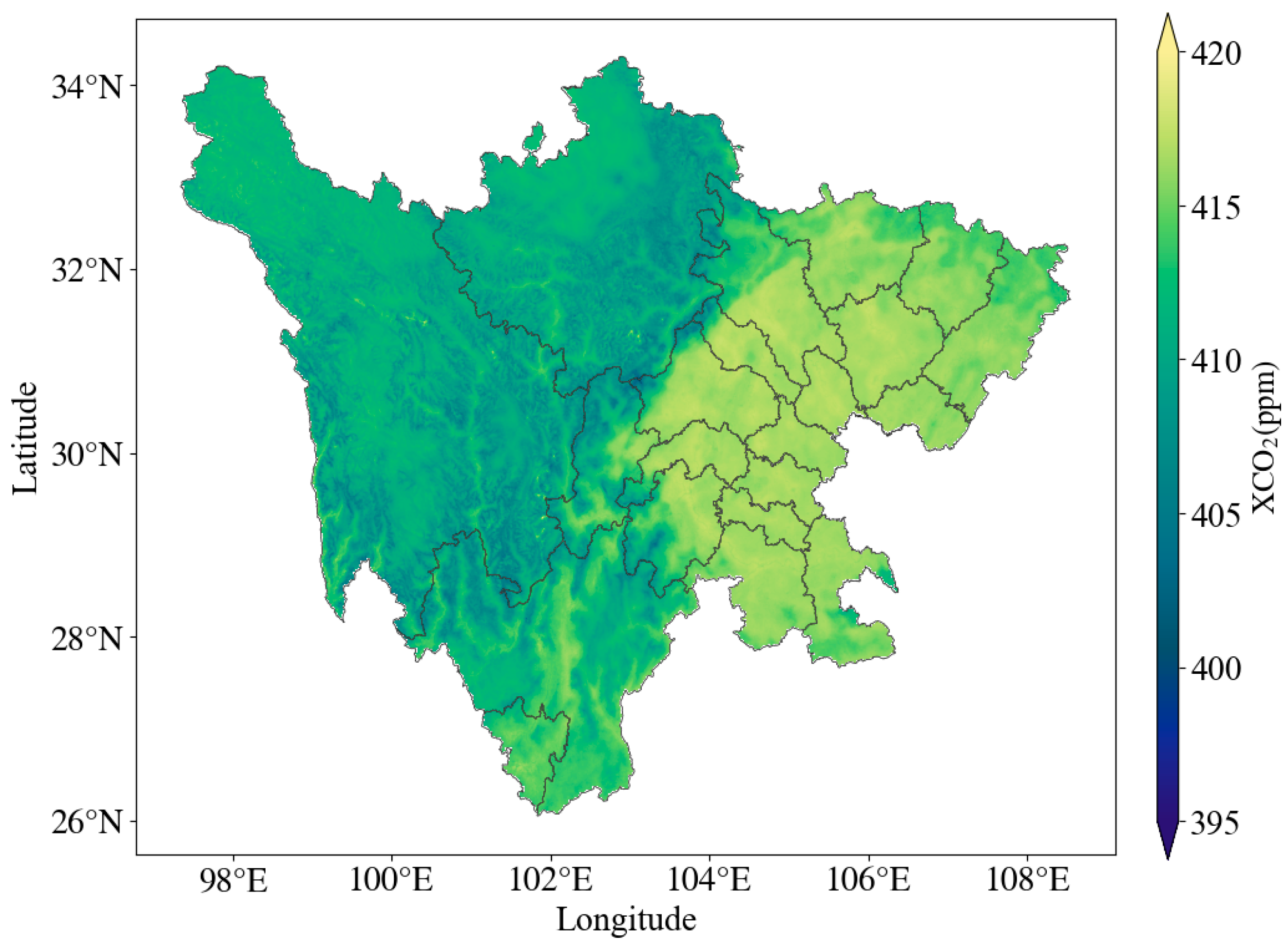
4.5.2. Spatial Distribution of Atmospheric XCO₂ Concentration in Sichuan Province

In order to accurately grasp the overall change in the XCO₂ concentration in Sichuan Province, the seasonal average concentration of XCO₂ in the region from 2015 to 2022 was estimated, and the statistical results are shown in

Table 6. Statistical results of XCO₂ concentration in spring, summer, autumn, and winter in Sichuan from 2015 to 2022.

Season	Maximum/ppm	Minimum/ppm	Average Value/ppm
Spring	425.235	397.646	410.190
Summer	427.332	393.351	408.731
Autumn	420.922	394.156	406.589
Winter	423.085	397.122	409.853

. The spatial distribution of the annual average seasonal concentration of XCO₂ in spring (March–May), summer (June–August), autumn (September–November), and winter (December–February of the following year) in Sichuan Province is shown in Figure 12. As can be seen from Figure 11, the seasonal change in the XCO₂ concentration in Sichuan Province is characterized by the seasonal periodic change in the XCO₂ concentration in the region, which is “high in winter and spring, low in summer and autumn”.

The main reasons for this are as follows: (1) In spring and winter, the change characteristics of the CO₂ concentration in the atmosphere are obvious. In winter, due to the drop in temperature, vegetation growth is restricted, carbon sink function is weakened, ecosystem respiration is inhibited, and photosynthesis efficiency is greatly reduced. At the same time, the high CO₂ emissions from human activities and biomass burning further promote the increase in atmospheric XCO₂ concentration. With the arrival of spring, as vegetation begins a new round of growth and development, photosynthesis gradually increases, but it still fails to surpass the respiration intensity of vegetation and soil, causing the CO₂ concentration in the atmosphere to reach its annual peak in spring. (2) In summer and autumn, vegetation enters a peak period of rapid growth and biomass accumulation. The intensity of photosynthesis increases significantly and exceeds the carbon emissions of vegetation and soil respiration, forming a significant carbon sink effect, resulting in a significantly lower CO₂ content in the atmosphere in summer and autumn than in spring and winter. Entering autumn, the high temperature and sufficient light conditions in summer further promote the peak performance of photosynthesis. The enhancement of photosynthesis and the improvement of the carbon sink capacity reduce the XCO₂ concentration to the lowest level throughout the year.

Specifically, from March to May, the temperature initially rebounded, the vegetation was in the early stage of growth, the vegetation and soil had strong respiration, and the continuous increase in CO₂ led to the high XCO₂ concentration in the whole area of Sichuan Province, ranging from 408.8 ppm to 410.5 ppm. From June to August, the high temperature, sufficient sunlight, and increased precipitation provided favorable conditions for plant growth. At this time, the photosynthesis of vegetation was greater than its own respiration and that of the soil, which caused the overall atmospheric XCO₂ in Sichuan Province to decline significantly, with the most obvious decline from June to July. From September to November, plant growth slowed down or stopped, photosynthesis weakened, microorganisms in the soil decomposed dead branches and leaves, resulting in enhanced respiration, and the carbon sink effect of vegetation decreased. The atmospheric XCO₂ in most parts of Sichuan began to rebound, rising to 407.8 ppm overall. In December, January, and February, the carbon sink capacity of vegetation was the weakest, and the photosynthesis of plants weakened, leading to an increase in the concentration of carbon dioxide in the atmosphere. At the same time, the temperature was low in winter, and the retention time of carbon dioxide in the atmosphere was longer, which increased the concentration of XCO₂ in winter to a higher level, then reaching its lowest level in January, reaching 407.2 ppm.

Overall, Sichuan Province shows significant dynamic changes in the carbon sink capacity of the ecosystem due to its significant differences in water and heat conditions, changes in light conditions, and zonal and vertical landform characteristics. The seasonal fluctuations in the concentration of XCO₂ in the region not only reflect the dynamic process of climate conditions and vegetation growth, but also provide an important basis for a deeper understanding of the regional carbon cycle mechanism.

5. Conclusions

This study combines the three forms of carbon satellite observation data of OCO-2, OCO-3, and GOSAT, meteorological data, NDVI data, land use type, population density, and other data, and uses the Stacking ensemble learning model optimized by Optuna. This model makes up for the limitations of a single model by integrating the advantages of multiple base learners, and effectively improves the prediction accuracy of XCO₂. Based on this, the spatiotemporal distribution dataset of the daily average concentration of XCO₂ in a 1 km grid in Sichuan Province from 2015 to 2022 was reconstructed, and its distribution and change trend in space and time were systematically analyzed. The analysis results reveal the spatiotemporal variation law of the atmospheric XCO₂ concentration in Sichuan Province, providing an important basis for understanding the characteristics of regional carbon emissions. The main contributions and conclusions are as follows:

(1)

In order to solve the problem of low spatial coverage and insufficient temporal resolution in the XCO₂ observation data of monitoring satellites, a high-coverage XCO₂ concentration inversion model integrating multi-source remote sensing data was proposed, and the accuracy of the Optuna-optimized Stacking ensemble learning model was comprehensively verified and evaluated, with the R² reaching 0.983, an RMSE of 0.87 ppm, and an MAE of 0.19 ppm. The results show that the Stacking XCO₂ dataset is significantly consistent with ground observation data, with the correlation coefficient between the model estimate and the observed value at the XH site being 0.96, and the correlation coefficient at the HF site being as high as 0.98. The model has shown a certain application potential in XCO₂ concentration monitoring and effectively reflects the long-term dynamic change characteristics of the atmospheric carbon dioxide concentration in Sichuan Province.

(2)

The atmospheric CO₂ concentration in Sichuan Province from 2015 to 2022 generally showed a fluctuating upward trend, from 398.9 ppm in 2015 to 416.6 ppm in 2022, but the growth rate has generally shown a downward trend in recent years. At the same time, the variation characteristics of the XCO₂ concentration on the annual, seasonal, and monthly scales were analyzed. In each year, the XCO₂ concentration showed the characteristics of being high in spring and winter and low in summer and autumn. Therefore, the atmospheric XCO₂ concentration in Sichuan Province has significant volatility and periodic characteristics.

(3)

The atmospheric CO₂ concentration in Sichuan Province shows obvious regional differences in spatial distribution, and the overall distribution pattern is “high in the east and low in the west”. Overall, the spatial distribution of the XCO₂ concentration is uneven, and the difference in extreme XCO₂ values between the different regions can reach 2.8 ppm, which is related to the local carbon source and carbon sink.

Given the heterogeneity of the regional development levels in Sichuan Province, as well as the complex interactions between geographical and climatic factors and human activities, the XCO₂ concentrations show significant differences in their temporal and spatial distribution. By deeply exploring the spatiotemporal variation characteristics of the atmospheric CO₂ concentration in Sichuan Province and the influencing factors behind it, we can reveal the geographical distribution, seasonal changes, and long-term trends in carbon emissions and absorption, and provide important support for low-carbon strategy formulation, adaptive planning, and carbon market risk assessment. Therefore, under the background of the “dual carbon” goal, it is urgent to actively promote the green transformation of the energy structure from the dual perspectives of carbon sources and carbon sinks, optimize the regional development pattern, optimize the regional development layout, enhance the natural and artificial carbon sink capacity, promote the innovation and application of low-carbon technologies, and strengthen environmental monitoring and the improvement of public environmental awareness to ensure effective response to climate change and promote the realization of sustainable development goals.

References

1. Bongaarts, J. IPCC, 2023: Climate Change 2023: Synthesis Report. IPCC, 184 p., doi: https://doi.org/10.59327/IPCC/AR6-9789291691647. Popul. Dev. Rev. 2024, 50, 577–580. [Google Scholar] [CrossRef]
2. Vandyck, T.; Keramidas, K.; Saveyn, B.; Kitous, A.; Vrontisi, Z. A global stocktake of the Paris pledges: Implications for energy systems and economy. Glob. Environ. Change 2016, 41, 46–63. [Google Scholar] [CrossRef]
3. Deng, S.; Shi, Y.; Jin, Y.; Wang, L. A GIS-based approach for quantifying and mapping carbon sink and stock values of forestecosystem: A case study. Energy Procedia 2011, 5, 1535–1545. [Google Scholar] [CrossRef]
4. Li, Z.; Xie, Y.; Shi, Y.; Li, Q.; COHEN, J.; Zhang, Y.; Han, Y.; Xiong, W.; Liu, Y. A review of collaborative remote sensing observation of greenhouse gases and aerosol with atmospheric environment satellites. Natl. Remote Sens. Bull. 2022, 26, 795–816. [Google Scholar] [CrossRef]
5. Gurney, K.R.; Liang, J.; O’keeffe, D.; Patarasuk, R.; Hutchins, M.; Huang, J.; Rao, P.; Song, Y. Comparison of global downscaled versus bottom-up fossil fuel CO2 emissions at the urban scale in four US urban areas. J. Geophys. Res. Atmos. 2019, 124, 2823–2840. [Google Scholar] [CrossRef]
6. Deng, F.; Jones, D.B.A.; O’Dell, C.W.; Nassar, R.; Parazoo, N.C. Combining GOSAT XCO2 observations over land and ocean to improve regional CO2 flux estimates. J. Geophys. Res. Atmos. 2016, 121, 1896–1913. [Google Scholar] [CrossRef]
7. Hu, K.; Liu, Z.; Shao, P.; Ma, K.; Xu, Y.; Wang, S.; Wang, Y.; Wang, H.; Di, L.; Xia, M.; et al. A review of satellite-based CO2 data reconstruction studies: Methodologies, challenges, and advances. Remote Sens. 2024, 16, 3818. [Google Scholar] [CrossRef]
8. Crisp, D.; Pollock, R.H.; Rosenberg, R.; Chapsky, L.; Lee, R.A.M.; Oyafuso, F.A.; Frankenberg, C.; O’Dell, C.W.; Bruegge, C.J.; Doran, G.B.; et al. The on-orbit performance of the Orbiting Carbon Observatory-2 (OCO-2) instrument and its radiometrically calibrated products. Atmos. Meas. Technol. 2017, 10, 59–81. [Google Scholar] [CrossRef]
9. Han, G.; Xu, H.; Gong, W.; Liu, J.; Du, J.; Ma, X.; Liang, A. Feasibility study on measuring atmospheric CO2 in urban areas using spaceborne CO2-IPDA LIDAR. Remote Sens. 2018, 10, 985. [Google Scholar] [CrossRef]
10. Liu, Y.; Wang, J.; Yao, L.; Chen, X.; Cai, Z.; Yang, D.; Yin, Z.; Gu, S.; Tian, L.; Lu, N.; et al. The TanSat mission: Preliminary global observations. Sci. Bull. 2018, 63, 1200–1207. [Google Scholar] [CrossRef]
11. Bhattacharjee, S.; Dill, K.; Chen, J. Forecasting Interannual Space-based CO2 Concentration using Geostatistical Mapping Approach. In Proceedings of the 2020 IEEE International Conference on Electronics, Computing and Communication Technologies (CONECCT), Bangalore, India, 2–4 July 2020; IEEE: Piscataway, NJ, USA, 2020; pp. 1–6. [Google Scholar]
12. Wang, W.; He, J.; Feng, H.; Jin, Z. High-Coverage Reconstruction of XCO2 Using Multisource Satellite Remote Sensing Data in Beijing–Tianjin–Hebei Region. Int. J. Environ. Res. Public Health 2022, 19, 10853. [Google Scholar] [CrossRef] [PubMed]
13. Chen, J.; Hu, R.; Chen, L.; Liao, Z.; Che, L.; Li, T. Multi-sensor integrated mapping of global XCO2 from 2015 to 2021 with a local random forest model. ISPRS J. Photogramm. Remote Sens. 2024, 208, 107–120. [Google Scholar] [CrossRef]
14. Duan, Z.; Yang, Y.; Wang, L.; Liu, C.; Fan, S.; Chen, C.; Tong, Y.; Lin, X.; Gao, Z. Temporal characteristics of carbon dioxide and ozone over a rural-cropland area in the Yangtze River Delta of eastern China. Sci. Total Environ. 2021, 757, 143750. [Google Scholar] [CrossRef]
15. Yang, Z.; Xu, Y.; Lu, X.; Mo, Y.; Ji, M.; Zhu, S. Spatialization of Atmospheric XCO2 in Xinjiang Uygur Autonomous Region based on OCO-2 Remote Sensing Data. Ecol. Environ. 2024, 33, 231. [Google Scholar]
16. Tang, Y.; Hu, J.; Tang, D.; Chen, Z. Spatio-temporal distribution of XCO2 concentrations in northeast China based on Downscaling-XGBoost model. In Proceedings of the International Conference on Remote Sensing, Mapping, and Geographic Information Systems (RSMG 2024), Zhengzhou, China, 19–21 July 2024; SPIE: Bellingham, WA, USA, 2024; Volume 13402, pp. 367–372. [Google Scholar]
17. Yao, Y.; Li, Z.; Wang, T.; Chen, A.; Wang, X.; Du, M.; Jia, G.; Li, Y.; Li, H.; Luo, W.; et al. A new estimation of China’s net ecosystem productivity based on eddy covariance measurements and a model tree ensemble approach. Agric. For. Meteorol. 2018, 253, 84–93. [Google Scholar] [CrossRef]
18. Eldering, A.; O’Dell, C.W.; Wennberg, P.O.; Crisp, D.; Gunson, M.R.; Viatte, C.; Avis, C.; Braverman, A.; Castano, R.; Chang, A.; et al. The Orbiting Carbon Observatory-2: First 18 months of science data products. Atmos. Meas. Technol. 2017, 10, 549–563. [Google Scholar] [CrossRef]
19. Eldering, A.; Wennberg, P.O.; Crisp, D.; Schimel, D.S.; Gunson, M.R.; Chatterjee, A.; Liu, J.; Schwandner, F.M.; Sun, Y.; O’dell, C.W.; et al. The Orbiting Carbon Observatory-2 early science investigations of regional carbon dioxide fluxes. Science 2017, 358, eaam5745. [Google Scholar] [CrossRef]
20. Yokota, T.; Yoshida, Y.; Eguchi, N.; Ota, Y.; Tanaka, T.; Watanabe, H.; Maksyutov, S. Global Concentrations of CO2 and CH4 Retrieved from GOSAT: First Preliminary Results. Sola 2009, 5, 160–163. [Google Scholar] [CrossRef]
21. Vogel, F.R.; Frey, M.; Staufer, J.; Hase, F.; Broquet, G.; Xueref-Remy, I.; Chevallier, F.; Ciais, P.; Sha, M.K.; Chelin, P.; et al. XCO2 in an emission hot-spot region: The COCCON Paris campaign 2015. Atmos. Chem. Phys. 2019, 19, 3271–3285. [Google Scholar] [CrossRef]
22. European Centre for Medium-Range Weather Forecasts. ERA5 Reanalysis [Data Set]. Copernicus Climate Change Service. 2018. Available online: https://cds.climate.copernicus.eu (accessed on 1 October 2023).
23. Reese, M. NASA Shuttle Radar Topography Mission (SRTM) Version 3.0 Global 1 Arc Second Data. NASA Earth Data, 1 March 2021. [Google Scholar]
24. Chen, J.P.; Zhang, C.X. Predicting Citation Counts of Papers. In Proceedings of the 2015 IEEE 14th International Conference on Cognitive Informatics & Cognitive Computing (ICCI*CC), Beijing, China, 6–8 July 2015; IEEE: Piscataway, NJ, USA, 2015; pp. 434–440. [Google Scholar]
25. Center for International Earth Science Information Network—CIESIN—Columbia University. Gridded Population of the World, Version 4 (GPWv4): Population Density, Revision 11; NASA Socioeconomic Data and Applications Center (SEDAC): Palisades, NY, USA, 2018.
26. Yue, L.Z.; Jian, H.C. Local Dependence Test Between Random Vectors Based on the Robust Conditional Spearman’s ρ and Kendall’s τ. Acta Math. Appl. Sin. Engl. Ser. 2023, 39, 491–510. [Google Scholar]
27. Akiba, T.; Sano, S.; Yanase, T.; Ohta, T.; Koyama, M. Optuna: A next-generation hyperparameter optimization framework. In Proceedings of the 25th ACM SIGKDD International Conference on Knowledge Discovery & Data Mining, Anchorage, AK, USA, 4–8 August 2019; pp. 2623–2631. [Google Scholar]
Figure 1. Overview of Sichuan Province.
Sustainability 17 03433 g001
Figure 2. Integrated OCO-2, OCO-3, and GOSAT satellite observation map for 2022.
Sustainability 17 03433 g002
Figure 3. Data preprocessing and model learning evaluation diagram.
Sustainability 17 03433 g003
Figure 4. Variable correlation heat map. 1. ELV, 2. POP, 3. TEM, 4. WIN_U, 5. WIN_V, 6. RELH, 7. BLH, 8. PRS, 9. LU, 10. NDVI, 11. XCO2.
Sustainability 17 03433 g004
Figure 5. Stacking training flow chart.
Sustainability 17 03433 g005
Figure 6. Optuna-Stacking integrated model flow chart.
Sustainability 17 03433 g006
Figure 7. Validation scatter plots of each model fit. The black dashed line represents the 1:1 line, and the red solid line represents the linear fitting result.
Sustainability 17 03433 g007
Figure 8. Stacking model box plot and validation scatter plot. The black dashed line represents the 1:1 line, and the red solid line represents the linear fitting result.
Sustainability 17 03433 g008
Figure 9. Comparison of Stacking XCO2 model results with TCCON monthly mean values.
Sustainability 17 03433 g009
Figure 10. Spatial distribution of average XCO2 concentration in Sichuan Province from 2015 to 2022.
Sustainability 17 03433 g010
Figure 11. Annual and monthly average XCO2 concentrations in prefecture-level cities in Sichuan Province from 2015 to 2022.
Sustainability 17 03433 g011
Figure 12. Spatial distribution of XCO2 concentration in Sichuan Province during the four seasons from 2015 to 2022.
Sustainability 17 03433 g012