Clustering-Based Urban Driving Cycle Generation: A Data-Driven Approach for Traffic Analysis and Sustainable Mobility Applications in Ecuador

Abstract

A representative urban driving cycle was developed for Quito, Ecuador, using the K-Means clustering method. From 64 samples and 188,713 geospatial and speed data points, a 2870 s driving cycle was constructed to capture real-world traffic characteristics. Key parameters include an average speed of 22.68 km/h, acceleration and deceleration rates of 0.55 m/s² and −0.57 m/s², and a dwell time of 9.66%. Due to Quito’s linear urban development, where mobility is limited to north–south/south–north corridors, the driving cycle reflects frequent accelerations and decelerations along congested arterial roads. A comparative analysis with international driving cycles revealed that Quito’s traffic follows a unique pattern shaped by its geographic constraints. The HK cycle in China showed the greatest similarities, although differences in instantaneous speeds highlight the need for localized models. While this study primarily focuses on methodological robustness, the developed driving cycle provides a foundational dataset for future research on traffic flow optimization, emissions estimation, and sustainable urban mobility strategies. These insights contribute to data-driven decision-making for improving transportation efficiency and environmental impact assessment in cities with similar urban structures.

1. Introduction

In recent decades, the accelerated population growth in developing countries has led to a significant increase in the number of vehicles, which negatively impacts the environment [1,2]. This phenomenon is particularly concerning in Latin America due to two main factors—the rapid urban development and the lack of adequate infrastructure to address the increase in vehicular traffic. Among the methods used to study the impact of vehicles on the environment is the analysis of driving cycles [3,4,5]. These cycles describe the behavior of a vehicle in terms of speed, acceleration, braking, and idling time. These parameters are fundamental for evaluating pollutant emissions, fuel consumption, and energy performance of vehicles under specific driving conditions [6].

Many consumer countries that do not produce vehicles use standardized or homologated driving cycles, such as the New European Driving Cycle (NEDC) and the Federal Test Procedure 75 (FTP-75) [6,7]. However, these cycles, designed for Europe and the United States, respectively, do not reflect the unique driving conditions of Latin American cities. This limits the accuracy of studies on pollution and fuel consumption, making it difficult to implement effective mitigation strategies.

In Latin America, some countries have begun to develop more representative driving cycles. For instance, in Chile, the NEDC cycle is used to estimate fuel consumption and emissions, although it is recognized that it does not fully reflect local conditions [8]. Brazil is in the process of creating its own cycles since the FTP-75 does not adequately match the driving profiles of its automotive fleet [9]. In Argentina, an analytical approach combines vehicle censuses and measurements on street segments to calculate emissions [10].

In Andean countries, cycles adapted to the region’s specificities have been designed. In Peru, the LMADC cycle was developed, showing significant differences from international standards [11]. Colombia has conducted studies in Pereira, located 1411 m above sea level, using low-cost methodologies. However, these cycles are not always applicable to other cities with different altitude and traffic conditions [12].

In Asia, countries like Singapore have designed their own driving cycles to reflect local conditions, allowing for more precise evaluations of fuel consumption and emissions [13]. In China, it has been noted that national cycles are not applicable to all regions, leading to the development of more representative local cycles. These initiatives highlight the need to consider geographical and demographic particularities when designing driving cycles [14].

Although some studies of driving cycles in Ecuador have been conducted, there are still no models that faithfully reflect the unique characteristics of its cities. Some studies, for example, use homologated cycles such as the NEDC to estimate emissions and the autonomy of electric vehicles [15]. However, these cycles, designed for European conditions, do not consider key aspects such as the mountainous topology, altitude, atmospheric conditions, cultural conditions, driving styles and mixed traffic typical of Andean cities (combination of public transport, buses, trolleybuses, private vehicles and motorcycles interacting on the same roads) [16]. This limits the accuracy of the studies and hinders the implementation of effective solutions to face the mobility challenges in our country.

In recent years, some researchers have begun to work in this area. For example, in Quito, urban, road and combined driving cycles were developed based on experimental data obtained with OBD devices. Although these studies offer an important first step, they were limited to a single vehicle and a small number of routes, and do not provide statistical sample size data for experimental development, which makes it difficult to generalize the results [17]. On the other hand, a specific cycle was designed for urban buses using weighted minimum differences (Azogues south of the capital of Ecuador). While this approach is valuable, it was not extended to other types of transport, nor did it consider the mixed traffic that characterizes larger cities [18].

Research in other cities (Cuenca) has explored how driving style affects energy consumption in electric vehicles. The use of machine learning allowed for the accurate modeling of battery state of charge, but the analysis was focused on a specific vehicle model (Kia Soul EV 2017), and did not consider the more complex dynamics of mixed traffic and multiple types of transportation [19,20]. For its part, in Loja, energy consumption was evaluated on routes with considerable slopes. However, this study was restricted to specific routes and did not consider more advanced technologies, such as the use of regenerative energy or hydrogen vehicles [21]. These works show an effort to adapt driving cycles locally, and expose their limitations, such as a reliance on small samples, restricted analysis to one type of vehicle, and a lack of comparison with international cycles, which calls for developing a more complex analysis approach that takes into account mixed traffic, complex topography and growing vehicle fleet.

The objective of this study is to develop a driving cycle adapted to the unique conditions of Quito, with emphasis on mixed traffic involving private vehicles and public transport buses. The motivation for this research arises from the need for a more accurate and representative urban driving cycle, considering (1) the dynamics of mixed traffic, (2) the impact of Quito’s complex topography, and (3) the influence of a growing vehicle fleet on urban mobility. Unlike previous studies, which were limited by small sample sizes, unique vehicle types, and a lack of international benchmarks, this work addresses these limitations by integrating a diverse dataset [17,18,19,20,21].

The main contributions of this study include the development of a data-driven urban driving cycle specifically tailored to Quito’s conditions, the incorporation of multiple vehicle types to improve statistical robustness, the application of K-means clustering and Markov models to construct a cycle that reflects actual driving patterns, and an international comparative analysis with ten globally recognized driving cycles from the Americas, Europe and Asia, thus ensuring that the results are relevant beyond the local context. Using 64 road test samples covering five different vehicle types and 188,713 speed and geospatial data points, a statistically robust representation of Quito’s driving conditions is ensured.

K-means has certain well-known limitations, such as sensitivity to centroid initialization, the need to predefine $\mathrm{k}$, the assumption of spherical clusters and the possibility of converging to local optima. To mitigate these problems, multiple runs of the algorithm need to be performed, and consequently the solution with the lowest Sum of Squared Errors (SSE) should be selected to improve the stability of the clusters [22]. Additionally, the elbow method is used to determine the optimal number of clusters, avoiding the loss of information due to under-segmentation and the formation of non-representative clusters due to over-segmentation. Although K-Means++ is another alternative with improved centroid initialization, its application in driving cycle segmentation remains less explored compared to standard K-means [23]. Since previous studies have successfully applied standard K-means to microstrip segmentation and drive cycle characterization, it is considered a valid and effective choice for this study [24,25,26].

This work contains four sections. The first introduces the context and relevance of the study; the second describes the methodology for data acquisition and processing, with emphasis on the use of the k-means algorithm; the third one presents the results obtained together with the comparison of the cycle developed with recognized international cycles; and finally, the fourth chapter summarizes the findings of the study and raises future perspectives to continue with this line of research.

2. Methodology

A structured methodology is used, which will help to develop the driving cycle adapted to the specific conditions of high-altitude cities such as Quito, Ecuador. As shown in Figure 1, the methodology is divided into two stages; the first one is focused on the acquisition of experimental data on the driving speed in real time, and the second one is the data processing for the generation of the cycle.

2.1. Acquisition of Experimental Data

2.1.1. Route Selection

In this study, a route of approximately 18.24 km has been defined within the city of Quito, located at an altitude of 2850 m above sea level. The selected route covers the south, center and north of the city, connecting point A (Instituto Mayor Pedro Traversari, in the south) with point B (Parque Inglés, in the north). Mariscal Sucre Avenue is the main axis linking these two points; see Figure 2.

The selection of this 18.24 km route was based on statistical and urban planning considerations to ensure that it represents a wide range of driving conditions in Quito [25]. Studies of urban mobility patterns in the city indicate that most daily trips range between 15 km and 20 km, so this is a representative length of an urban driving cycle. This route has the highest levels of congestion within the metropolitan district of Quito, especially during peak hours (6:00 to 9:30 and 18:00 to 21:00), when most traffic flows from the south of the city to the work and study areas in the center and north [27,28].

One of the main innovations of this study is its ability to capture actual driving conditions in Quito’s mountainous terrain and high-altitude environment. Unlike traditional urban driving cycle models, which assume uniform road conditions, this study integrates data from roads with varying inclines and altitudes, resulting in a more realistic representation of vehicle performance and energy consumption. In addition, the study explicitly accounts for mixed traffic scenarios, including interactions between private vehicles and public transport, a factor not included in previous research.

2.1.2. Sample Size

Previous studies on urban driving cycles in Ecuador have been based on limited sample sizes. To ensure statistical robustness, a sample size is determined based on a 95% confidence level and a 5% margin of error. The final data set obtained consists of 64 experimental trials, covering different traffic conditions and vehicle types, improving the accuracy and representativeness of the cycle generated.

Equation (1) is used to calculate the sample size $\mathrm{n}$, considering a confidence level of 95% and an assumed margin of error ($\mathrm{E}$) of 5%. The standard deviation ($\mathsf{\sigma }$) is initially estimated from 35 pilot tests, using Equation (2). Substituting the obtained value of the standard deviation in Equation (1), the representative sample size is determined to be 64 tests [29,30]. These tests are conducted on the main avenue Mariscal Sucre during peak hours, specifically from 6:00 a.m. to 9:30 a.m. and from 6:00 p.m. to 9:00 p.m., to capture the highest vehicular traffic conditions.

$$\mathrm{n}={\displaystyle \frac{{\mathrm{z}}^2·{\mathsf{\sigma }}^2}{{\mathrm{E}}^2}},$$

(1)

where $z$ is the critical value (confidence level 95%).

$$\mathsf{\sigma }=\sqrt{{\displaystyle \frac{{\sum }_{\mathrm{i}=1}^{\mathrm{n}}{({\mathrm{x}}_{\mathrm{i}}-\stackrel{\mathrm{-}}{\mathrm{x}})}^2}{\mathrm{n}-1}}},$$

(2)

where ${\mathrm{x}}_{\mathrm{i}}$ is the individual value in the sample, $\stackrel{\mathrm{-}}{\mathrm{x}}$ is the arithmetic mean of the sample, and $\mathrm{n}-1$ is the degrees of freedom, to correct for the estimation bias of the sample’s variability.

2.1.3. Data Collection

The collection of experimental speed data and geospatial information, such as latitude, longitude and heading, was performed using a mobile application called MATLAB Mobile version 6.7.0, developed by MathWorks [31].

Table 1. Devices and vehicles used for GPS data collection.

ID	Vehicle Make and Model	Vehicle Technical Specifications	GPS Device (Smartphone)	Phone Technical Specifications	GPS Sampling	Additional Comments
1	Sedan JAC-S3 2019	1.6 L engine, gasoline, manual transmission	Redmi Note 9	MediaTek Helio G85 octa-core 2 GHz, Mali-G52 MC2, Android 10, Dual-Band GPS	2 Hz	Dense traffic route, nighttime conditions
2	Pickup Truck Mitsubishi L200 2009	2.5 L engine, diesel, 4 × 4 drive	Redmi Note 12	Snapdragon 4 Gen 1, 2 GHz, 128 GB, Android 10, Dual-Band GPS	2 Hz	Dense traffic route, nighttime conditions
3	Hatchback Chevrolet Aveo 2010	1.5 L engine, gasoline, manual transmission	Huawei Y9	Kirin 710, Octa-core, 12 nm, Mali-G51 MP4 GPU	2 Hz	Dense traffic route, nighttime conditions
4	Pickup Truck Mazda BT50 2019	3.0 L engine, diesel, rear-wheel drive, manual transmission	Huawei Mate 40 Pro	Kirin 9000, 8 GB RAM, Android 11, Dual-Frequency GPS	1 Hz	Dense traffic route, nighttime conditions
5	Hatchback Corza Wind 2002	1.4 L engine, gasoline, manual transmission	OnePlus 11	Snapdragon 8 Gen 2, 16 GB RAM, Android 13, Multi-Frequency GNSS	2 Hz	Dense traffic route, nighttime conditions

shows the devices used in this data collection phase, which included five smartphones that acted as GPS sensors during the selected route. The information was sent in real time and stored in the cloud for further processing. The phones were installed in a total of five vehicles of different brands and characteristics. Importantly, to mitigate deviations in GPS position, cell phones with high-end processors were used, and a stable satellite connection was ensured throughout the route. However, it should be noted that this measure does not take into account the effects of the uncertainties inherent in the measurement of the devices, which could introduce slight variations in the data collected [32,33,34]. The selection of vehicles and smartphones was designed to ensure a representative and high-quality dataset for the generation of driving cycles. The vehicles used in this study cover the various urban mobility scenarios, including compact cars, sedans and larger diesel vans, which are commonly used in Quito’s mixed traffic. This selection attempts to minimize the bias of using a single vehicle type, ensuring that the driving cycle developed reflects driving conditions in a real environment.

As for the smartphones used for data collection, devices with dual or multi-frequency GPS were used to ensure high positioning accuracy, reducing possible errors due to the effects of urban canyons. In addition, smartphones with high-end processors were used to allow real-time data transmission with constant sampling rates of 1–2 Hz.

2.2. Data Processing

2.2.1. Extraction of Microtrips

The collected experimental velocity and geospatial parameter data were segmented into micro-strips for ease of manipulation and analysis. This allowed the experimental data to be approached using algorithms designed for statistical analysis, clustering and predictive modeling. Microtrips allow for segmenting an entire driving cycle into smaller, homogeneous and analytically manageable units. Such segmentation offers the great advantage of providing greater precision in the identification of specific driving patterns, representing in a more detailed way the vehicle dynamics [35,36,37].

To perform the extraction, Equation (3) was used, in which the $\mathrm{X}$ data set is organized in the form of a matrix wherein each row represents a microtrip and each column a feature associated with it. Each microtrip is defined as a continuous driving interval characterized by specific attributes, such as average speed (${\mathrm{v}}_{\mathrm{i}}$), duration (${\mathrm{t}}_{\mathrm{i}}$), average acceleration (${\mathrm{a}}_{\mathrm{i}}$) and average deceleration (${\mathrm{d}}_{\mathrm{i}}$). This segmentation allows for the elimination of prolonged periods of detention and irrelevant events, ensuring that the analyzed data represent the actual driving conditions on the studied route.

$$\mathrm{X}=\left[\begin{array}{cccc}{\mathrm{v}}_1& {\mathrm{t}}_1& {\mathrm{a}}_1& {\mathrm{d}}_1\\ {\mathrm{v}}_2& {\mathrm{t}}_2& {\mathrm{a}}_2& {\mathrm{d}}_2\\ ⋮& ⋮& ⋮& ⋮\\ {\mathrm{v}}_{\mathrm{n}}& {\mathrm{t}}_{\mathrm{n}}& {\mathrm{a}}_{\mathrm{n}}& {\mathrm{d}}_{\mathrm{n}}\end{array}\right].$$

(3)

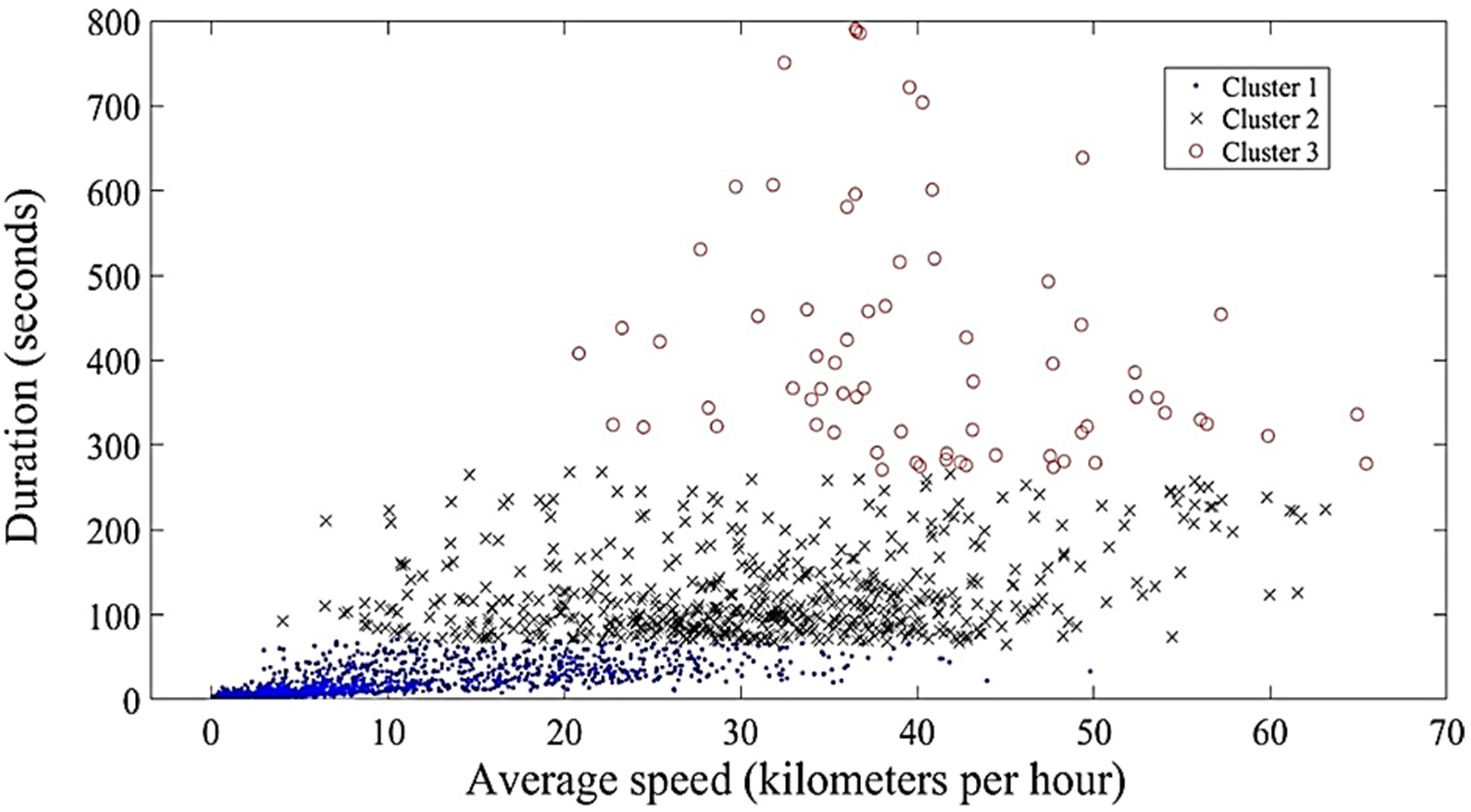
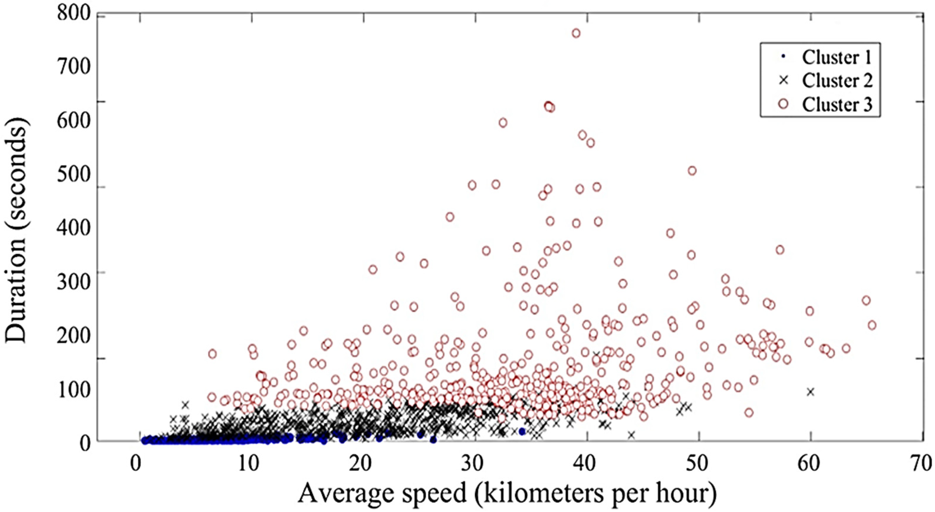
2.2.2. K-Means Clustering Method for Driving Cycle Construction

The k-means method for the construction of driving cycles is widely used. This unsupervised machine learning algorithm is used to segment a data set by grouping similar vehicle dynamics patterns into a predefined number of groups or clusters ($\mathrm{k}$). One of its main advantages is the ability to minimize the dispersion within clusters while maximizing the separation between them, iteratively refining the centroids until convergence is achieved [33,34,35]. Equation (4) is used for cluster formation, assigning each data point to the cluster whose centroid is closest. In this case, Alpha-Beta divergence is used as a metric to calculate the quadratic distance of each $\mathrm{X}$ data point [38,39].

$$\underset{\mathrm{j}}{\min }{\mathrm{d}}^2\left({\mathrm{x}}_{\mathrm{i}},{ \mathrm{c}}_{\mathrm{j}}\right),$$

(4)

where $\mathrm{d}$ is the selected distance measure (Alpha–Beta divergence), ${\mathrm{x}}_{\mathrm{i}}$ is the data point ($\mathrm{i}=1, \dots , {\mathrm{n}}_{\mathrm{j}}$), and ${\mathrm{c}}_{\mathrm{j}}$ is the centroid of cluster j $(\mathrm{j}=1, \dots , \mathrm{k})$.

Cluster centroids are updated using Equation (5). The centroids of each cluster are recalculated considering only the data assigned to that cluster. This step ensures the minimization of the distortion error. This process iteratively reassigns and recalculates the clusters and centroids, respectively, until convergence is reached [38].

$$\mathrm{e}\left({\mathrm{x}}_{\mathrm{j}}\right)=\sum _{\mathrm{i}=1}^{{\mathrm{n}}_{\mathrm{j}}}{\mathrm{d}}^2\left({\mathrm{x}}_{\mathrm{i}},{\mathrm{c}}_{\mathrm{j}}\right).$$

(5)

The convergence criteria are a fundamental parameter, evaluated by Equation (6). The developed program ends when a stable assignment of data points to the clusters is achieved or, failing that, when a maximum number of iterations is reached [38,40].

$$\mathrm{e}\left(\mathrm{X}\right)=\sum _{\mathrm{j}=1}^{\mathrm{k}}\sum _{\mathrm{i}=1}^{{\mathrm{n}}_{\mathrm{j}}}{\mathrm{d}}^2\left({\mathrm{x}}_{\mathrm{i}},{\mathrm{c}}_{\mathrm{j}}\right).$$

(6)

2.2.3. Elbow Method for Determining K, the Optimal Number of Clusters

To determine the optimal number of clusters ($\mathrm{k}$) in the development of the driving cycle, the elbow method was used; see Equation (7). This method evaluates the sum of ($\mathrm{SSE}$) within clusters as k increases. The SSE is calculated as the quadratic distance between the data points and their respective centroids, which decreases rapidly until an inflection point (elbow) is reached. This point marks the optimal value of k, because thereafter the reduction in SSE can be considered depreciable [41,42].

$$\mathrm{SSE}=\sum _{\mathrm{i}=1}^{\mathrm{k}}\sum _{\mathrm{x}\in {\mathrm{C}}_{\mathrm{i}}}{‖\mathrm{x}-{\mathrm{u}}_{\mathrm{i}}‖}^2,$$

(7)

where $\mathrm{k}$ is the number of clusters, ${\mathrm{C}}_{\mathrm{i}}$ is a set of points in cluster $\mathrm{i}$, ${\mathrm{u}}_{\mathrm{i}}$ is the centroid of cluster i, and ${\Vert \mathrm{x}-{\mathrm{u}}_{\mathrm{i}} \Vert }^2$ is the quadratic distance between a point x and its centroid.

2.3. Construction of Driving Cycles with Microtrips

For the construction of the driving cycle using microtrips, two phases are followed. In the first, an initial micro-trip is used to start the cycle. Subsequently, a second micro-trip is selected using a simple Markov chain model, repeating this process iteratively. To model the Markov chain, a transition matrix is required that calculates the probability of transition from one specific group to another. The probabilities are accumulated by row, and a value of 1 is selected [25,43]. Depending on the column interval in which this value falls within a specific row, the next group is determined. This procedure continues until the total required length for the candidate cycle is reached.

Equations (8) and (9) are used to calculate the average error of the candidate cycle.

$${\mathrm{S}}_{\mathrm{i}}=\left({\displaystyle \frac{\left|{\mathrm{p}}_{\mathrm{i}}-{\mathrm{P}}_{\mathrm{i}}\right|}{{\mathrm{P}}_{\mathrm{i}}}}\right),$$

(8)

where ${\mathrm{P}}_{\mathrm{i}}$ is the target parameter i of all the data collected, and ${\mathrm{p}}_{\mathrm{i}}$ is the target parameter i of the candidate cycle.

The mean error is calculated by the equation

$$\mathrm{ME}={\displaystyle \frac{ \sum _{\mathrm{j}=1}^{\mathrm{n}}{\mathrm{S}}_{\mathrm{i}}}{\mathrm{n}}},$$

(9)

where n is the number of evaluation parameters and ${\mathrm{S}}_{\mathrm{i}}$ is the relative error of the $\mathrm{i}-\mathrm{th}$ parameter.

This work presents the parameters selected to establish the criteria for characterizing the representative driving cycles, which are detailed in

Table 2. Analysis criteria and characteristic kinematic parameters.

Criteria	Abbreviation	Unit
Distance	D	$\mathrm{km}$
Cycle time	T	$\mathrm{s}$
Average speed for entire trip	V	$\mathrm{km}·{\mathrm{h}}^{-1}$
Average running speed	Vr	$\mathrm{km}·{\mathrm{h}}^{-1}$
Standard deviation of speed	V sd	$\mathrm{km}·{\mathrm{h}}^{-1}$
Standard deviation of acceleration	A sd	$\mathrm{m}·{\mathrm{s}}^{-2}$
Average acceleration of all acceleration phases	aa	$\mathrm{m}·{\mathrm{s}}^{-2}$
Average deceleration of all acceleration phases	ad	$\mathrm{m}·{\mathrm{s}}^{-2}$
Root mean square acceleration	arms	$\mathrm{m}·{\mathrm{s}}^{-2}$
Positive acceleration kinetic energy	PKE	$\mathrm{m}·{\mathrm{s}}^{-2}$
Percentage of idle time (speed = 0)	Pi	%
Percentage of time spent in acceleration mode (a > 0.1 m·s−2)	Pa	%
Percentage of time spent in deceleration mode (d < −0.1 m·s−2)	Pd	%
Percentage of time spent in cruise mode (Pc) (−0.1 m/s2 < acceleration < 0.1 m/s2, speed > 5 kmph)	Pc	%

[44].

3. Results

Figure 3 shows the number of clusters versus the sum of SSE or inertia, which measures the distance between the data points and the centroid of their respective clusters. In the plot, one can identify the inflection point, or the “bend”, in the curve, where the reduction in squared error begins to decrease significantly. This plot suggests that the optimal number of clusters needed to construct the driving cycle is 3.

A total of 188,713 experimental data have been plotted in Figure 4, where the distribution of the clusters obtained by the k-means algorithm, described in Section 2.2.2, is shown. The data are organized into three clusters, classified according to two characteristics, average speed and duration. Each cluster is distinguished by a different color and symbol.

So-called cluster 1 (blue dots) contains paths with low average speed and short duration, concentrating in a range of values from 0 to 10 km/h in a time of up to 100 s. Cluster 2 (black curves) includes paths with moderate average speeds; there is greater variability in duration here, with a range of speeds between 10 and 40 km/h. Cluster 3 (red circles) represents paths with higher average speeds, which exceed 30 km/h and, for the most part, have durations greater than 300 s.

A complementary analysis was performed to compare K-means with Gaussian mixture models (GMM), as shown in Figure 5. Although GMM is advantageous for modeling continuous transitions between clusters, the results indicate that it introduces probabilistic ambiguities, making it difficult to classify moderate traffic and free-flow conditions. In addition, GMM showed high sensitivity to outliers, which affected covariance estimation and cluster assignment stability [45]. Therefore, K-means is chosen as the main clustering method, as it provides well-defined clustering boundaries and ensures a clear segmentation of driving conditions needed to construct a representative urban driving cycle in Quito.

Table 3. Transition matrix of clusters used for modeling.

Initial Cluster	Rear Cluster 1	Rear Cluster 2	Rear Cluster 3
1	0.7933	0.188	0.0209
2	0.5300	0.4408	0.0292
3	0.4746	0.4407	0.0847

presents the transition matrix used in the Markov chain model, which determines the probability of moving from one driving state to another. The three groups represent different driving conditions: (1) low speed and short duration (high congestion), (2) moderate speed and variable duration (constant driving), and (3) high speed and long duration (free-flow conditions). Each row of the table shows the probability that a vehicle will remain in the same group or switch to another. The transition probabilities, for example, indicate that vehicles in group 1 (stop-and-go traffic) have a high probability (79.33%) of remaining in congestion, while those in group 3 (high-speed driving) tend to move to lower speeds (47.46% probability of moving to group 2). These probabilities play a key role in shaping the final driving cycle, ensuring that it accurately reflects the actual traffic dynamics in Quito.

Figure 6 shows the average error of the candidate cycles, measured as a percentage, and the duration of the driving cycle, expressed in seconds. This analysis is performed over a range from 600 to 3400 s, increasing in steps of 200 s. It can be observed that, as the cycle length increases, the average error tends to decrease, indicating that longer cycles offer a more robust statistical representation, and some points where the curve shows fluctuations can also be appreciated, indicating variations in the accuracy according to the cycle length. In this work, it is estimated that the most favorable point is around 2800 s, where the average error reaches its minimum at 5.00%. However, when exceeding this duration, the error shows a slight tendency to increase, suggesting that longer cycles could include elements that do not contribute much to the accuracy. This highlights the duration of 2800 s as an ideal balance point between representativeness and cycle complexity.

The objective parameters used for the comparative evaluation of the candidate driving cycles, based on the experimental values obtained on the test routes, are presented in

Table 4. Objective parameters for driving cycle evaluation.

Parameter	Value	Parameter	Value
V (km/h)	23.21	${\mathrm{P}}_{\mathrm{i}}$ (%)	24.07
Vr (km/h)	30.03	${\mathrm{P}}_{\mathrm{c}}$ (%)	13.79
A $(\mathrm{m}/{\mathrm{s}}^2)$	0.55	${\mathrm{P}}_{\mathrm{cr}}$ (%)	23.55
ad $(\mathrm{m}/{\mathrm{s}}^2)$	−0.57	${\mathrm{P}}_{\mathrm{ad}}$ (%)	23.50
${\mathrm{P}}_{\mathrm{a}}$ (%)	36.97	${\mathrm{a}}_{\mathrm{rms}} (\mathrm{m}/{\mathrm{s}}^2)$	0.63
${\mathrm{P}}_{\mathrm{d}}$ (%)	35.02	PKE $(\mathrm{m}/{\mathrm{s}}^2)$	0.20

. It is observed that the average speed (V) is 23.21 km/h, while the representative speed (Vr) is 30.03 km/h. The average acceleration (A) and average deceleration (ad) values are 0.55 m/s² and −0.57 m/s², respectively. In addition, percentage values are included that evaluate aspects such as power in acceleration (Pa), deceleration (Pd) and inactive moments (Pi). These parameters allow a detailed analysis of the behavior of the candidate cycles versus the actual test parameters, facilitating the identification of an optimal balance between representativeness and accuracy in a driving cycle with a duration of 2800 s.

Figure 7 presents the representative driving cycle for the city of Quito, developed with K-mean clustering. The variation of speed in km/h as a function of time in seconds can be observed for a total time of 2870 s. This cycle shows maximum and minimum peaks, which is characteristic of urban driving, marked by constant acceleration, deceleration and periods of total stop. It can be observed that the average speed of the driving cycle is 22.68 km/h, which corresponds to moderate traffic dynamics typical of cities with a varied vehicular flow.

The maximum and minimum speeds recorded were 69 km/h and 0 km/h, respectively. The sum of the stopping moments, i.e., where the speed is 0 km/h, total 282 s, equivalent to 9.66% of the total time. The total distance traveled in this cycle is 18.24 km. The driving cycle for the city of Quito describes an urban–interurban environment with moderate to high traffic, showing numerous acceleration and deceleration phases due to traffic lights, intersections or traffic jams.

There are segments during the driving cycle where vehicle flow improves and speeds remain above 40 km/h for some time. This aspect is important because internal combustion engines and electric motors are more efficient at moderate–high speeds because they operate in an optimal performance range. Maintaining relatively high speeds decreases travel time, which decreases energy consumption [46]. However, frequent acceleration and deceleration patterns are also observed in the driving cycle. The ranges where the vehicle accelerates imply a significant increase in kinetic energy, which demands higher energy consumption, according to the driving cycle presented, it can be observed that the constant accelerations on the road cause the vehicle to not have a constant speed, meaning a lot of energy is consumed to start the vehicle; another negative point is that the accelerations are accompanied by rapid deceleration, which means that part of the kinetic energy gained during the start is dissipated as heat when braking [47]. However, in hybrid, electric or hydrogen vehicles, this aspect can be exploited by means of regenerative braking systems, which make it possible to recover part of this energy and reuse it, thus improving the overall efficiency of the driving cycle.

Table 5. Comparison of candidate drive cycle parameters and experimental data.

Driving Cycle	Objective Evaluation Parameters	Developed Driving Cycle	Difference
D (km)	18.24	18.08	0.16
T(s)	2948	2870	78
V (km/h)	23.21	22.68	0.53
Vr (km/h)	30.03	28.34	1.69
Aa (m/s2)	0.55	0.47	0.08
Ad (m/s2)	−0.57	−0.44	−0.13
PKE (m/s2)	0.2	0.18	0.02
Pad (%)	23.5	24.74	−1.24
Pi (%)	24.07	20	4.07
Pa(%)	36.97	33.31	3.66
Pd (%)	35.02	35.54	−0.52
Pc (%)	13.79	12.07	1.72
Arms (m/s2)	0.63	0.59	0.04

presents the evaluation parameters obtained experimentally on the route and the candidate driving cycle developed to simulate urban and interurban traffic conditions in the city of Quito. It can be observed that the simulated data over-predict and under-predict when compared to the experimental results. In the case of distance traveled (D), the cycle shows a value of 18.24 km with an over prediction of 0.16 km, which shows a very good agreement with the experimental value.

With respect to the time (T), the candidate cycle shows a duration of 2948 s, about 78 s more than the experimental values, which represents an adjustment in the time distribution of the cycle to better simulate the traffic dynamics. The simulated average travel speed (Vr) is 28.34 km/h—an over-prediction by a value of 1.69 km/h with respect to the experimental value.

The simulated acceleration and deceleration values also show a very good agreement with the experimental values of 0.08 m/s² and −0.13 m/s², respectively, showing that the candidate cylinder manages to adequately capture the velocity transitions in the experimental path. PKE obtains a value of 0.18 m/s² versus 0.2 m/s² in the experiment, and this indicates that the dynamic energy demand in the developed cycle is well represented.

Finally, the phase distributions (Pad, Pi, Pa, Pd, Pc) show minor differences ranging from −1.24% to 4.07%, validating that the temporal proportions of the different driving phases are correctly represented.

Figure 8 shows that about 30% of the driving time occurs at low speeds of 0–1 km/h and minimum accelerations of 0–0.1 m/s², reflecting dense traffic conditions and frequent stops. These dynamics generate high fuel consumption, since in the case of internal combustion engines, during stop times, they continue to operate at idle, consuming fuel without generating useful work [48]. In addition, constant braking and acceleration increase energy demand, raising the emissions of gases such as NOx and particulate matter [49]. Even in electric vehicles, these conditions lead to kinetic energy losses and drain the battery more quickly [50].

Figure 9 shows the acceleration and braking variations for the driving cycle, where the constant fluctuations between accelerations of up to 2.9 m/s² and braking of up to −3 m/s² are evidence of the highly congested traffic typical of the city. The topology of the city, which only extends from north to south, together with poor road development, causes traffic to be concentrated throughout the city [51,52]. The shape of the city of Quito (elongated and surrounded by geographical features) means that it is classified as a city of longitudinal development, which has the disadvantage that the stops caused by traffic lights, slopes and vehicle congestion generate significant impacts on fuel consumption and emissions, since each braking represents a loss of kinetic energy, particularly in internal combustion vehicles [53].

In electric vehicles, these variations lead to increased battery wear, and the use of energy regeneration systems is thus very useful [54]. These dynamics, which occur over approximately 46 min of driving, show the need to develop driving cycles and mobility policies that optimize vehicle flow, thus reducing fluctuations and improving energy efficiency in the urban context of Quito.

Comparison Between Quito Cycle and International Cycles

Table 6. Comparison of international urban driving cycles for light vehicles.

Driving Cycle	Quito	FTP 75	FTP 72	HK	NYCC	LA 92	SFTP-SC03	ECE 15	10 Mode	10–15 Mode	IM 240
Origin	Ecu.	USA	USA	China	USA	USA	USA	Europe	Japan	Japan	USA
Distance (km)	18.08	17.99	11.99	10.33	1.9	15.8	5.76	0.99	0.66	4.17	3.15
Duration (s)	2870	1874	1369	1548	599	1436	596	195	136	660	240
Average running speed (km/h)	28.34	41.6	38.3	30.4	17.9	46.7	42.3	26.5	24.1	33.1	49.1
Maximum speed (km/h)	69.84	91.3	91.3	77.7	44.6	108.2	88.2	50	40	70	91.3
Average acceleration (m/s2)	0.47	0.607	0.597	0.593	0.712	0.673	0.603	0.642	0.673	0.569	0.516
Average deceleration (m/s2)	−0.44	0.7	0.695	0.595	0.704	0.754	0.717	0.748	0.654	0.647	0.795
Root mean square acceleration (m/s2)	0.59	0.76	0.744	0.734	0.909	0.846	0.795	0.661	0.692	0.612	0.664
Positive acceleration kinetic energy (m/s2)	0.18	0.384	0.382	0.395	0.554	0.409	0.411	0.565	0.577	0.427	0.337
Proportion of idle (Pi)	19.97	17.9	17.6	17.8	36.2	15.2	17.8	30.8	27.2	31.4	3.8
Percentage of time spent in acceleration mode (Pa)	33.31	32.4	32.8	34.5	27.9	38.2	34.7	21.5	24.3	25.2	46.3
Percentage of time spent in deceleration mode (Pd)	35.02	28.2	28.3	34.2	28.2	34.1	29.4	18.5	25	22.1	30.4
Proportion of cruise (Pc)	12.07	21.2	20.9	12	6.3	12.2	18	29.2	23.5	21.4	19.6

shows the key differences and similarities when comparing the driving cycle developed for Quito with representative international cycles from the Americas, Europe and Asia. The values analyzed represent averages that do not fully reflect the instantaneous values obtained on each route. In terms of total distance, the Quito cycle records the greatest distance, with a value of 18.08 km, surpassing all international cycles. The shortest cycles are the 10 Mode, with 0.66 km, and the NYCC, with 1.9 km, designed for compact urban routes.

With respect to average speed, no cycle reaches values higher than 50 km/h or lower than 10 km/h. The LA 92 and IM 240 cycles exceed the Quito cycle by 63.91% and 95.78%, respectively. This suggests more fluid or high-capacity traffic conditions compared to the dynamic and mixed environment represented in the Quito cycle. In terms of cycle time, FTP 75 (1874 s) is the closest to the cycle developed for Quito (2870 s), with a difference of 996 s. On the other hand, the 10 Mode, with a duration of 136 s, shows a discrepancy of 2734 s compared to the Quito cycle.

Regarding the distribution of driving modes, the proportion of time spent in cruise mode is lower in Quito, at 12.07%, compared to FTP 75 (21.2%). This reflects more dynamic driving with fewer periods of constant speed in the Quito environment.

Table 7. Comparison of international urban cycle performance values relative to Quito.

Driving Cycle	FTP 75	FTP 72	HK	NYCC	LA 92	SFTP-SC03	ECE 15	10 Mode	10–15 Mode	IM 240
Performance Value PV	0.543	0.567	0.44	0.816	0.591	0.631	0.861	0.805	0.646	0.719

shows the performance values (PV) that indicate the similarity between the international and Quito cycles. According to these data, the HK cycle of China is the most similar to that of Quito, with a PV of 0.44, standing out for its similar values in certain parameters, such as average speed, acceleration and phase distribution [44].

Although international cycles such as HK, FTP 75 and FTP 72 show similarities with the cycle developed for Quito in terms of average values (see Table 6 and Table 7), a more detailed analysis based on instantaneous values reveals significant differences. For example, the results indicate that China’s HK cycle is the closest in global parameters. However, significant differences in speed transitions confirm the need for locally adapted driving cycles rather than the direct adoption of existing international standards. In the case of shorter cycles, such as IM 240 and 10 Mode, both average and instantaneous values show large differences. These comparisons highlight that, although the average values may suggest similarities, the instantaneous values allow for identifying critical differences that better reflect the particularities of traffic in Quito.

4. Summary and Outlook

A representative driving cycle has been developed for the traffic conditions of the city of Quito, located at 2850 m above sea level. This study used the K-means clustering method to generate a driving cycle from 64 on-road samples, processing a total of 188,713 experimental data of speed and geospatial parameters. The simulated global parameters, such as distance traveled, average speed and average travel speed, show good agreement with the experimental parameters, with differences ranging from a maximum difference error of 4.07 for Pi to a minimum of 0.04 for Arms (m/s²).

When comparing the cycle developed for Quito with representative international cycles in America, Europe and Asia, it is observed that the Quito cycle features a greater distance traveled and a lower proportion of time at cruising speed. This suggests that vehicular traffic in Quito is highly dynamic, characterized by numerous accelerations and decelerations, which implies high energy consumption to reach the distance traveled of 18.08 km. However, these characteristics can be leveraged by public transport vehicles equipped with energy recovery technologies, such as electric, hybrid, or hydrogen buses using regenerative braking.

It was also identified that China’s HK cycle is the closest to Quito’s in global terms. This suggests the possibility of analyzing and adapting vehicle policies implemented in that city as a reference to improve Quito’s own. However, although the global parameters suggest similarities with other international cycles, the instantaneous values of speed versus time show significant differences. This is evidence that Quito’s traffic has unique characteristics that are not fully replicated in international cycles.

This study represents a significant advance over previous research on the urban driving cycle in Ecuador by addressing three key limitations, such as increasing the sample size, incorporating multiple vehicle types, and validating the results through international comparisons. These improvements provide a robust and realistic driving cycle that serves as a basis for understanding vehicle behavior in Quito and allows for more accurate estimates of energy consumption, greenhouse gas emissions from internal combustion vehicles, and range for electric vehicles. In addition, this research is part of the PIGR-23-8 project, which seeks to develop decarbonization strategies for the transportation sector in Ecuador through the adoption of hydrogen technologies, with special emphasis on public transportation systems. The findings of this study contribute directly to the formulation of evidence-based policies for urban transport and sustainable mobility.

Although this study presents a sound methodology for generating urban driving cycles, there are some limitations. The dataset includes five types of vehicles, but does not include motorcycles, heavy trucks, or electric vehicles, which could exhibit different driving patterns. In addition, traffic dynamics in Quito vary due to seasonal effects, road maintenance, and driver behavior, which were not explicitly modeled; future studies should incorporate longitudinal data collection to address these variations. The study also relies on GPS-based speed data, which, despite using high-accuracy devices, can introduce small positional errors due to communication dead spots, so the integration of OBD-II vehicle data could improve accuracy. Finally, although the developed cycle was compared with ten international driving cycles, further validation using real data from other high-altitude cities such as Bogota and La Paz is needed to strengthen its applicability. Working on these limitations will improve the accuracy of the urban driving cycle modeling.

As a next perspective, it is planned to develop a simulation code based on the cycle obtained in this work, in order to calculate key parameters, such as CO₂ emissions, power, energy needed and consumption costs, of the different mobility technologies. These results will support the development of evidence-based policies aimed at promoting sustainable mobility and accelerating the transition to low-emission transportation systems, particularly in public transit.

References

1. Padam, S.; Singh, S.K. Urbanization and Urban Transport in India: The Search for a Policy. SSRN 2004, 50. [Google Scholar] [CrossRef]
2. Bishop, J.D.; Stettler, M.E.; Molden, N.; Boies, A.M. Engine maps of fuel use and emissions from transient driving cycles. Appl. Energy 2016, 183, 202–217. [Google Scholar] [CrossRef]
3. Tamsanya, S.; Chungpaibulpatana, S.; Limmeechokchai, B. Development of a driving cycle for the measurement of fuel consumption and exhaust emissions of automobiles in Bangkok during peak periods. Int. J. Automot. Technol. 2009, 10, 251–264. [Google Scholar] [CrossRef]
4. Galgamuwa, U.; Perera, L.; Bandara, S. Developing a General Methodology for Driving Cycle Construction: Comparison of Various Established Driving Cycles in the World to Propose a General Approach. J. Transp. Technol. 2015, 5, 191–203. [Google Scholar] [CrossRef]
5. Mudgal, A. Modeling Driving Behavior at Traffic Control. Ph.D. Thesis, Iowa State University, Ames, IA, USA, 2011. [Google Scholar]
6. Barlow, T.; Latham, S.; McCrae, I.S.; Boulter, P. A Reference Book of Driving Cycles for Use in the Measurement of Road Vehicle Emissions; TRL: Berkshire, UK, 2009; Report No. 354. [Google Scholar]
7. EUR-Lex. Regulation (EU) 2019/631 of the European Parliament and of the Council of 17 April 2019 setting CO2 emission performance standards for new passenger cars and for new light commercial vehicles. EUR-Lex 2019, OJ L 111, 13–53. [Google Scholar]
8. Ministerio de Energía. Establishment of the Vehicle Energy Efficiency Standard of Light Motor Vehicles; Technical Report; Ministerio de Energía: Santiago, Chile, 2022.
9. Soares de Andrade, G.M.; Cavalcanti de Araujo, F.; Magalhaes de Novaes Santos, M.P.; dos Anjos Garnes, S.J.; Santana Magnani, F. Simple Methodology for the Development and Analysis of Local Driving Cycles Applied in the Study of Cars and Motorcycles in Recife, Brazil. Transp. Res. Rec. 2021, 2675, 213–224. [Google Scholar] [CrossRef]
10. Barbero, D.A.; Barraza, M.A.; Santos, J.; Castronuovo, M.; Álvarez, G.B.; Uría, L. Methodology for estimating air pollution caused by fuel consumption in vehicular traffic. Estud. Del Hábitat 2010, 11, 109–119. [Google Scholar]
11. Cuisano, J.C.; Basagoitia, J.S.; Quirama, L.F. Development of an urban driving cycle in the Lima Metropolitan Area, Peru. In Proceedings of the 2020 IEEE ANDESCON, Quito, Ecuador, 13–16 October 2020; IEEE: New York, NY, USA, 2020; pp. 1–6. [Google Scholar]
12. Giraldo-Galindo, M.D.; Quirama-Londoño, L.F.; Huertas-Cardozo, J.I. Protocol to evaluate methods designed for the construction of representative driving cycles. Rev. Fac. Ing. Univ. Antioq. 2024, 114, 40–50. [Google Scholar] [CrossRef]
13. Ho, S.H.; Wong, Y.D.; Wei-Chung, V. Developing Singapore Driving Cycle for passenger cars to estimate fuel consumption and vehicular emissions. Atmos. Environ. 2014, 97, 353–362. [Google Scholar] [CrossRef]
14. Zhang, L.; Huang, Z.; Yu, F.; Liao, S.; Luo, H.; Zhong, Z.; Zhu, M.; Li, Z.; Cui, X.; Yan, M.; et al. Road type-based driving cycle development and application to estimate vehicle emissions for passenger cars in Guangzhou. Atmos. Pollut. Res. 2021, 12, 101138. [Google Scholar] [CrossRef]
15. Duque Sarmiento, D.A.; Rocano Yunda, J.A. Determination of the Autonomy of the Electric Vehicle by Means of Controlled Cycles. Bachelor’s Thesis, Universidad Politécnica Salesiana, Cuenca, Ecuador, 2018. [Google Scholar]
16. Vega, D.; Parra Narváez, R. Characterization of the average daily intensity and hourly profiles of vehicular traffic in the Metropolitan District of Quito. ACI Av. En Cienc. E Ing. 2014, 6. [Google Scholar] [CrossRef]
17. Llanes-Cedeño, E.; Rodriguez-Munive, M.; López-Villada, J.; Bustamante-Villagómez, D.; Pino-Tarragó, J. Definition of Urban, Highway and Combined Driving Cycles for the city of Quito—Ecuador. Int. J. Membr. Sci. Technol. 2023, 10, 3114–3127. [Google Scholar] [CrossRef]
18. Urgilés, P.; Urgilés, S. Aplicación del método de diferencias mínimas ponderadas para la obtención de un ciclo de conducción en una ruta urbana de un autobús. Caso de estudio: Azogues, Ecuador. INCITEC 2021, 1, 48–52. [Google Scholar]
19. Castillo-Calderón, J.; Carrión, R.; Díaz, D.; Panchana, B. Estimation of Traction Energy Consumption of Urban Service Buses in an Intermediate Andean City. IOP Conf. Ser. Earth Environ. Sci. 2023, 1141, 012001. [Google Scholar] [CrossRef]
20. Rivera, N.; Molina, J.; Idrovo, D.; Narvaez, J.; Botto-Tobar, M.; Zambrano, M.; Montes, S.; Torres-Carrion, P.; Durakovic, B. Influence Analysis of Driving Style on the Energy Consumption of an Electric Vehicle Through PID Signals Study. In Proceedings of the International Conference on Applied Technologies, Quito, Ecuador, 20–22 November 2024; Springer: Berlin/Heidelberg, Germany, 2024; Volume 2049, pp. 194–205. [Google Scholar]
21. Espinoza, F.; Tacuri, F.; Contreras, W.; Vázquez, J. Algorithm for predicting fuel consumption for anhydrous ethanol mixtures in high-altitude cities. Ingenius 2020, 25, 41–49. [Google Scholar] [CrossRef]
22. Selim, S.Z.; Ismail, M.A. K-Means-Type Algorithms: A Generalized Convergence Theorem and Characterization of Local Optimality. IEEE Trans. Pattern Anal. Mach. Intell. 1984, 6, 81–87. [Google Scholar] [CrossRef] [PubMed]
23. Aubaidan, B.; Mohd, M.; Albared, M. Comparative Study of K-Means and K-Means++ Clustering Algorithms on Crime Domain. J. Comput. Sci. 2014, 10, 1197–1206. [Google Scholar] [CrossRef]
24. Kanungo, T.; Mount, D.; Netanyahu, N.; Piatko, C.; Silverman, R.; Wu, A. An efficient k-means clustering algorithm: Analysis and implementation. IEEE Trans. Pattern Anal. Mach. Intell. 2002, 24, 881–892. [Google Scholar] [CrossRef]
25. Desineedi, R.M.; Mahesh, S.; Ramadurai, G. Developing driving cycles using k-means clustering and determining their optimal duration. Transp. Res. Procedia 2020, 48, 2083–2095. [Google Scholar] [CrossRef]
26. Anida, I.N.; Salisa, A.R. Driving cycle development for Kuala Terengganu city using k-means method. Int. J. Electr. Comput. Eng. 2019, 9, 1780–1787. [Google Scholar] [CrossRef]
27. Espinoza, J.; Pantoja, D.; Castro, C.; Sangovalin, J.; Villamarin, J. Fuel consumption vs. eco-driving and traffic on a mixed route in the city of Quito. Rev. Cient. Tecnol. UPSE 2022, 9, 85–96. [Google Scholar]
28. Moreno, G.; Macias, B. Design of a Datalogger for Route Testing in Automobiles. Bachelor’s Thesis, SEK International University, Quito, Ecuador, 2021. [Google Scholar]
29. Oppenlander, J.; Bunte, W.F.; Kadakia, P.L. Sample Size Requirements for Vehicular Speed Studies. Highw. Res. Board Bull. 1961, 281, 68–86. [Google Scholar]
30. Federal Highway Administration (FHWA). Procedures for Setting Advisory Speeds on Curves; U.S. Department of Transportation: Washington, DC, USA, 2011; No. HWA-SA-11-22; p. 44.
31. Ibrahim, N.A.; Jabar, S.N.; Yu, W. KT driving cycle data collection and development using MATLAB mobile application. AIP Conf. Proc. 2024, 2898, 030001. [Google Scholar]
32. Hofmann-Wellenhof, B.; Lichtenegger, H.; Wasle, E. GNSS—Global Navigation Satellite Systems; Springer: Berlin/Heidelberg, Germany, 2007. [Google Scholar]
33. Zandbergen, P.A. Accuracy of iPhone Locations: A Comparison of Assisted GPS, WiFi and Cellular Positioning. Trans. GIS 2009, 13, 5–25. [Google Scholar] [CrossRef]
34. Bone, E.; Almachi, J.C.; Montenegro, J.; Fajardo, C.; Simbana, J.; Gutiérrez, L.; Vargas, D. Cálculo y Análisis de la Incertidumbre del Valor de Fuerza Centrífuga Adquirido del Equipo Zentrolkraftgerat 11008-001 PHYWE del Laboratorio de Física General de la EPN. In Proceedings of the 1st Latin American Congress on Engineering (CLADI), Salta, Argentina, 12–15 July 2017; pp. 325–327, ISBN 978-987-1896-84-4. [Google Scholar]
35. He, Y. Research on the construction method of vehicle driving cycle based on Mean Shift clustering. arXiv 2020, arXiv:2008.05070. [Google Scholar]
36. Silva, M.I.; Henriques, R. TripMD: Driving patterns investigation via Motif Analysis. Expert Syst. Appl. 2021, 184, 115527. [Google Scholar] [CrossRef]
37. Moosavi, S.; Nandi, A.; Ramnath, R. Discovery of Driving Patterns by Trajectory Segmentation. In Proceedings of the 3rd ACM SIGSPATIAL PhD Workshop, San Francisco, CA, USA, 31 October–3 November 2016. [Google Scholar]
38. Olszewski, D. Asymmetric K-Means Algorithm; Springer: Berlin/Heidelberg, Germany, 2011; pp. 1–10. [Google Scholar]
39. Lloyd, S. Least squares quantization in PCM. IEEE Trans. Inf. Theory 1982, 28, 129–137. [Google Scholar] [CrossRef]
40. MacQueen, J.B. Some Methods for Classification and Analysis of Multivariate Observations. In Proceedings of the 5th Berkeley Symposium on Mathematical Statistics and Probability, Berkeley, CA, USA, 21 June–18 July 1967; Volume 1, pp. 281–297. [Google Scholar]
41. Salvador, S.; Chan, P. Determining the number of clusters/segments in hierarchical clustering/segmentation algorithms. In Proceedings of the 16th IEEE International Conference on Tools with Artificial Intelligence, Boca Raton, FL, USA, 15–17 November 2004; pp. 576–584. [Google Scholar]
42. Sugar, C.A.; James, G.M. Finding the Number of Clusters in a Dataset. J. Am. Stat. Assoc. 2003, 98, 750–763. [Google Scholar] [CrossRef]
43. Maximilian, Z.; Svenja, K.; Markus, L. Compressed Driving Cycles Using Markov Chains for Vehicle Powertrain Design. World Electr. Veh. J. 2020, 11, 52. [Google Scholar] [CrossRef]
44. Zhao, X.; Zhao, Q.; Yu, Y.; Ye, M.; Yu, M. Development of a representative urban driving cycle construction methodology for electric vehicles: A case study in Xian. Transp. Res. Part D Transp. Environ. 2020, 81, 102279. [Google Scholar] [CrossRef]
45. Patel, E.; Kushwaha, D.S. Clustering Cloud Workloads: K-Means vs Gaussian Mixture Model. Procedia Comput. Sci. 2020, 171, 158–167. [Google Scholar] [CrossRef]
46. Castillo, J.; Restrepo, Á.; Tibaquirá, J.; Quirama, L. Energy efficiency strategies for light duty vehicles in Colombia. Rev. UIS Ing. 2019, 18, 129–140. [Google Scholar] [CrossRef]
47. Ma, Z.; Nørregaard-Jørgensen, B.; Ma, Z. A Scoping Review of Energy-Efficient Driving Behaviors and Applied State-of-the-Art AI Methods. Energies 2024, 17, 500. [Google Scholar] [CrossRef]
48. Mohd, A.; Yahaya, N.; Syed-Abd, S. Air pollution from motor vehicles: A mathematical model analysis—Case study in Ipoh City, Perak, Malaysia. J. East. Asia Soc. Transp. Stud. 2003, 5, 2367–2391. [Google Scholar]
49. Zhang, L.; Peng, K.; Zhao, X.; Khattak, A. New fuel consumption model considering vehicular speed, acceleration, and jerk. J. Intell. Transp. Syst. 2023, 27, 174–186. [Google Scholar] [CrossRef]
50. Fafoutellis, P.; Mantouka, E.G.; Vlahogianni, E.I. Eco-Driving and Its Impacts on Fuel Efficiency: An Overview of Technologies and Data-Driven Methods. Sustainability 2021, 13, 226. [Google Scholar] [CrossRef]
51. Vaca-Ramírez, F. Robustness of urban road networks based on spatial topological patterns. arXiv 2019, arXiv:1904.03546. [Google Scholar]
52. Rivera, J.; Molina, J.; Zambrano, M. Investigating Traffic Flow in High-Altitude Urban Areas: A Study in Quito. Traffic Flow J. 2022, 16, 101–120. [Google Scholar]
53. Treiber, M.; Kesting, A.; Thiemann, C. How Much Does Traffic Congestion Increase Fuel Consumption and Emissions? Applying Fuel Consumption Model to NGSIM Trajectory Data. In Proceedings of the 87th Annual Meeting of the Transportation Research Board, Washington, DC, USA, 13–17 January 2008. [Google Scholar]
54. Totev, V.; Gueorgiev, V. Efficiency of Regenerative Braking in Electric Vehicles. In Proceedings of the 21st International Symposium on Electrical Apparatus & Technologies (SIELA 2020), Bourgas, Bulgaria, 3–6 June 2020; Volume 9, pp. 1–4. [Google Scholar]
Figure 1. Flowchart explaining the general procedure for the development of a driving cycle.
Sustainability 17 03353 g001
Figure 2. Study route from the Instituto Mayor Pedro Travesari to the English park north of the city.
Sustainability 17 03353 g002
Figure 3. Elbow method for determining the optimal number of clusters.
Sustainability 17 03353 g003
Figure 4. Clusters generated using K-means in the candidate cycle.
Sustainability 17 03353 g004
Figure 5. Clusters generated using GMM clustering in the candidate cycle.
Sustainability 17 03353 g005
Figure 6. Average error in relation to driving cycle duration.
Sustainability 17 03353 g006
Figure 7. Representative driving cycle for the city of Quito, obtained using K-means clustering.
Sustainability 17 03353 g007
Figure 8. Frequency of speed and acceleration in on-road tests.
Sustainability 17 03353 g008
Figure 9. Dynamics of acceleration and deceleration of the vehicle in the driving cycle.
Sustainability 17 03353 g009