Identifying the Main Urban Density Factors and Their Heterogeneous Effects on PM_2.5 Concentrations in High-Density Historic Neighborhoods from a Social-Biophysical Perspective: A Case Study in Beijing

Abstract

The contradiction between urban density and sustainable environmental development is increasingly prominent. Although numerous studies have examined the impact of urban density on air pollution at the macro level, most previous research at the micro scale has either neglected socioeconomic factors, failed to analyze heterogeneous effects, or ignored historic neighborhoods where high pollution coexists with high density. By considering population, commercial buildings, vegetation, and road factors, an integrated social-biophysical perspective was introduced to evaluate how urban density influences PM_2.5 concentration in a historic neighborhood. The study area was divided into 56 units of 120 m × 150 m granularity, as determined by the precision of the LBS population data. The lasso regression and quantile regression were adopted to explore the main factors affecting PM_2.5 and their heterogeneous effects. The results showed that (1) building density was the most important driving factor of pollutants. It had a strong and consistent negative effect on PM_2.5 concentrations at all quantile levels, indicating the homogeneity effect. (2) Short-term human mobility represented by the visiting population density was the second main factor influencing pollutants, which has a significantly positive influence on PM_2.5. The heterogeneous effects suggested that the areas with moderate pollution levels were the key areas to control PM_2.5. (3) Vegetation Patch Shape Index was the third main factor, which has a positive influence on PM_2.5, indicating the complex vegetation patterns are not conducive to PM_2.5 dispersion in historic neighborhoods. Its heterogeneous effect presented a curvilinear trend, peaking at the 50th quantile, indicating that moderately polluted areas are the most responsive to improvements in vegetation morphology for PM_2.5 reduction. These findings can provide effective support for the improvement of air quality in historical neighborhoods of the city’s central area.

1. Introduction

In the current era of accelerating urbanization, individuals are anticipating increasingly sustainable, humane, and healthy urban environments [1,2,3,4]. However, the subsequent deterioration of air quality is an unavoidable issue in the process of urbanization worldwide, which has a significant impact on the sustainable development of cities [5,6,7]. Studies have shown that air pollution is closely related to urban densification [8]. Many studies have been implemented to understand the urban density factors affecting the generation and dispersion of PM_2.5. These factors can be categorized into two main types: socioeconomic and biophysical, including Population activity, Building Morphology, Vegetation Morphology, Commercial Activity, Road Morphology, etc. [9,10,11].

Population activity, a crucial aspect of urban density, has a direct relationship with air pollution [12]. Population activity is usually quantified by population density, which can be divided into static population density and dynamic population density. Static population density can lower pollutant emissions by optimizing transportation accessibility and using renewable energy [13,14,15,16]. However, when intensifying human activities outweigh these benefits, pollutant emissions may rise accordingly [12,17,18]. Besides, some studies report an Environmental Kuznets Curve effect, where air quality deteriorates before eventually improving as the economy grows [19,20,21,22,23]. For dynamic population density, a limited number of studies have investigated the relationship between air pollution and human mobility [24,25]. Initially, scholars concentrated on the impact of air quality on human mobility [26]. Until the global COVID-19 epidemic period, scholars discovered that the reduction of human mobility in numerous regions resulted in improved local air quality [27,28,29,30], which suggested the existence of an endogenous reverse causality between air pollution and human mobility. This bidirectional relationship complicates empirical analysis, leading most studies to rely on static population data. Although some studies have also used dynamic population data derived from location-based services, their primary emphasis has been on the issue of air pollution-induced population outflow and the disparities in PM_2.5 exposure between static and dynamic populations. Fewer studies have focused on the impact of short-term human mobility within cities caused by commuters, tourists, and the working population on PM_2.5. The attention to short-term human mobility is beneficial in better clarifying the relationship between population and air pollution.

Previous research has established that commercial activity density plays a substantial role in influencing air pollution. Specifically, intensive commercial activities result in a significant influx of people and commodities, leading to more frequent use of motor vehicles and longer journey times [31]. These directly contribute to higher levels of pollutants such as NO₂ and PM_2.5 [32]. Furthermore, commercial activities inherently produce PM_2.5. For example, oily smoke emissions from catering service facilities, energy consumption from shopping and leisure service facilities, and the construction industry’s dust emissions are all important emission sources.

Building Morphology, as an important aspect of Urban density, also greatly affects air pollution. Building Morphology can be categorized into 2D and 3D Building Morphology. Among 2D Building Morphology, building density has demonstrated a complex relationship with PM_2.5 concentration [33,34]. At the macro-regional and urban scales, numerous studies report a substantial positive impact of building density on PM_2.5 [35,36], whereas at the meso-scale, its effect appears less pronounced [37,38]. At the microscopic level of modern residential neighborhoods, some research shows that the diffusion of PM_2.5 and CO can be impeded by an increasing building density, which can reduce wind speed and lead to the accumulation of pollutants [39]. However, some research also shows that excessively low building density creates new urban air pollution problems, such as dust due to the formation of strong wind zones with exceeding wind speed [8,36]. For 3D Building Morphology, building height density is a critical indicator. An increased building height density may enhance the PM_2.5 level by the sheltering effect, which reduces the vertical ventilation and mass transport [40,41]. However, most of these findings stem from modern cities or neighborhoods, while historic neighborhoods with both high building density and elevated pollution levels remain underexamined.

Vegetation morphology, which is a representative dimension of urban density in terms of ecology, is closely associated with air quality [42]. It can reduce atmospheric particulate pollution through adsorption and deposition [43,44]. As a representative indicator of vegetation morphology, the green cover ratio, which is frequently implemented to investigate the correlation with PM_2.5, has been demonstrated to substantially reduce PM_2.5 concentrations in certain studies [45,46,47,48]. However, its effect may be insignificant at the neighborhood level when below 30% coverage [49]. Another important indicator, the vegetation patch shape index, measures boundary complexity [50]. At macro scales, a higher patch shape index increases the surface area for pollutant deposition, making intricate green spaces more effective at reducing PM_2.5 [51,52]. However, these effects vary by spatial scale [53]. At a micro level, the effects are also influenced by a variety of conditions, including temperature, humidity, vegetation type, wind speed, and direction [54]. The relationship between patch shape index and particulate matter pollution remains underexplored at finer spatial scales.

Road Morphology is an essential component of urban density. The widely considered road morphology includes road area density, which reflects the proportion of roads per unit area [55]. The influence of road area density on air pollution is mainly reflected in two aspects: for one thing, it is obvious that high road area density areas are usually accompanied by higher traffic flow, which can increase vehicle exhaust emissions and pollutant concentrations [56]. For another, urban roads serve as crucial ventilation corridors, which may alter localized wind fields and affect the diffusion and deposition of pollutants [57].

Although the author acknowledges that the current investigation of the correlation between air pollution and urban density has been relatively saturated, the following issues remain. Initially, the factors and mechanisms of influence at the neighborhood scale have not been sufficiently investigated in the existing studies. On the one hand, while many studies have been conducted to investigate how socioeconomic factors influence PM_2.5 levels, most of them focused on macro-scale [58,59]. At the micro scale, most of the studies have only focused on the effect of biophysical factors such as buildings, vegetation, and roads on pollutant levels while neglecting socioeconomic factors [60,61,62]. However, whether it is countries and cities on a macro scale or neighborhoods on a micro scale, they are all integrated systems consisting of both biophysical and socioeconomic elements. Consequently, at the neighborhood scale, introducing such a comprehensive social-biophysical perspective can more accurately elucidate the relationship between air quality and local urban density. On the other hand, researchers have demonstrated that the impact of urban socioeconomic structure and population factors on the PM_2.5 varies depending on the pollutant levels, which we term as heterogeneous effects [63,64]. This phenomenon of heterogeneous effects has been relatively well studied at the urban and regional scales [65,66], leaving a gap at the neighborhood scale. Neighborhoods are inextricably linked to human health as the fundamental unit of urban space and human activities. Some studies have demonstrated that neighborhoods, despite their diminutive size, experience significant disparities in pollution levels [39,61,67], indicating that it is not uncommon for the same neighborhood to have areas of high, medium, and low pollution at the same time ( Figure 1). Investigating heterogeneous effects at the neighborhood level could explain this phenomenon and inform more refined pollution control strategies. Additionally, the high density of the built environment caused by urbanization is strongly correlated with PM_2.5 pollution. While there have been numerous studies that have investigated the relationship between urban density and air quality, there is a scarcity of research that has concentrated on historic neighborhoods, a particular type of urban space where high density and high pollution typically coexist [68]. Historic neighborhoods possess abundant density elements, including high-density visiting populations, high-density commercial facilities, high-density buildings, and low-density vegetation, as well as high-density pavement roads, making them significantly distinct from other urban spaces. Accordingly, examining the interplay between urban density and PM_2.5 in such historic neighborhoods can thus offer valuable insights for improving air quality from a density-oriented perspective.

To fill these gaps, a comprehensive social-biophysical perspective by considering population, commercial, building, vegetation, and road factors on PM_2.5 concentration simultaneously was taken to assess the impacts of these factors. The analysis was conducted in a high-density historic neighborhood in central Beijing. This study aims to address the following questions: (1) How do the urban density factors affect the pollution level of PM_2.5 in high-density historic neighborhoods? What are the main urban density factors that influence PM_2.5? (2) Is there heterogeneity in the effects of these main urban density factors on PM_2.5 at the neighborhood scale?

The main novelties and contributions of this research are as follows. First, despite the fact that there are numerous studies that have investigated the effects of urban biophysical form and socioeconomic factors on PM_2.5, they tend to focus on the macro level. At the micro level, most studies have only explored the effect of biophysical elements on PM_2.5. This study innovatively considered the effects of both urban biophysical and socioeconomic factors on PM_2.5 at the micro level from a social-biophysical perspective. Such an attempt can contribute to a deeper understanding of the factors affecting PM_2.5 concentrations at the micro level. Second, this study introduced short-term human mobility into the study and quantified the effect of short-term human mobility on PM_2.5. The results showed that short-term human mobility is one of the main factors affecting PM_2.5 and has a substantial positive effect on PM_2.5 concentration, which is a rare and important finding in micro-level studies. It is also interesting to observe the role of vegetation patch shape on PM_2.5, contrary to the findings of the study at the macro level. In addition, the heterogeneous effect of urban density elements on PM_2.5 was identified at the neighborhood scale in this study. Such findings can provide a basis for fine-grained air pollution management at the neighborhood scale.

2. Materials and Methods

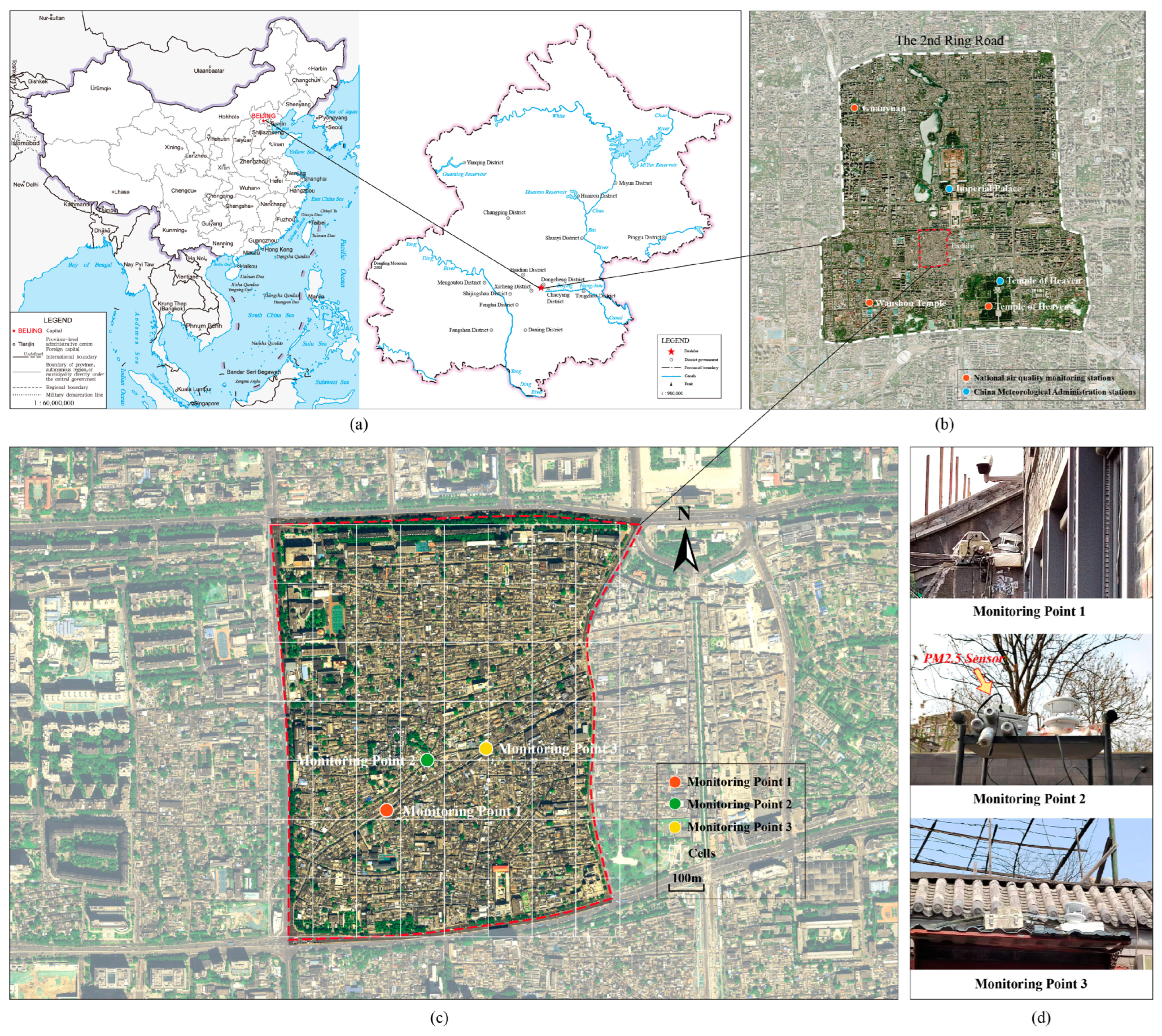
2.1. Study Area

Beijing is a typical high-density city. As the research area, Dashilar Historic Neighborhood is located in the center of Beijing’s second ring road, with high spatial density and severe PM_2.5 pollution [69]. It is a high-density living agglomeration, occupying a total area of 0.96 km² and extending for 1 km in length and 0.9 km in width (Figure 1). Due to protective height restriction policies implemented for historic preservation, this area has maintained high building density along with relatively low building height over an extended period, resulting in pollutant accumulation and dispersion patterns significantly different from typical modern urban areas. It exhibits typical characteristics of historic neighborhoods in the old city of Beijing, with frequent tourist visits, numerous commercial service facilities, high building density, low green coverage, and complex hutong texture as the main features. The study area is partitioned into 56 units of 120 m × 150 m granularity as the regression samples.

2.2. PM_2.5 Concentration Data

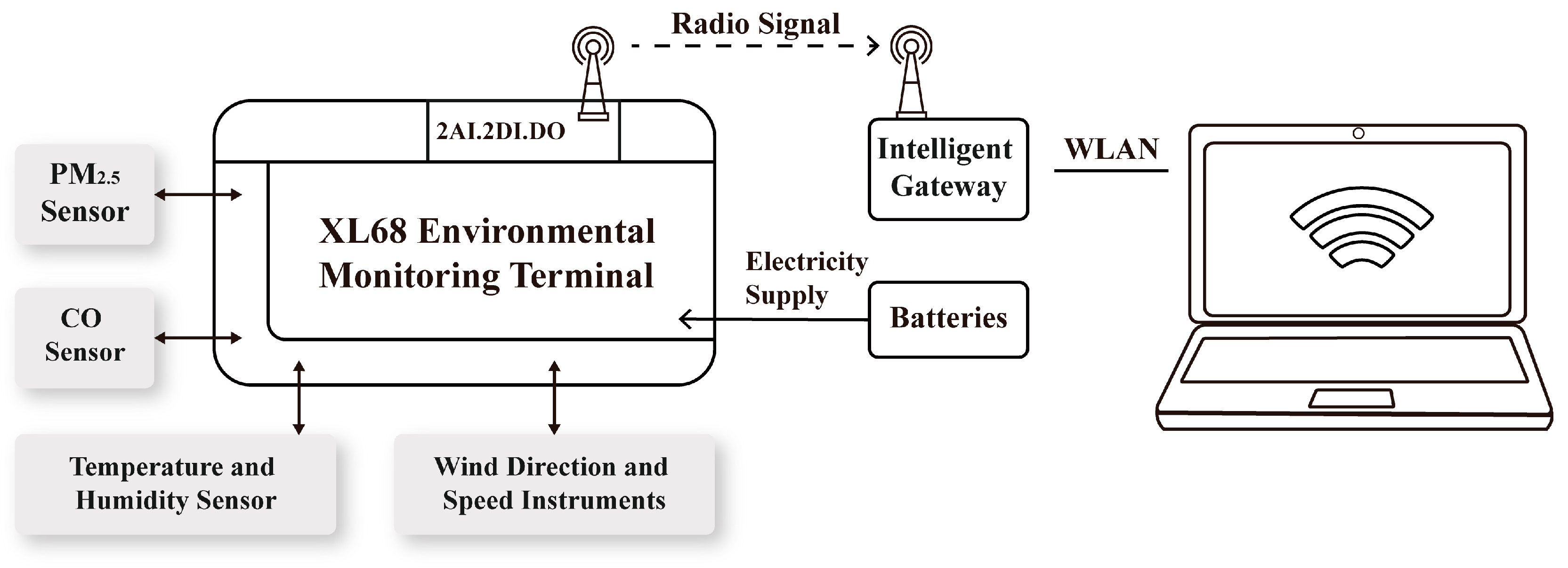
2.2.1. Monitoring of PM_2.5 Concentrations

The main microclimatic parameters and pollutant concentration were monitored by the XL68 of ambient on-line monitoring instruments; the recording interval was 2 s. Three points were selected following the Technical Regulation for Selection of Ambient Air Quality Monitoring Station (HJ664-2013) [70]. These monitoring points were carefully selected to reflect differences in population activity, commercial activity, building morphology, vegetation morphology, and road traffic morphology within the historic neighborhood. Specifically, monitoring point 1 was situated near an area characterized by higher traffic volume, point 2 was located within a more open space with greater population flow and commercial activities, and site 3 was positioned in an area exhibiting denser vegetation coverage. Such differentiation in site selection ensured the spatial representativeness of various environmental conditions within the historic neighborhood. According to the above-mentioned technical regulation, the monitoring sites should effectively represent the overall air quality status and trends in urban built-up areas, typically covering an effective radius ranging from 500 m to 4 km. Consequently, the three selected monitoring points adequately covered the entirety of the study area, ensuring scientific validity in terms of spatial scale, location, and the quantity of the monitoring sites.

The monitoring instruments are set up at a height of 2 m above the ground, with no obstacles blocking or preventing the normal flow of air in the surrounding area. Continuous sampling was carried out in the spring, summer, autumn, and winter for a total of 52 days. Data with a valid monitoring duration of more than 20 h were taken as valid daily monitoring data, and their arithmetic mean values were used as the daily average values of meteorological parameters and pollutant quality concentrations. Details of the monitoring instrument are shown in Figure 2 and

Table A1. Environmental monitoring equipment parameters.

Equipment Name	Principles	Range	Accuracy	Resolution
CO Sensor	Laser Principles	0–10,000 ppm	±2% FS	1 ppm
PM2.5 Sensor	Laser Principles	PM2.5: 0~1000 µg/m3	±10 µg/m3	1 µg/m3
Temperature and Humidity sensors	Electronic Sensing Principles	Temperature: −40~120 °C Humidity: 0–100% RH	±0.3 °C ±3% RH	0.1 °C 1% RH
Wind Direction and Speed Instruments	Ultrasound Principles	Wind Speed: 0~60 m/s Wind Direction: 0~359.9	±3%	0.1 m/s 0.1°

in Appendix A.

In addition, a comprehensive set of air quality and microclimate data were required to serve as background information for the subsequent modeling experiments. The air quality data were obtained from national air quality monitoring stations (https://data.epmap.org/product/nationair) (accessed on 27 April 2022), while the microclimate data were sourced from surface observations at China Meteorological Administration stations (http://data.cma.cn) (accessed on 27 April 2022). Considering the geographical location, wind direction, and surface characteristics of the study area, the average values of observed data from the Guanyuan, Temple of Heaven, and Wanshou Temple national monitoring stations were used as the background PM_2.5 concentrations for the Dashilar neighborhood. Similarly, the microclimate characteristics recorded by the Imperial Palace and Temple of Heaven meteorological stations were used as the background microclimate data. The locations of these stations are marked in Figure 1.

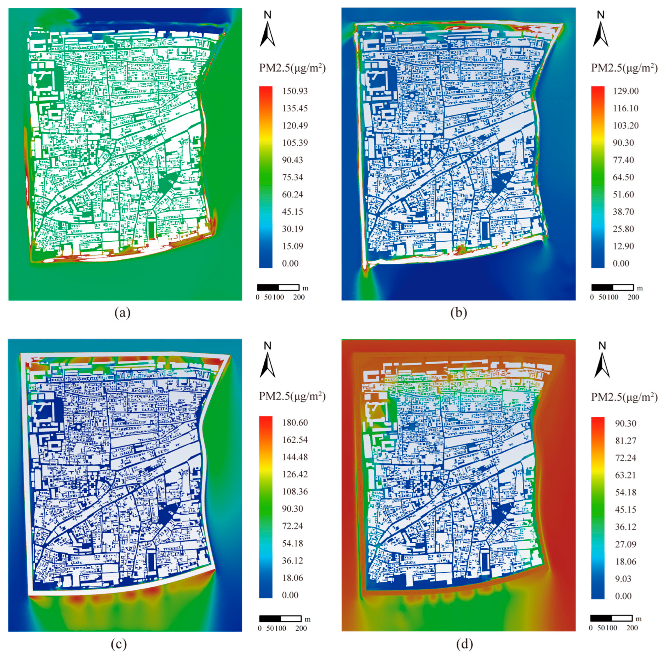
2.2.2. Numerical Simulation of CFD Model

The spatial and temporal dispersion of pollutants in the study area was simulated using ANSYS-Fluent 10.9 software. The simulation results were used to extract the average pollutant concentration data at 1.5 m pedestrian respiration height for 56 units. During the computational domain construction process, the simulation conditions were set with reference to the European cost best practice guideline [71]. The initial boundary conditions were based on the ground-based observation data from the Chinese meteorological stations, and the detailed parameters are shown in

Table 1. Set of parameters and boundary.

Boundary Condition	Parameters Settings
Inflow boundary	Wind speed: $U={\displaystyle \frac{U_{*}}{\kappa }}\ln \left({\displaystyle \frac{z+z_0}{z_0}}\right)$
	The turbulent kinetic energy: $(K={\displaystyle \raisebox{1ex}{$U_{*}^2$}\!\left/ \!\raisebox{-1ex}{$\sqrt{C_{\mu }}$}\right.})$
Exit boundary	Energy dissipation rate: $\epsilon =U_{*}^3\left[\kappa \left(Z+Z_0\right)\right]$
	${\displaystyle \frac{\vartheta }{{\vartheta }_x}}\left(u,\nu ,\omega ,k,\epsilon \right)=0$
Upper boundary and two sides boundary	$\omega =0$
	${\displaystyle \frac{\vartheta }{{\vartheta }_x}}\left(u,\nu ,\omega ,k,\epsilon \right)=0$
Lower boundary	Standard surface function: surface roughness thickness Ks = 0.0025 m, roughness constant Cs = 0.75
Building Surfaces	Standard surface function: Ks = 0.003 m, Cs = 0.75

where U is the horizontal wind speed at height z (m/s), U_∗ is ground friction speed (m/s), and κ is the Von·arman constant defined as 0.42. z₀ is surface roughness defined as 0.25. C_μ is a constant of the standard K-ε closing scheme and is defined as 0.09.

. The turbulence model is the $\kappa -\epsilon$ model, and the solution algorithm is the pressure-coupled AIMPLE algorithm (second-order windward mode). The simulation reaches convergence by default when the residual values of all variables are less than 10⁻³.

According to the actual situation of the study area, the 3D models of the neighborhood buildings, vegetation, and roads were established in SpaceClaim, and the non-smooth appearance is ignored on the basis of retaining the aggregate features. The computational domain was determined by the maximum building height, called Hmax. The final dimension of the computational domain was determined to be x × y × z = 1360 × 1460 × 180 m, while the horizontal and vertical spacing of the domain both maintain a distance of at least 5 H_max from the outermost points of the modeling range (Figure 3a). Non-structural meshing was used to delineate three sets of coarse, medium, and fine meshes, and a mesh-independence test was carried out. Ultimately, 2.2 × 108 meshes were divided, with the quality of the surface mesh exceeding 0.3 and the quality of the body mesh exceeding 0.2 (Figure 3b).

For the calculation, the air density was set to 1.189 kg/m³ under standard temperature and pressure conditions. The data from the national monitoring stations were adopted as the background input for the initial simulation. Field monitoring data collected within the Dashilar neighborhood were used to validate the simulation results and ensure their accuracy and reliability. Within each seasonal monitoring campaign, meteorological conditions and pollutant concentration variations exhibited only minor differences. After a comprehensive evaluation, four representative days, each corresponding to a typical season, were selected for simulation (Spring (28 March 2022), Summer (18 July 2021), Autumn (19 October 2022), and Winter (2 January 2022)). The detailed initial conditions for the CFD simulations are summarized in

Table A2. Initial condition setting of CFD simulation.

Dates	Wind Speed (m/s)	Wind Direction	Temperature (°C)	PM2.5 Concentration (μg/m3)
28 March 2022	1.5	S	9	53
18 July 2021	0.6	N	26	16
19 October 2022	1.1	N	10	6
2 January 2022	0.4	N	−3	11

.

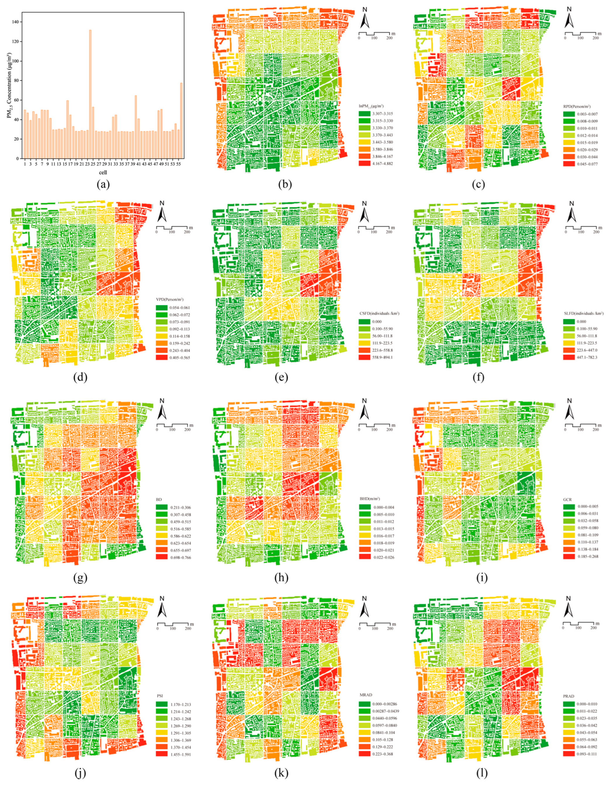
2.3. Independent Variables

Based on the previous research and considering the generation, absorption, dispersion, and removal mechanisms of PM_2.5, 10 urban density parameters were selected as independent variables in five aspects from a social-biophysical perspective [72,73,74,75,76]. The indicators were Residential Population Density (RPD), Visiting Population Density (VPD), Catering Service Facilities Density (CSFD), Shopping and Leisure Service Facilities Density (SLFD), Building Density (BD), Building Height Density (BHD), Green Coverage Rate (GCR), Patch Shape Index (PSI), Motorway Road Area Density (MRAD), and Pavement Road Area Density (PRAD) (

Table 2. Assumption of the relationships between PM_2.5 concentrations and urban morphology in neighborhood.

Metrics (Abbreviation)			Direction	Assumption
Socioeconomic dimension	Population Activity	Residential Population Density (RPD)	+	High RPD may add more household domestic emissions and thus increase air pollution [77].
			−	High RPD can reduce air pollution by encouraging the use of public transit [17].
		Visiting Population Density (VPD)	+	High VPD may increase all kinds of production and living activities and cause dust to fly up from the ground, which may increase PM2.5 concentrations [57].
	Commercial Activity	Catering Service Facilities Density (CSFD)	+	High CSFD directly causes air emissions by cooking, which increase PM2.5 concentrations [78].
		Shopping and Leisure Services Facilities Density (SLFD)	+	High SLFD can restrict airflow and increase the secondary pollutants generated by attracting a large number of people for a short period of time, which may increase PM2.5 concentrations.
Biophysical dimension	Building Morphology	Building Density (BD)	+	High BD may increase surface roughness and impede the dispersion of pollutants, which may increase PM2.5 concentrations [39].
			−	Low BD causes high wind speed due to lack of obstruction, which may cause dust accumulation and increase PM2.5 concentrations [8].
		Building Height Density (BHD)	+	High BHD produces a shading effect that delays the longwave radiation from the street canyons, which may increase the atmospheric turbulent energy and favor the vertical PM2.5 dispersion [75].
			−	High BHD may create an urban canyon effect, which may impede air circulation and increase PM2.5 concentrations.
	Vegetation Morphology	Green Coverage Rate (GCR)	−	High GCR absorbs and deposits more pollutants, which may decrease PM2.5 concentrations [48].
		Patch Shape Index (PSI)	+	High PSI may cause localized poor air circulation, making it difficult for pollutants to disperse, thus increasing PM2.5 concentrations [79].
			−	High PSI can provide more surface area in contact with the air, which promotes the adsorption and deposition of pollutants, thus reducing PM2.5 concentrations [53].
	Road Morphology	Motorway Road Area Density (MRAD)	+	More motorway roads, as emission sources, may increase PM2.5 concentrations [57].
		Pavement Road Area Density (PRAD)	−	More pavement roads allow for increased wind flow and accelerated dispersion of pollutants, which may decrease PM2.5 concentrations.

and

Table A4. Metrics used in the study.

Metrics		Expression		Description	Data Source
Population Activity	Residential Population Density (RPD)	$\mathrm{R}\mathrm{P}\mathrm{D}={\displaystyle \frac{N_{Rpop}}{S}}$	NRpop = Number of Residential Population S = Site area (m2)	Spatial distribution of the resident population	LBS data from China Unicom
	Visiting Population Density (VPD)	$\mathrm{V}\mathrm{P}\mathrm{D}={\displaystyle \frac{N_{Vpop}}{S}}$	NVpop = Number of Visiting Population S = Site area (m2)	Spatial distribution of the visiting population	LBS data from China Unicom
Commercial Activity	Catering Service Facilities Density (CSFD)	$CSFD={\displaystyle \frac{N_{csf}}{S}}$	Ncsf = Number of Catering Service Facilities S = Site area (km2)	Spatial distribution of the Catering Service Facilities	GaoDe Map POI data
	Shopping and Leisure Services Facilities Density (SLFD)	$SSFD={\displaystyle \frac{N_{ssf}}{S}}$	Nssf = Number of Shopping and Leisure Services Facilities S = Site area (km2)	Spatial distribution of Shopping and Leisure Services Facilities	GaoDe Map POI data
Building Morphology	Building Density (BD)	$BD={\displaystyle \frac{BA}{S}}$	BA = Building area (m2) S = Site area (m2)	Building congestion in the study area	2023 OpenStreetMap (OSM) data
	Building Height Density (BHD)	$BHD={\displaystyle \frac{\sum _{i=1}^n{H}_i}{n}}$	Hi = Building height (m) n = Number of buildings	Degree of spatial variation in building height	2023 OpenStreetMap (OSM) data
Vegetation Morphology	Green Coverage Rate (GCR)	$GCR={\displaystyle \frac{S_G}{S}}$	SG = Area covered by vegetation (m2) S = Site area (m2)	Vegetation cover density	2021 Remote sensing data from the French PNEO satellite
	Plaque Shape Index (PSI)	$\mathrm{P}\mathrm{S}\mathrm{I}={\displaystyle \frac{P}{2\sqrt{\pi A}}}$	P = plaque circumference of vegetation (m) A = Plaque area of vegetation (m2)	Compactness of vegetation patches	2021 Remote sensing data from the French PNEO satellite
Road Traffic Pattern	Motorway Road Area Density (MRAD)	$\mathrm{M}\mathrm{R}\mathrm{A}\mathrm{D}={\displaystyle \frac{S_{MR}}{S}}$	SMR = Motorway Area (m2) S = Site area (m2)	The range of scales of the surface space that the motorway road actually has	2023 OpenStreetMap (OSM) data
	Pavement Road Area Density PRAD)	$\mathrm{P}\mathrm{R}\mathrm{A}\mathrm{D}={\displaystyle \frac{S_{PR}}{S}}$	SPR = Pavement Area (m2) S = Site area (m2)	The range of scales of the surface space that the pavement road actually has	2023 OpenStreetMap (OSM) data

). Specifically, variables such as Building Density and Building Height Density directly capture the unique spatial textures and architectural forms shaped by historical preservation policies, whereas population and commercial activity indicators reflect the distinct urban vitality and intensity of human activities inherent to historic neighborhoods. Furthermore, Green Coverage Rate, Patch Shape Index and Road Area Density help interpret how limited green spaces and unique road structures influence the localized dispersion and accumulation processes of PM_2.5 pollution.

The Population Activity data were derived from the monthly aggregated Location-Based Services (LBS) data provided by China Unicom (https://www.chinaunicom.cn) in FY2023 with an accuracy of 120 m × 150 m. LBS data, which collects anonymized geolocation information from mobile devices, is commonly used to reflect population movement and spatial distribution. The Commercial Activity data were derived from the Points of Interest (POI) data categorized by GaoDe Map, which was corrected by an on-site survey. POI data includes geolocation and classification of urban facilities such as shops, restaurants, and service venues (https://lbs.amap.com/api/webservice/guide/api-advanced/search) (accessed on 12 April 2024). The Building Morphology data were supplied by the Beijing Municipal Institute of Surveying and Mapping in 2020 with the 2023 OpenStreetMap (OSM) data and on-site survey for verification. OSM is a collaborative global mapping platform that provides open-access geographic data contributed and updated by volunteers and communities worldwide (https://www.openstreetmap.org). The Vegetation Morphology data were based on the 0.3 m high-resolution remote sensing data acquired by the French PNEO satellite in September 2021. Preprocessing, decoding, and statistics of the data were handled by ENVI5.6 and ARCGIS10.8 software. The Road Morphology data were obtained from OSM data and combined with the Dashilar neighborhood road network planning and on-site survey to ensure accuracy. The attribute and classification were extracted by motorized and non-motorized lanes in ArcGIS.

2.4. Statistical Models

2.4.1. Pearson Correlation Analysis

Correlation analysis was conducted to assess the strength of linear correlation between all variables. As all variables were continuous numeric variables, Pearson correlation analysis was used instead of Spearman correlation analysis. It was employed to determine the urban density indicators that were correlated with PM_2.5 concentrations.

2.4.2. Least Absolute Shrinkage and Selection Operator

Due to the large number of independent variables and small sample size, the Lasso regression method was employed to improve the accuracy and interpretability of the model [80]. Lasso regression incorporates an L1-paradigm penalty term on the basis of OLS, which compels certain regression coefficients to decrease to zero, thereby enabling variable selection. The model can be presented by Equation (1):

$$min\left({\sum }_{i=1}^n{\left(y_i-{\sum }_{j=1}^p{X}_{ij}{\beta }_j\right)}^2+\lambda {\sum }_{j=1}^p\left|{\beta }_j\right|\right),$$

(1)

where $y_i$ is the i-th observed value of the dependent variable, $X_{ij}$ denotes the value of the j-th independent variable for the i-th observation, ${\beta }_j$ is the regression coefficient of the j-th independent variable, and $\lambda$ is the regularization parameter controlling the penalty intensity, n is the total number of observations, p is the total number of independent variables.

By adjusting the value of λ, the complexity of the model and the stringency of variable selection can be controlled. λ corresponding to the minimum mean square error (MSE) was chosen as the most optimal parameter using 10-fold cross-validation. The analysis was conducted in R studio using the “glmnet” package.

2.4.3. Quantile Regression

Traditional regression can estimate the conditional expectations of the dependent variables from the independent variables. In contrast, Quantile regression (QR) explores the relationship between the independent variables and the conditional quantiles of the dependent variables [81], which can estimate the effect of the independent variables on the dependent variables at each quantile τ. This is crucial for understanding the distributional characteristics of the dependent variables under different conditions as well as revealing their heterogeneous effects. The final model is as follows:

$$lnPM2.5={\beta }_1\left(\tau \right)X_{i1}+{\beta }_2\left(\tau \right)X_{i2}+{\beta }_3\left(\tau \right)X_{i3}+{\beta }_P\left(\tau \right)X_{iP}+\dots +{\epsilon }_i,$$

(2)

where lnPM_2.5 is the observed value of the dependent variables, X_i1, X_i2, … X_ip are the observed values of the independent variables, ${\beta }_1\left(\tau \right)$, ${\beta }_2\left(\tau \right)$, ${\beta }_3\left(\tau \right)$, ${\beta }_P\left(\tau \right)$ are the coefficients under the quantile τ, and ${\epsilon }_i$ is the error term denoting the unobserved random influences.

The QR was estimated by bootstrap intensive algorithmic technique by stata18. Following the general research practice, four typical quantiles (25th, 50th, 75th, and 90th quantiles) were selected [63].

Additionally, the Sobel Test mediated effect test was used to test the mediated effect of building density on PM_2.5 concentrations by influencing temperature, as described in Appendix A Stata18 Sobel Test Mediation effects test code: sgmediation lnpm25,mv(temp) iv(BD).

3. Results

3.1. Results of Air Monitoring and Numerical Simulation

Neighborhood PM_2.5 monitoring data were obtained for a total of 52 days during the monitoring period of 10 July 2021 to 8 April 2022, and data from nearby state control stations were recorded for the same period. As illustrated in Figure 4, according to the Ambient Air Quality Standards (GB3095-2012) [82], the daily average PM_2.5 concentration exceeded the national primary standard for half of the monitoring period. The neighborhood was subjected to relatively severe air pollution.

The simulated pollutant concentration data were calibrated against the monitored values, and a t-test was applied to determine if there was a significant difference between the monitored and simulated values. The results and specific explanations can be found in Appendix A and

Table A3. Error test of simulation results.

Variables	Difference in Value					t	Sig. Double
	Mean	Standard Deviation	Standard Error of the Mean	95% Confidence Interval
				Lower Limit	Upper Limit
PM2.5	3.615653	2.5167146	0.1317931	−0.657465	0.4681257	1.528	0.135

. This result confirmed the stability and robustness of the simulation data.

The PM_2.5 simulation results for the four seasons indicated that the areas with high pollution values were more likely to be concentrated in and around road emission sources (Figure 5). The concentrations of pollutants were highest in the periphery of the neighborhoods and varied considerably from one location to another, with areas of high, medium, and low pollution simultaneously. In summary, significant spatial heterogeneity was observed in the distribution of PM_2.5 in the neighborhood; the unknown relationship between PM_2.5 pollution and urban density characteristics at the neighborhood scale remains to be investigated.

3.2. Spatial Distribution and Descriptive Statistical Analysis

Based on the spatial distribution (Figure 6), VPD distribution exhibited high spatial heterogeneity with high outside and low inside, and high in the east and low in the west. The commercial activities in the neighborhood were distributed in a clustered manner, with the right side of the street area being the primary concentration of frequent commercial activities. BD was characterized by high inside and low outside, as well as high east and low west. The neighborhood’s vegetation was primarily located on the north and east sides, and the GCR and PSI varied significantly between various units, overshowing the characteristics of a uniformly low interior and a high outside. The distribution characteristics of PRAD in the study area were comparable to those of BD, which was also distinguished by a high interior and a low exterior, as well as a high east side and a low west side.

Based on the mathematical statistics (

Table 3. Descriptive statistical analysis of variables.

Variable Type		Metrics	Units	Minimum	Maximum	Median	Mean	Standard Deviation
Explained variable	PM2.5 concentration	PM2.5	µg/m3	27.299	131.844	29.517	37.957	16.959
		lnPM2.5	µg/m3	3.307	4.882	3.385	3.573	0.326
Explanatory variables	Population activity	RPD	Person/m2	0.003	0.077	0.013	0.019	0.016
		VPD	Person/m2	0.054	0.565	0.111	0.151	0.122
	Commercial activity	CSFD	individuals/km2	0.000	894.154	55.885	122.747	218.088
		SLFD	individuals/km2	0.000	782.385	55.885	119.753	160.318
	Building morphology	BD	——	0.211	0.766	0.608	0.564	0.115
		BHD	m/m2	0.004	0.026	0.015	0.015	0.005
	Vegetation Morphology	GCR	——	0.005	0.268	0.067	0.084	0.060
		PSI	——	1.170	1.591	1.291	1.324	0.102
	Road Morphology	MRAD	——	0.000	0.368	0.068	0.090	0.089
		PRAD	——	0.000	0.111	0.042	0.044	0.030

), the average RPD in the study area was slightly lower than that of the entire Xicheng District, which is the administrative district where the Dashilar neighborhood is located. In contrast, the average VPD in the neighborhood was approximately eight times that of RPD. The study area was classified as a high-building-density neighborhood, with an average BD of 56.4%. The value was significantly higher than the general construction standards for modern neighborhoods. Additionally, there was a significant disparity between the highest and lowest values of BD in the units. The neighborhood’s verdant vegetation was generally low, with an average GCR of 8.4%, which was significantly lower than the standards for general modern neighborhoods in the design code for residential areas [83].

3.3. Results of Pearson Correlation Analysis

A total of seven indicators with correlation to PM_2.5 concentration were selected (Figure 7a). The results of correlation analysis demonstrated that VPD, BD, GCR, PSI, SLFD, and MRAD were correlated with PM_2.5 concentration at the level of 0.001. Additionally, CSFD and PM_2.5 concentration were correlated at the level of 0.05. There was no correlation between RPD, BHD, PRAD, and PM_2.5 concentration.

3.4. LASSO Regression

The CV residual plot was illustrated in Figure 7b, where the horizontal axis represents the logarithm of the Lasso regression parameter λ, and the vertical axis shows the mean squared error (MSE) of the Lasso regression model for different values of λ. The result indicated that the model achieved the lowest MSE when log(λ) = −4.337291 (corresponding to λ = 0.01434581). At this point, the model identified four key variables influencing PM_2.5 concentration: VPD, BD, PSI, and SLFD (Figure 7c). Specifically, the findings indicated that the concentration of PM_2.5 was significantly positively influenced by VPD, PSI, and SLFD, while the concentration of PM_2.5 was significantly negatively influenced by BD. The indicators in the model were ranked in order of relative importance: BD, VPD, SLFD, and PSI (

Table 4. Significant variables and their regression coefficients selected for LASSO regression.

Metrics	Coefficient
VPD	0.08966835
SLFD	0.08177266
BD	−0.14191426
PSI	0.08136056
Intercept	3.57270579

).

3.5. Results of Quantile Regression

The multicollinearity test results for the explanatory variables were summarized in

Table A6. OLS regression and Multi-collinearity test of explanatory variables (PD, BD, PSI, CSF, SSF, and LSF) in model.

R2	0.7409
Adjusted R2	0.7206
Root MSE	0.17398
Variables	Coefficient	Standard error	t-value	Prob (>|t|)		VIF
VPD	0.0942529	0.0328049	2.87	0.006	**	1.96
BD	−0.1508619	0.0343236	−4.40	0.000	***	2.14
SLFD	0.0944151	0.0328119	2.88	0.006	**	1.96
PSI	0.0898761	0.0344049	2.61	0.012	*	2.15
cons	3.572706	0.0232497	153.67	0.000

*** p < 0.001; ** p < 0.01; * p < 0.05 (2-tailed).

. It was obvious that the VIF values of all explanatory variables were in the range of 1.96 to 2.15, all of which were less than 5. Consequently, the model passed the multicollinearity test. Moreover, the blue density curves in Figure 8 are nearly all deviating from the red fitted line, which suggests that the variables were not normally distributed. Therefore, QR was a more reasonable and robust approach than OLS.

In accordance with general practice, five typical quantiles (25th, 50th, 75th, 90th) were selected for evaluation in this study. The 56 regression samples were classified into five groups based on their annual average PM_2.5 concentration (

Table A7. Grades based on PM_2.5 pollution.

Quantile	Grading Interval of LnPM2.5	Cells
The lower 25th quantile grade	[0, 3.329)	38, 30, 27, 34, 36, 29, 37, 52, 47, 39, 28, 20, 51, 50
The 25–50th quantile grade	[3.329, 3.385)	35, 42, 43, 44, 19, 45, 22, 46, 26, 31, 21, 23, 53, 12
The 50–75th quantile grade	[3.385, 3.807)	11, 55, 14, 13, 15, 18, 54, 3, 41, 6, 10, 32, 33, 17
The 75–90th quantile grade	[3.807, 3.917)	5, 2, 4, 48, 9, 8, 1, 7
The upper 90th quantile grade	[3.917)	49, 25, 16, 40, 56, 24

).

Table 5. Regression results of quantile and ordinary least squares.

Variables	QR				OLS
	25th Quantile	50th Quantile	75th Quantile	90th Quantile
Z_VPD	0.0756 * (0.0384)	0.0879 (0.0601)	0.1832 ** (0.0768)	0.1578 * (0.0905)	0.0943 *** (0.0328)
Z_SLFD	0.0484 (0.0519)	0.0226 (0.0605)	0.0947 (0.0775)	0.1406 (0.0928)	0.0944 *** (0.0328)
Z_BD	−0.1678 *** (0.0380)	−0.1494 *** (0.0347)	−0.1877 *** (0.0467)	−0.1527 * (0.0778)	−0.1509 *** (0.0343)
Z_PSI	0.0418 (0.0562)	0.0919 ** (0.0442)	0.0647 * (0.0339)	0.0747 (0.0628)	0.0899 ** (0.0344)
Intercept	3.4866 *** (0.0272)	3.5557 *** (0.0325)	3.7001 *** (0.0497)	3.7511 *** (0.0564)	3.5727 *** (0.0232)
Pseudo R2	0.3438	0.5232	0.5645	0.6125	0.7206

Notes: The values in parentheses represent standard errors. *, **, and *** indicate that variables passed a significant test at 10%, 5%, and 1% significant levels, respectively.

presented QR results and OLS regression estimations for comparison. As shown by Table 5, the majority of the independent variables passed the significance test at various quantile levels.

The 95% confidence intervals of QR were displayed and could be compared to the confidence intervals obtained through OLS regression (Figure 9). QR (between the two blue straight lines) and OLS regression (between the two red dashed lines) yielded significantly different confidence intervals. The OSL regression model only provided the average effect of the explanatory variables on PM_2.5 pollution, whereas QR was able to reveal the heterogeneous effects of the explanatory variables on PM_2.5 pollution in units with varying pollution levels.

4. Discussion

This investigation examined the correlation between annual average PM_2.5 concentrations and urban density at the neighborhood level. The study’s findings indicated that urban density was statistically substantially correlated with PM_2.5 concentrations at the neighborhood scale. However, the strength of this correlation was contingent upon the quantile level at which the PM_2.5 concentrations were located and the type of urban density metric used.

4.1. The Mechanism of Urban Density on PM_2.5

4.1.1. The Impact of Population Activity on PM_2.5 Concentration

The short-term human mobility represented by the VPD was the second main factor contributing to the increase in PM_2.5 concentration, which had a substantial positive impact on PM_2.5. This finding provides substantial evidence for the relationship between urban short-term human mobility and PM_2.5 at the neighborhood level. As a renowned tourist attraction and commercial hub in Beijing’s old city, Dashilar attracts substantial daily visitors, with average VPD approximately eight times higher than the RPD. This heavy visitor traffic increases both motor vehicle use and pedestrian movements, directly elevating local PM_2.5 levels through vehicle emissions and ground dust re-suspension [31,84]. Moreover, Dashilar’s characteristic narrow hutongs and compact street patterns further hinder pollutant dispersion, exacerbating the pollution caused by intensive human activities.

Conversely, the local RPD showed no significant correlation with PM_2.5 concentrations, possibly due to the specific urban evacuation policies applied in this area. Since 2017, the Beijing Municipal Government has implemented a targeted population-relocation policy in historic neighborhoods, significantly reducing local resident density [69,85]. This policy reduced household emissions within Dashilar, explaining the non-significant relationship between residential population density and PM_2.5.

4.1.2. The Impact of Commercial Activity on PM_2.5 Concentration

SLFD was the third main factor affecting PM_2.5 concentration and exerted a substantial positive influence on PM_2.5 concentration. This result reflects the unique commercial and spatial characteristics of the Dashilar Historic neighborhood. As a long-standing commercial hub in Beijing’s old city, Dashilar contains a dense concentration of shopping and leisure facilities within narrow and irregular road patterns. The coexistence of dense commercial facilities and insufficient traffic-carrying capacity frequently leads to traffic congestion due to the intensive use of private vehicles, delivery vehicles, and other modes of transportation, which is very likely to result in traffic congestion on the surrounding roads [84]. The traffic congestion and slow-moving vehicles produce more emissions than free-flowing traffic in commercial neighborhoods, which can lead to elevated pollution levels [32,86]. Furthermore, the dense road network lacks efficient ventilation pathways, hindering the dispersion of pollutants and amplifying the adverse effects of commercial activities on air quality. On the contrary, CSFD was excluded from the LASSO regression model as another indicator. It might be due to the strong spatial correlation between the two indicators (0.827 ***).

4.1.3. The Impact of Building Morphology on PM_2.5 Concentration

BD was the most important driving factor of pollutants and had a substantial negative impact on PM_2.5 concentration, which contradicted the findings of most previous research [62]. In general, low building density is often considered to enhance air circulation and promote the dispersion of pollutants due to reduced surface roughness [39]. However, this finding may be explained by the distinct spatial and morphological features of the Dashilar Historic neighborhood.

The negative impact of BD on PM_2.5 could be attributed to two potential mechanisms. Firstly, this study area is a representative historic neighborhood in the old city of Beijing. The average BD of the neighborhood is excessively high, and there are significant spatial differences with high inner and low outer. Consequently, the absence of effective blocking may result in strong winds exceeding the upper limit of the effective range, thereby generating particulate pollution [8]. Secondly, BD was found to have a mediating effect on PM_2.5 concentration by altering the temperature (see Stata18 Sobel Test Mediation effects test code: sgmediation lnpm25,mv(temp) iv(BD)).

It has been confirmed that the Dashilar neighborhood exhibited the highest UHI intensity within the old city of Beijing [68]. Specifically, the low BD areas at the periphery of this neighborhood receive direct solar radiation on the surface due to the lack of shading effect of building cover, resulting in an excessive local temperature increase [87,88,89,90]. Consequently, high temperatures are capable of increasing the production and volatilization of secondary pollutants such as O₃ and VOCs by accelerating photochemical reactions, thereby leading to an increase in the concentration of PM_2.5 [91]. In conclusion, the results inspire us to pay more attention to air pollution caused by high wind speeds and elevated temperatures induced by low-density spaces in high-density areas with substantial localized density disparities.

Conversely, there was no significant correlation between BHD and neighborhood PM_2.5 concentration. This may be attributed to the fact that the study area is a historic neighborhood in which building heights are strictly regulated [92]. Specifically, the buildings are primarily one-story bungalows with minimal spatial differentiation, and thus the three-dimensional density characteristics of the buildings are not significantly associated with PM_2.5.

4.1.4. The Impact of Vegetation Morphology on PM_2.5 Concentration

Previous studies have confirmed the impact of 2D Vegetation morphology on air pollution [93,94,95]. Most of the macro-level studies have shown that the complexity of Vegetation morphology is significantly and negatively correlated with PM_2.5 concentration [51]. It suggested that the complex morphology of vegetation patches could provide more surface area in contact with air, thus promoting the adsorption and deposition of atmospheric pollutants. However, different effects were found in Dashilar historic neighborhood. The PSI was the last main factor and positively correlated with PM_2.5, suggesting that complex vegetation patches impede the diffusion of neighborhood PM_2.5 concentrations. This phenomenon can be explained by the localized characteristics of Dashilar. First, this neighborhood exhibits extremely low vegetation coverage. The average GCR in this historic neighborhood is only 8.4%, which is substantially lower than the standard of no less than 30% in modern residential neighborhoods [83]. It has been demonstrated that the abatement of PM_2.5 is significant in neighborhoods with a diameter of 1 km when the GCR is between 25% and 35% [46]. However, in Dashilar, sparse and fragmented vegetation is mostly scattered in corner parks, narrow alleys, and courtyard gaps. Therefore, the small amount of vegetation with sporadic distribution has limited PM_2.5 deposition effect in the horizontal direction, and PM_2.5 deposited on the surface of leaves may be blown back to the air and suspended due to the wind flow.

Furthermore, the combination of complex vegetation patches and the street canyon effect caused by Dashilar’s dense and irregular hutong system leads to negative aerodynamic effects. In areas close to trees, complex patch shapes may disrupt vertical airflow, decreasing the upward wind speed and limiting the effective removal of pollutants [96]. This suggests that, in compact historic neighborhoods like Dashilar, poorly distributed and complexly shaped vegetation may even worsen PM_2.5 accumulation by obstructing ventilation paths.

4.2. Heterogeneous Effect of Urban Density on PM_2.5

The quantile regression results showed that both short-term human mobility density and PSI showed strong heterogeneous effects on PM_2.5 under different pollution levels, and the effect of BD on PM_2.5 showed strong homogeneous effects among different pollution levels.

The results showed that the influence of short-term human mobility represented by VPD on PM_2.5 increased slightly at first (between the 25th and 65th quantiles) and then increased rapidly (between the 65th and 95th quantiles) as pollution levels increased, indicating the areas with moderate pollution levels were the key areas to control PM_2.5. Air quality can be significantly damaged by only minor adjustments of the VPD when the pollution level was high, which is referred to as the marginal environmental damage. Generally, high VPD areas are accompanied by a large amount of traffic flow and commercial activities, which emit large amounts of pollutants [31]. When the pollutant concentration rose to high-level quantiles, even exceeding the self-purification capacity in the space, small changes in the VPD could lead to significant changes in PM_2.5 concentrations in these highly polluted areas [12]. Therefore, measures such as controlling the pedestrian flow and traffic flow density should be taken as soon as possible to effectively control PM_2.5 pollution to avoid severe pollution at a later stage (above the 90th quantile) [97,98].

The influence of BD on PM_2.5 fluctuated slightly with increasing quantile levels. BD showed a significant negative effect on PM_2.5 at all quantile levels, suggesting that there is a strong and consistent negative effect of BD on PM_2.5 throughout the distribution. On the one hand, the high BD area has difficult internal parking and well-developed external public transportation. These make the residents more likely to travel by bicycle or on foot in the internal high-BD areas and thus reduce the use of private vehicles and tailpipe emissions. On the other hand, the dense building layouts can change the local microclimates [40,41,90]. For example, lowering ground temperatures by increasing the building’s shaded area can help reduce the generation of secondary pollutants. These findings suggest that it is necessary to improve walking and cycling friendliness and encourage residents to choose green travel modes to reduce the impact of automobile emissions on PM_2.5. Additionally, it is crucial to consider the correlation between the architectural layout of neighborhoods and microclimate environments.

The influence of PSI on PM_2.5 showed an inverted ‘U’-shaped curvilinear development trend with the increase in quantile level. The influence of PSI on PM_2.5 was not significant in the 25th quantile of low pollution and the 90th quantile of high pollution but showed a significant positive influence and peaked at the 50th quantile. It is possible that the local microclimate changes have a more substantial impact on PM_2.5 concentrations at moderate pollution levels, which makes pollutants less likely to spread and increases the retention time of PM_2.5 [99]. Therefore, in medium-level pollution regions, the complexity of the outer contours of vegetation patches can be effectively reduced by frequent pruning of trees to regularize them or planting vegetation in geometric patterns, thereby reducing pollution. However, the study area is a well-preserved historic neighborhood in the core area of Beijing, and the courtyard texture is more complete [100]. Geometrically patterned tree planting is not aligned with the vegetation aesthetics in traditional Chinese landscaping and is difficult to integrate with the local physical environment texture [101]. It is more reasonable and effective to pursue alternative methods of reducing PM_2.5 concentrations.

4.3. Limitation and Future Directions

First, only one representative historic neighborhood was selected as the research object, and the minimal precision was a 120 m × 150 m granularity grid, resulting in a limited sample size. The follow-up investigation can consider selecting multiple neighborhoods as the research object to expand the data sample size and make the captured pattern more generalizable.

Second, our analysis specifically focused on urban density characteristics from a social-biophysical perspective, using ten selected variables to reflect influences on PM_2.5. While these indicators capture many essential factors, they can not fully encompass all unique morphological features of historic neighborhoods. For instance, additional morphological attributes such as spatial openness, building volume density, and road cumulative azimuth angle could also yield an understanding of how historic urban morphology impacts pollution. Future studies could incorporate these variables to provide a more comprehensive analysis.

Third, the mechanisms of PM_2.5 generation and formation are very complex, and this study mainly focuses on the correlation between urban density and PM_2.5 as well as spatial heterogeneous effects. Nevertheless, the generation and formation of PM_2.5 are also directly influenced by local microclimatic conditions, including temperature, humidity, wind direction, and wind speed. Moreover, these microclimatic factors are correlated with a variety of density indicators; thus, subsequent studies could explore the ternary relationship between these three dimensions in depth.

Furthermore, the PM_2.5 cross-sectional data used in this study were obtained by numerical simulation that used background concentrations from the national monitoring center, incorporating surrounding road emissions as well as neighborhood-scale building, vegetation, and road characteristics. However, our simulation process does not consider the influence of urban form elements of the adjacent neighborhoods, which may affect the accuracy of the simulation. While carefully selected three fixed monitoring stations were employed, further methodological improvements remain possible. Future research could adopt mobile or portable monitoring systems, higher-resolution sensors, or multi-source data collection for finer spatiotemporal resolution, thus better explaining how morphological characteristics of historic neighborhoods affect PM_2.5.

5. Conclusions

Many city neighborhoods worldwide are facing severe PM_2.5 pollution, which threatens human health. In this study, an integrated social-biophysical perspective was applied to quantify the impacts of population, commercial buildings, vegetation, and roads on PM_2.5 concentration in high-density historic neighborhoods. We found the main factors affecting PM_2.5 and analyzed the heterogeneous effects of these main factors on different PM_2.5 concentration levels at the neighborhood scale. The following main findings were found:

Population activity, Commercial activity, Building morphology, and Vegetation morphology all significantly affected neighborhood PM_2.5 levels, and four main factors that affected PM_2.5 concentrations were screened out.

In terms of Population activity, the short-term human mobility represented by the VPD was the second main factor contributing to the increase in PM_2.5 concentration and has a significantly positive influence on PM_2.5. The results of the heterogeneous effects suggested that the impact of VPD on PM_2.5 increased slightly at first (between the 25th and 65th quantiles) and then increased rapidly (between the 65th and 95th quantiles) as pollution levels increased, indicating the areas with moderate pollution levels were the key areas to control PM_2.5. For these areas, measures such as controlling the pedestrian flow and traffic flow density should be taken as soon as possible to effectively control PM_2.5 pollution to avoid severe pollution at a later stage (above the 90th quantile).

In terms of Commercial activity, SLFD was the third main factor, which has a positive effect on PM_2.5. The result demonstrated the importance of commercial activities for PM_2.5 control at the neighborhood level. Additionally, the QR result showed that the influence of SLFD on PM_2.5 was insignificant at all quantile levels, indicating no heterogeneous effect.

In terms of Building morphology, BD was the most important driving factor of pollutants in historic neighborhoods, which had a significant negative effect on PM_2.5. The QR results showed that BD showed a strong and consistent negative effect on PM_2.5 concentrations at all quantile levels, which indicates the homogeneity effect. It suggested that the influence of BD should be a concern in areas with all quantile pollution levels. Particular attention should be paid to the air pollution caused by high wind speeds and elevated temperatures induced by low building density.

In terms of Vegetation morphology, PSI was the last main factor that had a positive influence on PM_2.5, indicating the complex vegetation patterns in historic neighborhoods are not conducive to PM_2.5 dispersion. Moreover, the heterogeneous effect result showed that the influence of PSI on PM_2.5 showed an inverted ‘U’-shaped curvilinear relationship as the pollution level increased and peaked at the 50th quantile with moderate pollution, which was the key area to control PM_2.5.

References

1. Basu, S.; Nagendra, H.; Verburg, P.; Plieninger, T. Perceptions of Ecosystem Services and Knowledge of Sustainable Development Goals around Community and Private Wetlands Users in a Rapidly Growing City. Landsc. Urban Plan. 2024, 244, 104989. [Google Scholar] [CrossRef]
2. Huang, A.; Chu, M.; Cheng, W.; Wang, G.; Guan, P.; Zhang, L.; Jia, J. Dynamic Evaluation of China’s Atmospheric Environmental Pressure from 2008 to 2017: Trends and Drivers. J. Environ. Sci. 2025, 150, 177–187. [Google Scholar] [CrossRef]
3. Li, F.; Liu, X.; Hu, D.; Wang, R.; Yang, W.; Li, D.; Zhao, D. Measurement Indicators and an Evaluation Approach for Assessing Urban Sustainable Development: A Case Study for China’s Jining City. Landsc. Urban Plan. 2009, 90, 134–142. [Google Scholar] [CrossRef]
4. Patias, N.; Rowe, F.; Cavazzi, S.; Arribas-Bel, D. Sustainable urban development indicators in Great Britain from 2001 to 2016. Landsc. Urban Plan. 2021, 214, 104148. [Google Scholar] [CrossRef]
5. Ahn, H.; Lee, J.; Hong, A. Urban Form and Air Pollution: Clustering Patterns of Urban Form Factors Related to Particulate Matter in Seoul, Korea. Sustain. Cities Soc. 2022, 81, 103859. [Google Scholar] [CrossRef]
6. Lopes, D.; Ferreira, J.; Rafael, S.; Hoi, K.I.; Li, X.; Liu, Y.; Yuen, K.-V.; Mok, K.M.; Miranda, A.I. High-Resolution Multi-Scale Air Pollution System: Evaluation of Modelling Performance and Emission Control Strategies. J. Environ. Sci. 2024, 137, 65–81. [Google Scholar] [CrossRef]
7. Zhang, A.; Xia, C.; Li, W. Exploring the Effects of 3D Urban Form on Urban Air Quality: Evidence from Fifteen Megacities in China. Sustain. Cities Soc. 2022, 78, 103649. [Google Scholar] [CrossRef]
8. Yang, J.; Shi, B.; Shi, Y.; Marvin, S.; Zheng, Y.; Xia, G. Air Pollution Dispersal in High Density Urban Areas: Research on the Triadic Relation of Wind, Air Pollution, and Urban Form. Sustain. Cities Soc. 2020, 54, 101941. [Google Scholar] [CrossRef]
9. Cai, X.; Wu, Z.; Cheng, J. Using Kernel Density Estimation to Assess the Spatial Pattern of Road Density and Its Impact on Landscape Fragmentation. Int. J. Geogr. Inf. Sci. 2013, 27, 222–230. [Google Scholar] [CrossRef]
10. Wang, C.; Wu, Y.; Shi, X.; Li, Y.; Zhu, S.; Jin, X.; Zhou, X. Dynamic Occupant Density Models of Commercial Buildings for Urban Energy Simulation. Build. Environ. 2020, 169, 106549. [Google Scholar] [CrossRef]
11. Wu, J.; Ma, L.; Li, W.; Peng, J.; Liu, H. Dynamics of Urban Density in China: Estimations Based on DMSP/OLS Nighttime Light Data. IEEE J. Sel. Topics Appl. Earth Observ. Remote Sens. 2014, 7, 4266–4275. [Google Scholar] [CrossRef]
12. Wang, S.; Xu, L.; Ge, S.; Jiao, J.; Pan, B.; Shu, Y. Driving Force Heterogeneity of Urban PM2.5 Pollution: Evidence from the Yangtze River Delta, China. Ecol. Indic. 2020, 113, 106210. [Google Scholar] [CrossRef]
13. Chen, J.; Wang, B.; Huang, S.; Song, M. The Influence of Increased Population Density in China on Air Pollution. Sci. Total Environ. 2020, 735, 139456. [Google Scholar] [CrossRef]
14. Gouveia, N.; Kephart, J.L.; Dronova, I.; McClure, L.; Granados, J.T.; Betancourt, R.M.; O’Ryan, A.C.; Texcalac-Sangrador, J.L.; Martinez-Folgar, K.; Rodriguez, D.; et al. Ambient Fine Particulate Matter in Latin American Cities: Levels, Population Exposure, and Associated Urban Factors. Sci. Total Environ. 2021, 772, 145035. [Google Scholar] [CrossRef] [PubMed]
15. Lee, C. How do built environments measured at two scales influence PM2.5 concentrations? Transp. Res. D Transp. Environ. 2021, 99, 103014. [Google Scholar] [CrossRef]
16. Stone, B. Urban Sprawl and Air Quality in Large US Cities. J. Environ. Manag. 2008, 86, 688–698. [Google Scholar] [CrossRef]
17. Lee, C. Impacts of Multi-Scale Urban Form on PM2.5 Concentrations Using Continuous Surface Estimates with High-Resolution in U.S. Metropolitan Areas. Landsc. Urban Plan. 2020, 204, 103935. [Google Scholar] [CrossRef]
18. Wang, H.; Li, J.; Gao, Z.; Yim, S.H.L.; Shen, H.; Ho, H.C.; Li, Z.; Zeng, Z.; Liu, C.; Li, Y.; et al. High-Spatial-Resolution Population Exposure to PM2.5 Pollution Based on Multi-Satellite Retrievals: A Case Study of Seasonal Variation in the Yangtze River Delta, China in 2013. Remote Sens. 2019, 11, 2724. [Google Scholar] [CrossRef]
19. Apergis, N.; Ozturk, I. Testing Environmental Kuznets Curve Hypothesis in Asian Countries. Ecol. Indic. 2015, 52, 16–22. [Google Scholar] [CrossRef]
20. Aşıcı, A.A.; Acar, S. Does income growth relocate ecological footprint? Ecol. Indic. 2016, 61, 707–714. [Google Scholar] [CrossRef]
21. Lin, B.; Zhu, J. Changes in Urban Air Quality during Urbanization in China. J. Clean. Prod. 2018, 188, 312–321. [Google Scholar] [CrossRef]
22. McCarty, J.; Kaza, N. Urban Form and Air Quality in the United States. Landsc. Urban Plan. 2015, 139, 168–179. [Google Scholar] [CrossRef]
23. Wang, Q.; Wang, X.; Li, R. Does Urbanization Redefine the Environmental Kuznets Curve? An Empirical Analysis of 134 Countries. Sustain. Cities Soc. 2022, 76, 103382. [Google Scholar] [CrossRef]
24. Gariazzo, C.; Pelliccioni, A.; Bolignano, A. A Dynamic Urban Air Pollution Population Exposure Assessment Study Using Model and Population Density Data Derived by Mobile Phone Traffic. Atmos. Environ. 2016, 131, 289–300. [Google Scholar] [CrossRef]
25. Park, Y.M.; Kwan, M.-P. Individual Exposure Estimates May Be Erroneous When Spatiotemporal Variability of Air Pollution and Human Mobility Are Ignored. Health Place 2017, 43, 85–94. [Google Scholar] [CrossRef]
26. Cui, C.; Wang, Z.; He, P.; Yuan, S.; Niu, B.; Kang, P.; Kang, C. Escaping from Pollution: The Effect of Air Quality on Inter-City Population Mobility in China. Environ. Res. Lett. 2019, 14, 124025. [Google Scholar] [CrossRef]
27. He, G.; Pan, Y.; Tanaka, T. The Short-Term Impacts of COVID-19 Lockdown on Urban Air Pollution in China. Nat. Sustain. 2020, 3, 1005–1011. [Google Scholar] [CrossRef]
28. Volke, M.I.; Abarca-del-Rio, R.; Ulloa-Tesser, C. Impact of Mobility Restrictions on NO2 Concentrations in Key Latin American Cities during the First Wave of the COVID-19 Pandemic. Urban Clim. 2023, 48, 101412. [Google Scholar] [CrossRef]
29. Wei, L.; Donaire-Gonzalez, D.; Helbich, M.; Van Nunen, E.; Hoek, G.; Vermeulen, R.C.H. Validity of Mobility-Based Exposure Assessment of Air Pollution: A Comparative Analysis with Home-Based Exposure Assessment. Environ. Sci. Technol. 2024, 58, 10685–10695. [Google Scholar] [CrossRef]
30. Yu, X.; Ivey, C.; Huang, Z.; Gurram, S.; Sivaraman, V.; Shen, H.; Eluru, N.; Hasan, S.; Henneman, L.; Shi, G.; et al. Quantifying the Impact of Daily Mobility on Errors in Air Pollution Exposure Estimation Using Mobile Phone Location Data. Environ. Int. 2020, 141, 105772. [Google Scholar] [CrossRef]
31. Boniardi, L.; Borghi, F.; Straccini, S.; Fanti, G.; Campagnolo, D.; Campo, L.; Olgiati, L.; Lioi, S.; Cattaneo, A.; Spinazzè, A.; et al. Commuting by Car, Public Transport, and Bike: Exposure Assessment and Estimation of the Inhaled Dose of Multiple Airborne Pollutants. Atmos. Environ. 2021, 262, 118613. [Google Scholar] [CrossRef]
32. Tomar, G.; Nagpure, A.S.; Kumar, V.; Jain, Y. High Resolution Vehicular Exhaust and Non-Exhaust Emission Analysis of Urban-Rural District of India. Sci. Total Environ. 2022, 805, 150255. [Google Scholar] [CrossRef]
33. Hoek, G.; Beelen, R.; De Hoogh, K.; Vienneau, D.; Gulliver, J.; Fischer, P.; Briggs, D. A Review of Land-Use Regression Models to Assess Spatial Variation of Outdoor Air Pollution. Atmos. Environ. 2008, 42, 7561–7578. [Google Scholar] [CrossRef]
34. Weber, N.; Haase, D.; Franck, U. Assessing Modelled Outdoor Traffic-Induced Noise and Air Pollution around Urban Structures Using the Concept of Landscape Metrics. Landsc. Urban Plan. 2014, 125, 105–116. [Google Scholar] [CrossRef]
35. Deng, X.; Cao, Q.; Wang, L.; Wang, W.; Wang, S.; Wang, S.; Wang, L. Characterizing Urban Densification and Quantifying Its Effects on Urban Thermal Environments and Human Thermal Comfort. Landsc. Urban Plan. 2023, 237, 104803. [Google Scholar] [CrossRef]
36. Liu, C.; Henderson, B.H.; Wang, D.; Yang, X.; Peng, Z. A Land Use Regression Application into Assessing Spatial Variation of Intra-Urban Fine Particulate Matter (PM2.5) and Nitrogen Dioxide (NO2) Concentrations in City of Shanghai, China. Sci. Total Environ. 2016, 565, 607–615. [Google Scholar] [CrossRef]
37. Ke, B.; Hu, W.; Huang, D.; Zhang, J.; Lin, X.; Li, C.; Jin, X.; Chen, J. Three-Dimensional Building Morphology Impacts on PM2.5 Distribution in Urban Landscape Settings in Zhejiang, China. Sci. Total Environ. 2022, 826, 154094. [Google Scholar] [CrossRef]
38. Shi, Y.; Xie, X.; Fung, J.C.-H.; Ng, E. Identifying Critical Building Morphological Design Factors of Street-Level Air Pollution Dispersion in High-Density Built Environment Using Mobile Monitoring. Build. Environ. 2018, 128, 248–259. [Google Scholar] [CrossRef]
39. Jiang, Z.; Cheng, H.; Zhang, P.; Kang, T. Influence of Urban Morphological Parameters on the Distribution and Diffusion of Air Pollutants: A Case Study in China. J. Environ. Sci. 2021, 105, 163–172. [Google Scholar] [CrossRef]
40. Cao, Q.; Luan, Q.; Liu, Y.; Wang, R. The Effects of 2D and 3D Building Morphology on Urban Environments: A Multi-Scale Analysis in the Beijing Metropolitan Region. Build. Environ. 2021, 192, 107635. [Google Scholar] [CrossRef]
41. Du, H.; Savory, E.; Perret, L. Effect of Morphology and an Upstream Tall Building on the Mean Turbulence Statistics of a Street Canyon Flow. Build. Environ. 2023, 241, 110428. [Google Scholar] [CrossRef]
42. Lu, D.; Mao, W.; Yang, D.; Zhao, J.; Xu, J. Effects of Land Use and Landscape Pattern on PM2.5 in Yangtze River Delta, China. Atmos. Pollut. Res. 2018, 9, 705–713. [Google Scholar] [CrossRef]
43. Tallis, M.; Taylor, G.; Sinnett, D.; Freer-Smith, P. Estimating the Removal of Atmospheric Particulate Pollution by the Urban Tree Canopy of London, under Current and Future Environments. Landsc. Urban Plan. 2011, 103, 129–138. [Google Scholar] [CrossRef]
44. Yan, J.; Chen, W.Y.; Zhang, Z.; Zhao, W.; Liu, M.; Yin, S. Mitigating PM2.5 Exposure with Vegetation Barrier and Building Designs in Urban Open-Road Environments Based on Numerical Simulations. Landsc. Urban Plan. 2024, 241, 104918. [Google Scholar] [CrossRef]
45. Chen, H.-S.; Lin, Y.-C.; Chiueh, P.-T. High-Resolution Spatial Analysis for the Air Quality Regulation Service from Urban Vegetation: A Case Study of Taipei City. Sustain. Cities Soc. 2022, 83, 103976. [Google Scholar] [CrossRef]
46. Chen, M.; Dai, F.; Yang, B.; Zhu, S. Effects of Neighborhood Green Space on PM2.5 Mitigation: Evidence from Five Megacities in China. Build. Environ. 2019, 156, 33–45. [Google Scholar] [CrossRef]
47. Zhang, X.; Du, J.; Huang, T.; Zhang, L.; Gao, H.; Zhao, Y.; Ma, J. Atmospheric Removal of PM 2.5 by Man-Made Three Northern Regions Shelter Forest in Northern China Estimated Using Satellite Retrieved PM 2.5 Concentration. Sci. Total Environ. 2017, 593–594, 713–721. [Google Scholar] [CrossRef]
48. Zhang, Y.; Zhang, T.; Zeng, Y.; Cheng, B.; Li, H. Designating National Forest Cities in China: Does the Policy Improve the Urban Living Environment? For. Policy Econ. 2021, 125, 102400. [Google Scholar] [CrossRef]
49. Zhou, Y.; Liu, H.; Zhou, J.; Xia, M. GIS-Based Urban Afforestation Spatial Patterns and a Strategy for PM2.5 Removal. Forests 2019, 10, 875. [Google Scholar] [CrossRef]
50. Rogan, J.E.; Lacher, T.E. Impacts of Habitat Loss and Fragmentation on Terrestrial Biodiversity. In Reference Module in Earth Systems and Environmental Sciences; Elsevier: Amsterdam, The Netherlands, 2018; p. B9780124095489109133. ISBN 978-0-12-409548-9. [Google Scholar]
51. Cao, W.; Zhou, W.; Yu, W.; Wu, T. Combined Effects of Urban Forests on Land Surface Temperature and PM2.5 Pollution in the Winter and Summer. Sustain. Cities Soc. 2024, 104, 105309. [Google Scholar] [CrossRef]
52. Zhai, C.; Bao, G.; Zhang, D.; Sha, Y. Urban Forest Locations and Patch Characteristics Regulate PM2.5 Mitigation Capacity. Forests 2022, 13, 1408. [Google Scholar] [CrossRef]
53. Chen, M.; Dai, F.; Yang, B.; Zhu, S. Effects of Urban Green Space Morphological Pattern on Variation of PM2.5 Concentration in the Neighborhoods of Five Chinese Megacities. Build. Environ. 2019, 158, 1–15. [Google Scholar] [CrossRef]
54. Xue, F.; Li, X. The Impact of Roadside Trees on Traffic Released PM 10 in Urban Street Canyon: Aerodynamic and Deposition Effects. Sustain. Cities Soc. 2017, 30, 195–204. [Google Scholar] [CrossRef]
55. Lee, J.-H.; Wu, C.-F.; Hoek, G.; De Hoogh, K.; Beelen, R.; Brunekreef, B.; Chan, C.-C. LUR Models for Particulate Matters in the Taipei Metropolis with High Densities of Roads and Strong Activities of Industry, Commerce and Construction. Sci. Total Environ. 2015, 514, 178–184. [Google Scholar] [CrossRef] [PubMed]
56. Shin, H.; Hyun, M.; Jeong, S.; Ryu, H.; Lee, M.G.; Chung, W.; Hong, J.; Kwon, J.-T.; Lee, J.; Kim, Y. A Correlation Study of Road Dust Pollutants, Tire Wear Particles, Air Quality, and Traffic Conditions in the Seoul (South Korea). Atmos. Pollut. Res. 2024, 15, 102309. [Google Scholar] [CrossRef]
57. Jareemit, D.; Liu, J.; Srivanit, M. Modeling the Effects of Urban Form on Ventilation Patterns and Traffic-Related PM2.5 Pollution in a Central Business Area of Bangkok. Build. Environ. 2023, 244, 110756. [Google Scholar] [CrossRef]
58. Zhao, X.; Zhou, W.; Han, L. The Spatial and Seasonal Complexity of PM2.5 Pollution in Cities from a Social-Ecological Perspective. J. Clean. Prod. 2021, 309, 127476. [Google Scholar] [CrossRef]
59. Zhou, C.; Chen, J.; Wang, S. Examining the Effects of Socioeconomic Development on Fine Particulate Matter (PM2.5) in China’s Cities Using Spatial Regression and the Geographical Detector Technique. Sci. Total Environ. 2018, 619–620, 436–445. [Google Scholar] [CrossRef]
60. Chen, M.; Bai, J.; Zhu, S.; Yang, B.; Dai, F. The Influence of Neighborhood-Level Urban Morphology on PM2.5 Variation Based on Random Forest Regression. Atmos. Pollut. Res. 2021, 12, 101147. [Google Scholar] [CrossRef]
61. Gao, Y.; Wang, Z.; Li, C.; Zheng, T.; Peng, Z.-R. Assessing Neighborhood Variations in Ozone and PM2.5 Concentrations Using Decision Tree Method. Build. Environ. 2021, 188, 107479. [Google Scholar] [CrossRef]
62. Yang, J.; Shi, B.; Zheng, Y.; Shi, Y.; Xia, G. Urban Form and Air Pollution Disperse: Key Indexes and Mitigation Strategies. Sustain. Cities Soc. 2020, 57, 101955. [Google Scholar] [CrossRef]
63. Yan, D.; Ren, X.; Kong, Y.; Ye, B.; Liao, Z. The Heterogeneous Effects of Socioeconomic Determinants on PM2.5 Concentrations Using a Two-Step Panel Quantile Regression. Appl. Energy 2020, 272, 115246. [Google Scholar] [CrossRef]
64. Zou, Q.; Shi, J. The Heterogeneous Effect of Socioeconomic Driving Factors on PM2.5 in China’s 30 Province-Level Administrative Regions: Evidence from Bayesian Hierarchical Spatial Quantile Regression. Environ. Pollut. 2020, 264, 114690. [Google Scholar] [CrossRef] [PubMed]
65. Che, W.; Zhang, Y.; Lin, C.; Fung, Y.H.; Fung, J.C.H.; Lau, A.K.H. Impacts of Pollution Heterogeneity on Population Exposure in Dense Urban Areas Using Ultra-Fine Resolution Air Quality Data. J. Environ. Sci. 2023, 125, 513–523. [Google Scholar] [CrossRef]
66. Jean-Pierre, F. Identification of Treatment Effects Using Control Functions in Models With Continuous, Endogenous Treatment and Heterogeneous Effects. Econometrica 2008, 76, 1191–1206. [Google Scholar] [CrossRef]
67. Gao, Y.; Wang, Z.; Liu, C.; Peng, Z.-R. Assessing Neighborhood Air Pollution Exposure and Its Relationship with the Urban Form. Build. Environ. 2019, 155, 15–24. [Google Scholar] [CrossRef]
68. Su, W.; Zhang, L.; Chang, Q. Nature-Based Solutions for Urban Heat Mitigation in Historical and Cultural Block: The Case of Beijing Old City. Build. Environ. 2022, 225, 109600. [Google Scholar] [CrossRef]
69. Beijing’s Urban Master Plan(2016–2035); China Architecture & Building Press: Beijing, China, 2019.
70. Technical Regulation for Selection of Ambient Air Quality Monitoring Station; China Environmental Science Press: Beijing, China, 2013.
71. Franke, J.; Hellsten, A.; Schlunzen, K.H.; Carissimo, B. The COST 732 Best Practice Guideline for CFD Simulation of Flows in the Urban Environment: A Summary. Int. J. Environ. Pollut. 2011, 44, 419. [Google Scholar] [CrossRef]
72. Guo, L.; Luo, J.; Yuan, M.; Huang, Y.; Shen, H.; Li, T. The Influence of Urban Planning Factors on PM2.5 Pollution Exposure and Implications: A Case Study in China Based on Remote Sensing, LBS, and GIS Data. Sci. Total Environ. 2019, 659, 1585–1596. [Google Scholar] [CrossRef]
73. Qiang, W.; Lee, H.F.; Lin, Z.; Wong, D.W.H. Revisiting the Impact of Vehicle Emissions and Other Contributors to Air Pollution in Urban Built-up Areas: A Dynamic Spatial Econometric Analysis. Sci. Total Environ. 2020, 740, 140098. [Google Scholar] [CrossRef]
74. Tan, X.; Zhou, Z.; Wang, W. Relationships between Urban Form and PM2.5 Concentrations from the Spatial Pattern and Process Perspective. Build. Environ. 2023, 234, 110147. [Google Scholar] [CrossRef]
75. Xu, H.; Chen, H. Impact of Urban Morphology on the Spatial and Temporal Distribution of PM2.5 Concentration: A Numerical Simulation with WRF/CMAQ Model in Wuhan, China. J. Environ. Manag. 2021, 290, 112427. [Google Scholar] [CrossRef] [PubMed]
76. Yuan, M.; Song, Y.; Huang, Y.; Shen, H.; Li, T. Exploring the Association between the Built Environment and Remotely Sensed PM2.5 Concentrations in Urban Areas. J. Clean. Prod. 2019, 220, 1014–1023. [Google Scholar] [CrossRef]
77. Qi, X.; Qu, J.; Liu, J.; Wang, X.; Guo, P.; Zhang, Y.; Jia, K.; Zhang, Y.; Liu, Y. Preliminary Estimation of Chemical Compositions and Emissions of Particulate Matters from Domestic Cooking in Beijing. IOP Conf. Ser. Earth Environ. Sci. 2020, 508, 012140. [Google Scholar] [CrossRef]
78. Lin, P.; Gao, J.; He, W.; Nie, L.; Schauer, J.J.; Yang, S.; Xu, Y.; Zhang, Y. Estimation of Commercial Cooking Emissions in Real-World Operation: Particulate and Gaseous Emission Factors, Activity Influencing and Modelling. Environ. Pollut. 2021, 289, 117847. [Google Scholar] [CrossRef]
79. Buccolieri, R.; Jeanjean, A.P.R.; Gatto, E.; Leigh, R.J. The Impact of Trees on Street Ventilation, NOx and PM2.5 Concentrations across Heights in Marylebone Rd Street Canyon, Central London. Sustain. Cities Soc. 2018, 41, 227–241. [Google Scholar] [CrossRef]
80. Tibshirani, R. Regression Shrinkage and Selection Via the Lasso. J. R. Stat. Soc. Ser. B Stat. Methodol. 1996, 58, 267–288. [Google Scholar] [CrossRef]
81. Koenker, R.; Bassett, G. Regression Quantiles. Econometrica 1978, 46, 33. [Google Scholar] [CrossRef]
82. GB3095-2012; Ambient Air Quality Standards. China Environmental Science Press: Beijing, China, 2012.
83. GB50180-2018; Standard for Urban Residential Area Planning and Design. China Architecture & Building Press: Beijing, China, 2018.
84. Bao, Y.; Xiao, F.; Gao, Z.; Gao, Z. Investigation of the Traffic Congestion during Public Holiday and the Impact of the Toll-Exemption Policy. Transp. Res. B Methodol. 2017, 104, 58–81. [Google Scholar] [CrossRef]
85. Opinions on the Implementation of the “14th Five-Year Plan” Period to Deepen the Promotion of “Dredging and Remediation and Promotion” Special Action. Available online: https://www.beijing.gov.cn/zhengce/zhengcefagui/202102/t20210205_2277859.html (accessed on 16 May 2024).
86. Zhang, J.; Duan, W.; Cheng, S.; Wang, C. A High-Resolution (0.1° × 0.1°) Emission Inventory for the Catering Industry Based on VOCs and PM2.5 Emission Characteristics of Chinese Multi-Cuisines. Atmos. Environ. 2024, 319, 120314. [Google Scholar] [CrossRef]
87. Alavipanah, S.; Schreyer, J.; Haase, D.; Lakes, T.; Qureshi, S. The Effect of Multi-Dimensional Indicators on Urban Thermal Conditions. J. Clean. Prod. 2018, 177, 115–123. [Google Scholar] [CrossRef]
88. Gadish, I.; Saaroni, H.; Pearlmutter, D. A Predictive Analysis of Thermal Stress in a Densifying Urban Business District under Summer Daytime Conditions in a Mediterranean City. Urban Clim. 2023, 48, 101298. [Google Scholar] [CrossRef]
89. Ghosh, B.; Padhy, P.K.; Ali, S.Y.; Shaik, R.; Hossain, M.; Nayek, S.; Bhui, I.; Majee, C.K. Spatiotemporal Distribution of PM2.5 and Health Risk Assessment in Kolkata, India: Evaluation of Non-Carcinogenic Health Hazards and Premature Mortality. Urban Clim. 2024, 56, 102005. [Google Scholar] [CrossRef]
90. Pakarnseree, R.; Chunkao, K.; Bualert, S. Physical Characteristics of Bangkok and Its Urban Heat Island Phenomenon. Build. Environ. 2018, 143, 561–569. [Google Scholar] [CrossRef]
91. Dawson, J.P.; Adams, P.J.; Pandis, S.N. Sensitivity of PM2.5 to Climate in the Eastern US: A Modeling Case Study. Atmos. Chem. Phys. 2007, 7, 4295–4309. [Google Scholar] [CrossRef]
92. Regulatory Plan for the Core Area of the Capital(Neighborhood Level). Available online: https://ghzrzyw.beijing.gov.cn/zhengwuxinxi/ghcg/xxgh/sj/202008/t20200829_1993379.html (accessed on 16 May 2024).
93. Li, K.; Li, C.; Hu, Y.; Xiong, Z.; Wang, Y. Quantitative Estimation of the PM2.5 Removal Capacity and Influencing Factors of Urban Green Infrastructure. Sci. Total Environ. 2023, 867, 161476. [Google Scholar] [CrossRef]
94. Shi, Y.; Ren, C.; Lau, K.K.-L.; Ng, E. Investigating the Influence of Urban Land Use and Landscape Pattern on PM2.5 Spatial Variation Using Mobile Monitoring and WUDAPT. Landsc. Urban Plan. 2019, 189, 15–26. [Google Scholar] [CrossRef]
95. Yang, H.; Leng, Q.; Xiao, Y.; Chen, W. Investigating the Impact of Urban Landscape Composition and Configuration on PM2.5 Concentration under the LCZ Scheme: A Case Study in Nanchang, China. Sustain. Cities Soc. 2022, 84, 104006. [Google Scholar] [CrossRef]
96. He, H.; Zhu, Y.; Liu, L.; Du, J.; Liu, L.; Liu, J. Effects of Roadside Trees Three-Dimensional Morphology Characteristics on Traffic-Related PM2.5 Distribution in Hot-Humid Urban Blocks. Urban Clim. 2023, 49, 101448. [Google Scholar] [CrossRef]
97. Cowie, C.T.; Ding, D.; Rolfe, M.I.; Mayne, D.J.; Jalaludin, B.; Bauman, A.; Morgan, G.G. Neighbourhood Walkability, Road Density and Socio-Economic Status in Sydney, Australia. Environ. Health 2016, 15, 58. [Google Scholar] [CrossRef]
98. Xu, S.; Sun, C.; Wei, H.; Hou, X. Road Construction and Air Pollution: Analysis of Road Area Ratio in China. Appl. Energy 2023, 351, 121794. [Google Scholar] [CrossRef]
99. Xu, J.; Liu, M.; Chen, H.; Luo, M. Spatially Heterogeneous Influence of Street Greenery on Street-Level PM2.5 Pollution Using Mobile Monitoring from a Three-Dimensional Perspective. Urban Clim. 2023, 48, 101414. [Google Scholar] [CrossRef]
100. Lee, B.K.; Sohn, S.Y.; Yang, S. Design Guidelines for the Dashilar, Beijing Open Green Space Redevelopment Project. Urban For. Urban Green. 2014, 13, 385–396. [Google Scholar] [CrossRef]
101. Ren, X. Consensus in Factors Affecting Landscape Preference: A Case Study Based on a Cross-Cultural Comparison. J. Environ. Manag. 2019, 252, 109622. [Google Scholar] [CrossRef]
Figure 1. Schematic diagram of the study area and the distribution of fixed monitoring sites: (a) Beijing, the capital of China; (b) The point of National Air Quality Monitoring Stations and China Meteorological Administration stations near the Dashilar neighborhood; (c) Dashilar, a historic neighborhood in central Beijing; (d) Field PM2.5 monitoring instruments at three points. Note: The figure is written by the authors.
Sustainability 17 03309 g001
Figure 2. Schematic diagram of the neighborhood atmosphere monitoring system. Note: The figure is written by the authors.
Sustainability 17 03309 g002
Figure 3. Diagram of computational and mesh division: (a) Diagram of computational domain; (b) Diagram of mesh division. Note: The figure is written by the authors.
Sustainability 17 03309 g003
Figure 4. Daily average PM2.5 concentrations. Note: The figure is written by the authors.
Sustainability 17 03309 g004
Figure 5. The numerical simulation results of PM2.5 concentrations for different seasons: (a) spring; (b) summer; (c) autumn; and (d) winter. Note: The figure is written by the authors.
Sustainability 17 03309 g005
Figure 6. Distribution of variables in study area: (a) PM2.5 concentration of the 56 cells; (b) Distribution of InPM2.5; (c) Distribution of RPD; (d) Distribution of VPD; (e) Distribution of CSFD; (f) Distribution of SLFD; (g) Distribution of BD; (h) Distribution of BHD; (i) Distribution of GCR; (j) Distribution of PSI; (k) Distribution of MRAD; (l) Distribution of PRAD. Note: The figure is written by the authors.
Sustainability 17 03309 g006
Figure 7. The Pearson correlation results and Lasso Regression results: (a) The Pearson correlations between the independent variables and PM2.5; (b) Lasso regression cross-validation plot. The black vertical line marks the optimal log(λ) at which the model achieves the minimum mean squared error (MSE) and determines the number of selected variables. The black dotted line indicates the value of log(λ) within one standard error of the minimum MSE, representing a simpler model with comparable performance; (c) Model coefficient paths. Note: The figure is written by the authors.
Sustainability 17 03309 g007
Figure 8. Normal distribution density curve of explained variable and explanatory variables in model l: (a) Normal distribution density curve of LnPM2.5; (b) Normal distribution density curve of VPD; (c) Normal distribution density curve of SLFD; (d) Normal distribution density curve of BD; (e) Normal distribution density curve of PSI. Note: The figure is written by the authors.
Sustainability 17 03309 g008
Figure 9. Effects of explanatory variables on PM2.5 pollution at different quantile levels. (a) Effects of VPD on PM2.5 pollution at different quantile levels; (b) Effects of SLFD on PM2.5 pollution at different quantile levels; (c) Effects of BD on PM2.5 pollution at different quantile levels; (d) Effects of PSI on PM2.5 pollution at different quantile levels; (e) The intercept of QR at different quantile levels. Note: The figure is written by the authors. The 95% confidence intervals are centered on the blue and red lines, which depict the quantile regression and ordinary least squares estimates, respectively.
Sustainability 17 03309 g009