Agent-Based Model Applied for the Study of Overtourism in an Urban Context

Abstract

This research aims to analyze the spatial and temporal distribution of residents and tourists in an urban context, assessing the risk of overtourism. To achieve this, a tourist city is conceptualized as a complex system and examined through an agent-based model (ABM), which simulates the interactions between heterogeneous agents and their environment. This computational approach enables the exploration of emergent spatial-temporal patterns and facilitates the interpretation of overtourism as a real-world experiment. The case study focuses on Santa Marta (Colombia), a well-established coastal destination currently facing potential entry into a phase of tourism decline if management remains reactive. Simulation results reveal a high risk of overtourism and illustrate the differentiated effects of two plausible management strategies at distinct spatial scales. Additionally, this study proposes a tourism intensity indicator, addressing the problem of overestimating tourism pressure in existing metrics. The proposed model offers a valuable decision-support tool for assessing impacts and designing proactive management measures in destinations experiencing rapid tourist growth across multiple spatial and temporal dimensions.

1. Introduction

The emergence of social movements of residents against tourism in destinations such as Amsterdam, Barcelona, and Venice shows the impotence felt by residents in the face of rapid changes, and the difficulties of local governments to manage it [1]. In this context, the tourism industry is at a crossroads [2], and the concept of overtourism has increased its use for the actual intensity of touristic movements [3]; however, while it is a new concept for the old problem of management of negative impacts of tourism [4,5,6,7,8,9,10], it allows fueling the debate about the rapid negative change of tourism [6], with new questions and models of touristic development [5], reflecting the change in the management of the problem [10].

Overtourism is “the impact of tourism on a destination, or parts thereof, that excessively influences perceived quality of life of citizens and/or quality of visitors experiences in a negative way” [10]. In conclusion, overtourism is a massive phenomenon where the balance between optimality and excessive development is broken [11]; it is not only a question of numbers, which already negatively impact the quality of life of residents [12], it also involves multiple elements, including tourist behavior [13].

Overtourism, as a multidisciplinary phenomenon, can be examined through a broad array of theoretical lenses, including political economy, human geography, social anthropology, cultural studies, urban planning, tourism marketing, and destination management, among others [14]. Nevertheless, its conceptual framework is most commonly grounded in two principal approaches: the tourist carrying capacity (TCC) and the tourist area life cycle (TALC).

TCC establishes a theoretical threshold beyond which tourism pressures become unsustainable; we can see this approach in Koens et al. [4], UNWTO [10], WTTC and McKinsey & Company [15], Bertocchi et al. [16], Pechlaner et al. [17], Dodds and Butler [18], Widz and Brzezińska-Wójcik [19], Abbasian et al. [20], Zmyślony et al. [21], Kim et al. [22], Wall [23], Benner [24], Szromek et al. [25]. TALC is a model of tourist destinations, which analyzes the number of visits through sequential stages and possible future trends, explained by a variety of factors [26]. TALC is used in overtourism in connection with the destination stages of stagnation and consolidation, which also shows that without a destination management policy, the next stage is decline; this model is used in Dodds and Butler [6], Widz and Brzezińska-Wójcik [19], Abbasian et al. [20], Zmyślony et al. [21], Kim et al. [22].

Both approaches have sparked discussions regarding their limitations. The tourist carrying capacity (TCC) is neither fixed nor static, and it cannot be reduced to a simple numerical relationship, as it is influenced by various dynamic factors, such as technological advancement, social preferences, production and consumption patterns, and the complex interaction between the physical and biotic environments [27]. In light of these limitations, the concept of the Limits of Acceptable Change (LAC) has been proposed, which focuses on the maximum level of alteration that residents of a destination are willing to tolerate [4]. On the other hand, the tourist area life cycle (TALC) model is constrained by its assumption of a single, linear pattern of destination development and its reliance on a homogeneous market structure.

For the conceptual and practical development of a model applied to urban overtourism, it is essential to recognize that we are dealing with complex phenomena that have often been analyzed in isolation. Overtourism itself is a complex and multifaceted issue [10]. Consequently, a tourist city should be understood as a complex system, one composed of multiple individual elements whose interactions give rise to emergent phenomena that cannot be predicted by analyzing each agent in isolation; in the complex systems paradigm, we have the agent-based model, which is a type of computation modeling where a phenomenon is analyzed by agents and their interactions [28].

From the normative field, various strategies have been proposed: tourism planning, urban tourism management, generation and improvement of urban provision, adaptation of regulation, promotion of inclusive and sustainable business, diversification of economic activities, segmentation of sustainable markets, spatial and temporal dispersion of tourists, coordinated response and monitoring, and communication. These strategies are proposed in several studies: WTTC and McKinsey & Company [15] proposed 5 tactics to address overtourism; 10 strategies were proposed in Postma and Schmuecker [29]; 5 groups of strategies were proposed within the framework of tourism 5D of Milano [7]; 11 types of solutions were proposed by Gross et al. [3]; 121 measures were grouped into 17 strategies by Peeters et al. [8]; 11 strategies and 12 policy recommendations originated from UNWTO [10]; and 4 types of solutions were propsed by Abbasian et al. [20]. However, existing research has largely stopped short of evaluating the effectiveness of these strategies in context-specific scenarios. Notably, Martins [1] provided one of the few assessments, using Barcelona’s Tourism Plan, while Shimoyamada [30] called for empirical evaluations in other urban contexts.

In the search for strategies for the development of responsible and sustainable tourism in cities, there are limited conceptual, theoretical, and practical approaches to analyze the complex interaction of agents in the cities with the presence of overtourism. Current approaches tend to overlook the emergent dynamics that arise from these interactionsdynamics that are critical to both theory building and informed decision making. It delimits the design of planning tools that improve the quality of life of the tourist destination’s host society and the visitor’s experience.

In this context, the main objective of this research is to analyze overtourism in the city of Santa Marta (Colombia), by identifying the spatial and temporal dynamics of tourist and resident interactions, as well as evaluating the effects of plausible management strategies. To achieve this, the study develops and applies an agent-based model (ABM) as a methodological tool to simulate tourism flows and their impact on the urban environment. Specifically, the study aims to: (1) simulate the spatial and temporal distribution of residents and tourists in the city; (2) identify emergent patterns of tourism intensity that may lead to overtourism; and (3) assess the effectiveness of selected management strategies under different scenarios. The model provides a novel methodological contribution by integrating spatial-temporal dynamics into the overtourism debate. Moreover, the findings offer broader applicability to other urban destinations, serving as a transferable analytical tool and supporting evidence-based, proactive governance. In doing so, the research bridges theoretical perspectives with practical planning needs, contributing to the ongoing development of sustainable urban tourism management.

2. Materials and Methods

Overtourism has generally been accepted as a negative outcome of unsustainable tourism practices, particularly in urban environments, where it has been most intensely debated [31]; taking this into account, it is known that urban overtourism is a complex and multifaceted phenomenon [10]. In this context, this research generated computational simulations under the paradigm of an agent-based model (ABM), which is a form of computational modeling, where a phenomenon is modeled in terms of agents and their interaction [28]. It is beneficial when seeking to explain the behavior of complex interactions between heterogeneous agents, and between these agents and the environment [32]. Moreover, ABMs enable the development of models that more closely resemble the characteristics of real-world systems [33], and they are particularly useful in contexts where traditional structural equation models are difficult to establish or insufficient to capture complex interactions among heterogenous agents [34]. It can generate possible scenarios and study the effects of economic policies [35], because ABM simulations can be substitutes for real-world experiments [34]. For ABM communication, the structure of ODD+2D protocol was used, as proposed by [36,37,38,39].

2.1. Overview

The purpose of the model is to illustrate the spatial and temporal distribution of the population and tourists in the city of Santa Marta, according to different levels in the number of tourists who visit it, illustrating the moment in which the city is in a situation of overtourism, and analyze the results of the proposed management strategies.

Santa Marta represents a medium-sized coastal city in a developing country context, where tourism has grown rapidly in recent years. Despite increasing pressures, the overtourism phenomenon has not yet been formally recognized in local planning frameworks. This makes Santa Marta an ideal case for testing the applicability of overtourism models in destinations characterized by limited institutional capacity, high scenic attractiveness, and the absence of proactive tourism management strategies. Studying such a context contributes to broadening the understanding of overtourism beyond the traditional Global North hotspots.

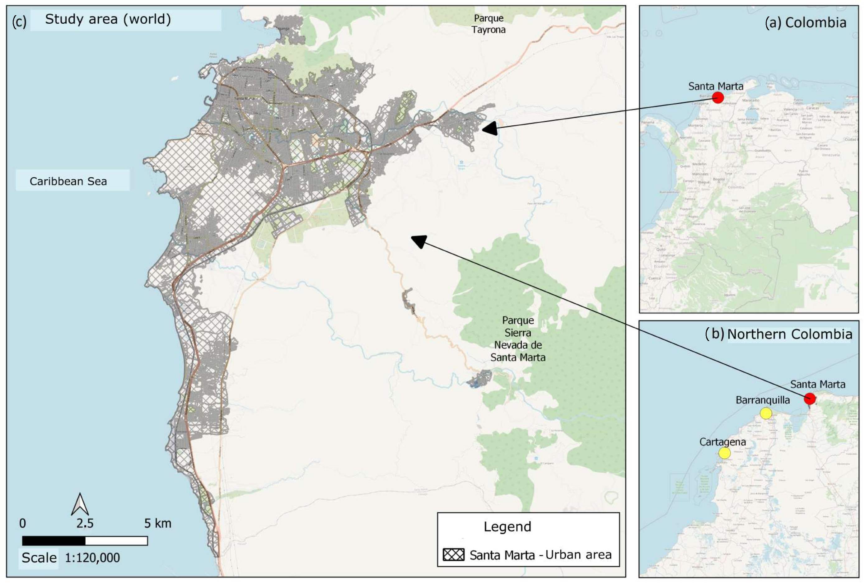
Entities are grouped into three groups: global environment (world), spatial units, and agents. The global environment is the spatial limit of the artificial world, geographically defined with a rectangle of 358 square kilometers (Km²); thus, it includes the urban area of Santa Marta and a populated center called Minca (see Figure 1). The state variables and parameters of the global environment are presented in

Table 1. State variables and parameters of the global environment.

Definition	Symbol 1	Code 2	Scale/Value
Parameters
Percentage of residents who move for recreation	$TR$	T_Recreo	[0–100]
Minimum speed at which agents move	$V_{min}$	min_speed	1 km/h
Maximum speed at which agents move	$V_{max}$	max_speed	60 km/h
Average speed at which agents move	$V_{media}$	prom_vel	30 km/h
Average size of agent groups that are recreated	$S_{media}$	Msize_group	3.786
State variables
Day and hour	T	starting_date	[1 January 2018–31 December 2018]
Hour	$T_h$	current_date.hour	[0–24]
Time in hours for each step	t	step	[1–760]
Minimum number of tourists in the world	$Mi{n}_{NT}$	MinTuristas	/
Maximum number of tourists in the world	$Ma{x}_{NT}$	MaxTuristas	/
Number of tourists daily in the world	$NT$	NTuristas	[$Mi{n}_{NT}$–$Ma{x}_{NT}$]

¹ Nomenclature used to identify variables in the paper. ² Nomenclature used to identify variables in the software used.

. The road network spatial unit is made up of lines and nodes through which agents move between blocks (manzanas, abbreviated as MZs), which represent the basic spatial unit of the model.

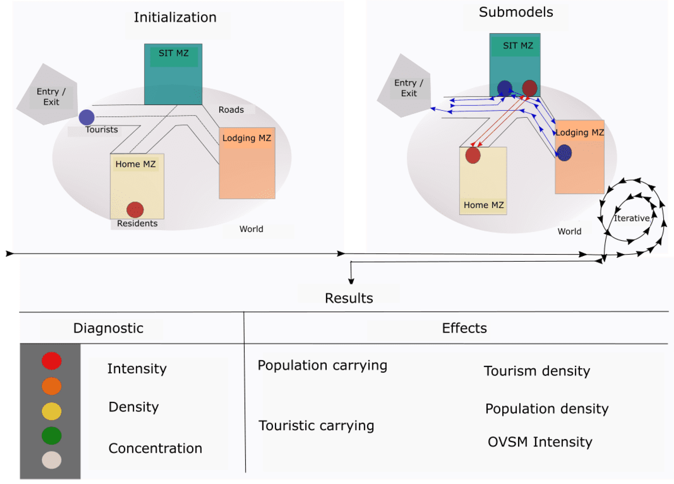
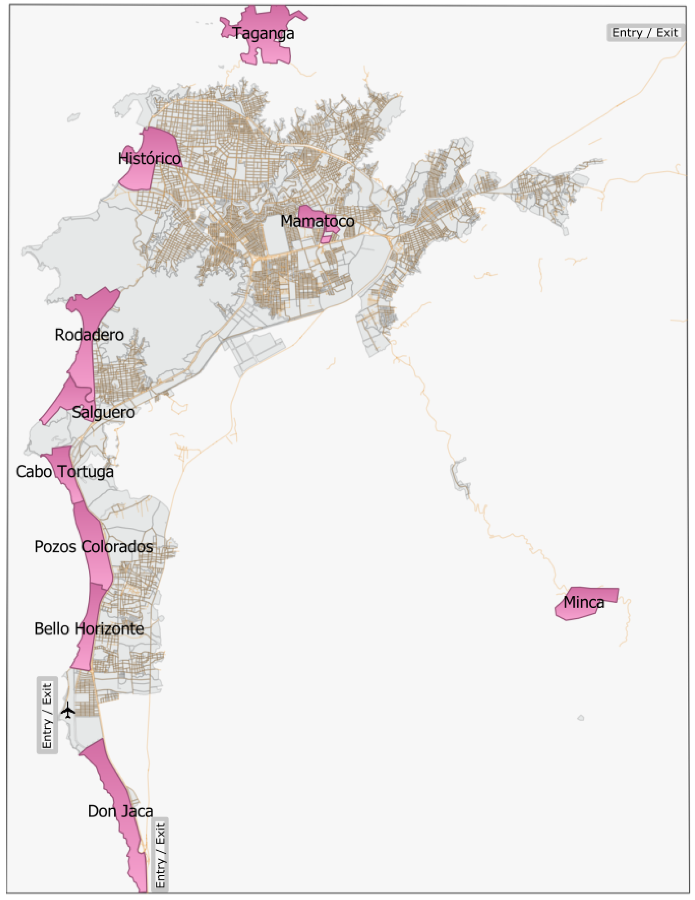
The block spatial units (MZs) represent polygons where agents carry out activities. The MZ can be places of residence (Home MZs), places of recreation (SIT MZs), and lodging places (Lodging MZs) (see Figure 2). MZ categories are not mutually exclusive, that is, the MZ can be of different types. The MZ are grouped by geographical zones of tourist interest (ZITs), a characterization developed in the POT (Zoning Land Plan) of Santa Marta of 2020 [40] (see Figure 3). The state variables and parameters of MZ are presented in

Table 2. State variables and parameters of the spatial blocks (MZs).

Definition	Symbol 1	Code 2	Scale/Value
Parameters
Minimum per-capita public space needed in SIT-MZ	$E{P}_{pc}$	espput_pc	15
State variables
Entry MZ: dichotomous variable indicating that the MZ is an entry for tourists to the destination	$IN$	INOUT	[0–1]
Lodging MZ: dichotomous variable indicating the presence of lodging in MZ	$HP$	LODGING	[0–1]
SIT MZ indicating the presence of tourist sites	$AT$	AT	[0–1]
SIT MZ with current tourist use	$UT$	UT	[0–1]
SIT MZ beach	$SI{T}_{playa}$	Playa	[0–1]
SIT MZ with cultural and historical heritage	$SI{T}_{pch}$	EPCH	[0–1]
SIT MZ with commercial center	$SI{T}_{com}$	Comercial	[0–1]
SIT MZ with parks	$SI{T}_{par}$	Parque	[0–1]
SIT MZ with natural site (excludes beach)	$SI{T}_{nat}$	SN	[0–1]
SIT MZ with public space	$EP$	EP	[0–1]
SIT MZ to identify Playa Rodadero	$SI{T}_{rod}$	ROD	[0–1]
SIT MZ to identify Playa Blanca	$SI{T}_{bc}$	PB	[0–1]
SIT MZ to identify Playa Bello Horizonte	$SI{T}_{BH}$	BH	[0–1]
SIT MZ to identify Playa Taganga	$SI{T}_{tag}$	TG	[0–1]
SIT MZ to identify Centro Histórico	$ZI{T}_{CH}$	CH	[0–1]
ZIT MZ to identify Rodadero	$ZI{T}_{RD}$	RD	[0–1]
ZIT MZ to identify Salguero	$ZI{T}_{SG}$	SG	[0–1]
ZIT MZ to identify Mamátoco	$ZI{T}_{MT}$	MT	[0–1]
ZIT MZ to identify Pozos Colorados	$ZI{T}_{PC}$	PC	[0–1]
ZIT MZ to identify Bello Horizonte	$ZI{T}_{BH}$	BEHO	[0–1]
ZIT MZ to identify Don Jaca	$ZI{T}_{DJ}$	DJ	[0–1]
ZIT MZ to identify Cabo Tortuga	$ZI{T}_{CT}$	Ct	[0–1]
ZIT MZ to identify Taganga	$ZI{T}_{TAGA}$	TAGA	[0–1]
ZIT MZ to identify Minca	$ZI{T}_{MC}$	MC	[0–1]
SIT MZ Top20: dichotomous variable that identifies the SIT that is one of the 20 most visited	$SI{T}_{t20}$	T20	[0–1]
SIT MZ Top5: dichotomous variable that identifies the SIT that is one of the 5 most visited	$SI{T}_{t5}$	T5	[0–1]
Residents	$R_m$	Personas	$[0-n(residents\left)\right]$
Residents who move for recreation	d	NR_REC	$[0-R_m]$
Block area (m2)	$A_m$	area	(0–5,886,274]

¹ Nomenclature used to identify variables in the paper. ² Nomenclature used to identify variables in the software used.

.

The residents are agents who permanently carry out activities within the destination: they live and recreate in the MZ, but in the model, they only move between MZs to carry out recreational activities in the MZ SIT and return to the home MZ through the highway network. Taking into account the results of the Population and Housing Census of Colombia 2018, the number of residents in the global environment is 453,527 people, distributed according to the results of the Census in the different MZs. The state variables and parameters of the residents are observed in

Table 3. State variables and parameters of residents.

Definition	Symbol 1	Code 2	Scale/Value
Parameters
Minimum hour to move for recreation	$HD{R}_{min}$	h_rec_start	7
Maximum hour of return to MZ home	$HD{R}_{max}$	h_rec_end	20
State variables
Velocity (RVTND) 3	$V_i$	speed	[$V_{min},V_{media},V_{max}$] 4
Home MZ	$M{Z}_i$	living_place	Home MZ startup
SIT MZ for recreation	$M{Z}_{SIT}$	SIT_placeD	Random selection
Target: string	$R_{obj}$	objective	[r, rec] 5
Localization	$lo{c}_i$	location	Coordinates
Hour to move for recreation (RV) 6	$HD{R}_i$	start_rec	[$HD{R}_{min}-(HD{R}_{max}-1)$]
Hour of return to MZ home (RV)	$HDR{F}_i$	end_rec	[$HD{R}_i-HD{R}_{max}$]
Size of the group of residents who move for recreation (RV)	$S_{t}r$	size_groupTR	[1–6]

¹ Nomenclature used to identify variables in the paper. ² Nomenclature used to identify variables in the software GAMA. ³ Random variable with truncated normal distribution. ⁴ [Lower limit, Average, Upper limit]. ⁵ [resting (r), recreating (rec)]. ⁶ Random variable.

.

Tourists are external agents that enter the system daily at various times. They are represented by travel groups of different sizes, and they enter the destination through an entry MZ, they carry out lodging or recreation activities in the MZ, and then they move through the road network. The state variables and parameters of the tourists are listed in

Table 4. State variables and parameters of tourists.

Definition	Symbol 1	Code 2	Scale/Value
Parameters
Minimum hour of entry to the destination	$H{T}_{min}$	min_in_start	5
Minimum number of hours at the destination	$H{S}_{min}$	Min_HstaySM	4
Maximum number of days at destination	$D{S}_{max}$	Max_DstaySM	15
Minimum hour to enter at the lodging	$Hi{n}_{min}$	Min_Hlodging	18
Maximum hour to enter at the lodging	$Hi{n}_{max}$	Max_Hlodging	23
Minimum departure time for overnight tourists to the attractions	$HN{D}_{min}$	Min_Hndrecreation	6
Maximum departure time for overnight tourists to the attractions	$HN{D}_{max}$	Max_Hndrecreation	10
State variables
Average days at the destination	$\widehat{D}$	P_DstaySM	[3.7–6.2]
Velocity (RVTND) 3	$V_i$	speed	[$V_{min},V_{media},V_{max}$] 4
Destination input and output MZ	$M{Z}_{inout}$	IN_place	Random selection
Lodging MZ	$M{Z}_l$	lodging_place	Random selection
SIT MZ to visit	$SIT$	SIT_place	Random selection.
Target: string	$T_{obj}$	objective	[r, l, n, g, b] 5
Localization	$lo{c}_i$	location	Coordinates
Hour of stay in Santa Marta (RVTND${)}^3$	$H_{stay}$	hstaySM	[$H{S}_{min},\widehat{D}\ast 24,D{S}_{max}\ast 24$]
Hour of entry to the lodging (RV) 6	$Hi{n}_{hos}$	hinlodging	[$Hi{n}_{min}$–$Hi{n}_{max}$]
Hour of move from entry MZ to SIT MZ (RV)	$H{T}_{in}$	startin	[$H{T}_{min}$–$Hi{n}_{hos}$]
Departure hour of tourists who spend the night at SIT MZ (RV)	$HND$	hnd_recreation	[$HN{D}_{min}$–$HN{D}_{max}$]
Travel group size	S	size_group	[1–10]

¹ Nomenclature used to identify variables in the paper. ² software code GAMA. ³ Random variable with truncated normal distribution. ⁴ [Lower limit, Average, Upper limit]. ⁵ [recreation (r), lodging (l), ndrecreation (n), goout (g), bye (b)]. ⁶ Random variable.

.

The model proceeds with time intervals of one hour (step) (t); its start date is 1 January 2018 at 00:00 h. All entities initialize with related attributes in state variables and parameters. Agents are shown on the map with circles representing the travel group size. Residents are shown in red circles, who are initially located in the home MZ. There is a percentage of residents who move for recreation ($TR$) and that determines the resident population that will move for recreation. Tourists are shown by blue circles, who initialize at the entry MZ. There is a minimum ($V_{min}$), maximum ($V_{max}$), and average ($V_{media}$) speed for agents to move within the destination, where all agents randomly select the speed at which they expect to move within the world, taking into account the speed parameters mentioned. There is a road network that joins the MZs, through which the agents will move (see initialization in Figure 2).

Consecutively, agents move between MZs to accomplish different objectives. Tourists move to a SIT MZ; if they are willing to spend more than 24 h in the city, then, they will move to a lodging MZ at the time of entry to the lodging area; otherwise, they will move to the entry-exit MZ to leave the world, an action that is repeated every day. In each step, one hour is subtracted from the variable hours of stay in Santa Marta. When this counter reaches zero, it is the moment when the tourist leaves the world. Every day, new tourist agents are generated randomly, in an interval defined in the global environment state variable: a minimum number of tourists in the world (lower limit) and a maximum number of tourists in the world (upper limit). In the case of residents, only those who have recreation as their objective will move, and they will move to an MZ SIT at the time established for this activity for each agent, and afterward, they will return to the MZ Home at the established return time (see submodels in Figure 2).

The first result of the model assesses the presence of the phenomenon through the indicators: intensity, density, and concentration. In the effects, it is possible to know the population and tourist distribution into the destination, changes in the population density and the tourist density, and a novel proposed indicator of the tourism intensity ($I_{sm}$) (see results in Figure 2).

2.2. Details

The software used in the simulation was GAMA, which facilitates the use of geographic information and can handle numerous agents [41]. The global environment attributes, roads, city blocks (MZs), number of residents, and their location, are created from a geographic information system (GIS) file. The number of residents that will move for recreation depends on the percentage of residents who move for recreation ($TR$). This is a parameter that can be changed by the modeler; this research used 1%.

2.2.1. Input Data

For the world, the minimum and maximum speed parameters of the agents are proposed by the modeler, and they were set at 1 km/h and 60 km/h; the average speed is 30 km/h, according to empirical evidence estimated by Roda [42]. The number of tourists entering daily is randomly generated with a truncated normal distribution. The simulations recreate the conditions for the year 2018, and thus, the data of monthly arrivals by plane to the city of Santa Marta in 2018 were used as an empirical approximation (see Table 5). For the average size of the groups of agents who travel for recreation, the monthly average size of the travel group for the department of Magdalena in 2018, estimated by FONTUR [43], was used.

For the blocks (MZs), the most important spatial unit of the model, the input data were obtained from GIS files. The base layer is the Colombian Geostatistical Framework for the 2018 census of DANE [44]; this base provided census information on the number of residents for each MZ, and the MZ that has temporary housing. The Santa Marta Land Management Plan (2020–2032) generated a spatial category called zones of tourist interest (ZITs), which are spaces of importance for the city’s tourist activity. This information is an input for the model to select the MZ that are part of the ZIT. Geographic data were obtained from Fundación OpenStreetMap [45], and the variables obtained were: (1) MZ lodging (MZs with places of lodging), enriched with information from MZs that have temporary housing from DANE [44] and are located within a ZIT; (2) MZs with sites of tourist interest (SIT MZs) and associated attributes, enriched with the Magdalena Tourist Guide, prepared by MinCIT [46]; and (3) Santa Marta road network.

Table 5. Average monthly, daily, and interval arrivals by plane for Santa Marta. Source: data of monthly passengers air arrivals of AERONÁUTICA CIVIL [47].

Month	Monthly Passengers 1	Daily Average	Interval
January	78,512	2533	[2033–3033]
February	60,356	2156	[1656–2656]
March	70,624	2278	[1778–2778]
April	66,838	2221	[1721–2721]
May	66,590	2148	[1648–2648]
June	81,513	2717	[2217–3217]
July	87,065	2809	[2309–3309]
August	85,220	2749	[2249–3249]
September	80,779	2693	[2193–3193]
October	87,748	2831	[2331–3331]
November	103,864	3462	[2962–3962]
December	123,105	3971	[3471–4471]

¹ Refers to the average number of monthly air passengers arriving at Simón Bolívar International Airport.

Table 5. Average monthly, daily, and interval arrivals by plane for Santa Marta. Source: data of monthly passengers air arrivals of AERONÁUTICA CIVIL [47].

Month	Monthly Passengers 1	Daily Average	Interval
January	78,512	2533	[2033–3033]
February	60,356	2156	[1656–2656]
March	70,624	2278	[1778–2778]
April	66,838	2221	[1721–2721]
May	66,590	2148	[1648–2648]
June	81,513	2717	[2217–3217]
July	87,065	2809	[2309–3309]
August	85,220	2749	[2249–3249]
September	80,779	2693	[2193–3193]
October	87,748	2831	[2331–3331]
November	103,864	3462	[2962–3962]
December	123,105	3971	[3471–4471]

¹ Refers to the average number of monthly air passengers arriving at Simón Bolívar International Airport.

For the diagnostic indicators, the methodology proposed by WTTC and McKinsey & Company [15] was used, which uses information from Tripadvisor. This methodology classifies the 5 most visited MZs for the concentration indicator and the 20 most visited MZs for density. The classification of the MZs for the destination Santa Marta on 30 October 2020 is presented in

Table 6. List of the 20 most visited attractions. Source: modified from Tripadvisor [48], on 30 October 2020.

No.	Attraction	No.	Attraction
1	Playa Blanca	11	Parque Simón Bolívar
2	Parque de los Novios	12	Iglesia San Francisco de Asís
3	Quinta de San Pedro Alejandrino	13	Marina de Santa Marta
4	Playa El Rodadero	14	Centro Comercial Arrecife
5	Catedral de Santa Marta	15	Reserva Natural Mamancana
6	Acuario del Rodadero	16	Centro Comercial Zazue
7	Estatua del Pibe	17	Playa de Bello Horizonte
8	Museo del Oro Tayrona	18	Centro Comercial Buenavista
9	Mundo Marino	19	Centro Comercial Ocean Mall
10	Camellón Rodrigo de Bástidas	20	Playa Bahía de Santa Marta

.

The residents get the input location data from the home MZs. Taking into account the global parameters, the following are randomly selected: the size of the recreation group, the mobilization time to leave for the SIT MZ and return home, and the mobilization speed of each resident who moves for recreation.

The tourists start in the world in an entry MZ. There are three MZs: the highway entrance from the south, on the road that connects with the municipality of Ciénaga; the entrance from Simón Bolívar international airport; and the road entrance from the northeast, by the road that connects with Tayrona Park (see Figure 3).

Data from empirical observations for the Department of Magdalena of FONTUR [43] were used: (1) average length of stay, which is measured in nights and does not include people who do not stay overnight and (2) the average size of the travel group. The average value of the data are presented as a continuous variable, but the variable size of the group used in this model is a discrete variable, so, for its use, a possible distribution was generated with an average equal to the size of the travel group provided by FONTUR [43].

The selection of the SIT MZs to visit arises from a random process; however, they have a different probability of being visited, since the evidence shows that some sites are more visited than others. For the assignment of probabilities, information published by FONTUR [43] was used, on the activities carried out by the visitor in Magdalena for the year 2018, which includes, among others: visits to beaches; visits to museums, houses of culture, churches, and monuments; visits to natural parks, waterfalls, rivers, wells, spas, zoos, and botanical gardens; sports practice; visits to discos, bars, karaoke, and dance floors; and walks along the streets and in parks of the urban area. Taking into account the objectives of this research and the tourist activities carried out, the activities were regrouped into beaches, cultural and historical sites, shopping centers, natural sites (excluding beaches), and parks, to which the average, as presented by FONTUR [43], was assigned (see

Table 7. Probability of visit for sites of tourist interest (SITs) in Santa Marta. Source: information elaborated with data taken from FONTUR [43], Redacción CV Noticias [49], Hoy Diario del Magdalena [50], El Informador [51], Montoya [52], and Iguaran [53].

SIT	SIT	Probability
Beaches (82%)	Rodadero	48%
	Blanca	10%
	Bello Horizonte	4%
	Taganga	5%
	Others	15%
Cultural and historical sites		8%
Shopping centers		1%
Natural sites		7%
Parks		2%

).

Another important piece of evidence to highlight in the model is that the beaches have considerable differences in terms of the number of visits received, for example, El Rodadero beach is considered the most visited. However, there is no robust information system in the city for the collection, communication, and validation of information from the sector. In this way, a qualitative approximation of visit probabilities was built, taking into account the communications made by the local news media about the movement of tourists in high season and the distribution on the most important beaches (see Table 7).

2.2.2. Submodels

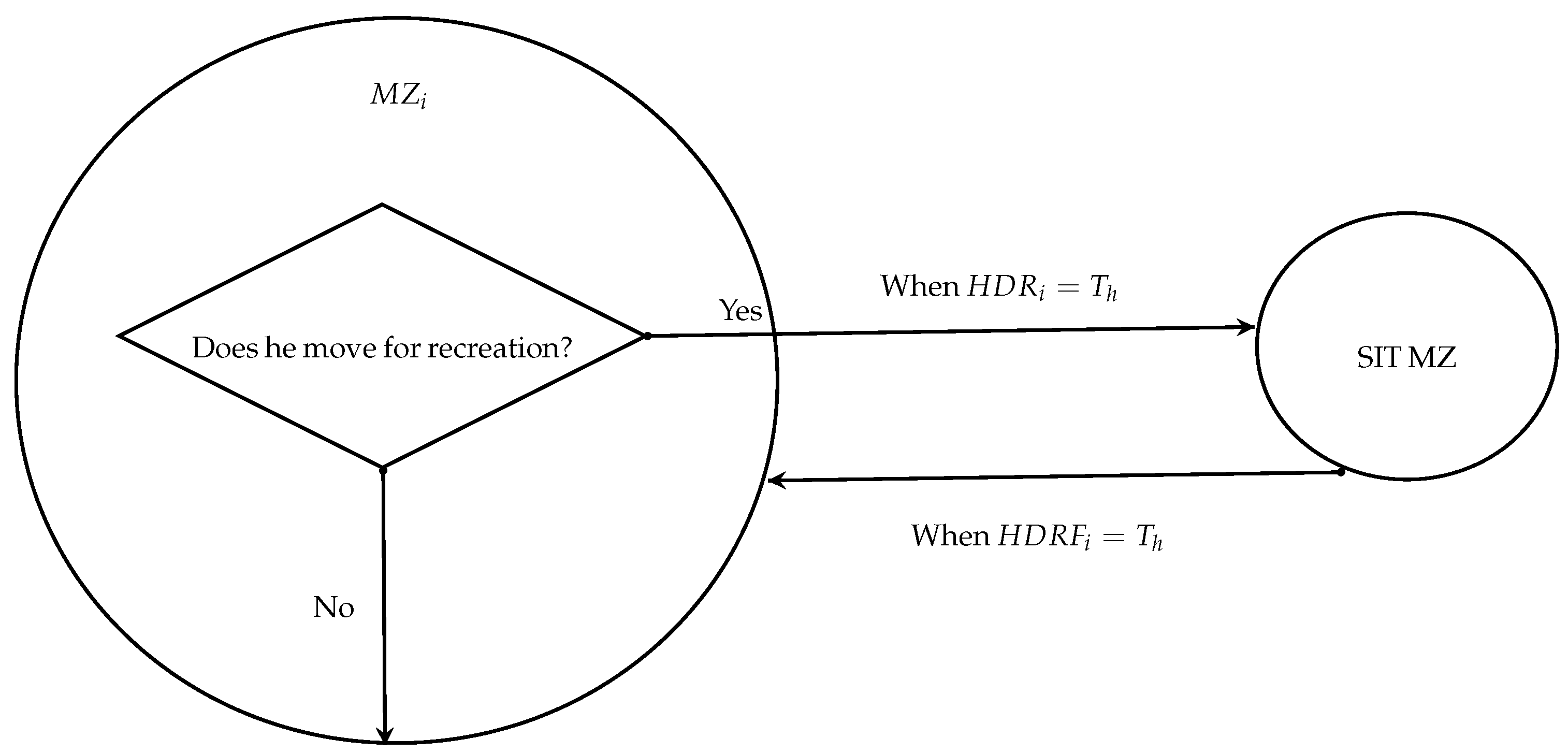
The residents have a home MZ ($M{Z}_i$); those who move for recreation randomly select a recreation SIT MZ ($M{Z}_{SIT}$), travel to that destination in one hour ($HD{R}_i$), and have one hour to return to their residence ($HDR{F}_i$). The residents have an objective ($R_{obj}$), which indicates the activity they are doing. This can be: resting (when they are in the residence) or recreating (when they are in the recreation SIT). In summary, the residents, considering their objective and the time ($T_h$), move or not, at the times established for each activity. It is important to mention that residents who move for recreation travel in groups of size S (see Figure 4).

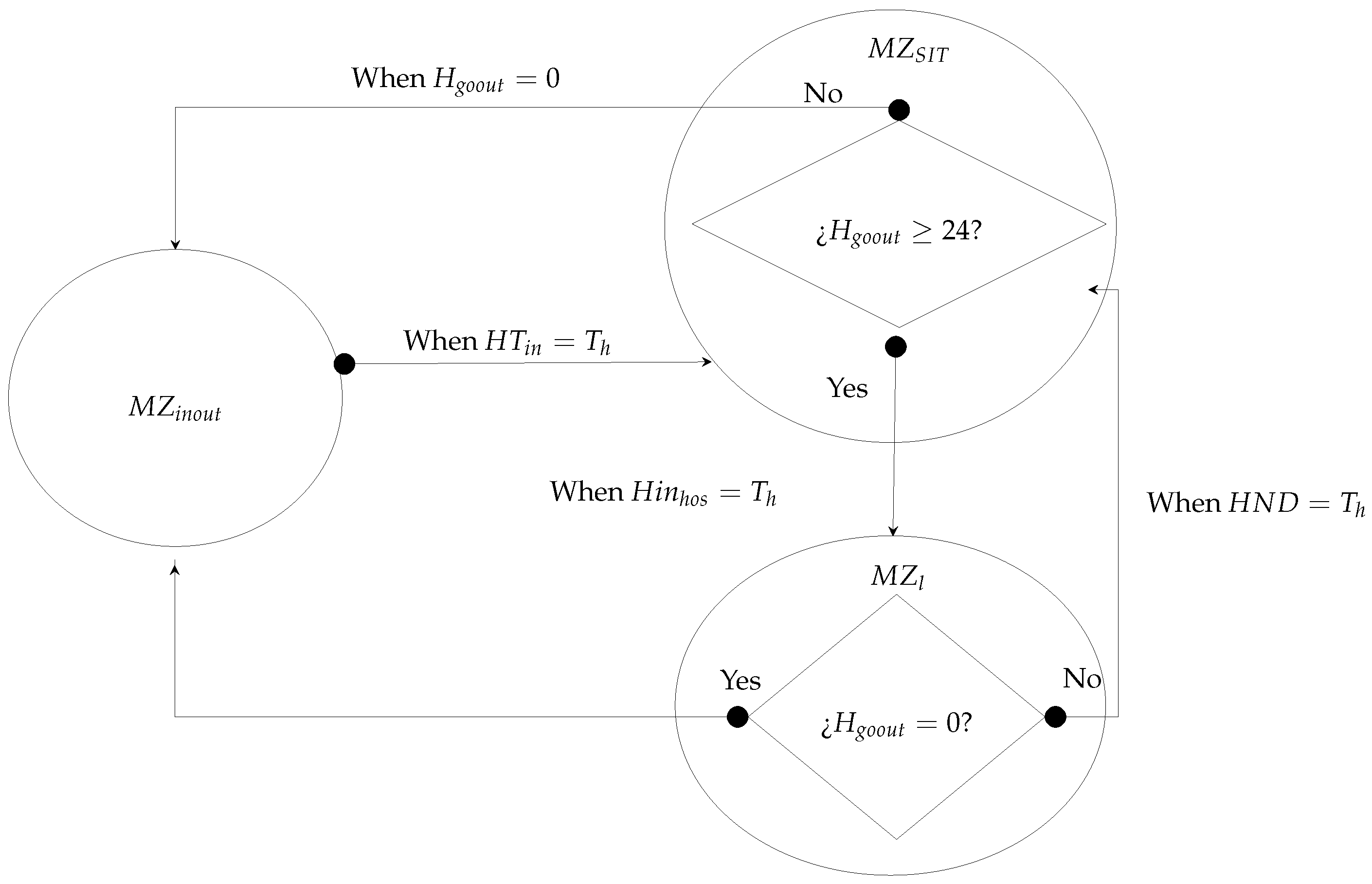
For their part, tourists enter Santa Marta for one MZ of entry ($M{Z}_{inout}$), and they move in groups of different sizes ($S_{tr}$) to the MZ-SIT to visit ($M{Z}_{SIT}$) at a given hour ($H{T}_{in}$). They have a duration at the destination ($H_{goout}$): if $H_{goout}\ge 24$, then the tourist spends the night in a lodging MZ ($M{Z}_l$) which the tourist enters at a certain time ($Hi{n}_{hos}$). However, if $H_{goout}<24$, then the tourist travels to $M{Z}_{inout}$ when $H_{goout}=0$. The overnight tourist evaluates the remaining hours in the destination ($H_{goout}$); if $H_{goout}=0$, then, they move to $M{Z}_{inout}$. Otherwise, they move to an $M{Z}_{SIT}$ at the determined time ($HND$) (see Figure 5).

2.3. Metrics

Peeters et al. [8] elaborated two indicators: tourism intensity (Intensity_pt), which is the ratio between the number of lodging nights and the number of residents, and tourism density (Density_pt), which is the ratio between the number of lodging nights and the destination area. WTTC and McKinsey & Company [15] elaborated three indicators: tourism intensity (Intensity_wt), which is the ratio between the number of tourists and the number of residents; tourism density (Density_wt), which is the ratio between the number of tourists and the area of the 20 attractions with the most visit (see Table 6); and tourism concentration (Concentration_wt), which is the ratio between the number of tourists to attractions in the top 5 of the destination (see Table 6) and the number of tourists in the destination. The diagnostic indicators in this research were elaborated through these three metrics; the algorithms are presented in

Table 8. Metrics and diagnostic inputs of overtourism.

Metric	Symbol	Algorithm
Tourists_fi	$x_t$	Tourists generated in each period
Tourists_Fi	$X_t$	${\sum }_{t=0}^{8760}{x}_t$
Tourists_fi5	$x_{5t}$	Tourist visits to attractions in the top 5
Tourists_Fi5	$X_{5t}$	${\sum }_{t=0}^{8760}{x}_{5t}$
Residents_Fi	${\mathbb{Y}}_t$	453,527
Lodging nights	$X{H}_t$	Add the nights of lodging of tourist
Area (km2) of the 20 attractions with the most visits	$A_{i20}$	0.597119
Destination area (km2)	$A_I$	358
Intensity_wt	$I_{wt}$	$X_t/{\mathbb{Y}}_t$
Intensity_pt	$I_{pt}$	$X{H}_t/{\mathbb{Y}}_t$
Density_wt	$D_{wt}$	$X_t/A_{i20}$
Density_pt	$D_{pt}$	$X{H}_t/A_I$
Concentration_wt	$C_{wt}$	$X_{5t}/X_t\ast 100$

.

In order to identify a situation of overtourism, the scales by quintiles generated by WTTC and McKinsey & Company [15] and Peeters et al. [8] were used, which identify destinations with a high risk of overtourism as those who are in first quintile ($Q_1$), while the location in higher quintiles indicates a lower risk of the presence of the phenomenon. To facilitate the communication of the diagnostic indicators, the values were reassigned as follows: the values of $Q_1$ indicate the lowest risk; consecutively, the values of $Q_5$ indicate a high risk. In the same way, colors are assigned in the next figures from facilitate identification, thus beige for $Q_1$, green for $Q_2$, yellow for $Q_3$, orange for $Q_4$, and red for $Q_5$ (see

Table 9. Diagnostic indicators and identification scales.

${\mathit{Q}}_{\mathit{i}}$	Intensity		Density		Concentration
	${\mathit{w}}_{\mathit{t}}$	${\mathit{p}}_{\mathit{t}}$	${\mathit{w}}_{\mathit{t}}$	${\mathit{p}}_{\mathit{t}}$	${\mathit{w}}_{\mathit{t}}$
$Q_5$	$I{w}_t>5.3$	$I{p}_t>9.6$	$D{w}_t>$ 930,000	$D{p}_t>$ 2278	$C{w}_t>36$
$Q_4$	2.8 $<I{w}_t\le 5.3$	$6.3<I{p}_t\le 9.6$	475,000 $<D{w}_t\le$ 930,000	1174 $<D{p}_t\le$ 2278	$33<C{w}_t\le 36$
$Q_3$	$1.8<I{w}_t\le 2.8$	$4.5<I{p}_t\le 6.3$	200,000 $<D{w}_t\le$ 475,000	$719<D{p}_t\le$ 1174	$29<C{w}_t\le 33$
$Q_2$	$1.0<I{w}_t\le 1.8$	$3.2<I{p}_t\le 4.5$	75,000 $<D{w}_t\le$ 200,000	$407<D{p}_t\le 719$	$22>C{w}_t\le 29$
$Q_1$	$I{w}_t\le 1$	$I{p}_t\le 3.2$	$D{w}_t\le$ 75,000	$D{p}_t\le 407$	$C{w}_t\le 22$

and Figure 2).

For the measurement of effects, the population carrying ($C_t$) was estimated, where it is the addition of the resident and floating population that uses the territory [54]. For the residents, we used the size of the resident population ${\mathbb{Y}}_t$; and for the floating population, the number of tourists in a period ${\mathbb{X}}_t$ can be expressed as:

$$C_t={\mathbb{Y}}_t+{\mathbb{X}}_t$$

(1)

Taking into account the problem of oversizing tourism carrying, the ABM of urban overtourism in Santa Marta allowed to propose an indicator of the relationship between the floating tourist population and residents, which seeks to know the intensity of tourism, should take into account that while residents use the territory all year round, tourists do so at much shorter intervals. The research can generate an intensity indicator, where the resident population is included in using the territory all day, and the floating tourist population uses the territory for the segment of time that it is in the destination. Thus, to generate an analogous measurement unit between the flow of tourists and residents, the calculation of the person-years lived ($PYL$) added by tourists is proposed, which means adding only the time that the tourist is in the urban destination. For example, for a tourist who visits the destination for 10 days, the $PYL$ that they add is a fraction of the year equal to $10/365$. Thus, when there are no tourists, the population carrying is a value equal to the resident population; with the presence of tourism, tourists add the sum of the parts of the day that they use the territory, that is, their $PYL$. This concept of $PYL$ is used for the construction of mortality tables and the calculation of life expectancy in demography [55].

The person-years lived ($PYL$) added by tourists in the destination are estimated, which corresponds to the time measured in years that tourists remain in the city. The sum of the $PYL$ allows for estimating the tourist carrying (${\mathbb{X}}_t$). For the population carrying of residents, the population carrying corresponds to the population of the destination in the year (${\mathbb{Y}}_t$). The proposed tourism intensity indicator, called the Santa Marta Overtourism Intensity ($I_{sm}$), is calculated as the ratio between the population carrying added by tourists and the population carrying of residents. It can be expressed as:

$$I_{sm}={\displaystyle \frac{{\sum }_{t=0}^{8760}PYL}{{\mathbb{Y}}_t}}={\displaystyle \frac{{\mathbb{X}}_t}{{\mathbb{Y}}_t}}$$

(2)

Finally, with the sum of the population carrying that adds the $PYL$ of tourists and residents, the population carrying $C_t$ is estimated taking into account Equation (1). From the model, t is the step that is 8760 h of the year.

2.4. Scenarios

This research analyzes the results of the application of two management measures. The measures were selected because they are plausible measures in the short term (one year) and observable with the parameters and variables of this model. None of the measures make changes in the number of tourists that enter the urban system, since it is an undesirable measure for the actors of the tourism sector and difficult to apply; in this sense, the measures only have an effect on the spatial and temporal distribution of visitors within the destination. The two management measures evaluated are:

• ($M_1$) Increase in the number of SIT MZ that have tourist use. It consists of increasing the tourist attractions that have tourist use, incorporating those proposed in the Magdalena Tourist Guide MinCIT [46]. In practice, this measure can be implemented through knowledge management of the city’s attractions. The proposed tourist attractions are listed in

  Table 10. List of new attractions.

  Attraction	Attraction
  Polideportivo	Centro Comercial la 22
  Morro	Playa del amor
  Playa Lipe	Punta Betín
  Playa Santo Cristo	Centro Comercial Plazuela 23
  Gobernación	Palacio de Justicia
  Parque Sesquicentenario	Hospital San Juan de Dios
  Centro Comercial las Olas	Centro Comercial la 22
  Alcaldía	Centro Cultural San Juan Nepomuceno
  Casa de Don Joaquín de Mier	Casa Campo Serrano
  Casa Alzamora	Centro Comercial Santa Marta Aquarium
  Parque de la Iglesia de Taganga	Concejo municipal
  Fuerte de San Fernando	Casa del Marqués
  Casa Madame Agustín	Casa Noguera

  .
• ($M_2$) Communication in real time of the level of agglomeration of the sites of tourist interest. It consists of informing the agents (tourists and residents) about the level of agglomeration of the MZ SIT to visit; then, with this information, the agents can change the decision of the place to visit, in this case, if ${\displaystyle \frac{m^2}{person}}<15$ in the MZ to visit, then, they change their decision to visit a place with a value greater than or equal to 15. The minimum public space proposed in DNP [56] was assumed. In practice, this measure can be implemented through a mobile application, where the agent receives information on the level of agglomeration in real time.

Then, four scenarios are proposed: without measures ($E_0$), with $M_1$ for $E_1$, with $M_2$ for $E_2$, and the combination of $M_1$ and $M_2$ for $E_3$.

3. Results

Forty simulations were generated for the analysis of overtourism, with ten experiments for each $E_i$. In all the simulations, a maximum of 1,194,110 annual tourists and a minimum of 1,159,402 were generated (see

Table 11. Results of experiments in $E_i$ for Santa Marta for a year.

${\mathit{E}}_{\mathit{i}}$	${\mathit{X}}_{\mathit{t}}$1	${\mathit{I}}_{\mathit{wt}}$	${\mathit{I}}_{\mathit{pt}}$	${\mathit{D}}_{\mathit{wt}}$	${\mathit{D}}_{\mathit{pt}}$	${\mathit{C}}_{\mathit{wt}}$	${\mathbb{X}}_{\mathit{t}}$2	${\mathit{C}}_{\mathit{t}}$3	${\mathit{I}}_{\mathit{sm}}$
$E_0$	1,166,480	2.572	10.722	1,953,512	13,581	36.671	15,635	469,162	0.034
$E_0$	1,172,034	2.584	10.803	1,962,813	13,683	36.594	15,701	469,228	0.035
$E_0$	1,173,196	2.587	10.786	1,964,759	13,662	36.564	15,723	469,250	0.035
$E_0$	1,174,345	2.589	10.779	1,966,683	13,652	36.619	15,714	469,241	0.035
$E_0$	1,174,463	2.590	10.777	1,966,881	13,650	36.711	15,707	469,234	0.035
$E_0$	1,175,124	2.591	10.798	1,967,998	13,677	36.593	15,719	469,246	0.035
$E_0$	1,175,457	2.592	10.812	1,968,546	13,694	36.655	15,740	469,267	0.035
$E_0$	1,177,905	2.597	10.805	1,972,645	13,686	36.602	15,744	469,271	0.035
$E_0$	1,181,093	2.604	10.792	1,977,984	13,669	36.614	15,811	469,338	0.035
$E_0$	1,182,358	2.607	10.870	1,980,103	13,768	36.598	15,838	469,365	0.035
$E_1$	1,159,402	2.556	10.664	1,941,658	13,507	34.073	15,549	469,076	0.034
$E_1$	1,163,846	2.566	10.700	1,949,101	13,552	35.194	15,583	469,110	0.034
$E_1$	1,163,995	2.567	10.695	1,949,350	13,546	34.046	15,574	469,101	0.034
$E_1$	1,170,480	2.581	10.723	1,960,211	13,582	34.095	15,617	469,144	0.034
$E_1$	1,171,686	2.583	10.770	1,962,230	13,642	33.985	15,692	469,219	0.035
$E_1$	1,172,321	2.585	10.779	1,963,294	13,652	34.092	15,694	469,221	0.035
$E_1$	1,175,003	2.591	10.803	1,967,785	13,684	34.071	15,737	469,264	0.035
$E_1$	1,175,179	2.591	10.788	1,968,080	13,664	35.206	15,723	469,250	0.035
$E_1$	1,176,239	2.594	10.746	1,969,855	13,611	34,031	15,759	469,286	0.035
$E_1$	1,178,475	2.598	10.769	1,973,600	13,640	34.057	15,774	469,301	0.035
$E_2$	1,164,660	2.568	10.709	1,950,464	13,564	37.436	15,587	469,114	0.034
$E_2$	1,166,079	2.571	10.683	1,952,840	13,531	37.321	15,559	469,086	0.034
$E_2$	1,168,870	2.577	10.711	1,957,814	13,566	35.233	15,682	469,209	0.035
$E_2$	1,170,028	2.580	10.683	1,959,454	13,532	34.558	15,668	469,195	0.035
$E_2$	1,172,996	2.586	10.749	1,964,374	13,615	46.730	15,675	469,202	0.035
$E_2$	1,177,839	2.597	10.816	1,972,535	13,700	41.330	15,758	469,285	0.035
$E_2$	1,178,374	2.598	10.831	1,973,431	13,719	42.108	15,776	469,303	0.035
$E_2$	1,179,939	2.602	10.824	1,976,052	13,710	38.482	15,785	469,312	0.035
$E_2$	1,180,409	2.603	10.806	1,976,839	13,687	46.695	15,814	469,341	0.035
$E_2$	1,186,091	2.615	10.893	1,986,355	13,797	35.256	15,879	469,406	0.035
$E_3$	1,164,408	2.567	10.647	1,950,042	13,485	35.533	15,566	469,093	0.034
$E_3$	1,165,968	2.571	10.723	1,952,654	13,582	36.164	15,606	469,133	0.034
$E_3$	1,168,650	2.577	10.694	1,957,146	13,545	33.525	15,661	469,188	0.035
$E_3$	1,169,873	2.580	10.736	1,959,194	13,598	49.557	15,641	469,168	0.034
$E_3$	1,173,237	2.587	10.773	1,964,828	13,645	41.913	15,702	469,229	0.035
$E_3$	1,175,764	2.592	10.798	1,969,060	13,677	34.888	15,736	469,263	0.035
$E_3$	1,175,804	2.593	10.761	1,969,127	13,630	46.158	15,749	469,276	0.035
$E_3$	1,178,673	2.599	10.804	1,973,932	13,684	33.802	15,789	469,316	0.035
$E_3$	1,184,178	2.611	10.822	1,983,151	13,708	39.822	15,862	469,389	0.035
$E_3$	1,194,110	2.633	10.949	1,999,784	13,869	49.708	16,025	469,552	0.035

¹ Number of visitors to the destinations. ² Tourist carrying. ³ Population carrying.

). The color scheme is based on the quintiles of the tourism risk indicator (see Table 9), where yellow represents values in the third quintile, orange corresponds to the fourth quintile, and red indicates the highest risk in the fifth quintile. The value of $X_t$ varies across each scenario, as the number of daily tourists differs in every simulation. This variation results from a randomization process based on the data presented in Table 5.

3.1. Initial Scenario $E_0$

The diagnostic indicators show that under the conditions established in the model, there was a high risk of overtourism in all the simulations: the indicators $I_{pt}$, $D_{wt}$, $D_{pt}$, and $C_{wt}$ are in the $Q_5$, while $I_{wt}$ was located in $Q_3$ (see Table 11).

The model allows us to observe the moment when the diagnostic indicators are exceeded. Observing the moments of exceeding the diagnostic indicator is interesting for the analysis, since it shows that the indicators present different temporal scales of interpretation of the phenomenon. In addition, it can be used to measure the size of the effect; for example, from the first three months, there are already signs of a considerable increase in density. It is important to remember that the beginning of the count of the flows related to the study begins chronologically on 1 January and ends on 31 December.

The $I_{wt}$ is generally used to identify the pressures of tourism in a destination. For this research, a value above $2.5$ was estimated in all the experiments. Classically, this is interpreted as indicating that the population of tourists was 2.5 times above the residents. For its part, the $I_{sm}$ is a more adjusted indicator, since it only takes into account the part of the time that the tourist spent at the destination. Thus, it was estimated that tourists add a total person-year lived ($PYL$), which corresponds to the tourist carrying (${\mathbb{X}}_t$) received by the system, with a range between 15,635 and 15,838, which corresponds to a $I_{sm}=0.035$. These results are very important because they indicate that the city has a population growth of $3.5\%$ per year due to the floating population of tourists. The $I_{sm}$ presents considerably high values; if we take into account that in the population projections of DANE [44], the annual growth rate between 2005 and 2020 in the municipal seat of Santa Marta was around $1.74\%$. In other words, the growth of the tourist carrying can double the growth of the population carrying of residents (see Table 11).

The density of tourists excludes residents for the calculation, that is, it corresponds to the ratio between tourist visitors to the ZIT and its area. It shows the differences between ZITs (see

Table 12. Annual average tourist density per ZIT.

ZIT	Average Tourist Density
Rodadero	2,529,264
Minca	892,463
Bello Horizonte	488,606
Taganga	252,466
Centro Histórico	251,276
Cabo Tortuga	124,929
Mamatoco	103,403
Salguero	53,958
Don Jaca	23,156
Pozos Colorados	6454

). If we relate the values of the population density and the density of tourists by ZIT, it is evident that Rodadero and Minca are highly influenced by the growth in the number of residents and tourists. The Centro Histórico maintains high population densities as a result of the population residing in the area, and it is less influenced by tourism. At the other extreme, we have the case of Pozos Colorados, which has a low population density with a low density of tourism, indicating that it is an area of low intensity of use by residents and tourists (see Table 12).

At the MZ scale, we will analyze the changes in population density. The results are presented with a map of the city of Santa Marta, which was divided into three sections that allow observing the dynamics on a smaller spatial scale: the northern section includes Taganga, Centro Histórico, and Mamatoco; the central section includes Rodadero; and the southern section includes Cabo Tortuga, Pozos Colorados, Bello Horizonte, Don Jaca, and Minca. Similarly, there are four moments in the city: 8:00 a.m., 12:00 p.m., 4:00 p.m., and 10:00 p.m. The results presented correspond to January 5, 2018. For the graphic representation, the rate of change in population density ($\delta DP$), calculated as $\delta DP={\displaystyle \frac{D{P}_{t=i}-D{P}_{t=0}}{D{P}_{t=0}}}$; if $\delta DP\le 1$, the color of the MZ is green; if $1<\delta DP\le 3$, the color of the MZ is yellow; if $3<\delta DP\le 100$, the color of the MZ is orange; and if $\delta DP>100$, the color of the MZ is red (see Figure 6, Figure 7 and Figure 8).

In summary, we observe that there is a general pattern where densities increase in tourist sites during daylight hours, but once tourists and residents return to places of lodging and residence, the other MZs increase the population density values.

3.2. Scenarios with Management Measures $E_i$

The simulations show a stability of the diagnostic indicators $I_{wt}$, $I_{pt}$, $D_{wt}$, and $D_{pt}$, that is, they maintain similar values in the different experiments. The results continue to show that the city of Santa Marta presents conditions of overtourism; in addition, by construction, the indicators have a direct relationship with the number of visits (see Table 11).

The measures proposed with the scenarios have a considerable effect on the concentration indicator ($C_{wt}$). Initially, we can observe that in some experiments, the concentration goes from $Q_5$ in $E_0$ to $Q_4$ in the respective $E_i$ (see Table 11).

Let us analyze the effect of the proposed measure in $E_1$, whose comparison will be made with $E_0$. In this case, the measure decreases concentration levels at the destination up to $Q_4$, which indicates that increasing the sites of tourist interest decreases the concentration, and in the same way, we can observe that within these two scenarios the relationship between the number of visits and $C_{wt}$ is low, which shows that the change in the scale of $C_{wt}$ is the result of the change of scenery (see Figure 9).

$E_2$ and $E_3$ present an interesting emerging behavior with respect to concentration, where the results show that the measure does not have a clear pattern of behavior with evidence of an effect of the measure $M_2$ and $M_3$ on $C_{wt}$; we have a low concentration with a low and high number of visits and a high concentration with intermediate levels in the number of visits. The lack of a clear relationship is linked to the fact that the concentration has a high dependence on the preferences of SIT places by the visitors; this parameter receives little influence in this measure (see Figure 9).

The tourist carrying received by the system (${\mathbb{X}}_t$) in all the experiments is in a range between 15,549 and 16,025, which corresponds to a range of $0.034\leqq I_{sm}\leqq 0.035$ (see Table 11). The density of tourists shows the changes in the pressures generated by tourism on the scale of the tourist interest zone (ZIT) in front of the proposed scenarios.

When comparing $E_2$ with $E_0$, it is observed that the measure causes a decrease in the average density of tourists in Minca and the Centro Histórico; on the contrary, in the rest of the ZITs, the average density of tourists increases. This is the result of the spatial reassignment of tourists from small tourist attractions located in the Centro Histórico and Minca to the rest of the sites in the destination (see Figure 10). When comparing $E_3$ with respect to $E_0$, it is observed that the measure causes a decrease in the average density of tourists in Minca and Rodadero; on the contrary, in the rest of the ZITs, the average density of tourist increases (see Figure 10).

4. Discussion

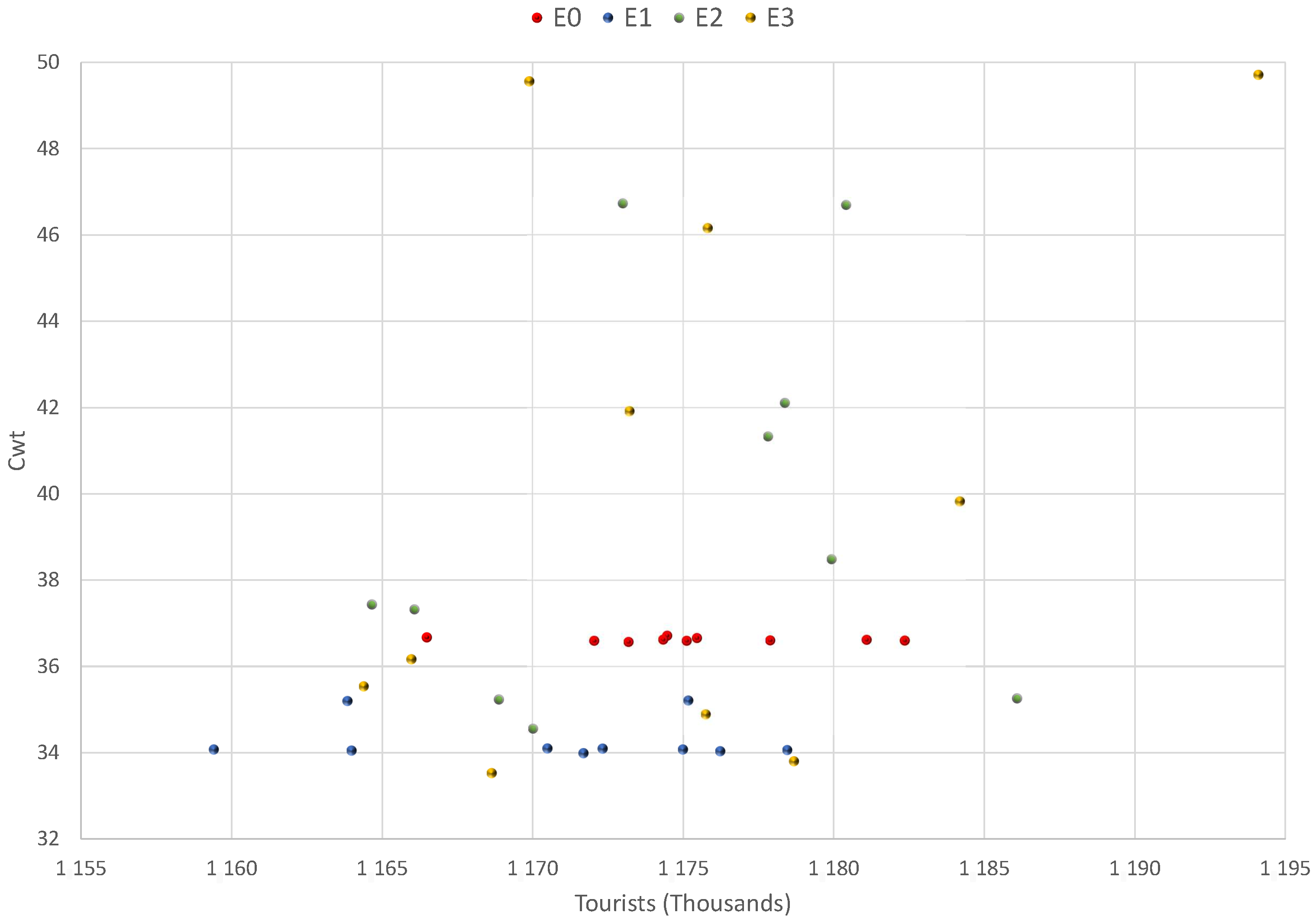
The ABM of overtourism in Santa Marta generated an important result, as it has the ability to generate a diagnostic of the presence of overtourism in this city. For the diagnostic indicators, stability was observed in all scenarios, where they remained in the same quintile, excluding the concentration indicator that showed greater volatility. This is the outcome of the indicator capturing the effect of the measures on the spatial and temporal distribution of the visits, which aims to highlight this indicator as an important metric for the analysis of overtourism.

Diagnostic indicators designed by Peeters et al. [8] and WTTC and McKinsey & Company [15] have analyzed aggregated and spatial scales of destiny. When compared with cities like Venice and Barcelona, two emblematic cases of overtourism, Santa Marta exhibits a high risk across most indicators. Specifically, its tourism density and intensity indicators surpass those of Barcelona, although they remain below those of Venice. Regarding tourism concentration, Santa Marta shows levels comparable to Barcelona but lower than Venice.

A key added value of this research lies in its ability to provide disaggregated spatial-temporal analysis, enabling the examination of tourism patterns not only at the city-wide level, but also across specific timeframes (from hourly to yearly) and localized areas such as individual tourist sites within Santa Marta.

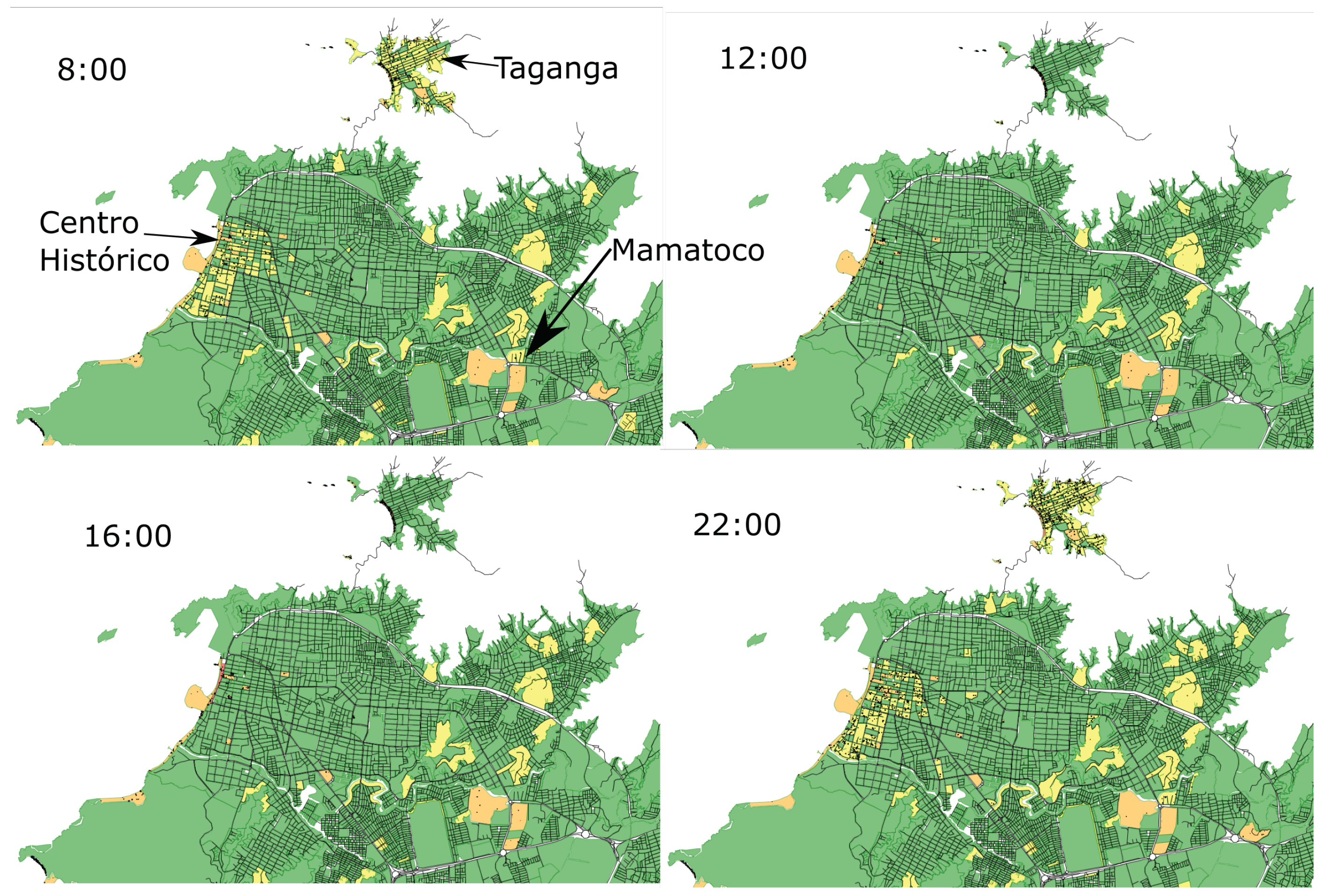
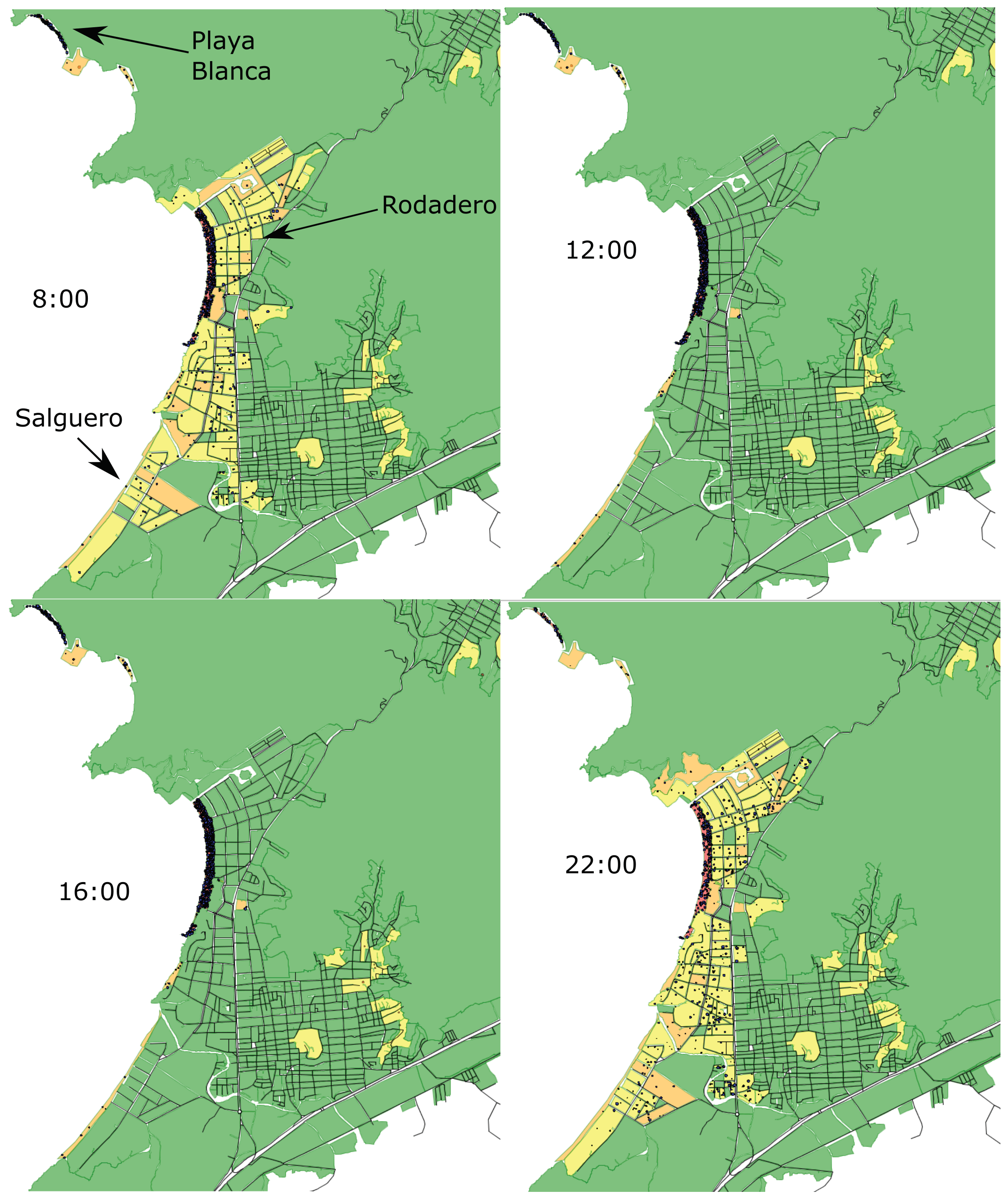
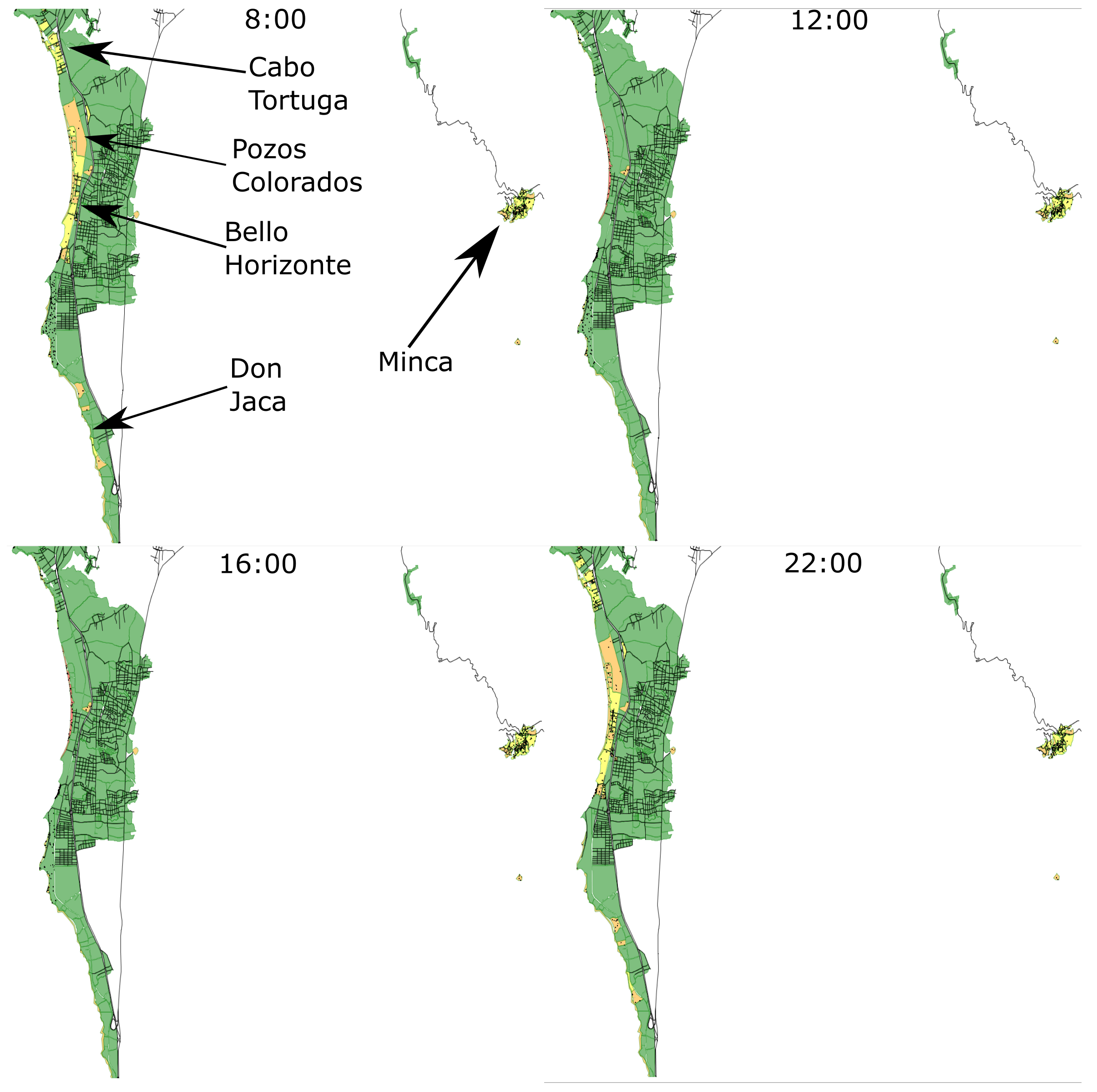
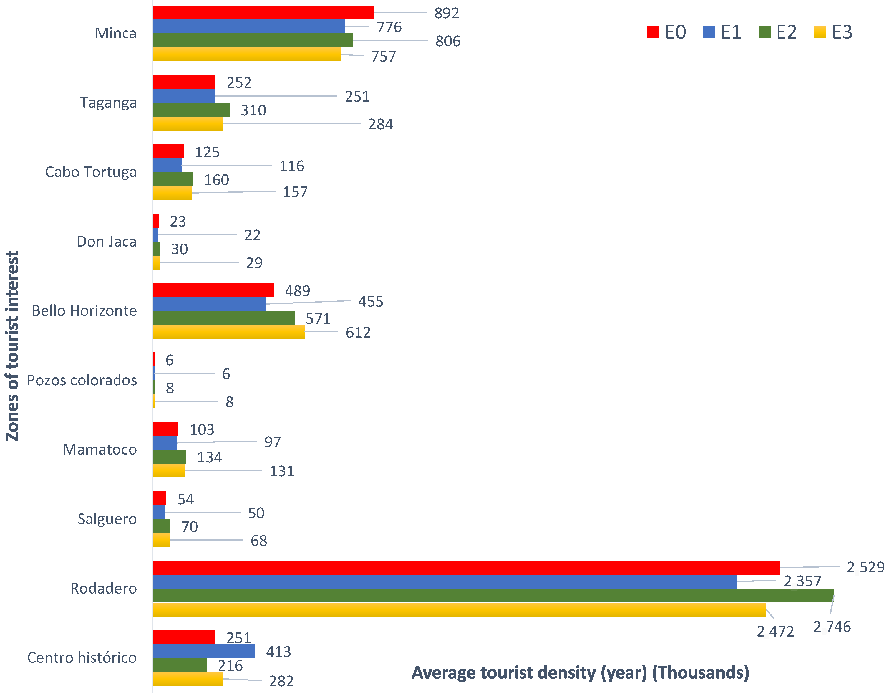
In the spatial scale, we have the ZITs where the population density has higher values in Rodadero, Centro Histórico, Minca, and Taganga; only $E_1$ generated a considerable increase in population density in the Centro Histórico. For its part, the density of tourists presented higher values in Rodadero, Minca, Bello Horizonte, Taganga, and the Centro Histórico, generating a differential effect between ZITs in the different scenarios. These results are important in terms of public policy goals associated with the spatial and temporal distribution of tourism in the city. For example, if the goal of reducing the number of tourists in Rodadero is proposed, then $E_1$ will achieve the goal objective; however, on the contrary, $E_2$ will increase the density of tourists, and with it, it will move us away from the proposed goal.

In addition to the main tourist zones, the model identified increases in tourist density in areas not traditionally associated with overtourism, such as Pozos Colorados and Mamatoco. Although these results may seem counterintuitive, they can be partially explained by underlying territorial dynamics. Pozos Colorados is characterized by its high scenic value and has undergone significant tourism-oriented development, including high-end hotels and recreational facilities that have driven up land values in recent years. Mamatoco, on the other hand, is located near important commercial centers, which may attract visitors indirectly. These findings suggest that tourism flows may extend beyond the classical zones of interest, highlighting the importance of analyzing peripheral urban dynamics in overtourism assessments.

In the temporal scales, the model allows observing temporal changes at a minimum scale (hours) and a maximum (year); likewise, it allows observing different spatial scales, from the minimum (MZ) to the maximum (destination). The minimum spatial and temporal scale allows observing changes in the MZ at various times of the day, that is, peaks of increase in population carrying can be observed in tourist sites in the hours of the day between 10:00 and 16:00, and subsequently, its decrease and increase in places of lodging and residence at night. This information may be relevant for the analysis of the effects of overtourism on smaller spatial and temporal scales.

These observations highlight the usefulness of spatial-temporal indicators to identify pressure zones and time-based dynamics in the destination. However, spatial metrics alone do not capture the full complexity of overtourism. While the model provides valuable insights into overtourism through spatial-temporal indicators such as density and intensity, it does not capture qualitative or perceptual dimensions of tourism pressures, including resident satisfaction, environmental degradation, or economic displacement. These experiential aspects are essential for a comprehensive understanding of overtourism. Future research should consider integrating qualitative methods—such as surveys, interviews, or environmental assessments—to complement the quantitative findings of agent-based simulations.

Additionally, the current model does not differentiate between tourist segments such as day-trippers, cruise tourists, or long-stay visitors. While this simplification was necessary due to data availability and computational constraints, we acknowledge that these groups exert different spatial and temporal pressures on destinations. Differentiating these profiles in future versions of the model could enhance its realism and support more targeted management strategies.

Regarding the proposed policy strategies, it is important to critically assess their feasibility in the local context of Santa Marta. While real-time crowd monitoring has shown potential in managing overtourism in highly digitized cities, its implementation in Santa Marta may be constrained by limited technological infrastructure, uneven internet connectivity, and institutional capacity. Nonetheless, low-cost and scalable alternatives—such as mobile-based reporting tools, signage systems, or coordination with tourism operators—could be viable first steps. These would require inter-institutional cooperation and gradual integration into local governance practices, which should be considered in any attempt to operationalize this strategy.

In terms of implementation and economic feasibility, the proposed strategies are intended as low-impact and adaptable interventions. The real-time crowd-monitoring strategy does not necessarily require sophisticated infrastructure but could be initiated through affordable pilot programs, such as SMS alerts, digital signage, or the use of existing public Wi-Fi data. Similarly, the diversification of tourist attractions refers not to costly construction projects, but to the activation and promotion of underutilized sites already recognized in local tourism plans. These approaches aim to optimize existing resources while fostering spatial dispersion and mitigating concentrated tourism pressure.

Although the model does not include direct stakeholder consultation, we recognize that the success of any tourism management strategy depends on the support and involvement of key actors. Residents may express concerns about increased tourism pressure resulting from the expansion of attractions, while local businesses could perceive crowd dispersion strategies as a potential threat to profitability in core areas. Conversely, local governments may view both strategies as tools to align tourism with urban sustainability goals. Future research should incorporate participatory approaches to assess stakeholder perceptions and foster collaborative decision making in the design of overtourism interventions.

It is also important to consider the potential unintended consequences of the proposed strategies. Expanding the number of tourist attractions may spatially redistribute visitor flows but not necessarily reduce the overall tourism pressure on the destination. Likewise, real-time crowd information may primarily benefit tourists with greater digital access or flexibility, potentially reinforcing existing inequalities. Budget travelers may continue to cluster in low-cost, high-density areas. These considerations highlight the need to accompany spatial dispersion strategies with inclusive communication tools and complementary measures that ensure equitable access and avoid shifting impacts from one vulnerable area to another.

5. Conclusions

In the context of overtourism studies, this research and the model used offer tools to illustrate the emerging dynamics of the interaction between agents and urban spaces, allowing that we have an interdisciplinary analysis that can be used to join urban and touristic sector studies; also, it can be used to simulate the possible results of management strategies. Finally, the model generates one new intensity indicator, the $I_{sm}$, which can be used to adjust the overestimation of classic intensity indicators of tourism.

Beyond its technical contributions, the model also presents opportunities for future expansion to address other important aspects of overtourism. It is important to note that this study focused primarily on quantifiable dimensions of overtourism. Although this allows for replicable, spatially disaggregated diagnostics, it does not account for subjective experiences or environmental impacts. Including qualitative data in future model, iterations would enhance the explanatory power of the model and support more holistic urban tourism management strategies.

The model can be used to estimate the tourist carrying capacity of the city; for this, it is necessary to generate more research on the relationship between visits and impact. However, if we assume that the moment when all the diagnostic indicators of overtourism are at $Q_5$, which is the moment when the carrying capacity is exceeded, then the results of this investigation allow us to estimate that Santa Marta has a tourist carrying capacity of 2,404,076 visits in a year for $E_0$.

However, the lack of robust statistical data presents a limitation for the model, as it restricts the ability to compare the ABM results with empirical patterns. Nevertheless, qualitative observations by Pupo [57] and [58] identify El Rodadero, Minca, Taganga, and the Historic Center as the areas with the highest tourism intensity—findings that align with the emergent spatial patterns produced by the model. This correspondence adds value to the model by supporting its potential to simulate the spatial-temporal distribution of tourism within the city.

As an instrument for measuring the observed and possible effects, the ABM model is a tool that allows evaluation of the path of development that the destination is following. Santa Marta is a city where the evolution of tourism began in the 1950s, and which is currently a destination in a state of maturity or consolidated on the national and international market. The diagnostic of overtourism of this research made it possible to show that the city presents a high-risk situation, and thus, the city is going through a moment of important inflection to determine its path of development, which from the perspective of the Tourism Area Life Cycle (TALC) model developed by Butler [26] can point towards decline, if it is left to the power of random metabolism directed by the market economy [59], or rejuvenation, if there is a redirection towards a path of sustainable development through management strategies in the short-, medium-, and long-term. In this sense, the model allows the simulation of possible results against management strategies, thus evaluating possible effects and promoting the destination toward sustainable development.

Although this study is exploratory in nature, it offers a valuable methodological contribution by introducing an agent-based modeling framework capable of simulating and analyzing overtourism in contexts where empirical tools and data remain limited. This approach provides a foundation for objective experimentation, adaptive planning, and future integration of qualitative and participatory elements in overtourism research.