A Novel Hybrid Deep Learning Model for Day-Ahead Wind Power Interval Forecasting

Abstract

Accurate interval forecasting of wind power is crucial for ensuring the safe, stable, and cost-effective operation of power grids. In this paper, we propose a hybrid deep learning model for day-ahead wind power interval forecasting. The model begins by utilizing a Gaussian mixture model (GMM) to cluster daily data with similar distribution patterns. To optimize input features, a feature selection (FS) method is applied to remove irrelevant data. The empirical wavelet transform (EWT) is then employed to decompose both numerical weather prediction (NWP) and wind power data into frequency components, effectively isolating the high-frequency components that capture the inherent randomness and volatility of the data. A convolutional neural network (CNN) is used to extract spatial correlations and meteorological features, while the bidirectional gated recurrent unit (BiGRU) model captures temporal dependencies within the data sequence. To further enhance forecasting accuracy, a multi-head self-attention mechanism (MHSAM) is incorporated to assign greater weight to the most influential elements. This leads to the development of a day-ahead wind power interval forecasting model based on GMM-FS-EWT-CNN-BiGRU-MHSAM. The proposed model is validated through comparison with a benchmark forecasting model and demonstrates superior performance. Furthermore, a comparison with the interval forecasts generated using the NPKDE method shows that the new model achieves higher accuracy.

1. Introduction

Mounting apprehensions surrounding climate change and fossil fuel dependence have driven rapid expansion in wind energy infrastructure globally. IRENA’s 2024 Renewable Energy Statistics reveal that cumulative installed wind generation capabilities exceeded 1017 gigawatts worldwide by December 2023 [1]. Nevertheless, power system operators confront operational complexities due to three intrinsic characteristics of wind resources: stochastic generation patterns, discontinuous production cycles, and output variability [2,3,4]. Implementing predictive analytics for wind generation profiles has become essential to maintain electrical network robustness while facilitating high-penetration renewable systems [5].

Wind power forecasting (WPF) can be categorized based on time scale into ultra-short-term (within 1 h), short-term (several hours to days), and medium- to long-term (several weeks to months) forecasts [6]. Forecasting methods can also be classified into several approaches, including physical, statistical, artificial intelligence-based, and ensemble techniques [7]. Utilizing data decomposition for both training and testing datasets has been shown to significantly enhance forecasting accuracy [8,9].

Yang’s research team [10,11,12] developed a novel framework for short-term WPF employing multivariate signal decoupling and feature optimization techniques. Their methodology applies multivariate variational mode decomposition (MVMD) to simultaneously process power output curves and poly-dimensional meteorological parameters, generating spectrally congruent subcomponents that enhance neural network training efficacy. Through hierarchical modeling of these synchronized modes, the system achieves enhanced forecasting precision while maintaining analytical transparency. Complementary studies [13,14] implement empirical mode decomposition (EMD) to segregate wind power datasets and NWP information into distinct frequency bands. This parallel architecture establishes specialized predictors for each decomposed element, with subsequent aggregation of multi-model outputs yielding optimized forecasting performance.

Contemporary artificial intelligence frameworks now constitute the principal paradigm for probabilistic wind energy forecasting systems [15]. Pioneering work by Takara et al. [16] established artificial neural network architectures for temporal uncertainty quantification in wind power, demonstrating statistically significant error reduction over conventional probabilistic models. Building on this foundation, Zhu’s research group [17] engineered a constrained multi-horizon quantile estimation network employing chaotic swarm intelligence optimization, effectively resolving dimensional interdependence issues inherent in classical regression architectures. In a parallel technological advancement, Wang’s team [18] devised an asymmetric deep probabilistic framework (AL-MCNN-BiLSTM) incorporating parallel convolutional pathways for multiresolution feature fusion. This architecture implements mutual information maximization for dynamic input sequence optimization, synergistically combines bidirectional temporal attention mechanisms, and establishes adaptive distribution parameter estimation layers. Empirical validations confirm the framework’s enhanced capacity to characterize wind power stochastic signatures with sub-5% distributional divergence.

Recent advancements in WPF have employed various neural architectures to address spatio-temporal data relationships. Qiu and colleagues [19,20] developed a novel forecasting framework integrating adaptive graph neural networks with gated dilated inception units, demonstrating improved performance in capturing regional wind pattern variations through multidimensional feature fusion. Subsequent research by [21,22] established a dynamic graph convolution system enhanced with temporal attention weighting, which dynamically adjusts spatial node connections while implementing causal convolutions for temporal pattern recognition. This dual-path architecture enables simultaneous processing of meteorological station correlations and sequential power fluctuations. Parallel innovations by [23,24] implemented hybrid deep learning architectures where spatial feature extraction through parallelized convolutional layers precedes temporal sequence modeling using bidirectional LSTM, achieving enhanced prediction consistency across varying weather conditions. Comparative analyses confirm these approaches effectively balance computational efficiency with prediction reliability through differentiated feature learning mechanisms.

Contemporary wind energy forecasting systems increasingly leverage ensemble modeling paradigms to address inherent meteorological uncertainties. Empirical studies validate that hybrid architectures outperform singular approaches, as demonstrated in [25] through systematic cross-validation. Building on this principle, Hong et al. [26,27] engineered a synergistic framework integrating convolutional architectures for spatial pattern recognition with radial basis function-based nonlinear regression modules, achieving a 14–18% reduction in mean absolute error for 24 h forecasts relative to benchmark models. This methodological fusion has inspired derivative innovations, including the wavelet–ANN hybrid system in [28], which employs multiscale decomposition to isolate transient power fluctuations, thereby improving subhourly forecasting fidelity by 9–12%. A paradigm shift emerged with Wang et al. [29] dual-output architecture, combining adaptive feature selection mechanisms with hybrid kernel density estimation to simultaneously generate deterministic forecasts and probabilistic confidence intervals, proving particularly effective under volatile grid conditions. Concurrently, Faruque et al. [30,31,32] pioneered metaheuristic-driven hyperparameter optimization, utilizing evolutionary algorithms to refine temporal convolutional network configurations, which reduced short-term forecasting deviations by 22–25% across heterogeneous turbine arrays. These advancements collectively underscore the transformative potential of systematic model hybridization in renewable energy forecasting ecosystems.

Recent advancements in WPF methodologies emphasize integrated frameworks combining signal processing and machine learning. The integration of data decomposition with feature selection and deep learning techniques significantly improves WPF accuracy [33]. In studies [34,35], Zhao’s team developed a VMD-CNN-GRU framework that effectively models spatio-temporal patterns in wind data to enhance forecast reliability. Parallel innovations by Hanifi et al. [36] demonstrated a WPD-supported architecture combining CNN and LSTM units for precise wind energy distribution modeling. Reference [37] implemented a two-stage methodology involving K-means clustering refinement followed by optimized deep learning implementation to boost forecasting performance. For ultra-short-term forecasting, Irene et al. [38] established a CEEMDAN-EWT-LSTM pipeline that processes meteorological inputs through signal decomposition, frequency filtration, and temporal pattern analysis for superior forecasting outcomes.

Modern energy management systems increasingly rely on probabilistic WPF frameworks to reduce grid stabilization costs and maximize renewable energy penetration [39]. Pioneering work in temporal uncertainty quantification demonstrates the efficacy of evolutionary computation-enhanced neural architectures, with Liu’s research collective (2020–2021) [40,41] formulating bidirectional prediction mechanisms that concurrently optimize deterministic estimates and probabilistic envelopes. Emerging methodologies now employ topological innovations like hub-centric neural configurations, where radial network architectures enable simultaneous confidence interval construction across multi-turbine arrays, outperforming traditional ensemble approaches by 23–27% in recent benchmarking trials [42,43]. The frontier of temporal boundary estimation leverages advanced recurrent architectures, particularly LSTM variants engineered for quantile regression, which dynamically calibrate prediction intervals through real-time covariance analysis of atmospheric covariates. Empirical validation using NREL operational datasets confirms these architectures achieve 99.2% coverage probability while maintaining interval sharpness below 8.3% normalized mean width [44,45].

WPF has made significant advancements through extensive research. Nevertheless, challenges remain in improving model accuracy and addressing the uncertainty in forecasting results. To tackle these issues, this paper proposes a day-ahead wind power interval forecasting model that integrates the Gaussian mixture model (GMM), feature selection (FS), empirical wavelet transform (EWT), convolutional neural networks (CNNs), bidirectional gated recurrent unit (BiGRU), and multi-head self-attention mechanism (MHSAM). The GMM is employed to cluster numerical weather prediction (NWP) and wind power data with similar daily variation patterns. FS is then applied to identify the most influential NWP features affecting wind power output. EWT decomposes the data into frequency components with time information, isolating high-frequency elements that represent randomness and volatility. The CNN-BiGRU-MHSAM model is constructed by combining the strengths of CNN, BiGRU, and MHSAM to capture both spatial and temporal correlations, thereby enhancing forecasting accuracy.

The structure of this paper is as follows: Section 2 provides an in-depth overview of the FS method for NWP data and the clustering technique for similar-day data. Section 3 discusses the principles of the EWT algorithm and the decomposition process of NWP and wind power data. Section 4 presents the development of the CNN-BiGRU-MHSAM forecasting model. In Section 5, we detail the evaluation metrics and model optimization methods for interval forecasting. The overall framework of the proposed hybrid deep learning model is introduced in Section 6. Section 7 demonstrates the validation of the wind power interval forecasting approach with practical examples. Finally, Section 8 concludes the paper by summarizing the research findings.

2. Feature Selection of NWP Data and Clustering of Similar-Day Data

Effective FS from NWP data is essential for enhancing WPF accuracy. Additionally, clustering daily NWP data with similar distribution characteristics can further improve forecasting performance. This section explores the FS technique for NWP data and the clustering strategy for similar-day data, applying these methods to refine the input data for forecasting.

2.1. Feature Selection Method of NWP Data

A significant portion of the features in NWP data does not correlate with wind power, and these irrelevant features can negatively impact forecasting accuracy. FS to eliminate these redundant features is an effective approach to enhance forecasting accuracy and reduce computational time in WPF models.

In the process of NWP data FS, in order to accurately extract the NWP data features related to wind power, this paper comprehensively considers the calculation results of three correlation analysis methods such as Pearson correlation coefficient (PCC), mutual information entropy (MIE), and grey relational analysis (GRA), and finally determines the NWP data features suitable for WPF.

(1) Pearson correlation coefficient

The PCC is a calculation method for calculating the linear correlation between two variables. In this paper, the PCC is used to calculate the correlation between NWP features and wind power. The PCC calculation formula for variable X and variable Y is shown in Equation (1).

$${\rho }_{X,Y}={\displaystyle \frac{\mathrm{cov}(X,Y)}{{\sigma }_X{\sigma }_Y}}={\displaystyle \frac{E[(E-{\mu }_X)(Y-{\mu }_Y)]}{{\sigma }_X{\sigma }_Y}}$$

(1)

In Equation (1), ${\rho }_{X,Y}$ represents the value of the PCC, $\mathrm{cov}(X,Y)$ represents the covariance of variable $X$ and variable $Y$, ${\sigma }_X$ and ${\sigma }_Y$ are the standard deviations of variable $X$ and variable $Y$, and ${\mu }_X$ and ${\mu }_Y$ are the means of variable $X$ and variable $Y$.

(2) Mutual Information Entropy

MIE is a dimensionless statistic used to measure the amount of change information of another variable $Y$ that one variable $X$ can provide. The greater the MIE, the stronger the correlation between $X$ and $Y$. MIE can extract the nonlinear and linear correlation characteristics between two variables and has a wide range of application scenarios. The MIE calculation formula between variable $X$ and variable $Y$ is shown in Equation (2).

$$I(X, Y)={\displaystyle \sum _{x\in X}{\displaystyle \sum _{y\in Y}P(x, y)\log \frac{P(x, y)}{P(x)P(y)}}}$$

(2)

In Equation (2), $I(X, Y)$ represents the value of MIE, $P(x, y)$ is the joint probability distribution of variable $X$ and variable $Y$, and $P(x)$ and $P(y)$ are the marginal probability distributions of variable $X$ and variable $Y$, respectively.

(3) Grey relational analysis

GRA evaluates the correlation between a reference sequence and a comparison sequence by assessing their geometric similarity. A higher degree of correlation is indicated when the trends of the two sequences align, while a lower correlation is observed when the trends diverge. The calculation formula for GRA is provided in Equation (3).

$$r_i={\displaystyle \frac{1}{K}}{\displaystyle \sum _{k=1}^K{\zeta }_i(k)}$$

(3)

In Equation (3), $r_i$ is the grey relational degree between the i-th group of comparison sequences and the reference sequence, $K$ is the dimension of the i-th group of comparison sequences, and ${\zeta }_i(k)$ is the correlation coefficient between the k-th dimensional data of the i-th comparison sequence and the k-th dimensional data of the reference sequence. The calculation formula of ${\zeta }_i(k)$ is shown in Equation (4).

$${\zeta }_i(k)={\displaystyle \frac{\underset{i}{\min }\underset{k}{\min }\left|x_0(k)-x_i(k)\right|+\rho \cdot \underset{i}{\max }\underset{k}{\max }\left|x_0(k)-x_i(k)\right|}{\left|x_0(k)-x_i(k)\right|+\rho \cdot \underset{i}{\max }\underset{k}{\max }\left|x_0(k)-x_i(k)\right|}}$$

(4)

In Equation (4), $x_0(k)$ is the k-th dimensional data of the reference sequence, $x_i(k)$ is the k-th dimensional data of the i-th comparison sequence, $\underset{i}{\min }\underset{k}{\min }\left|x_0(k)-x_i(k)\right|$ is the minimum value of the absolute difference of the k-th dimensional data between the comparison sequence and the reference sequence, $\underset{i}{\max }\underset{k}{\max }\left|x_0(k)-x_i(k)\right|$ is the maximum value of the absolute difference of the k-th dimensional data between the comparison sequence and the reference sequence, and $\rho$ is the adjustment coefficient. The value of $\rho$ is generally 0.5.

2.2. Analysis of Feature Selection of NWP Data

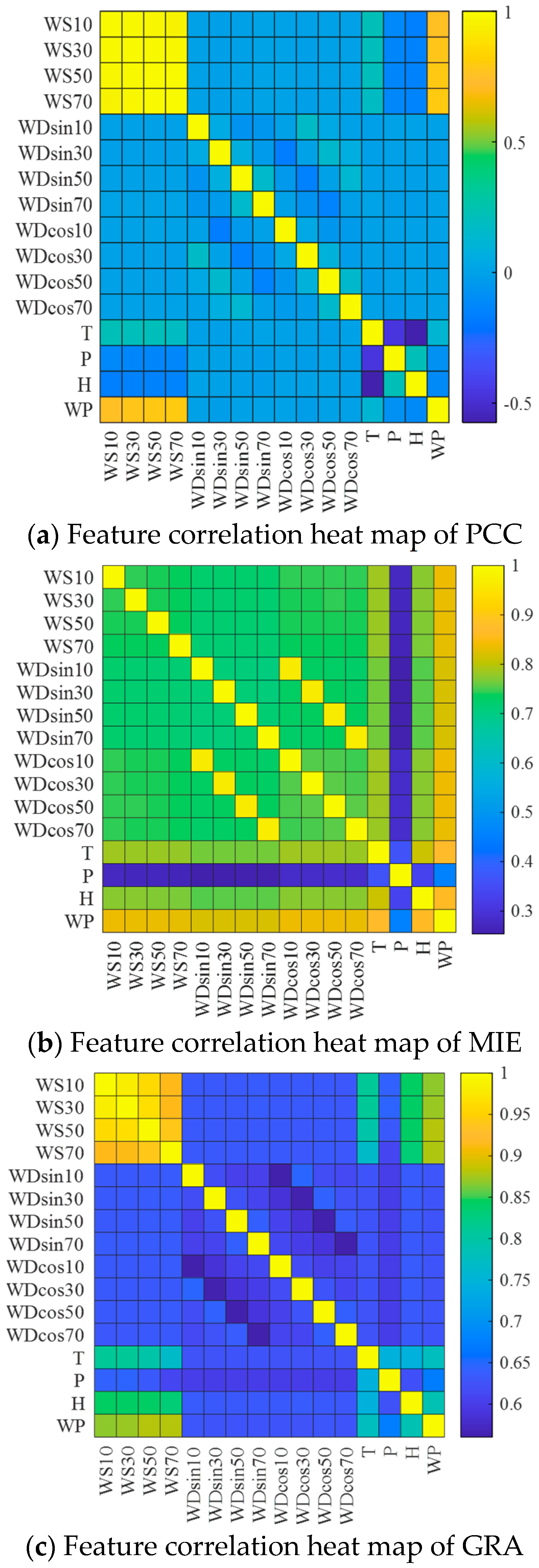
This study utilizes operational records from a 200 MW onshore wind farm in northwestern China, where turbines feature 70 m hubs, 120 m rotor spans, and 1.5 MW unit ratings. The meteorological-power dataset spans January–December 2019 with 15 min temporal resolution, generating 96 daily observations (35,040 annual entries). Each timestamp integrates 15 variables: atmospheric conditions (temperature, humidity, barometric pressure) and multi-altitude wind vectors (speed/direction at 10/30/50/70 m elevations).

Three statistical methodologies from Section 2.1 were applied to quantify both inter-variable relationships within meteorological parameters and their associations with wind energy output. Visualized in Figure 1, Figure 1a presents pairwise PCC across parameters, while Figure 1b illustrates MIE-derived nonlinear dependencies, and Figure 1c demonstrates GRA outcomes. Each matrix systematically maps meteorological parameter interactions alongside meteorological-parameters–power-linkages through distinct mathematical frameworks.

It can be seen from Figure 1 that the values of PCC, MIE, and GRA between wind speed and direction (including wind speed and direction (WS & D) at 10 m, 30 m, 50 m, and 70 m) and the wind power are all relatively large, indicating that WS & D are one of the main features affecting the wind power. From Figure 1, we also find that the correlations between WS & D at 10 m, 30 m, 50 m, and 70 m are very strong, indicating the existence of redundancy among these WS & D. Since the hub height of wind turbines is 70 m, this paper selects the WS & D at 70 m as the input features of the forecasting model. In addition, it can be seen from Figure 1a that the values of PCC between temperatures, air pressure and humidity, and wind power are small, indicating that their linear correlations with wind power are poor. It can be seen from Figure 1b that the values of MIE between air pressure and wind power are small, further proving that the correlation between air pressure and wind power is poor.

Table 1. Correlation degree between NWP data characteristics and wind power.

NWP Data Characteristics	PCC	MIE	GRA
WS 10 m	0.75	0.837	0.8692
WS 30 m	0.78	0.836	0.8720
WS 50 m	0.79	0.835	0.8805
WS 70 m	0.80	0.832	0.8802
WD 10 m sine	0.0014	0.8198	0.6292
WD 30 m sine	0.0146	0.8205	0.6282
WD 50 m sine	0.004	0.8212	0.6288
WD 70 m sine	0.0065	0.8206	0.6285
WD 10 m cosine	0.005	0.8373	0.6285
WD 30 m cosine	0.0113	0.8376	0.6270
WD 50 m cosine	0.0036	0.8377	0.6295
WD 70 m cosine	0.0035	0.8367	0.6283
Temperature	0.12	0.870	0.7758
Sea level pressure	0.078	0.454	0.6741
Humidity	0.11	0.862	0.7884

presents the correlation between NWP data features and wind power. The values of PCC, MIE, and GRA for WS & D at 70 m show strong correlations with wind power, validating their selection as key input features for the forecasting model. Additionally, based on the correlation analysis of temperature, pressure, and humidity with wind power, temperature and humidity are also included as input features in the model.

Based on the analysis in Figure 1 and Table 1, five NWP data features—WS & D at 70 m (direction represented by sine and cosine), temperature, and humidity—are selected as the input features for the forecasting model.

2.3. Data Clustering of Similar Days

Daily data with similar distribution patterns are grouped into clusters, which are then used to train and test the forecasting model. This approach preserves the temporal correlation of the data while enhancing the model’s forecasting accuracy. To achieve clustering, the Gaussian mixture model (GMM) is applied to the selected NWP and wind power features. The GMM clustering algorithm is described in Equation (5).

$$P(x_i)={\displaystyle \sum _{k=1}^K{\pi }_k\phi (x_i, {\mu }_k, {\sum }_k)}$$

(5)

In Equation (5), $P(x_i)$ represents the probability density function of the GMM, $x_i$ is the distribution characteristic of the i-th daily data, ${\pi }_k$ is the weight of the k-th Gaussian probability density function, ${\mu }_k$ and ${\sum }_k$ are the mean and covariance matrix of the k-th Gaussian probability density function, respectively, and K is the number of Gaussian models.

When using the GMM for clustering, a reasonable number of clusters is the key to improving the accuracy of WPF. When the number value of clusters is large, the number of samples in each cluster is small, resulting in an under-learning phenomenon in the forecasting model and affecting the accuracy of the forecasting model. When the number value of clusters is small, there is a situation where multiple clusters of data are merged into one cluster, causing an over-learning phenomenon in the model and affecting the accuracy of forecasting model. In order to select a reasonable number of clusters, this paper calculates the sum of the squared errors of samples under the different numbers of clusters. When the sum of the squared errors of samples and the number of clusters reach the best balance point, the obtained number of clusters is the optimal number of clusters for the samples. The calculation formula for the sum of the squared errors of samples is shown in Equation (6).

$$E_{ss}={\displaystyle \sum _{i=1}^M{\displaystyle \sum _{x\in C_i}{\left|x-m_i\right|}^2}}$$

(6)

In Equation (6), $E_{ss}$ represents the sum of the squared errors of samples, $M$ is the number of clusters, $C_i$ is the samples of the i-th cluster, and $m_i$ is the mean of the samples of the i-th cluster.

Figure 2a shows the quantitative relationship curve between the sum of the squared errors of samples $E_{ss}$ and the number of clusters $M$. As can be seen from Figure 2a, when the number of clusters $M$ is 4, the sum of the squared errors of the samples $E_{ss}$ and the number of clusters $M$ are at the best balance point. Figure 2b shows the clustering results of similar-day data. As can be seen from Figure 2b, using the clustering strategy described in this section can effectively cluster the similar-day data into four clusters. The number of similar-day samples in each clustered sample set is 78, 86, 110, and 86, respectively (after removing some abnormal data, the complete number of daily data is 360).

3. Data Empirical Wavelet Transform

3.1. Principles of Empirical Wavelet Transform

The NWP and wind power data exhibit significant randomness and volatility, which are key factors influencing forecasting accuracy. These characteristics are primarily manifested as high-frequency components in the frequency domain. To address this, empirical wavelet transform (EWT) is applied to decompose the data into different frequency components, facilitating the extraction of the high-frequency elements. The decomposed frequency data are then used for model training and testing, and the results are combined to produce the final forecast.

In the EWT, the detail coefficient $W_f^{\epsilon }\left(n,t\right)$ of the EWT is obtained by the inner product of the empirical wavelet function ${\psi }_n(\omega )$ and the original data sequence $f\left(t\right)$, as shown in Equation (7).

$$W_f^{\epsilon }\left(n,t\right)=〈f,{\psi }_n〉={\displaystyle \int f\left(\tau \right)}\overline{{\psi }_n\left(\tau -t\right)}d\tau =F^{-1}\left[f\left(\omega \right)\overline{{\psi }_n\left(\omega \right)}\right]$$

(7)

The approximation coefficient $W_f^{\epsilon }\left(0,t\right)$ of the EWT is obtained by the inner product of the empirical scale function ${\varphi }_n(\omega )$ and the original data sequence $f\left(t\right)$, as shown in Equation (8).

$$W_f^{\epsilon }\left(0,t\right)=〈f,{\phi }_1〉={\displaystyle \int f\left(\tau \right)}\overline{{\phi }_1\left(\tau -t\right)}d\tau =F^{-1}\left[f(\omega )\overline{{\phi }_1\left(\omega \right)}\right]$$

(8)

where $\overline{{\psi }_n(\omega )}$ and $\overline{{\phi }_1(\omega )}$ are the conjugate functions of ${\psi }_n(\omega )$ and ${\phi }_1(\omega )$, respectively, and $F^{-1}\left[ \right]$ represents the inverse Fourier transform.

The reconstruction expression of the NWP data and wind power data $f\left(t\right)$ is shown in Equation (9).

$$\begin{array}{ll}f(t)& =W_f^{\epsilon }\left(0,t\right)\ast {\phi }_1\left(t\right)+{\displaystyle \sum _{n=1}^N{W}_f^{\epsilon }\left(n,t\right)\ast {\psi }_n\left(t\right)}\\ & =W_f^{\epsilon }\left(0,\omega \right)\ast {\phi }_1\left(\omega \right)+{\displaystyle \sum _{n=1}^N{W}_f^{\epsilon }\left(n,\omega \right)\ast {\psi }_n\left(\omega \right)}\end{array}$$

(9)

Thus, the expressions of the subsequences $x_k\left(t\right)$ obtained by decomposing the NWP data and wind power data $f\left(t\right)$ can be obtained as shown in Equations (10) and (11).

$$x_0\left(t\right)=W_f^{\epsilon }\left(0,t\right)\ast {\phi }_1\left(t\right)$$

(10)

$$x_k\left(t\right)=W_f^{\epsilon }\left(k,t\right)\ast {\psi }_k\left(t\right)$$

(11)

3.2. Data Analysis of Empirical Wavelet Transform

Figure 3a illustrates the reconstruction error distribution after decomposing the wind power data using the EWT method. When the data are decomposed into three or more subsequences, the reconstruction errors remain consistent, indicating that the decomposition does not affect the reconstruction performance beyond three subsequences. To minimize forecasting errors and computational time, NWP and wind power data are decomposed into three subsequences. Figure 3b displays the three subsequences derived from the wind power data using the EWT technique. Among them, Subsequence A1 is the high-frequency component, Subsequence A2 is the medium-frequency component, and Subsequence A3 is the low-frequency component. As shown in Figure 3b, the high-frequency components primarily describe the stochasticity of NWP and wind power data, while the low-frequency components mainly describe the fluctuations in NWP and wind power data.

4. Evaluation Indicators of Interval Forecasting Performance

4.1. Performance Evaluation Indicators of Interval Forecast

Probabilistic WPF aims to produce uncertainty bounds that optimally balance coverage reliability (encompassing maximal observed values) and interval sharpness (minimized bandwidth). Performance quantification relies on three statistical benchmarks: prediction interval coverage probability (PICP) for reliability assessment, normalized average width (PINAW) for sharpness evaluation, and the coverage-width criterion (CWC) for hybrid optimization. This section delineates their mathematical formulations and validation framework.

(1) Prediction interval coverage probability

The PICP serves as a fundamental performance indicator in uncertainty quantification, measuring the likelihood that observed wind power outputs fall within the defined uncertainty range. Superior PICP magnitudes directly correlate with increased observational containment, signifying enhanced capability to probabilistically encapsulate operational variability. Its computational methodology is formalized in Equation (12).

$$\mathrm{PICP}={\displaystyle \frac{1}{N}}{\displaystyle \sum _{i=1}^N{k}_i}$$

(12)

Among them, N is the number of wind power prediction points; $k_i$ is the coverage factor. When the actual power falls within the prediction interval, $k_i=1$, otherwise $k_i=0$. In practical applications, the PICP value usually needs to be greater than the predefined confidence level.

(2) Prediction interval normalized average width

If we simply pursue the PICP, it may lead to excessive bandwidth of the prediction interval, thereby losing practical value. For this reason, the index of the PINAW is introduced to measure the bandwidth of the prediction interval. The calculation formula of the PINAW is shown in Equation (13).

$$\mathrm{PINAW}={\displaystyle \frac{1}{NR}}{\displaystyle \sum _{i=1}^N\left(U_i-L_i\right)}$$

(13)

In Equation (13), $U_i$ is the upper bound of the interval, $L_i$ is the lower bound of the interval, R is the variation range of the target value and is used for normalizing the average bandwidth.

(3) Coverage width criterion

PICP and PINAW are opposing metrics in interval forecasting. Increasing PICP typically leads to a rise in PINAW, while reducing PINAW results in a decrease in PICP. To provide a more balanced assessment of the prediction interval’s performance, both PICP and PINAW are combined into the CWC evaluation metric. The formula for calculating CWC is given in Equation (14).

$$\mathrm{CWC}=\left\{\begin{array}{ll}\mathrm{PINAW} & \mathrm{PICP}\ge \mu \\ \mathrm{PINAW}(1+e^{-\eta (\mathrm{PICP}-\mu )})& \mathrm{PICP}<\mu \end{array}\right.$$

(14)

In Equation (14), $\mu$ is the preset interval confidence level, and $\eta$ is the penalty parameter, which is used to penalize the situation where the PICP indicator is lower than the interval confidence level.

4.2. Construction of Loss Function

The objective of wind power interval forecasting is to maximize PICP while minimizing PINAW. To achieve this, a loss function incorporating both PICP and PINAW is proposed in this paper. The loss function is presented in Equation (15).

$$\mathrm{Loss}={\displaystyle \frac{1}{NR}}{\displaystyle \sum _{i=1}^N\left(U_i-L_i\right)}\cdot k_i+{\displaystyle \frac{\lambda N}{\alpha (1-\alpha )}}\max {(0,\left(1-\alpha \right)-\mathrm{PICP})}^2$$

(15)

In Equation (15), $\lambda$ is the penalty factor and $1-\alpha$ is the confidence level of the prediction interval. It can be seen from Equation (15) that when the PICP value is lower than the confidence level, the value of the loss function is large; when the PICP value is greater than or equal to the confidence level, in order to reduce the value of the loss function, the bandwidth of the prediction interval can be reduced. When Equation (15) is at the minimum value, the corresponding PICP and PINAW are the optimal values.

5. Construction of Interval Forecasting Model

5.1. Convolutional Neural Network

The CNN reduces the number of parameters and data dimensions while extracting spatial features from the input data through techniques like local connections, weight sharing, and pooling. These operations enhance the computational efficiency and analytical capabilities of the CNN. The network consists of an input layer, convolutional layer, pooling layer, fully connected layer, and output layer, as illustrated in Figure 4.

The input layer is mainly used to obtain the input data of the CNN. The input data in this paper are the NWP data and wind power data, which are a data matrix of N × M, where N is the time series length of the data and M is the NWP feature data and wind power data at each time point.

As a core component of CNNs, the convolutional operation specializes in capturing diverse meteorological patterns and spatial relationships linking wind energy outputs with NWP information. Our architecture incorporates dual convolutional modules—the initial layer applies 16 3 × 3 kernel filters while the subsequent layer employs 32 3 × 5 dimensional matrices to analyze the combined input sources.

The pooling layer reduces the dimensionality of the input data, enhancing CNN computation speed and mitigating overfitting. Common pooling methods include max-pooling, mean-pooling, and stochastic-pooling. Given the distribution characteristics of wind power and NWP data, this study adopts the max-pooling method.

The fully connected layer links each neuron to all neurons in the preceding layer, integrating local features from the convolutional or pooling layers into global features. The output layer then generates the spatial correlation features of the wind power and NWP data extracted by the CNN.

5.2. BiGRU Calculation Principle and Model Structure

5.2.1. Calculation Principle of GRU

The GRU model, a variant of the LSTM, shares its ability to handle time series data effectively, addressing issues like vanishing and exploding gradients. Compared to LSTM, the GRU requires fewer parameters, offers faster training, and reduces overfitting, making it particularly efficient for time series forecasting. This paper employs the GRU model for day-ahead WPF. The model’s structure is shown in Figure 5.

The GRU model is mainly composed of two parts: the update gate $z_t$ and the reset gate $r_t$. The process of data processing implemented by the GRU model is as follows:

(1) The update gate $z_t$ controls the extent to which the information from the previous moment is retained at the current moment. The larger the output value of the update gate $z_t$, the more information from the previous moment is retained. The calculation formula of the update gate $z_t$ is as expressed in Equation (16).

$$z_t=\sigma (w_z\cdot [h_{t-1}, x_t]+b_z)$$

(16)

In Equation (16), $\sigma (\cdot )$ is the sigmoid function, $w_z$ is the weight of the update gate, $h_{t-1}$ is the hidden state of the previous moment, $x_t$ is the current moment input, and $b_z$ is the bias value.

(2) The reset gate $r_t$ controls how much of the information from the previous moment is retained on the current moment candidate hidden state ${\tilde{h}}_t$. The larger the output value of the reset gate $r_t$, the more information from the previous moment is retained in the candidate hidden state ${\tilde{h}}_t$. The calculation formula of the reset gate $r_t$ is as expressed in Equation (17).

$$r_t=\sigma (w_r\cdot [h_{t-1}, x_t]+b_r)$$

(17)

In Equation (17), $w_r$ is the weight of the reset gate and $b_r$ is the bias value.

(3) The update of the candidate hidden state information ${\tilde{h}}_t$ is as expressed in Equation (18).

$${\tilde{h}}_t=\tanh (w_h\cdot [r_t\odot h_{t-1}, x_t]+b_h)$$

(18)

In Equation (18), $\tanh (\cdot )$ is the activation function, $w_h$ is the weight of the candidate hidden state, and $b_h$ is the bias value of the candidate hidden state.

(4) Calculate the current moment hidden state $h_t$ based on ${\tilde{h}}_t$ and $h_{t-1}$:

$$h_t=(1-z_t)\odot h_{t-1}+z_t\odot {\tilde{h}}_t$$

(19)

5.2.2. BiGRU Model Structure

The GRU model effectively captures the forward features of time series data. However, time series data are also influenced by past data, not just future values. To capture both forward and backward dependencies, the bidirectional gated recurrent unit (BiGRU) model is proposed. This model integrates both forward and backward GRU components to better analyze the relationships in time series data.

Figure 6 illustrates the structure of the BiGRU model, which consists of an input layer, a forward GRU, a backward GRU, and an output layer. The forward and backward GRUs capture information from the respective forward and backward sequences of the input data. The calculation process of the BiGRU model is detailed in Equations (20)–(22).

$${\overrightarrow{h}}_t=f(x_t, {\overrightarrow{h}}_{t-1})$$

(20)

$${\overleftarrow{h}}_t=f(x_t, {\overleftarrow{h}}_{t-1})$$

(21)

$$Q_t=\overrightarrow{w}{\overrightarrow{h}}_t+\overleftarrow{w}{\overleftarrow{h}}_t+b_t$$

(22)

In Equation (22), $\overrightarrow{w}$ and $\overleftarrow{w}$ are the weights of the output of the forward GRU hidden layer and the output of the backward GRU hidden layer, respectively, and $b_t$ is the bias value of the BiGRU model.

5.3. Multi-Head Self-Attention Mechanism

The multi-head self-attention mechanism (MHSAM) generates multiple data sequences by applying different linear projections to the original data. Each projection, or “head”, captures distinct features of the data. These sequences are then concatenated and passed through another linear projection to form the final sequence.

For the input data sequence $X=[x_1, x_2, x_3, \cdots , x_m]$, multiply the input data sequence by the linear transformation matrices $W_j^Q$, $W_j^K$, and $W_j^V$, respectively to obtain the vectors $Q_j$, $K_j$, and $V_j$, $j\in (1, 2, 3, \cdots , N)$, and $N$ represents the number of heads of the MHSAM. The specific calculation process is shown in Equations (23)–(25).

$$Q_j=W_j^Q\cdot X$$

(23)

$$K_j=W_j^K\cdot X$$

(24)

$$V_j=W_j^V\cdot X$$

(25)

Then, the attention calculation formula of the j-th head is shown in Equation (26).

$${\mathrm{head}}_i=\mathrm{Attention}(Q_i, K_i, V_i)=\mathrm{soft}\max ({\displaystyle \frac{Q_i\cdot K_i^T}{\sqrt{N}}})\cdot V_i$$

(26)

The output of the MHSAM can be calculated by Equation (27).

$$Y{=\mathrm{Concat}(\mathrm{head}}_1{, \mathrm{head}}_2{, \mathrm{head}}_3, \cdots {, \mathrm{head}}_N)\cdot W^{\mathrm{o}}$$

(27)

In Equation (27), $W^{\mathrm{o}}$ is the output weight matrix of the MHSAM.

The model structure of the MHSAM is shown in Figure 7.

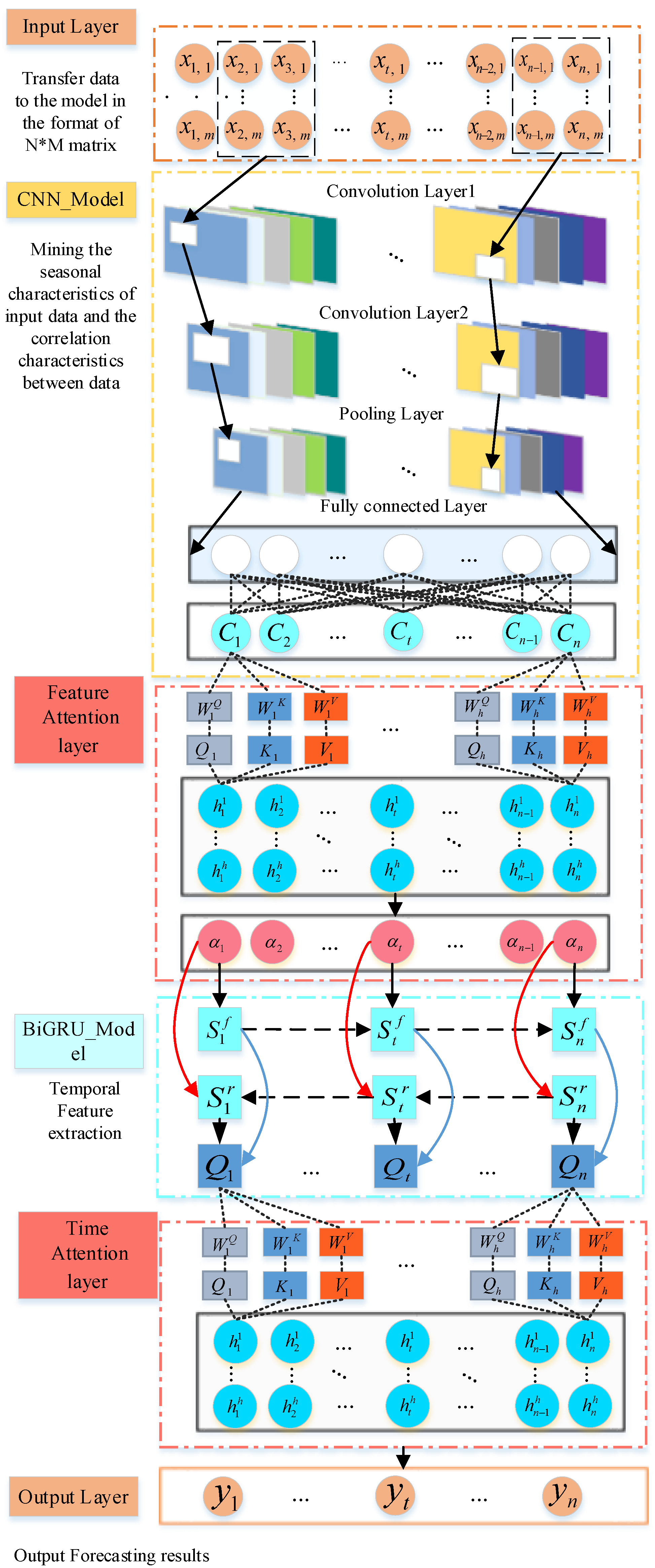
5.4. Construction of the CNN-BiGRU-MHSAM Model

This study employs the CNN model to analyze the spatial correlations between wind power and NWP data, followed by the BiGRU model to examine the temporal dependencies within the input sequence, enabling precise characterization of the temporal distribution. Subsequently, the MHSAM assigns greater weight to the critical features that influence forecasting accuracy. The CNN-BiGRU-MHSAM model integrates these components to provide an accurate day-ahead WPF. Figure 8 illustrates the structure of this model, with the functions of each component outlined below.

(1) Input layer

The input layer transmits the data in the training dataset to the model. The format of the input data is a $N\times M$ matrix, where N is the length of the time sequence of the training data and M is the data features at each time point in the time sequence.

(2) CNN model

The CNN model examines the spatial distribution of the input data using the convolutional, pooling, and fully connected layers.

(3) Feature attention mechanism layer

During model training, the attention weights of features are adaptively adjusted to analyze their contributions to wind power. Features with greater influence are emphasized, while those less relevant to wind power are minimized or excluded.

(4) BiGRU model

The BiGRU model captures the temporal dependencies in the input data sequence. The forward GRU layer examines temporal correlations in the forward direction, while the backward GRU layer analyzes them in reverse order.

(5) Temporal attention mechanism layer

The temporal attention mechanism dynamically assigns attention weights to each time point in the time series, emphasizing the features most influential to wind power.

(6) Output layer

The output layer outputs the model’s forecasting results.

6. Construction of the Interval Forecasting Model

The construction of the interval forecasting model proceeds as follows:

Step 1: Data preprocessing

Remove any anomalies in the NWP and wind power data to minimize their impact on forecasting accuracy.

Step 2: Feature selection of NWP data

Based on the strategy outlined in Section 2, select five key features from the NWP data, including wind speed at 70 m, wind direction (represented by sine and cosine), temperature, and humidity, as input for the forecasting model.

Step 3: Similar-day data clustering

According to the data-clustering strategy in Section 2, GMM is used to cluster the NWP data and wind power data into four clusters.

Step 4: Division of training dataset and testing dataset

The NWP data and wind power data in each cluster are divided into training dataset and testing dataset. In the first cluster dataset, the data of February 2nd are selected as the testing dataset. In the second cluster dataset, the data of 13 June are selected as the testing dataset. In the third cluster dataset, the data of 29 May are selected as the testing dataset. In the fourth cluster dataset, the data of 31 August are selected as the testing dataset. The remaining data are all used as the training datasets.

Step 5: Calculate the upper and lower bounds of the WPF interval

According to the statistical distribution characteristics of wind power in each cluster dataset, calculate the upper bound value $u_{\alpha }$ and lower bound value $l_{\alpha }$ of the confidence interval of wind power at different confidence levels in each cluster dataset. According to Equation (28), the upper bound value $U_i^{\alpha }$ and lower bound value $L_i^{\alpha }$ of the wind power data point of each cluster can be obtained.

$$\left\{\begin{array}{l}{U}_i^{\alpha }=y_i+(u_{\alpha }-\overline{y})\\ L_i^{\alpha }=y_i-(\overline{y}-l_{\alpha })\end{array}\right.$$

(28)

In Equation (28), $y_i$ is the true value of wind power in each cluster, $\overline{y}$ is the average value of wind power in each cluster, $l_{\alpha }$ is the lower bound of the confidence interval of wind power in each cluster, and $u_{\alpha }$ is the upper bound of the confidence interval of wind power in each cluster.

Step 6: Initialize model hyperparameters

According to the value range of the model hyperparameters, randomly initialize the model hyperparameters.

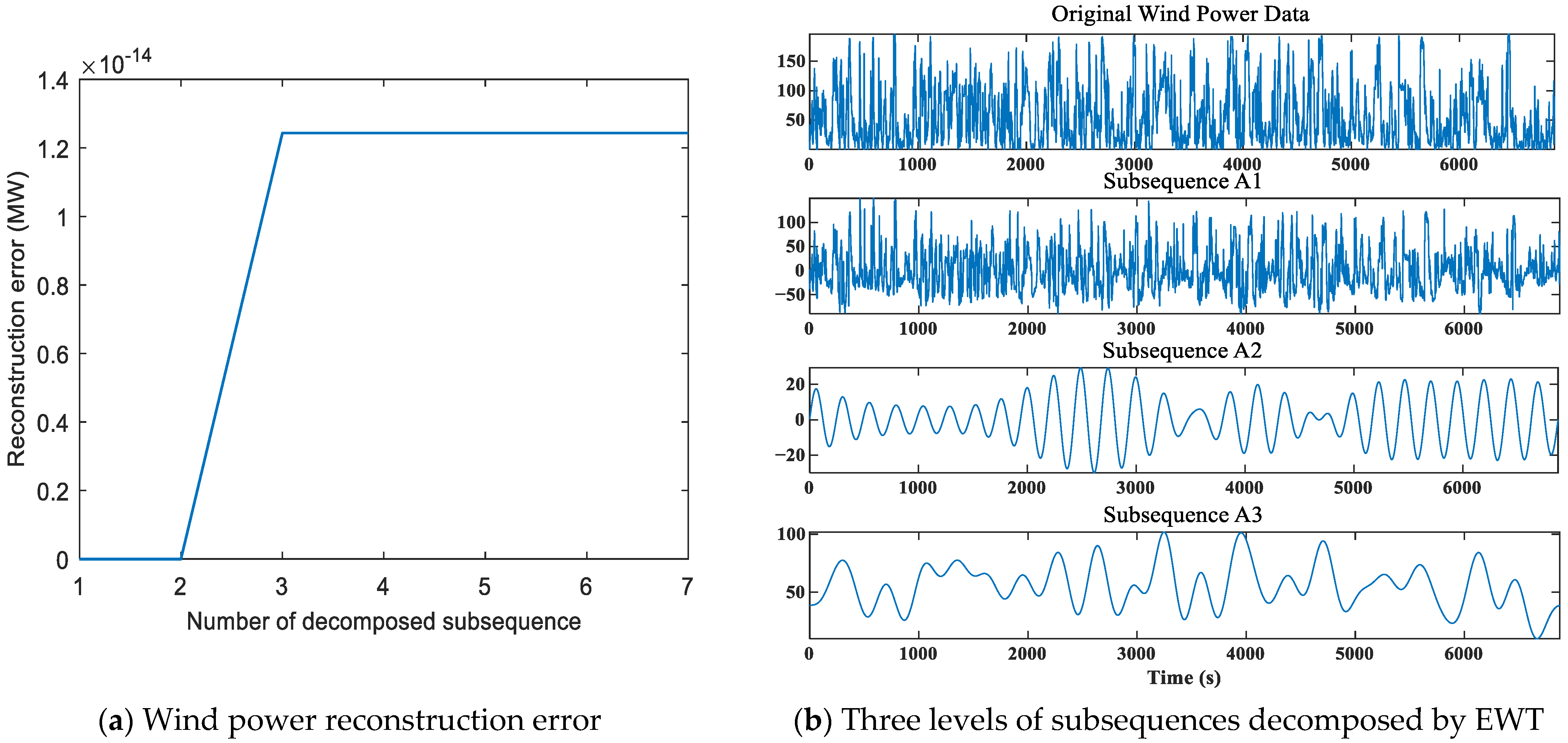
Step 7: EWT decomposition of data

According to the principle of EWT introduced in Section 3, the NWP data and the upper and lower bound data of wind power in the training dataset and the testing dataset are decomposed by EWT to obtain subsequences of different frequencies.

Step 8: Forecasting model training

Input the subsequence data after EWT decomposition of the training dataset into the CNN-BiGRU-MHSAM forecasting model to train the forecasting model.

Step 9: Reconstruct the upper and lower bounds of the forecast interval

According to the forecasting results of each subsequence of wind power data, reconstruct the upper and lower bounds of the day-ahead wind power interval forecast.

Step 10: Calculate the loss function of the interval forecast of training dataset

According to the loss function calculation Formula (15), calculate the loss function of the interval forecasting result of the training dataset, and save the model parameters when the loss function is the smallest.

Step 11: Adjustment of forecasting model hyperparameters

According to the convergence condition of the forecasting model, judge whether the training process meets the convergence condition. If the convergence condition is not met, then use the grid method to adjust the model hyperparameters, and then jump to Step 8 to continue execution; if the convergence condition is met, then execute Step 12.

Step 12: Testing of the forecasting Model

Use the testing dataset after EWT decomposition to test the trained model and calculate the evaluation indicators of the interval forecasting results of the testing dataset.

The construction of the entire interval forecasting model is shown in Figure 9.

7. Case Analysis

7.1. Hyperparameter Settings of the Interval Forecasting Model

In deep learning models, hyperparameters play a crucial role in determining forecasting accuracy. To select appropriate hyperparameters, this study employs the grid search method. The hyperparameter settings for each model are summarized in

Table 2. Hyperparameter setting for deep learning models.

Model	Hyper-Parameter	Range	Determined Value
CNN	Number of convolutional layers	(1, 2, 3, 4)	2
	Filters in 1st convolutional layer	(8, 16, 32)	16
	Convolutional kernel size	(3, 5, 7)	3
	Convolutional stride	(1, 2, 3)	1
	Filters in 2nd convolutional layer	(8, 16, 32)	32
	Convolutional kernel size	(3, 5, 7)	3
	Convolutional stride	(1, 2, 3)	1
	Pooling kernel size	(2, 4, 6)	2
	Units in fully connected layer	(32, 64, 128)	64
	Activation function	(Sigmoid, Tanh, ReLU)	ReLU
Feature attention mechanism	Number of MHSA layer input size	(64, 128, 256)	128
	Number of MHSA layer heads	(3, 4, 5, 6, 7, 8)	7
BiGRU	Number of BiGRU hidden layer units	(16, 32, 64, 128)	128
Time attention mechanism	Number of MHSA layer input size	(64, 128, 256)	256
	Number of MHSA layer heads	(3, 4, 5, 6, 7, 8)	5
Training Options	Solver for training network	(sgdm, rmsprop, adam)	rmsprop
	Epochs	(50, 100, 150, 200, 250)	200
	Initial learning rate	[10−5, 10−2]	0.002
	MiniBatchSize	(32, 64, 128, 256)	128

. The “Range” column indicates the search range for each hyperparameter, while the “Determined value” column presents the final chosen value.

7.2. Point Forecasting Results and Error Analysis

To demonstrate the effectiveness of the GMM-FS-EWT-CNN-BiGRU-MHSAM forecasting model, this section compares its performance with that of the GMM-EWT-CNN-BiGRU-MHSAM, GMM-FS-CNN-BiGRU-MHSAM, GMM-CNN-BiGRU-MHSAM, and CNN-BiGRU-MHSAM models. The computational resources are as follows: the computer processor has a clock speed of 1.8 GHz, with 2 GB of RAM, and the software used for computation is MATLAB 2021. Since GMM, FS, and EWT all belong to machine learning methods, the computation time for these machine learning methods can complete relevant tasks within a few seconds. Therefore, the training and forecasting time of the GMM-FS-EWT-CNN-BiGRU-MHSAM model is primarily determined by the training and forecasting time of the CNN-BiGRU-MHSAM component. It can be inferred that the training and forecasting times for these five forecasting models are almost identical.

Figure 10 presents the short-term WPF results for various models when the sample set is divided into four clusters. The red solid line represents the actual output power and the red dashed line corresponds to the forecasting results of GMM-FS-EWT-CNN-BiGRU-MHSAM, while the black, blue solid lines correspond to the forecasts from the GMM-EWT-CNN-BiGRU-MHSAM, and GMM-FS-CNN-BiGRU-MHSAM models, respectively. The black dashed line shows the forecast from the GMM-CNN-BiGRU-MHSAM model, and the blue dashed line represents the forecast from the CNN-BiGRU-MHSAM model. As shown in Figure 10, all five models accurately predict the day-ahead wind power trends across different clustering scenarios, demonstrating the effectiveness of deep learning in WPF. Additionally, the proposed GMM-FS-EWT-CNN-BiGRU-MHSAM model outperforms the other models in capturing the wind power variation more precisely.

Table 3. Model forecasting error values under different clusters.

Cluster ID	Model	PMAE	PRMSE
First	GMM-FS-EWT-CNN-BiGRU-MHSAM	3.06%	3.93%
	GMM-EWT-CNN-BiGRU-MHSAM	3.40%	4.36%
	GMM-FS-CNN-BiGRU-MHSAM	3.48%	4.56%
	GMM-CNN-BiGRU-MHSAM	4.79%	6.47%
	CNN-BiGRU-MHSAM	5.43%	7.76%
Second	GMM-FS-EWT-CNN-BiGRU-MHSAM	1.17%	1.54%
	GMM-EWT-CNN-BiGRU-MHSAM	1.22%	1.63%
	GMM-FS-CNN-BiGRU-MHSAM	1.30%	1.94%
	GMM-CNN-BiGRU-MHSAM	1.32%	1.78%
	CNN-BiGRU-MHSAM	1.61%	2.44%
Third	GMM-FS-EWT-CNN-BiGRU-MHSAM	1.83%	2.67%
	GMM-EWT-CNN-BiGRU-MHSAM	2.00%	2.99%
	GMM-FS-CNN-BiGRU-MHSAM	2.11%	3.92%
	GMM-CNN-BiGRU-MHSAM	2.40%	3.20%
	CNN-BiGRU-MHSAM	3.26%	5.45%
Fourth	GMM-FS-EWT-CNN-BiGRU-MHSAM	2.64%	3.54%
	GMM-EWT-CNN-BiGRU-MHSAM	2.81%	3.74%
	GMM-FS-CNN-BiGRU-MHSAM	2.89%	3.68%
	GMM-CNN-BiGRU-MHSAM	3.24%	4.19%
	CNN-BiGRU-MHSAM	4.53%	5.92%
Error average	GMM-FS-EWT-CNN-BiGRU-MHSAM	2.18%	2.92%
	GMM-EWT-CNN-BiGRU-MHSAM	2.36%	3.18%
	GMM-FS-CNN-BiGRU-MHSAM	2.45%	3.53%
	GMM-CNN-BiGRU-MHSAM	2.94%	3.91%
	CNN-BiGRU-MHSAM	3.71%	5.39%

presents the day-ahead WPF error values for various clustering samples. As shown in Table 3, the GMM-FS-EWT-CNN-BiGRU-MHSAM model exhibits the smallest forecasting error, indicating its superior accuracy compared to the other models. This further confirms the effectiveness and advantages of the proposed GMM-FS-EWT-CNN-BiGRU-MHSAM forecasting model.

As shown in Table 3, the forecasting accuracy of the GMM-CNN-BiGRU-MHSAM model is higher than that of the CNN-BiGRU-MHSAM model. It can be inferred that clustering daily data with similar distribution characteristics using the GMM model can effectively improve the accuracy of WPF. The forecasting accuracy of the GMM-FS-CNN-BiGRU-MHSAM model is higher than that of the GMM-CNN-BiGRU-MHSAM model, indicating that selecting appropriate meteorological features for WPF is also an effective way to enhance forecasting accuracy. The forecasting accuracy of the GMM-EWT-CNN-BiGRU-MHSAM model is higher than that of the GMM-CNN-BiGRU-MHSAM model, proving that using EWT to decompose numerical weather prediction data and wind power data into frequency data containing temporal information, and extracting high-frequency components that represent randomness and volatility in the data, is also an important strategy for improving WPF.

Based on the case study analysis above, it can be seen that the forecasting model proposed in the paper has good forecasting performance in time series data forecast. However, we must point out that when these time series data are significantly missing, the forecasting accuracy of the proposed model will be affected, and its forecasting accuracy may even be lower than that of conventional machine learning models. Additionally, since this paper uses the EWT to remove high-frequency components from numerical weather prediction data and wind power data, the prediction accuracy of the model is bound to decrease in the event of extreme weather conditions.

7.3. Analysis of Interval Forecasting Results

To demonstrate the accuracy and superiority of the GMM-FS-EWT-CNN-BiGRU-MHSAM model, a comparative analysis with the non-parametric kernel density estimation method is conducted. The interval forecasting results for day-ahead wind power across four clustering samples at confidence levels of 97.5%, 95%, 90%, and 80% are presented in

Table 4. Interval forecasting results for the first cluster at different confidence levels.

Methods	Indicators	Confidence Level
		97.5%	95%	90%	80%
Proposed Model	PICP	100%	100%	100%	90.63%
	PINAW	0.2269	0.1895	0.1482	0.098
	CWC	0.2269	0.1895	0.1482	0.098
NPKDE	PICP	100%	98.96%	94.79%	73.96%
	PINAW	0.6854	0.5667	0.4261	0.2505
	CWC	0.6854	0.5667	0.4261	0.4936

,

Table 5. Interval forecasting results for the second cluster at different confidence levels.

Methods	Indicators	Confidence Level
		97.5%	95%	90%	80%
Proposed Model	PICP	100%	100%	96.88%	89.58%
	PINAW	0.4515	0.3783	0.2448	0.1478
	CWC	0.4515	0.3783	0.2448	0.1478
NPKDE	PICP	100%	95.83%	15.63%	0%
	PINAW	4.7935	4.4328	3.8805	2.7360
	CWC	4.7935	4.4328	6.5559	4.5700

,

Table 6. Interval forecasting results for the third cluster at different confidence levels.

Methods	Indicators	Confidence Level
		97.5%	95%	90%	80%
Proposed Model	PICP	100%	98.96%	98.96%	88.54%
	PINAW	0.2048	0.1663	0.1149	0.065
	CWC	0.2048	0.1663	0.1149	0.065
NPKDE	PICP	100%	97.92%	61.46%	0%
	PINAW	0.7894	0.6804	0.5494	0.3183
	CWC	0.7894	0.6804	1.0257	0.5316

and

Table 7. Interval forecasting results for the fourth cluster at different confidence levels.

Methods	Indicators	Confidence Level
		97.5%	95%	90%	80%
Proposed Model	PICP	100%	100%	100%	93.67%
	PINAW	0.2566	0.2219	0.1817	0.1334
	CWC	0.2566	0.2219	0.1817	0.1334
NPKDE	PICP	93.67%	87.34%	75.95%	55.70%
	PINAW	0.5148	0.4061	0.2643	0.1393
	CWC	1.02	0.7969	0.5107	0.2626

. As shown in these tables, the GMM-FS-EWT-CNN-BiGRU-MHSAM model successfully reduces interval width while maintaining a high coverage rate, confirming its effectiveness and superiority in interval forecasting.

Figure 11 illustrates the distribution of forecasting intervals for the GMM-FS-EWT-CNN-BiGRU-MHSAM model at confidence levels of 97.5%, 95%, 90%, and 80% across different weather clusters. As shown, although a small portion of the actual wind power values fall outside the forecasted interval—likely due to factors such as NWP errors or sudden weather changes that cause significant deviations between forecasted and actual power—the majority of the values remain within the intervals, with a probability exceeding the confidence level. This confirms that the proposed interval forecasting model accurately captures the variation range of actual wind power.

8. Conclusions

In this paper, a day-ahead wind power interval forecasting model based on GMM-FS-EWT-CNN-BiGRU-MHSAM is proposed. This model uses the FS to select the key features that affect the forecasting accuracy of wind power, and uses the GMM to cluster the data with similar meteorological features into one cluster. On this basis, the EWT is used to decompose the NWP data and wind power data into frequency data with time information to extract the high-frequency components in the data. The GMM-FS-EWT-CNN-BiGRU-MHSAM forecasting model is constructed by integrating the CNN, BiGRU, and MHSAM. The calculation results show the following:

(1) Performing feature selection on NWP data and then clustering NWP data and wind power data using the GMM model can effectively improve the forecasting accuracy of day-ahead wind power.

(2) The use of empirical wavelet transform to decompose NWP and wind power data into frequency components with time information allows for the extraction of high-frequency data, which enhances the forecasting accuracy.

(3) A CNN is used to extract spatial correlations and meteorological features, while the BiGRU model captures temporal dependencies within the data sequence. A MHSAM is incorporated to assign greater weight to the most influential elements.

(4) The GMM-FS-EWT-CNN-BiGRU-MHSAM model reduces interval width while maintaining the coverage rate of the forecasting intervals, and the examples demonstrate that the method proposed in this paper has good forecasting performance.