Research on Online Energy Management Strategy for Hybrid Energy Storage Electric Vehicles Under Adaptive Cruising Conditions

Abstract

To address the critical challenge of high energy consumption in single-source electric vehicles, this study proposes a hybrid energy storage system (HESS)-integrated energy management strategy (EMS). Firstly, the car-following and HESS models are constructed. Secondly, a multi-objective optimization framework balancing adaptive cruise control (ACC) optimal tracking quality and energy economy is developed, where the fast, non-dominated sorting genetic algorithm (NSGA-II) resolves dynamic power demands. Thirdly, the third-order Haar wavelet enables online rolling decomposition of power profiles. The high-frequency transient power is matched by a supercapacitor, while the low-frequency steady-state power is utilized as an input variable to the optimization controller. Then, a fuzzy logic controller dynamically optimizes HESS’s energy distribution based on state-of-charge (SOC) and load conditions. Finally, the cruise simulation model has been constructed utilizing the MATLAB/Simulink platform. Comparative analysis under the Urban Dynamometer Driving Schedule (UDDS) demonstrates a 3.71% reduction in the total power demand of the ego vehicle compared to the front vehicle. Compared to single-source configurations, the HESS ensures smoother SOC dynamics in lithium-ion batteries. After employing the third-order Haar wavelet for online rolling decomposition of the demand power, the high-frequency transient power matched by the lithium-ion battery is substantially reduced. Comparative analysis of three control strategies demonstrates that the wavelet-fuzzy logic approach exhibits superior comprehensive performance. Consequently, the proposed strategy effectively mitigates high-frequency transient peak charge/discharge currents in the lithium-ion battery and the energy consumption of the entire vehicle. This study provides a novel solution for energy storage systems in hybrid energy storage electric vehicles (HESEV) under ACC scenarios.

1. Introduction

In recent years, with the rapid development of new energy and intelligent vehicles, the energy consumption of vehicles under adaptive cruise control (ACC) conditions has long been a focus of attention. Most researchers have adopted a dual-layer controller framework integrating ACC and energy management strategy (EMS) to hierarchically optimize vehicle energy consumption. This strategy effectively minimizes energy expenditure while driving operations and maintaining dynamic performance. Peng et al. [1] developed an ecological driving strategy (DDPG-ECO) using a deep deterministic policy gradient framework. Experimental results demonstrated that the DDPG-ECO algorithm enhanced fuel economy relative to conventional ACC systems while maintaining car-following safety. Chen et al. [2] employed distributed model predictive control (DMPC) for cooperative speed planning in the upper layer and a rolling optimization method for hybrid energy storage systems (HESS) and EMS in the lower layer. Verification demonstrated that the proposed method achieved stable vehicle cooperative control, reduced battery discharge power fluctuations, and extended battery lifespan. Zhu et al. [3] designed an ACC controller using backstepping techniques for connected and automated fuel cell/battery hybrid electric vehicles (FCHEVs) to accurately track optimal following distances. Simultaneously, they implemented an EMS based on an equivalent consumption minimization strategy (ECMS) to coordinate output power between fuel cells and lithium-ion batteries, enhancing fuel economy. Kural et al. [4] proposed a nonlinear adaptive control strategy for parallel hybrid electric vehicles with collaborative optimization objectives encompassing energy efficiency, tracking safety, and traffic flow. This strategy adjusted power distribution between batteries and engines according to different driving scenarios, achieving improved fuel economy and driving safety. He et al. [5] developed a multi-objective collaborative optimization method based on a Pareto framework for optimizing cooperative adaptive cruise control (CACC) and EMS in hybrid electric vehicles. This method balanced conflicts among traffic flow, driving safety, energy efficiency, and driving comfort. Chu [6] introduced a hybrid cooperative control strategy for fuel cell electric vehicle (FCEV) platoons. This approach employs nonlinear adaptive methods to predict vehicle speed and acceleration while integrating predictive information into the equivalent consumption minimization strategy (ECMS) to enhance real-time energy management.

Beyond the hierarchical ACC/EMS control framework, scholars have proposed various solutions for minimal energy consumption. Aljohani et al. [7] developed a real-time metadata-based optimization method for EMS in fuel cell electric vehicle platoons, integrating vehicle dynamics modeling with optimal control strategies. By predicting vehicle speed and acceleration, this method proactively adjusted battery charging/discharging states to fully utilize battery energy. Özge et al. [8] implemented a Q-learning algorithm based on reinforcement learning to reduce energy consumption in cruising conditions through vehicle route planning. Lu [9] proposed an efficient ACC model (E3DM) for car-following control in mixed traffic flows. By adjusting the following distances, E3DM maintained efficient regenerative braking. Görges et al. [10] designed an adaptive dynamic heuristic programming (ADHDP)-based ecological ACC (ECO-ACC) strategy for hybrid electric vehicles (HEVs), optimizing fuel economy and vehicle dynamic performance. In single-lane car-following scenarios, this method rapidly stabilized vehicle platoons while significantly improving fuel economy. Zhang et al. [11] proposed a dual-layer ACC architecture with hierarchical coordination. The upper layer integrates nonlinear model predictive control (NMPC) to holistically optimize cruise safety and EMS metrics, whereas the lower layer deploys hysteresis current control for precise tracking of reference signals generated by the NMPC framework. This strategy effectively reduced energy consumption and collision risks. Yu et al. [12] addressed ecological ACC (EACC) for electric vehicles by proposing a robust model predictive control (RMPC) method to handle disturbances caused by inaccurate front vehicle information. Results indicated superior economic performance compared to state-of-the-art time-domain robust MPC schemes. The aforementioned EMS primarily focuses on vehicle energy consumption under ACC conditions and has achieved favorable outcomes. However, limited research exists on high-frequency transient peak power caused by frequent acceleration/deceleration in pure electric vehicles.

The HESS adopts a dual-energy source configuration combining power batteries and supercapacitors. Capitalizing on their distinct characteristics, supercapacitors handle high-frequency transient peak power demands, while power batteries supply low-frequency steady-state power. This configuration substantially reduces the frequency of transient peak currents absorbed/released by power batteries, effectively mitigating transient current impacts on battery performance and enhancing overall energy utilization efficiency. However, the integration of dual energy sources increases the complexity of EMS. Among existing approaches, wavelet transform (WT) theory exhibits unique advantages in processing high-frequency transient power. By designing decomposition and reconstruction filters, WT separates demand power into high-frequency transient and low-frequency steady-state components, enabling precise power allocation between heterogeneous energy sources. Wang et al. [13] investigated plug-in hybrid electric vehicles with supercapacitor/lithium-ion battery HESS, studying Haar wavelet decomposition levels through simulations and validating via hardware-in-loop testing. Results demonstrated optimal performance with third-order Haar wavelet decomposition. Ibrahim et al. [14] integrated nonlinear regression neural networks with WT to advance predictive energy management. The neural networks forecasted future vehicle speeds, whereas the WT decomposed power demand profiles, thereby validating the hybrid framework’s efficacy in real-world vehicular systems. Yan et al. [15] integrated WT with logic rule control strategies in supercapacitor/battery pack configurations, achieving an 8.25% energy consumption difference compared to dynamic programming. Our research team investigated HESS’ impacts on engineering vehicles under complex working conditions, revealing that the wavelet-fuzzy logic control strategy effectively reduced energy consumption and minimized high-frequency peak current damage to batteries [16,17]. WT requires a predefined signal sequence for decomposition and reconstruction. Existing studies typically obtain demand power sequences through two methods: applying predefined operating conditions or utilizing predictions from energy management systems. However, these methods either hinder the real-time online application of WT or impose excessive computational burdens on the energy management system, thereby compromising system responsiveness.

Therefore, this study proposes an ACC-WT (Adaptive Cruise Control-Wavelet Transform) hierarchical control framework for hybrid energy storage electric vehicles (HESEV), as illustrated in Figure 1. By integrating ACC-based optimal speed planning, the framework predicts future demand power profiles, which are transmitted to the energy management system. Within the energy management system, the WT performs online rolling decomposition of the demanded power into high-frequency transient peak components and low-frequency steady-state components. The supercapacitor is dynamically allocated to handle high-frequency transient peak power demands, whereby the low-frequency steady-state power component serves as the input variable to the optimization controller. The proposed framework addresses critical challenges in battery electric vehicles during car-following operations, including frequent current fluctuations and excessive energy consumption. This establishes a foundational architecture for sustainable EMS in hybrid energy storage electric vehicles under ACC scenarios. The paper is structured into five sections: development of car-following and hybrid energy storage models (Section 1), design of the ACC control algorithm (Section 2), design of EMS for hybrid energy storage system (Section 3), validation of the ACC-WT framework performance (Section 4), and conclusions with implications for sustainable mobility (Section 5).

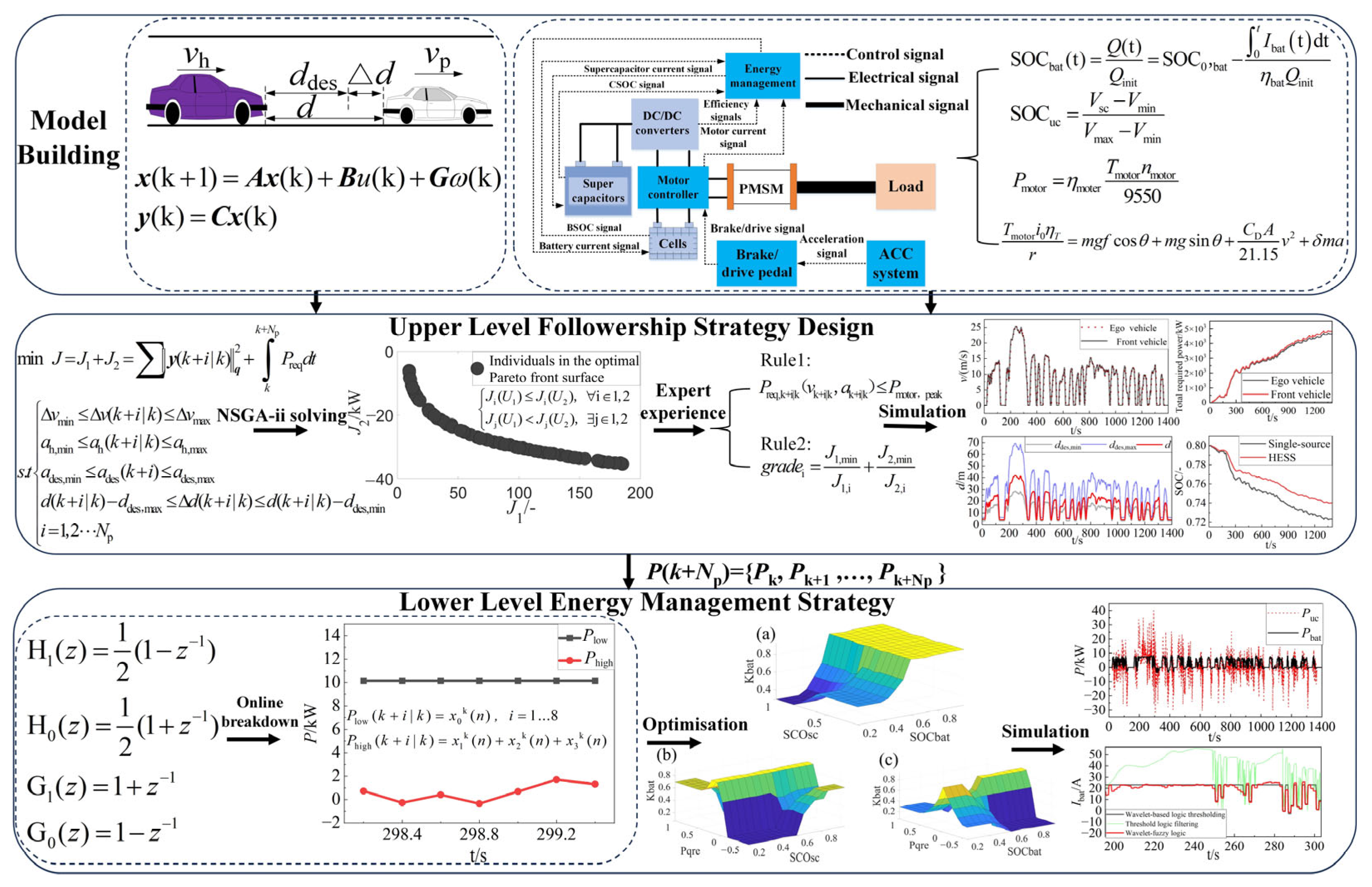
2. System Model

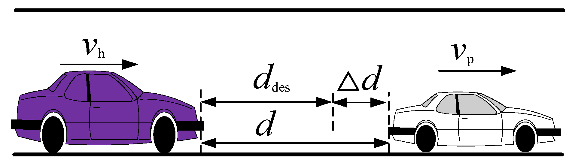
2.1. Car-Following Model

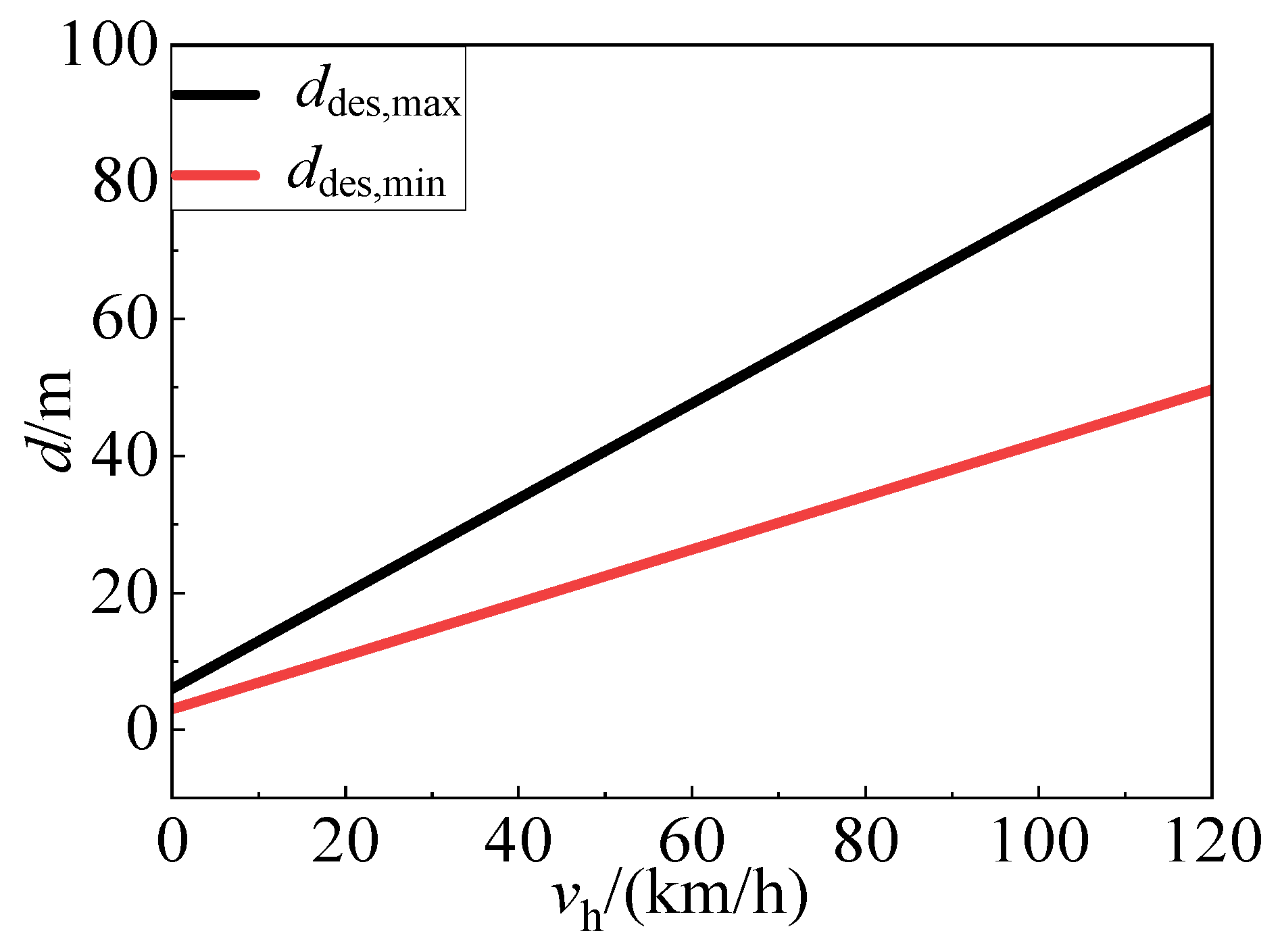
2.1.1. Expected Distance Model

In this paper, the Constant Time Headway (CTH) model [18] is selected as follows:

$$d_{\mathrm{d}\mathrm{e}\mathrm{s}}=th\times v_{\mathrm{h}}+d_0,$$

(1)

In the formula, d_des represents the desired distance; v_h denotes the ego vehicle speed; th signifies the headway time distance, which can take values from 1 to 2.5 s [18,19]; d₀ stands for the minimum gap allowed when the front vehicle and the ego vehicle completely stop, which can take values from 3 to 6 m [20]. As demonstrated in Figure 2, the upper and lower limits of the desired distance are contingent on the vehicle’s speed.

2.1.2. Car-Following Model Based on Longitudinal Kinematics

As illustrated in Figure 3, the schematic diagram of the vehicle’s adaptive cruise is presented. Utilizing kinematic principles, the distance error and relative speed expression can be derived as follows:

$$\begin{array}{l}\Delta d=d-d_{\mathrm{d}\mathrm{e}\mathrm{s}}=d-th\times v_{\mathrm{h}}-d_0\\ \Delta v=v_{\mathrm{p}}-v_{\mathrm{h}}\end{array},$$

(2)

In the formula, d stands for the actual vehicle spacing; Δd denotes the vehicle distance error; Δv represents the relative vehicle speed; v_p denotes the front vehicle speed; v_h stands for ego vehicle speed. As stated in [19], the present study examined the relationship between driver style and th vehicle following conditions. The value of 1.5 s was determined as a suitable metric for simulating a moderate driving style. Furthermore, the value of d₀ is assumed to be 4.5 m.

The derivation of Equation (2) results in the following equation:

$$\begin{array}{l}\Delta \dot{d}=\Delta v-th\times a_{\mathrm{h}}\\ \Delta \dot{v}=a_{\mathrm{p}}-a_{\mathrm{h}}\end{array},$$

(3)

In the formula, a_p represents the front vehicle acceleration; a_h stands for ego vehicle acceleration.

Furthermore, according to the first-order inertial hysteresis nature of vehicle acceleration, the desired acceleration is related to the actual acceleration by the following equation [21]:

$${\dot{a}}_{\mathrm{h}}=(K_{\mathrm{s}}{a}_{\mathrm{d}\mathrm{e}\mathrm{s}}-a_{\mathrm{h}})/T_0,$$

(4)

where K_s is the system gain, representing the steady-state tracking capability of actual acceleration to desired acceleration. To ensure consistency between actual and desired accelerations, K_s is typically set to 1 [22]. T₀ denotes the time constant, reflecting the dynamic lag from the acceleration command to the output response. Based on experimental calibration from vehicular acceleration tests, T₀ ranges between 0.3–0.6 s, with 0.45 s adopted as the nominal value to balance real-time responsiveness and energy efficiency in sustainable mobility systems [23]. a_des signifies the desired acceleration.

The state variable x is defined as [∆d, ∆v, a_h]^T, the control quantity u is given by a_des, the output quantity y is expressed as [∆d, ∆v]^T, and the disturbance quantity w is represented as a_p of the car-following system. The continuous state-space equation of the car-following system is expressed as follows:

$$\begin{array}{l}\dot{\mathit{x}}={\mathit{A}}_0\mathit{x}+{\mathit{B}}_{0}u+{\mathit{G}}_0\omega \\ \mathit{y}={\mathit{C}}_0\mathit{x}\end{array},$$

(5)

In the formula, A₀, I, B₀, G₀, and C₀ are as follows:

$${\mathit{A}}_0=\left(\begin{array}{ccc}0& 1& -th\\ 0& 0& -1\\ 0& 0& -1/T_0\end{array}\right), {\mathit{B}}_0=\left(\begin{array}{l}0\\ 0\\ K_s/T_0\end{array}\right), {\mathit{G}}_0=\left(\begin{array}{l}0\\ 1\\ 0\end{array}\right), {\mathit{C}}_0=\left(\begin{array}{ccc}1& 0& 0\\ 0& 1& 0\\ 0& 0& 1\end{array}\right)$$

Through discretization of Equation (5), the discrete state-space equation of the car-following system is derived as follows:

$$\begin{array}{l}\mathit{x}(k+1)=\mathit{A}\mathit{x}(k)+\mathit{B}u(k)+\mathit{G}\omega (k)\\ \mathit{y}(k)=\mathit{C}\mathit{x}(k)\end{array},$$

(6)

In the formula, A denotes the matrix of state variable coefficients; B stands for the matrix of control variable coefficients; G signifies the matrix of front vehicle acceleration interference variable coefficients; C indicates the matrix of output variable coefficients. the above matrix can be expressed as A = TA₀ + I, B = TB₀, G = TG₀, C = C₀, respectively. T denotes the discrete time. I denotes the identity matrix.

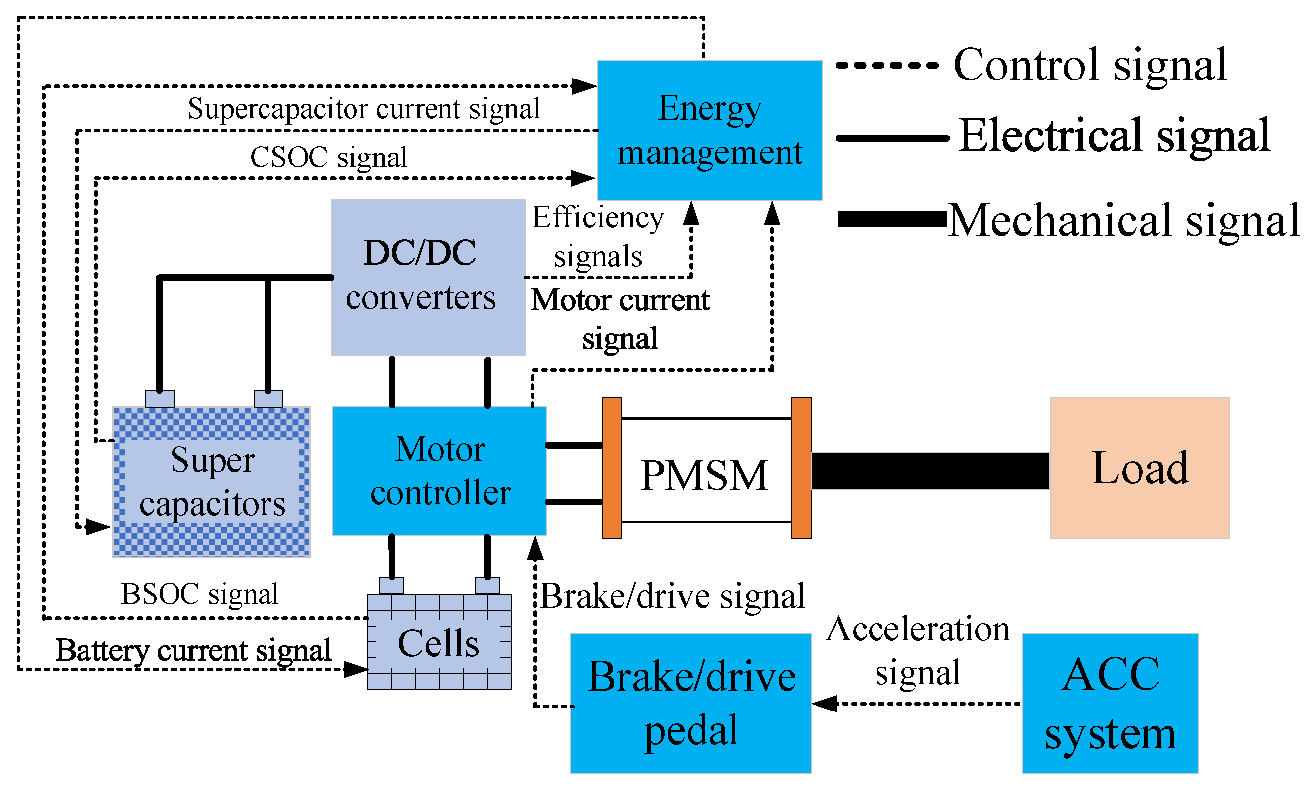
2.2. HESS Model

As illustrated in Figure 4, the HESS integrates a DC/DC converter with a supercapacitor to mitigate voltage sag caused by high discharge currents [24]. The ACC system directly outputs acceleration/deceleration commands to the pedal controller, which transmits throttle/brake signals to the motor controller for real-time current regulation. The EMS dynamically coordinates the supercapacitor SOC, battery SOC, and motor current profiles, thereby enabling adaptive power allocation between the supercapacitor and battery. During energy recovery, the DC/DC converter steps down the voltage of high-frequency transient power for efficient supercapacitor absorption, while the battery directly stores low-frequency steady-state energy. When the supercapacitor reaches its SOC limit, the transient power is redirected to the battery via the DC/DC converter, preventing battery degradation from high-frequency current pulses and minimizing voltage disparity-induced energy losses. The fundamental parameters delineated in

Table 1. Ego vehicle basic parameters.

Parameter Type	Parameter Name	Value
Whole vehicle	Curb weight/kg	1370
	Windward area/m2	2.4
	Rolling resistance coefficient	0.02
	Wind resistance	0.342
	Rotating mass conversion factor	1.05
	Tyre rolling radius/m	0.325
	Transmission efficiency	0.96
Motor	Rated speed/(r/min)	3000
	Maximum speed/(r/min)	9000
	Rated torque/(N.m)	88
	Maximum torque/(N.m)	264
	Peak power/kW	83
	Rated power/kW	46
Lithium-ion battery	Quantity	1
	Unit capacity/Ah	60
	Maximum voltage/V	349.6
	Minimum voltage/V	320
	Internal resistance/Ω	0.8
Supercapacitor	Quantity	4
	Peak voltage/V	432
	Minimum voltage/V	250
	Unit capacity/F	23.6
	Internal resistance/Ω	0.045
	DC/DC efficiency	0.9

encompass vehicle mass, electric motors, lithium-ion batteries, and supercapacitors, amongst other components.

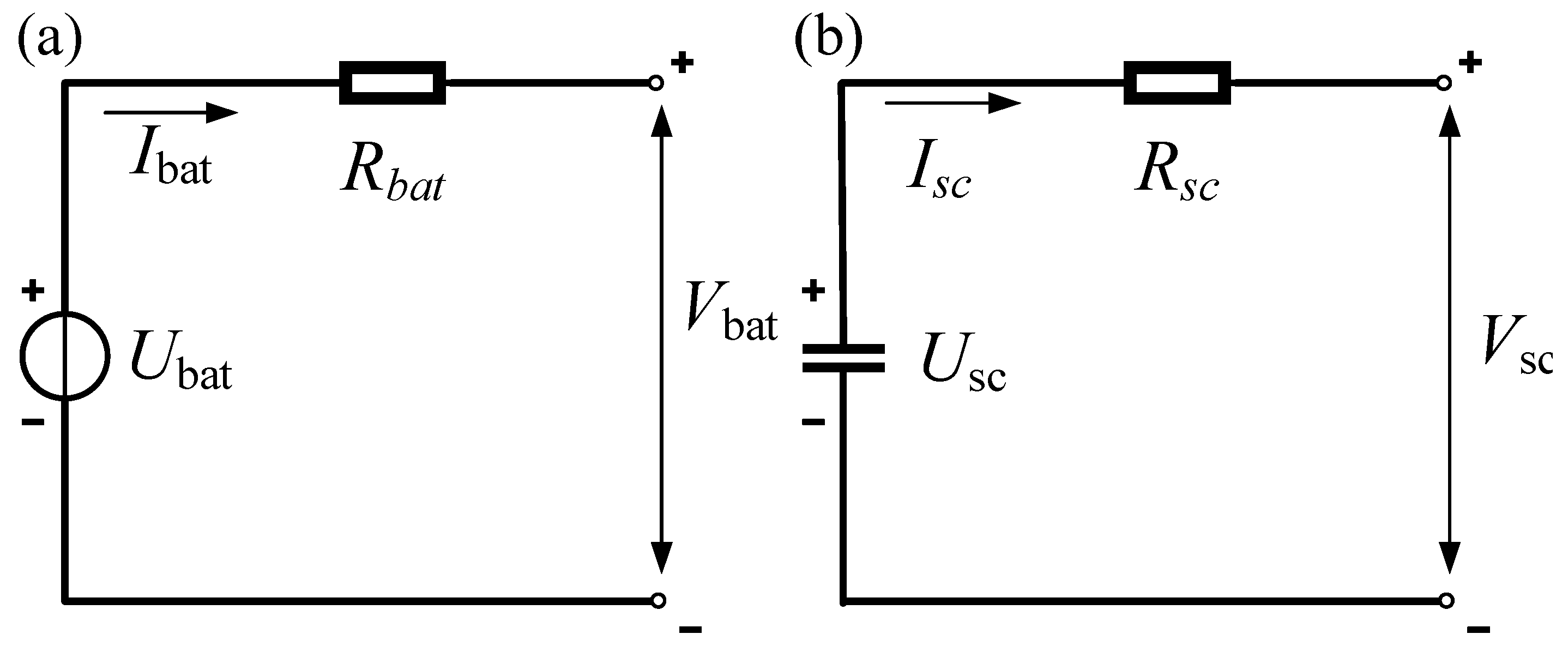
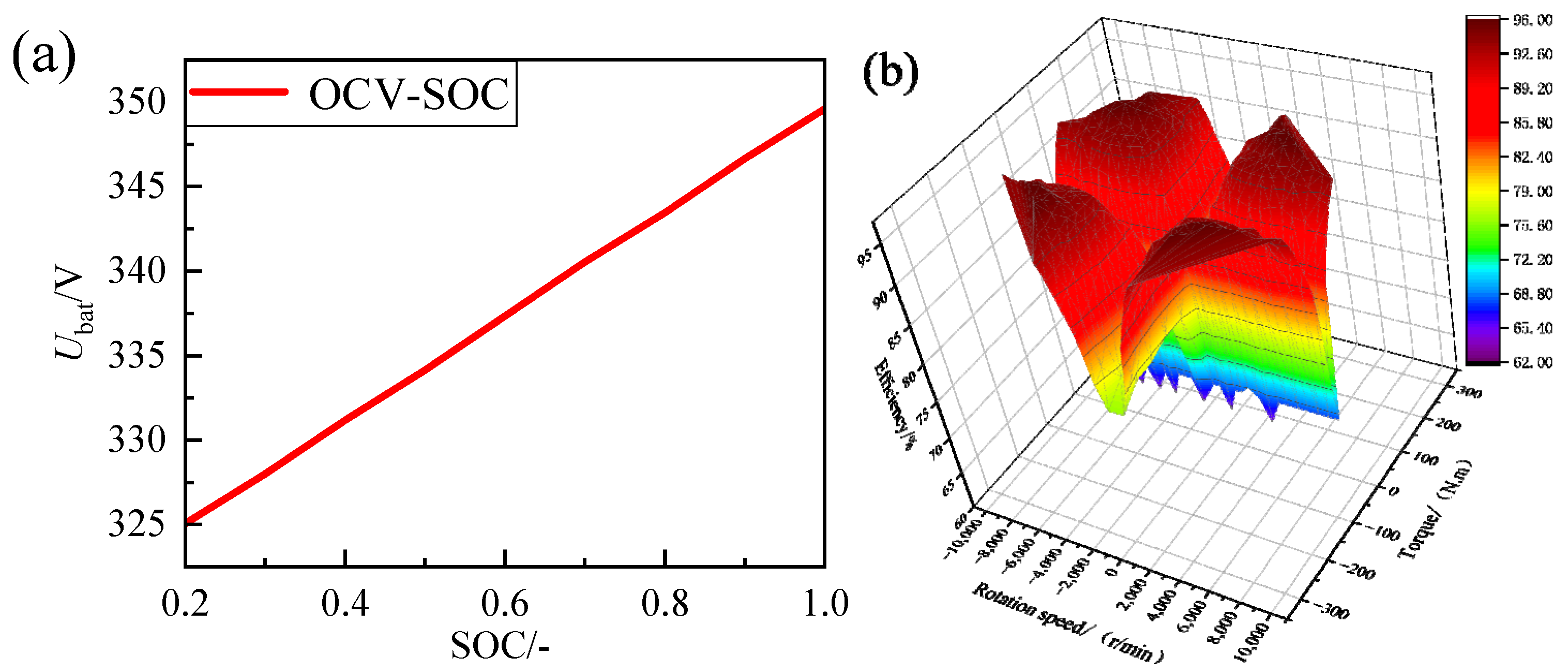
2.2.1. Lithium-Ion Battery Model

Lithium-ion batteries boast several advantages, including high energy density, rapid charging and discharging, and an extensive operating temperature range [25]. The modeling methods employed for lithium-ion batteries principally comprise neural networks [26,27,28], electrochemistry [29,30], and equivalent circuits [31,32,33], in addition to data-driven models [34,35,36,37]. The Rint equivalent circuit model (illustrated in Figure 5a) is notable for its ability to describe the change of external characteristics of the battery by using the circuit method, which is easy to control.

The Rint equivalent circuit is a theoretical model that does not consider the polarization reaction occurring within the battery. It consists of an ideal voltage source and a constant internal resistance connected in series. The open circuit voltage and charge state are illustrated in Figure 6a according to the equivalent circuit model of a lithium-ion battery as implemented in Cruise software. The expression for the battery current is as follows [31]:

$$I_{\mathrm{b}\mathrm{a}\mathrm{t}}={\displaystyle \frac{U_{\mathrm{b}\mathrm{a}\mathrm{t}}-\sqrt{U_{\mathrm{b}\mathrm{a}\mathrm{t}}^2-4P_{\mathrm{b}\mathrm{a}\mathrm{t}}{R}_{\mathrm{b}\mathrm{a}\mathrm{t}}}}{2R_{\mathrm{b}\mathrm{a}\mathrm{t}}}},$$

(7)

In the formula, U_bat represents the battery open-circuit voltage, I_bat denotes the current, R_bat stands for the equivalent internal resistance of the battery, and P_bat indicates battery power.

The charging and discharging efficiencies are expressed as follows:

$${\eta }_{\mathrm{b}\mathrm{a}\mathrm{t}}={\displaystyle \frac{U_{\mathrm{bat}}{I}_{\mathrm{bat}}-{I^2}_{\mathrm{bat}}{R}_{\mathrm{bat}}}{U_{\mathrm{bat}}{I}_{\mathrm{bat}}}},$$

(8)

Finally, the state of charge of the battery SOC is expressed as follows, in accordance with the definition thereof [16]:

$$\mathrm{S}\mathrm{O}{\mathrm{C}}_{\mathrm{bat}}(\mathrm{t})=\mathrm{S}\mathrm{O}{\mathrm{C}}_0{,}_{\mathrm{b}\mathrm{a}\mathrm{t}}-{\displaystyle \frac{{\displaystyle {\int }_0^t{I}_{\mathrm{b}\mathrm{a}\mathrm{t}}}\left(\mathrm{t}\right)\mathrm{d}\mathrm{t}}{{\eta }_{\mathrm{b}\mathrm{a}\mathrm{t}}{Q}_{\mathrm{i}\mathrm{n}\mathrm{i}\mathrm{t}}}},$$

(9)

In the formula, SOC_0,bat indicates the initial charge value of the lithium-ion battery; Q_init denotes the battery’s initial charge.

2.2.2. Supercapacitor Model

The high-power density of supercapacitors enables high-frequency energy release and storage, which can complement the advantages and disadvantages of lithium-ion batteries. The RC equivalent circuit is utilized to delineate the external characteristics of the supercapacitor, as illustrated in Figure 5b. The RC circuit consists of an equivalent internal resistance R_sc and a capacitor U_sc in series. According to Kirchhoff’s voltage law, the circuit terminal voltage V_sc can be expressed by the following equation:

$$V_{\mathrm{s}\mathrm{c}}=U_{\mathrm{s}\mathrm{c}}-I_{\mathrm{s}\mathrm{c}}{R}_{\mathrm{s}\mathrm{c}},$$

(10)

In the formula, V_sc represents the circuit voltage; U_sc stands for the open circuit voltage; I_sc denotes the current; R_sc signifies the equivalent internal resistance.

The supercapacitor circuit-terminal voltage can describe the change in charge. The expression for the supercapacitor state of charge (SOC_uc) is given below [17]:

$${\mathrm{SOC}}_{\mathrm{uc}}={\displaystyle \frac{V_{\mathrm{s}\mathrm{c}}-V_{\min }}{V_{\max }-V_{\min }}},$$

(11)

In the formula, V_min represents the maximum circuit voltage, and V_max stands for the minimum circuit voltage.

2.2.3. Motor Model

In this paper, the focus is on a permanent magnet synchronous motor, which has been selected for its ability to both drive the vehicle and facilitate energy recovery through braking. The relationship between motor power, torque, and speed is as follows:

$$P_{\mathrm{moter}}={\eta }_{\mathrm{moter}}{\displaystyle \frac{T_{\mathrm{moter}}{n}_{\mathrm{moter}}}{9550}},$$

(12)

In the formula, P_motor represents the motor power; T_motor stands for the motor torque; n_motor signifies the motor speed; η_motor denotes the motor efficiency, as illustrated in Figure 6b.

The vehicle travel equation is expressed as follows:

$${\displaystyle \frac{T_{\mathrm{moter}}{i}_0{\eta }_T}{r}}=mgf\cos \theta +mg\sin \theta +{\displaystyle \frac{C_{\mathrm{D}}A}{21.15}}{v}^2+\delta ma,$$

(13)

$$n_{\mathrm{motor}}={\displaystyle \frac{v{i}_0}{0.377r}},$$

(14)

In the formulas, i₀ represents the main gearbox ratio; η_T indicates the transmission efficiency; m denotes the vehicle mass; r stands for the tire rolling radius; θ represents the slope angle; C_D indicates the wind resistance coefficient; A denotes the windward area; v stands for the vehicle traveling speed; δ indicates the conversion factor of the rotating mass; g represents the gravitational acceleration; a stands for vehicle acceleration.

Curved-road adaptive cruise scenarios are excluded from consideration in this study. The longitudinal slope angle at time step k under straight-road conditions is defined as follows [38]:

$${\theta }_{\mathrm{k}}=\arcsin ({\displaystyle \frac{h{(s)}_{\mathrm{k}+1}-h{(s)}_{\mathrm{k}}}{s_{\mathrm{k}+1}-s_{\mathrm{k}}}}),$$

(15)

In the formula, h represents the vehicle traveling road height; s denotes the vehicle traveling road length. Road elevation h is retrieved via the Google Elevation API based on vehicle geolocation coordinates [39].

3. Design of Adaptive Cruise Algorithm Based on Vehicle Speed Prediction

3.1. Establishment of Multi-Objective Function

3.1.1. Longitudinal Tracking Performance

The ACC system prioritizes three operational objectives: vehicle-following precision, energy efficiency, and ride comfort. This study integrates the following performance and ride comfort metrics through weighted normalization, collectively defined as tracking quality optimization. Optimal tracking quality requires minimizing velocity differential (Δv) and inter-vehicle distance error (Δd), which are critical determinants of longitudinal collision risk. For ride comfort, acceleration is more easily measured relative to the jerk metric (time derivative of acceleration) and is responsive to the comfort of the vehicle [40]. Considering the optimal tracking quality and ride comfort of the whole prediction time domain, the longitudinal tracking performance is constructed by applying the two-paradigm number in the following equation:

$$\begin{array}{l}{J}_1={\displaystyle \sum {‖\Delta d(k+i|k)‖}_{q_1}^2}+{‖v_{\mathrm{rel}}(k+i|k)‖}_{q_2}^2+{‖a_{\mathrm{h}}(k+i|k)‖}_{q_3}^2\\ ={\displaystyle \sum {‖\mathit{y}(k+i|k)‖}_q^2},i=1,2\dots N_{\mathrm{p}}\end{array},$$

(16)

In the formula, N_p stands for the prediction time domain; q = $\left[\begin{array}{ccc}{q}_1& 0& 0\\ 0& q_2& 0\\ 0& 0& q_3\end{array}\right]$, q₁ and q₂ represent the optimal tracking quality weight coefficients, which take the values of 2 and 5 in this paper, respectively; q₃ indicates the ride comfort weight coefficient, which takes the value of 1 in this paper.

3.1.2. Energy Economy

In this paper, the driving power demand of vehicles is employed as an energy economic metric. The driving power demand of vehicles is summed in the prediction time domain as follows [41]:

$$J_2={\displaystyle \underset{k}{\overset{k+N_{\mathrm{p}}}{\int }}{P}_{\mathrm{req}}dt}={\displaystyle \underset{\mathrm{k}}{\overset{k+N_{\mathrm{p}}}{\int }}\frac{mgf{v}_h\cos \theta +mg{v}_h\sin \theta +C_{D}A{v_h}^3/21.15+\delta \mathrm{m}{a}_{\mathrm{h}}{v}_h}{{\eta }_T\times 9550\times 0.377}dt},$$

(17)

In the formula, P_req denotes the driving power demand of vehicles.

Assuming that the driving power demand of vehicles remains unchanged during the discrete time, the discrete expression for the total vehicle power demand in the predicted time domain is as follows:

$$\begin{array}{l}{J}_2={\displaystyle \sum P_{\mathrm{req}}}\times T\\ =T{\displaystyle \sum (\frac{mgf{v}_h(k+i|k)\cos \theta +mg{v}_h(k+i|k)\sin \theta }{{\eta }_T\times 9550\times 0.377}}+\dots \\ +{\displaystyle \frac{C_{D}A{v^3}_h(k+i|k)/21.15+\delta \mathrm{m}{a}_{\mathrm{h}}(k+i|k)v_h(k+i|k)}{{\eta }_T\times 9550\times 0.377}}), i=1,2\cdots N_{\mathrm{p}}\end{array},$$

(18)

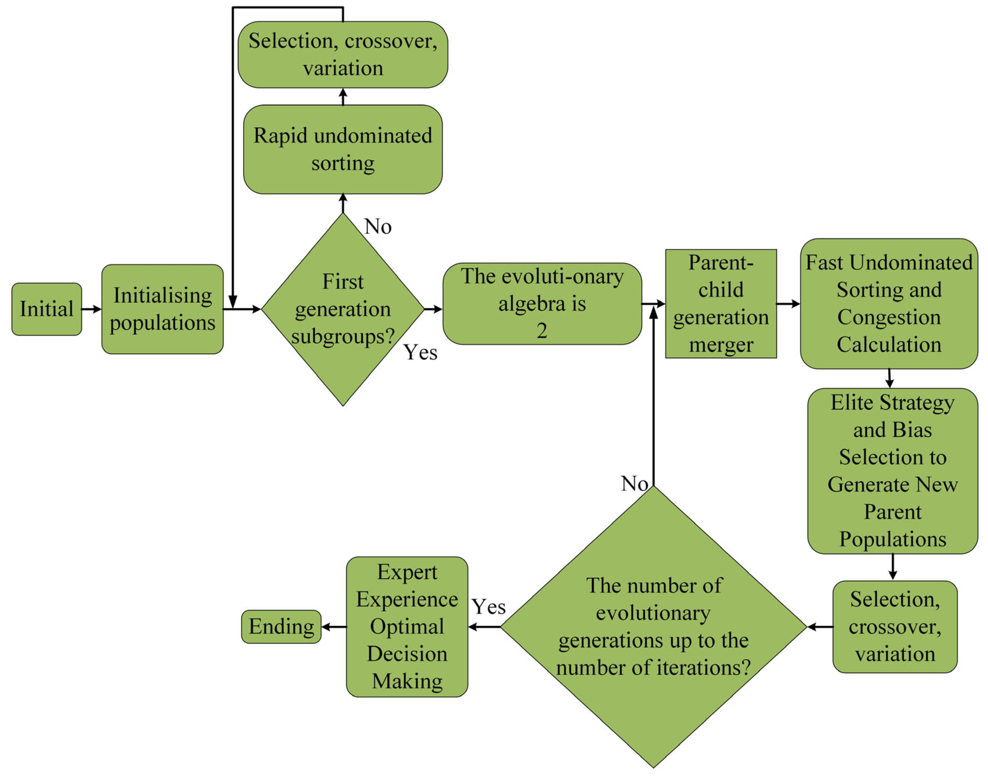
3.2. Fast Non-Dominated Sorting Genetic Algorithm NSGA-II Optimisation Solution

The performance objectives derived in Section 2.1 are then linearly superimposed to form a multi-objective function with constraints on ∆v, ∆d, and a_h:

$$\begin{array}{l}\min J=J_1+J_2={\displaystyle \sum {‖y(k+i|k)‖}_q^2}+{\displaystyle \underset{k}{\overset{k+N_{\mathrm{p}}}{\int }}{P}_{\mathrm{req}}dt}\\ s.t\left\{\begin{array}{l}\Delta v_{\min }\le \Delta v(k+i|k)\le \Delta v_{\max }\\ a_{\mathrm{h},\min }\le a_h(k+i|k)\le a_{\mathrm{h},\max }\\ a_{\mathrm{des},\min }\le a_{\mathrm{des}}(k+i)\le a_{\mathrm{des},\max }\\ d(k+i|k)-d_{\mathrm{des},\max }\le \Delta d(k+i|k)\le d(k+i|k)-d_{\mathrm{des},\min }\\ i=1,2\cdots N_{\mathrm{p}}\end{array}\right.\end{array},$$

(19)

In the formula, Δv_min represents the relative speed minimum, which takes the value of −4 in this paper; Δv_max stands for the relative speed maximum value, which takes the value of 4 in this paper; a_h,min signifies the acceleration minimum value, which takes the value of −3 m/s² in this paper; a_h,max denotes the acceleration maximum value, which takes the value of 2 m/s² in this paper; a_des,min indicates the expected acceleration minimum value, which takes the value of −3 m/s² in this paper; a_des,max represents the expected acceleration maximum value, which takes the value of 2 m/s² in this paper; d_des,max signifies the upper limit of the desired distance; d_des,min indicates the upper limit of the desired distance; the limit of the desired distance determined by Figure 2.

J is defined as a two-dimensional objective function, while the constraints are represented as linear inequalities, suitable for solving the desired acceleration sequence U(k + Np) = { a_{des, k}, a_des,k+1, …, a_des,k+Np} by applying the NSGA-II. NSGA-II introduces the concept of a Pareto non-dominated solution set on the basis of a genetic algorithm. The algorithm is comprised of three parts: fast non-dominated sorting, congestion calculation and elite retention strategy. These additions greatly reduce the arithmetic complexity of the genetic algorithm [42].

3.2.1. Fast Non-Dominated Sorting

It is hypothesized that two solutions exist, i.e., U₁ and U₂, which satisfy equation 20. It is further postulated that U₁ dominates U₂. A set of solutions is said to be non-dominated if there is no mutual dominance between the solutions in the set.

$$\left\{\begin{array}{l}{J}_{\mathrm{i}}(U_1)\le J_{\mathrm{i}}(U_2),\forall \mathrm{i}\in 1,2\\ J_{\mathrm{j}}(U_1)<J_{\mathrm{j}}(U_2),\exists \mathrm{j}\in 1,2\end{array}\right.,$$

(20)

Following a series of operations including, but not limited to, hybridization, mutation, and selection, a set of populations, that is to say, solutions, will be obtained. The first set of non-dominated sorted solution sets will then be screened and assigned a rank of 1. The remaining candidate solutions are iteratively filtered through identical dominance criteria and assigned hierarchical ranking indices until exhaustive classification. This hierarchical stratification process is formally defined as non-dominated sorting in evolutionary multi-objective optimization frameworks. The fast, non-dominated sorting method has been shown to reduce the time complexity from O(mN³) to O(mN²) based on the non-dominated sorting method. This reduction in complexity can be achieved through the following steps:

The individual parameter n_q is defined as the number of dominant individuals q in the population, and S_q is defined as the set of individuals dominated by individual q. It should be noted that q = 1, …, N, where N is the population size.

Step 1: A non-dominated sorting judgment is to be performed on all individuals within the population, with the values of all individual parameters (n_q, S_q) subsequently being calculated.

Step 2: The identification of individuals in the population with n_q = 0 is the first step. These individuals are then assigned a non-dominated rank of 1. The next step is to deposit the individuals in the non-dominated set, rank1.

Step 3: The process of subtraction of 1 from n_q for each individual in the set S_q of all individuals in the set rank1 corresponding to the dominated individuals is to be carried out. In the event of n_q − 1 = 0, the individual is to be stored as in the set rank2 and assigned the domination rank 2.

Step 4: Repeat the above for the individuals in rank 2 until all individuals are assigned non-dominated ranks.

3.2.2. Crowding Distance and Bias Sequence

The concept of crowding distance is defined as the degree of aggregation of individuals within the same non-dominated class. The crowding distance of individual j on the ith target J_i (i = 1, 2) is expressed as follows:

$$d_{\mathrm{j}}={\displaystyle \sum \left|{J_{\mathrm{i}}}^{\mathrm{j}+1}-{J_{\mathrm{i}}}^{\mathrm{j}-1}\right|},$$

(21)

In the formula, d_j denotes the crowding distance of individual j.

In order to select the optimal individual, based on the non-dominated ordering hierarchy and the congestion distance, for any individual U_i and U_j, the following definition is proposed: U_i is to be biased over U_j:

$$\begin{array}{c}{U}_{\mathrm{i}}{\prec }_n{U}_{\mathrm{j}}\\ if\left[(U_{\mathrm{i},\mathrm{r}\mathrm{a}\mathrm{n}\mathrm{k}}<U_{\mathrm{j},\mathrm{r}\mathrm{a}\mathrm{n}\mathrm{k}})or(U_{\mathrm{i},\mathrm{r}\mathrm{a}\mathrm{n}\mathrm{k}}=U_{\mathrm{j},\mathrm{r}\mathrm{a}\mathrm{n}\mathrm{k}}and{U}_{\mathrm{i},\mathrm{d}}<U_{\mathrm{j},\mathrm{d}})\right]\end{array},$$

(22)

In the formula, U_i,rank and U_j,rank denote the non-dominance rank of individuals U_i and U_j, respectively; U_i,d, and U_j,d represent the crowding distance of individuals U_i and U_j, respectively.

3.2.3. Elite Selection Strategy

The elite preservation mechanism combines the parent population (P_t) and offspring population (Q_t) into an extended candidate pool (R_t). This merged population attains a cardinality of 2N individuals, where N represents the baseline population size in evolutionary optimization algorithms. This process serves to expand the screening range of the subsequent generation and enhance the diversity of the population. The selection process is delineated in Figure 7 and comprises the following steps:

Step 1: A fast non-dominated sort is to be performed on the new population R_t in order to form n non-dominated sorted sets.

Step 2: The non-dominated sorted collection is then to be placed into the new parent by sorting rank.

Step 3: Individuals in rank k with partial ordering positions exceeding N−N_k−1 and those possessing non-dominated sorting ranks inferior to k are systematically pruned. This elimination protocol generates the authentic parent population P_t+1 through dominance-based stratification.

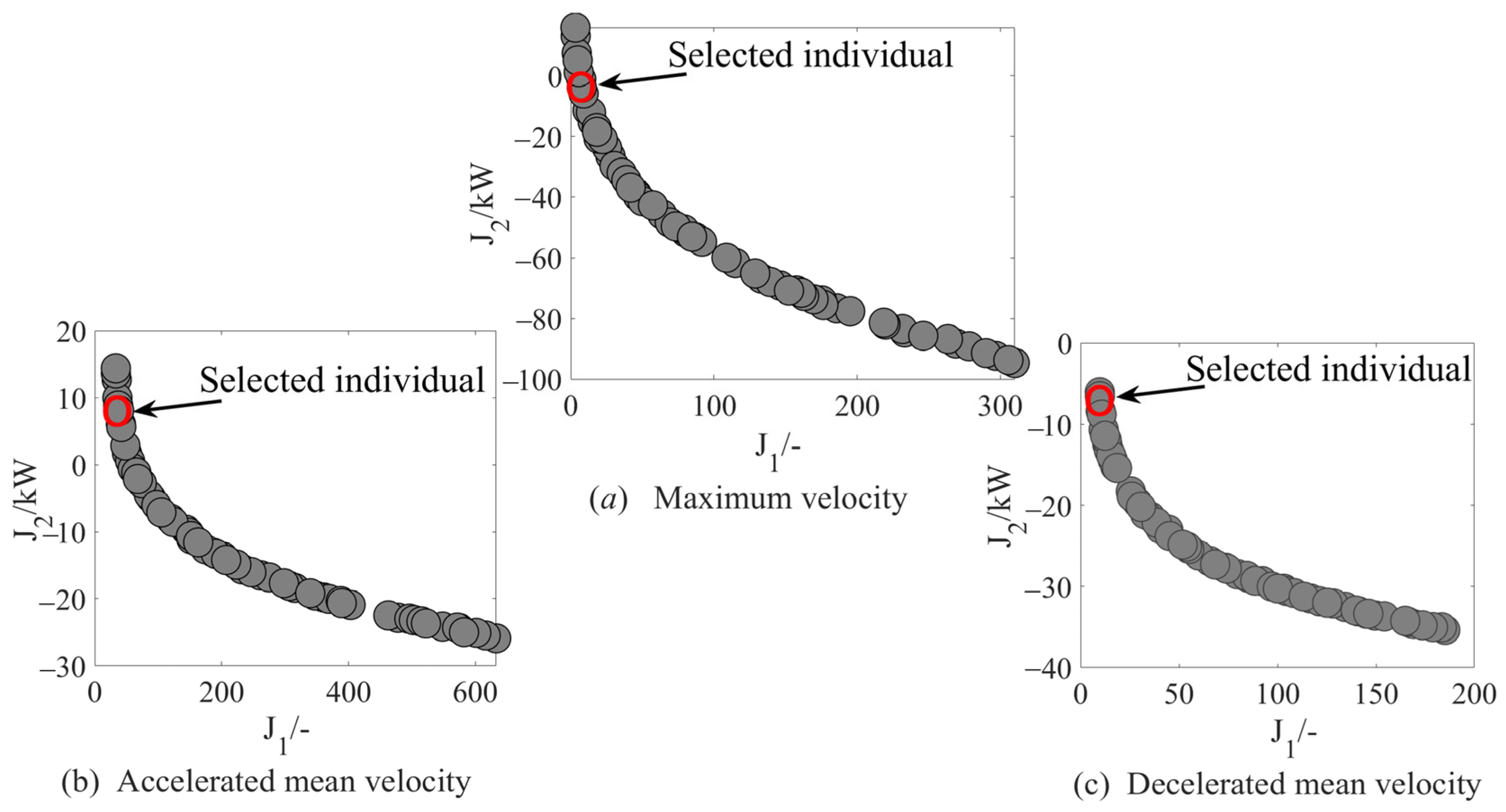
3.2.4. Optimal Individual Decision

The objective function J is solved using NSGA-II to obtain the optimal Pareto front, i.e., a set of non-dominated optimal solution sets. It is evident that the solutions constituting the set of undominated optimal solutions are not mutually exclusive, and thus, they cannot be selected directly. The optimal solution that is sought must, therefore, be selected through the utilization of expert experience. In order to determine the optimal solution policy rule, the following requirements must be taken into consideration:

(1)

The time-domain predicted power demand must be constrained below the motor’s peak power output capacity throughout the driving cycle. This critical operational constraint guarantees the electric machine’s dynamic response capability to deliver the required tractive effort.

(2)

The primary concern is the capacity for longitudinal tracking performance, a matter that is addressed through a combination of energy economy considerations.

In consideration of the aforementioned requirements, the optimal solution policy rule is hereby defined as follows:

Step 1: In accordance with requirement 1, set H₁ is comprised of the liberation that satisfies equation 23. The set H₁ is then sorted according to J₁, with the top 10% being extracted into the set H₂.

$$P_{\mathrm{req},\mathrm{k}+\mathrm{i}|\mathrm{k}}(v_{\mathrm{k}+\mathrm{i}|\mathrm{k}},a_{\mathrm{k}+\mathrm{i}|\mathrm{k}})\le P_{\mathrm{motor},\mathrm{peak}},i=1\cdots N_{\mathrm{p}},$$

(23)

In the formula, P_req,k+i|k denotes the demand power at moment k predicted at moment k + i and P_motor,peak stands for the peak power of the motor.

Step2: In H₂, the solutions are evaluated in a comprehensive manner, with each solution satisfying the criteria outlined in Equation (24). The solution that achieves the maximum score is then identified as the optimal solution and is designated U_best.

$$grad{e}_{\mathrm{i}}={\displaystyle \frac{J_{1,\min }}{J_{1,\mathrm{i}}}}+{\displaystyle \frac{J_{2,\min }}{J_{2,\mathrm{i}}}} ,i=1\cdots M,$$

(24)

In the formula, grade_i denotes the total score of the ith solution; J_1,min and J_2,min denote the optimal following and economy in the set H₂, respectively; J_1,i and J_2,i represent the following and economy of the ith solution, respectively; M signifies the number of solutions in the set H₂.

Finally, in this paper, the algorithmic parameters are configured as: population size 200, maximum generations 200, crossover probability 0.8, mutation probability 0.2, and elitism preservation rate 0.05. The NSGA-II solution workflow implementing these operators (selection, crossover, mutation) with crowding distance-based niching is systematically illustrated in Figure 8.

4. Design of Energy Management Strategy for HESS

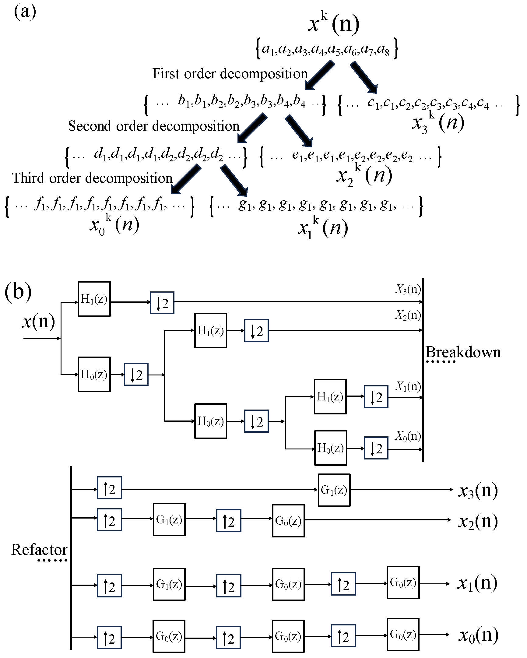
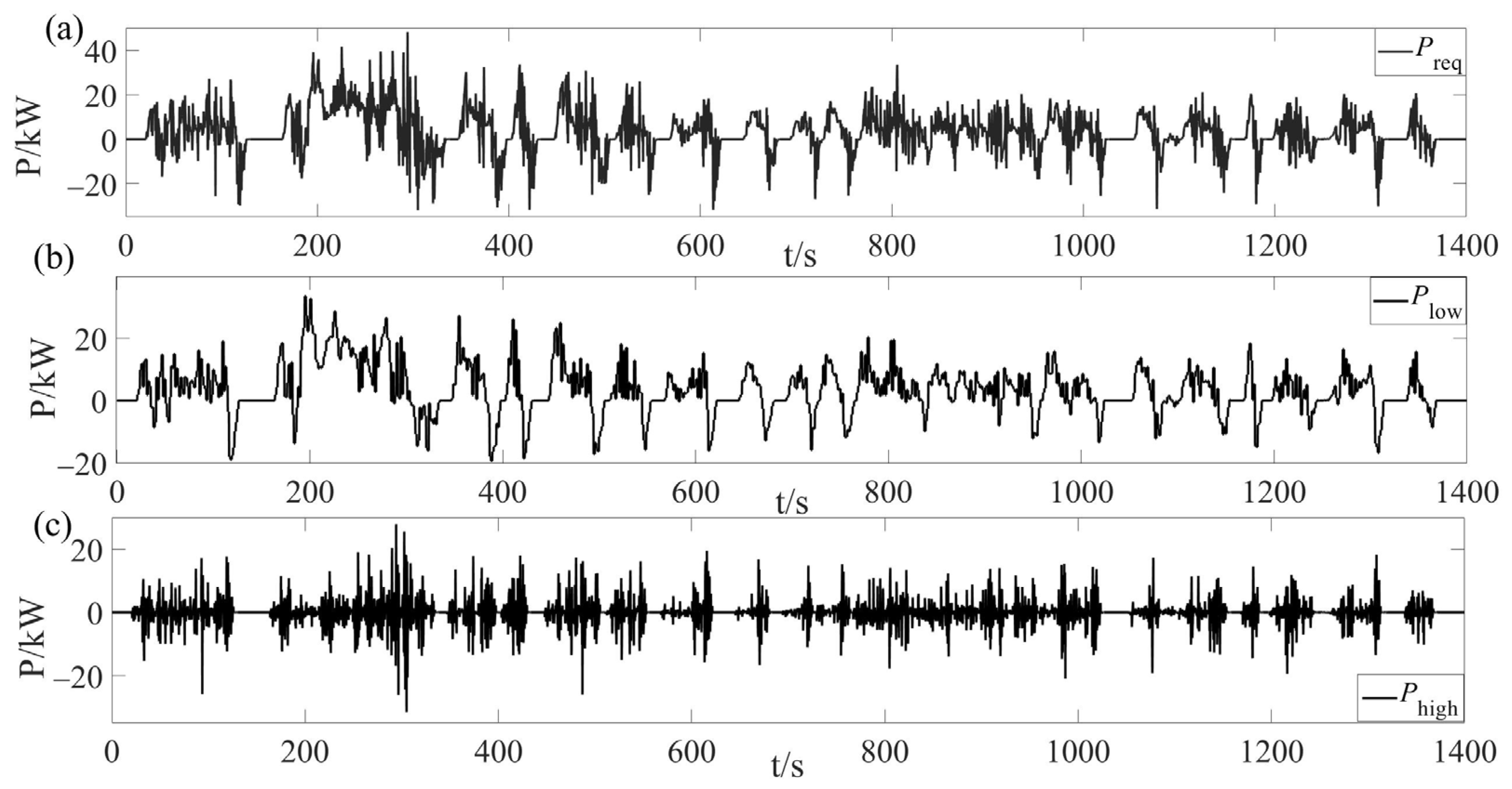
4.1. Haar Wavelet Decomposition of Demand Power

The Haar wavelet demonstrates superior computational efficiency in demand power time-frequency decomposition compared to other wavelets. This structural advantage stems from its minimal-length finite impulse response filter and symmetrical filter architecture, which enables identical forward/inverse transformation coefficients. The Harr wavelet mother function is given in the following equation:

$$\psi (t)=\left\{\begin{array}{cc}1& t\in \left[0,1/2\right]\\ -1& t\in \left[1/2,1\right]\\ 0& \mathrm{other}\end{array}\right.,$$

(25)

Third-order Haar wavelets have been demonstrated to be appropriate for demand power decomposition due to their computational efficiency and the satisfactory quality of the decomposition results [13]. The online decomposition of demand power utilizes the third-order Haar wavelet, requiring seven moments of demand power in addition to the current moment. Consequently, the prediction time domain of the follow-me algorithm is N_p = 7, as illustrated in Figure 9a below. The three-level Haar wavelet decomposition-reconstruction architecture employs high-pass and low-pass filters defined as [H₁(z),H₀(z)]^T and [G₁(z),G₀(z)]^T, respectively. This hierarchical filter bank implements dyadic downsampling (decimation factor = 2) during decomposition and symmetrical upsampling (interpolation factor = 2) during reconstruction, thereby preserving time-frequency energy equivalence across all decomposition levels. The decomposition and reconstruction process is shown in Figure 9b as follows. The decomposition and reconstruction filter banks satisfy the orthogonality condition with the following equation [43]:

$$\begin{array}{l}{[H_1(z)H_0(z)]}^{\mathrm{T}}={\displaystyle \frac{1}{2}}{[1-z^{-1}1+z^{-1}]}^{\mathrm{T}}\\ {[G_1(z)G_0(z)]}^{\mathrm{T}}={[1+z^{-1}1-z^{-1}]}^{\mathrm{T}}\end{array},$$

(26)

As illustrated in Figure 9a, the demand power of the signals x^k(n) prior to the decomposition exhibits variation in the kth prediction time domain. However, the demand power of the signals x₀^k(n) subsequent to three decompositions remains uniform, thereby ensuring a more uniform demand power profile. As illustrated in Figure 9b, the original signal x(n) is decomposed into X₃(n), X₂(n), X₁(n), X₀(n) by the filter [H₁(z), H₀(z)]^T. Subsequent to the second sampling, the signal’s length is reduced to L₃ = 4, L₂ = 2, L₁ = 1, L₀ = 1, respectively. In the course of the reconstruction process, the signals X₃(n), X₂(n), X₁(n), X₀(n) are reconstructed into X₃(n), X₂(n), X₁(n), X₀(n) through the filters [G₁(z), G₀(z)]^T. The length of the reconstructed signals after the upsampling is restored to the length of the original signals, L₃ = L₂ = L₁ = L₀ = 8, respectively. The final expression for the low-frequency power P_low and the high-frequency power P_high is as follows:

$$\begin{array}{l}{P}_{\mathrm{low}}(k+i|k)={x_0}^{\mathrm{k}}(n),i=1\dots 8\\ P_{\mathrm{high}}(k+i|k)={x_1}^{\mathrm{k}}(n)+{x_2}^{\mathrm{k}}(n)+{x_3}^{\mathrm{k}}(n)\\ \end{array},$$

(27)

Finally, this paper completes the framework construction of the ACC-WT algorithm. The pseudocode is shown in Algorithm 1. The algorithm inputs include ego vehicle velocity, front vehicle velocity, accelerations, and inter-vehicle distance. Its outputs are high-frequency transient demand power and low-frequency steady-state demand power. Initial weight coefficients and vehicle parameters are first initialized. A constrained car-following system cost function is then optimized using the NSGA-II algorithm. This optimization involves population screening, non-dominated sorting, crowding distance calculation, and Pareto frontier selection. The optimal solution is determined through power constraints and a scoring formula. This generates a demand power sequence for 3-level Haar wavelet decomposition. The proposed algorithm adapts prediction horizons via wavelet order, decoupling cruise demand power into transient and steady-state components.

Algorithm 1: ACC-WT Hierarchical Control Algorithm

Input: Ego vehicle: vh, ah   Front vehicle: vp, ap     Vehicle distance: d   Output: Power Components: Phigh, Plow   1: Initialize weight vector q1, q2, q3   Initialize ego vehicle parameters   2: Define cost functions and constraints   3: // ====== NSGA-II Optimization ======   4: Generate P₀ ← Random population (size=200)   5: for gen ← 1 to 200 do:   6:   Apply genetic operators:   Simulated binary crossover (η = 0.8)   Polynomial mutation (pm = 0.2)   7:   Fast non-dominated sorting → {rank1, …, rankn}   8:   Calculate crowding distance dj and bias sequence   9:  Select Pt+1 using Elite selection strategy   10: end for   11: // ====== Optimal individual decision ======    12: H₁ ← { U∈ P200 | Preq ≤ Pmotor,peak}   13: H₂ ← Top 10% solutions in H₁ by J₁   14: Compute score:   gradei = (J₁,min/J₁,i) + (J2,min/J2,i)   15: Ubest(k + Np) ← max(gradei)   16: // ====== Online Haar Decomposition ======    17: Preq = {Preq,k, Preq,k+1, …, Preq,k+7} ← Vehicle driving power calculation   18: [Phigh, Plow] ← 3-level Haar(Preq)   Decomposition: H₁(z) = 0.5(1 − z−1), H₀(z) = 0.5(1 + z−1) Reconstruction: G₁(z) = (1 + z−1), G₀(z) = (1 − z−1)

4.2. Low-Frequency Steady-State Power Quadratic Optimal Decomposition Based on Fuzzy Logic Control

The low-frequency demand power decomposition is conducted through quadratic optimization based on expert experience. This process aims to realize more optimal demand power allocation for vehicle adaptive cruise control. The power allocation factor is defined as follows:

$$K_{\mathrm{bat}}={\displaystyle \frac{P_{\mathrm{bat}}}{P_{\mathrm{low}}}},$$

(28)

In the formula, P_bat is the matched power of a lithium-ion battery, and K_bat signifies the power allocation factor.

The power output of the supercapacitor can be calculated using the following equation:

$$P_{\mathrm{uc}}=P_{\mathrm{high}}+(1-K_{\mathrm{bat}})P_{\mathrm{low}},$$

(29)

In the formula, P_uc is the matched power of a supercapacitor.

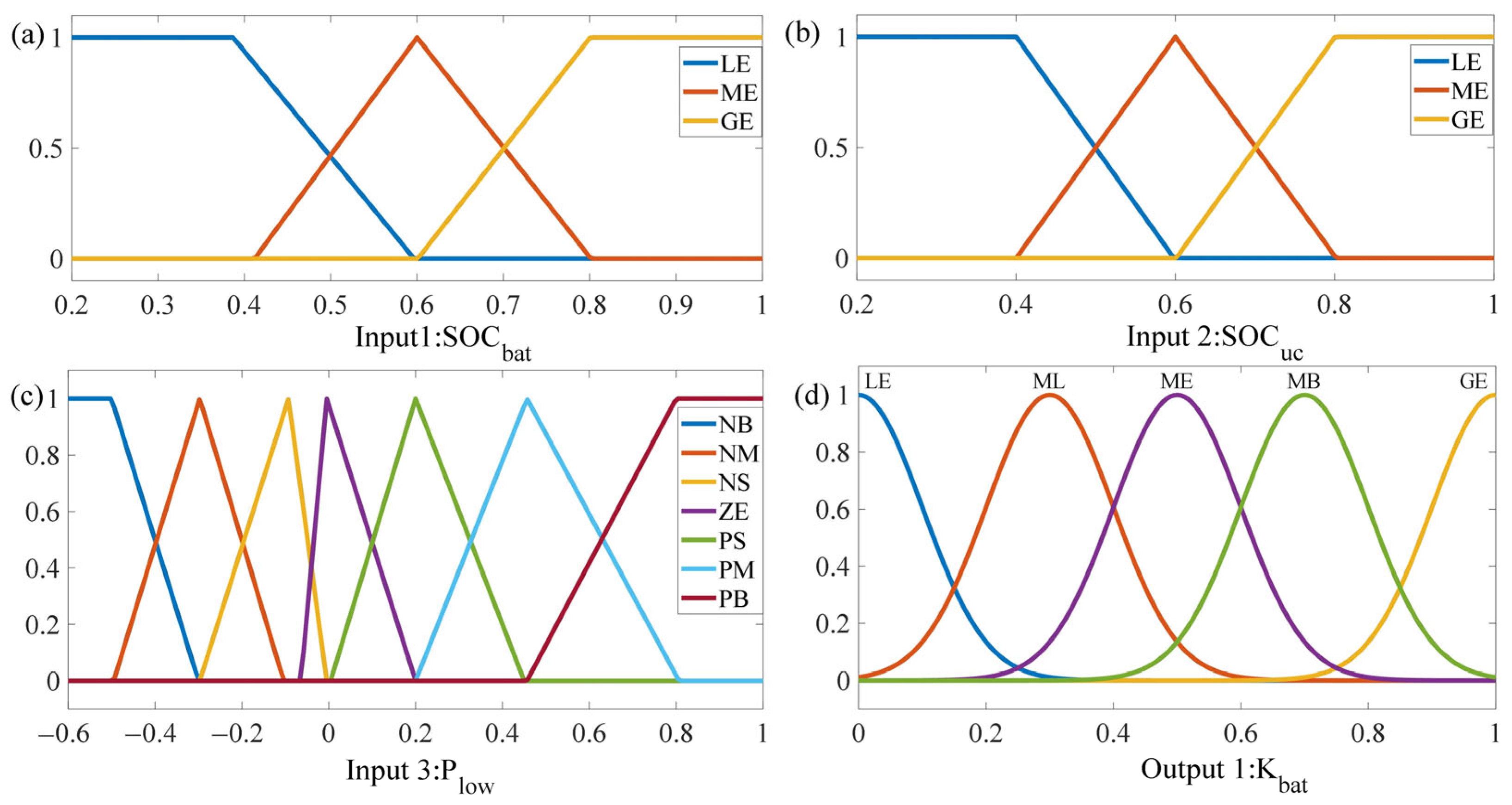
4.2.1. Control Variable Setting and Fuzzy Subset Delineation

Fuzzy logic control demonstrates robustness and the ability to adapt to complex changes in operating conditions [44]. The inputs of the fuzzy control system are hereby defined as P_low, SOC_bat, and SOC_uc, with the power allocation factor K_bat serving as the system’s output. It is acknowledged that the demand power during braking is less than the motor’s maximum capacity. Therefore, the P_low thesis domain is established as [−0.6, 1], and the fuzzy subsets are categorized as P_low = [NB NM NS ZE PS PM PB]. When the battery’s state of charge falls below 0.2, the internal resistance of the battery is increased, thereby reducing the efficiency of charging and discharging. Consequently, the SOC_bat and SOC_uc domains are set to [0.2,1], and the fuzzy subsets are classified as SOC_bat = [LE ME GE] and SOC_uc = [LE ME GE]. The K_bat domain is set to [0,1], and the fuzzy subsets are classified as K_bat = [LE ML ME MB GE].

4.2.2. Control Variable Affiliation Function Design

The configuration of the affiliation function curve exerts a substantial influence on the efficacy of the fuzzy controller. A steep curve renders the controller responsive, while a flat curve renders the controller unresponsive. The low-frequency demand power P_low, lithium-ion battery SOC_bat, and supercapacitor SOC_uc select triangular and trapezoidal affiliation functions that respond quickly and are simple to compute. Accurate control of the power allocation factor K_bat is critically required. This necessitates the adoption of Gaussian-type affiliation functions with high computational precision to enhance the allocation factor’s accuracy. The affiliation function of the input and output variables of the fuzzy logic controller is illustrated in Figure 10.

4.2.3. Fuzzy Rule Design

The subsequent step involves the development of a rule table based on fuzzy principles, as shown in

Table 2. Fuzzy logic rules table.

Kbat	Plow
		NB	NM	NS	ZE	PS	PM	PB
SOCbat SOCuc = LE	LE	ML	ML	GE	GE	ME	ME	ML
	ME	LE	LE	LE	GE	GE	MB	MB
	GE	LE	LE	LE	GE	GE	MB	GE
SOCbat SOCuc = ME	LE	ML	ME	GE	GE	ME	ML	ML
	ME	LE	LE	LE	GE	GE	ME	LE
	GE	LE	LE	LE	GE	GE	ME	ML
SOCbat SOCuc = GE	LE	GE	GE	GE	GE	ML	LE	LE
	ME	MB	MB	ML	GE	GE	ML	LE
	GE	LE	LE	LE	GE	GE	ME	LE

below:

The following fuzzy principle is defined in accordance with the characteristics of supercapacitors and lithium-ion batteries:

(1)

In circumstances where demand power is minimal, the demand power is matched by the lithium-ion battery.

(2)

Under moderate traction power demand conditions, the lithium-ion battery exclusively handles the power demand when its SOC_bat is sufficiently high, regardless of the supercapacitor’s SOC_uc. Conversely, If SOC_bat is relatively low, coordinated power allocation between the supercapacitor and lithium-ion battery is activated to fulfill the operational requirements.

(3)

During high traction power demand, the supercapacitor solely supplies power when its SOC_uc is sufficient, independent of the lithium-ion battery’s SOC_bat. When SOC_uc becomes insufficient, both energy storage units jointly provide power to meet the demand.

(4)

Under braking conditions, the supercapacitor recycles the energy converted from larger and medium braking power. The lithium-ion battery recycles the energy converted from smaller braking power.

5. Simulation Verification

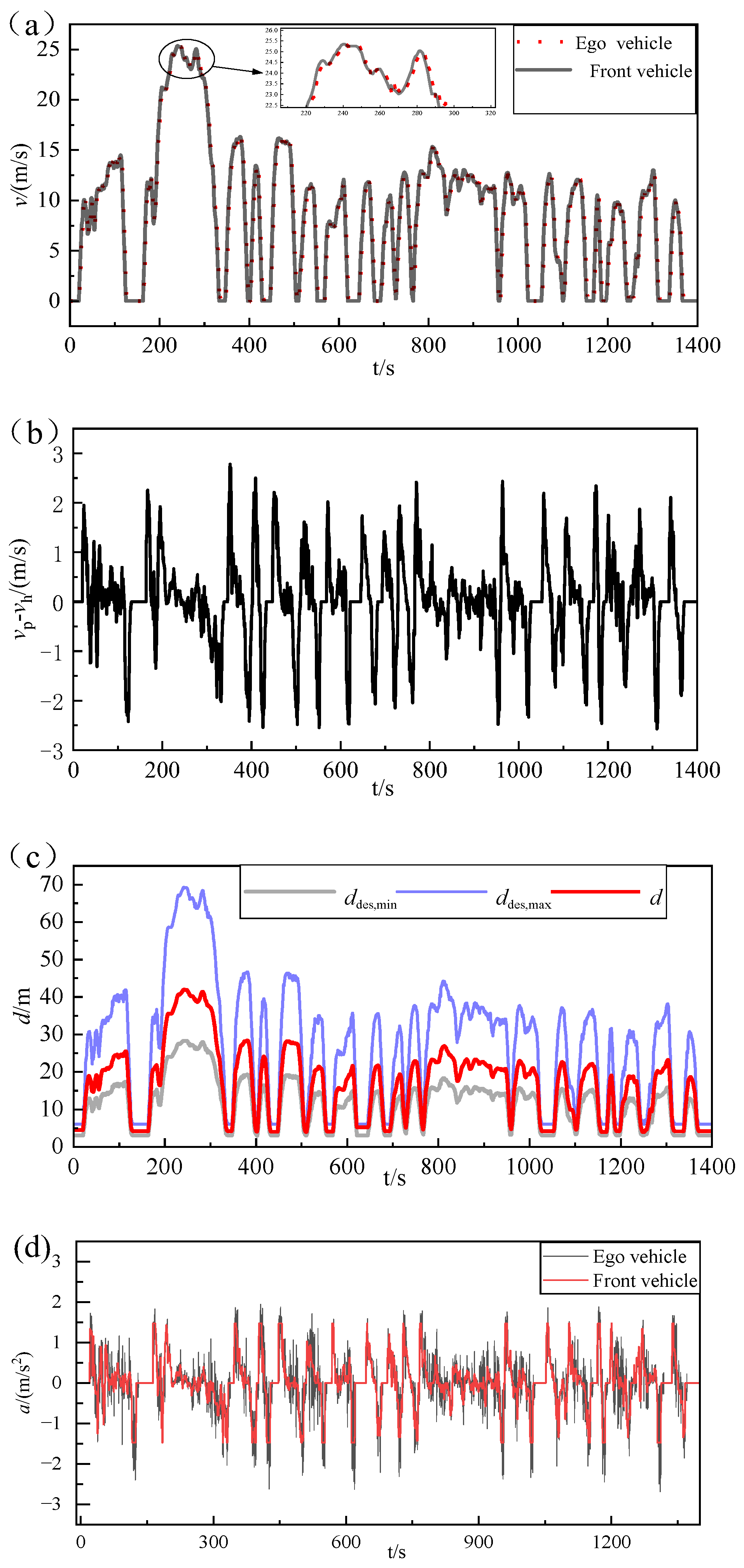
5.1. Simulation Verification of Followership Algorithm

This study employs MATLAB/Simulink to simulate and validate an ACC algorithm and EMS. The validation protocol adheres to the Urban Dynamometer Driving Schedule (UDDS), representing standardized urban driving conditions. The simulation sampling spacing T is set at 0.2 s, and the fundamental parameters of the entire vehicle are equivalent between the front vehicle and the ego vehicle. As illustrated in Figure 11a–c, the Pareto solution set at the highest and average speed of the front vehicle is demonstrated. The three cases exhibit analogous trends, indicating an inverse proportionality relationship. The selected individual changes in accordance with the working conditions, and J₁ is superior to J₂, which is consistent with the principle of the design of the individual selection.

Figure 12a,b, and

Table 3. Statistical table of follow-through data.

Parameter	Δv/(m/s)	d/m	a/(m/s2)
Maximum values	2.7	41.95	1.94
Minimum value	−2.57	3.97	−2.67
Average value	0.56	16.92	-

demonstrate that when the leading vehicle decelerates from its maximum speed of 25.347 m/s at 353 s, the instantaneous relative speed peaks at 2.7 m/s. The average relative speed throughout the driving cycle remains 0.5593 m/s, validating the stability of the car-following control strategy. As can be seen from Figure 12c, when both vehicles are parked, the upper limit of the desired distance is 6 m, and the lower limit of the desired distance is 3 m. Beyond the initial parking phase, subsequent parking conditions arise because the distance error fails to converge to zero, resulting in the relative distance not reaching the target of 4.5 m. Nevertheless, the error magnitude remains minimal, maintaining the relative distance within the predefined acceptable vehicle spacing range. Figure 12d demonstrates that under driving conditions, the maximum accelerations of the ego vehicle and front vehicle are 1.94 m/s² and 1.48 m/s², respectively. In braking scenarios, the maximum decelerations for both vehicles are recorded as −2.67 m/s² and −1.48 m/s².

As illustrated in Figure 13a, the total demanded power of the ego and front-vehicles is 4632 kW and 4811 kW, respectively. This represents a 3.71% decrease. As demonstrated in Figure 13b, the initial SOC of the single-source and HESS battery is 0.8. The final SOC of the single-source and HESS are 0.72339 and 0.74, respectively. This indicates an increase of 2.3% in SOC, suggesting a more gradual decline in the SOC of the HESS battery.

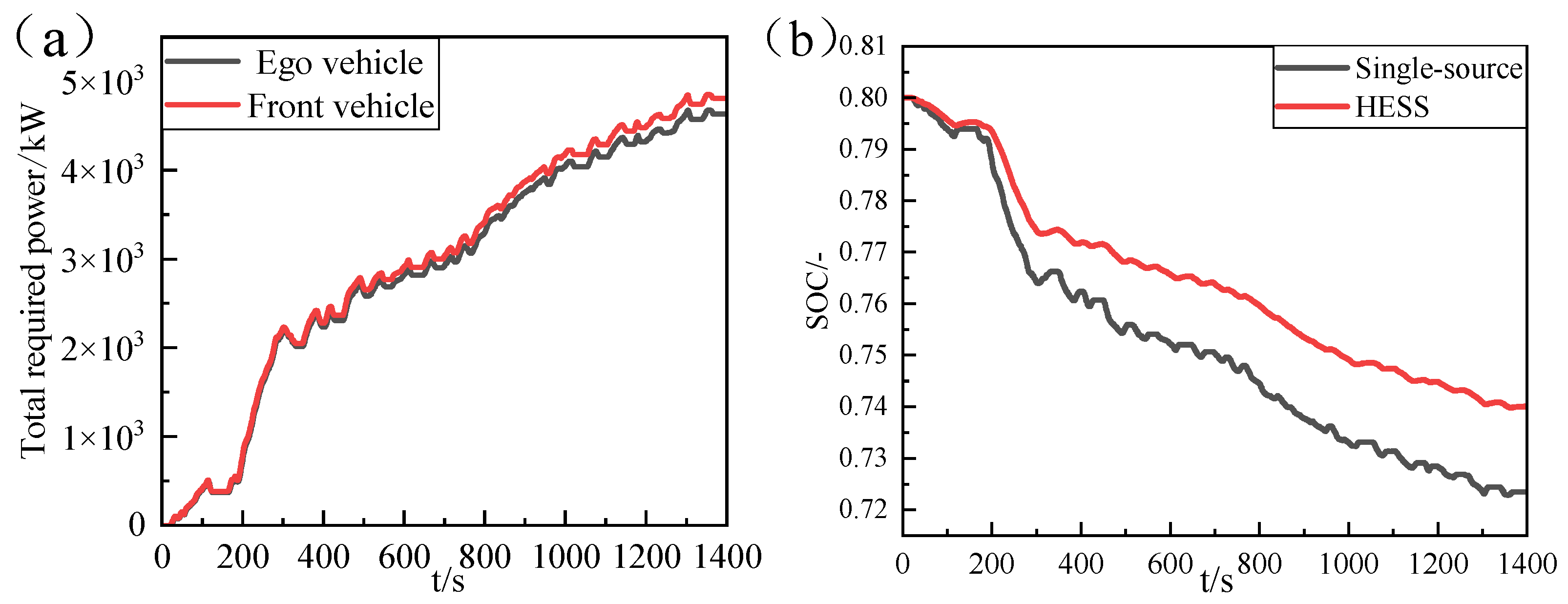
5.2. Simulation Verification of EMS

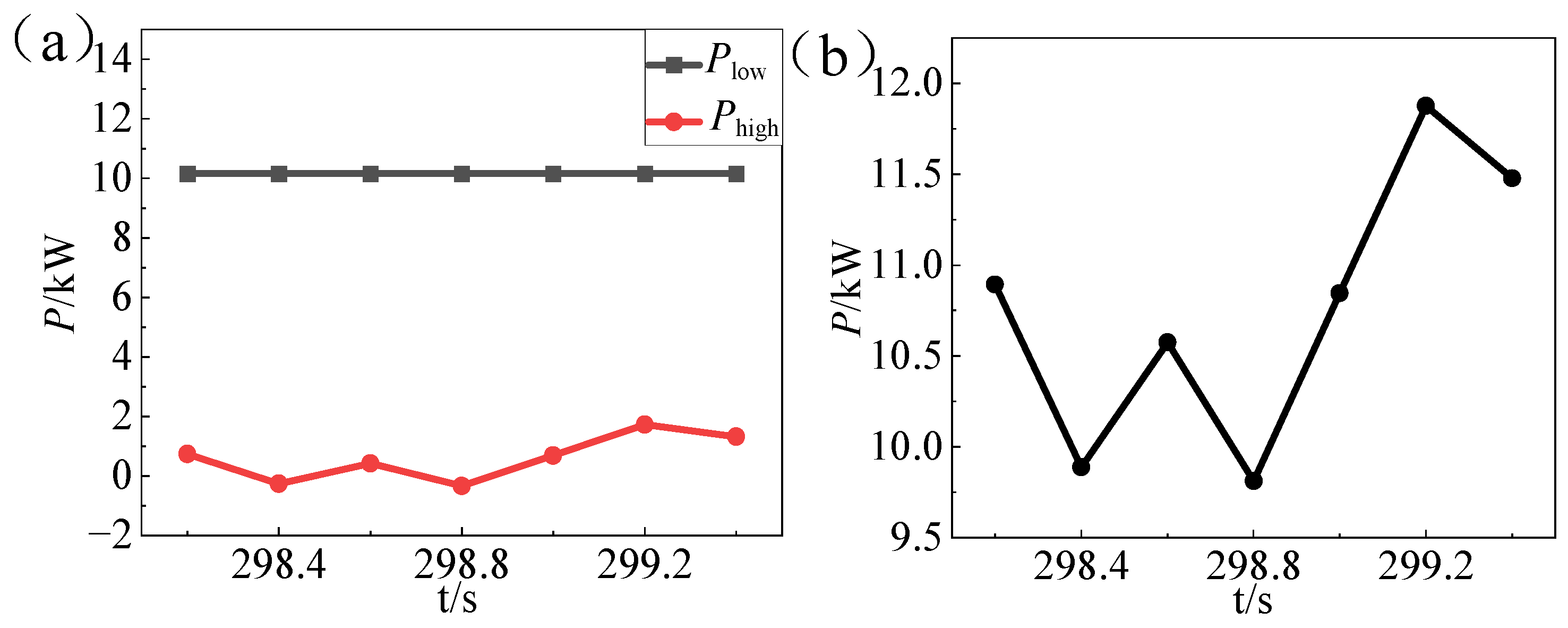
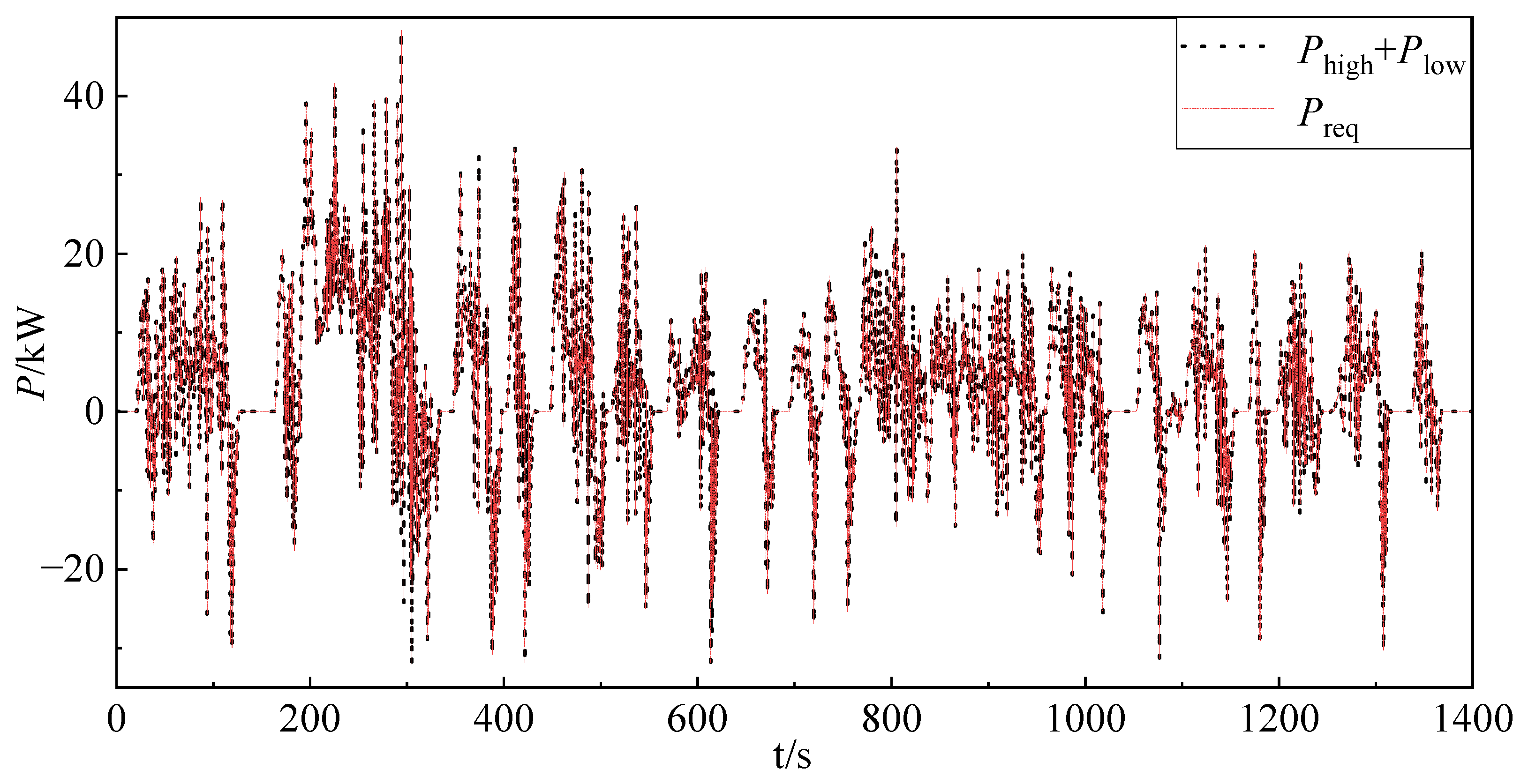
5.2.1. Haar Wavelet Simulation Verification

The ACC system predicts power demand for seven future timesteps by integrating real-time power demand and decomposing it into low-/high-frequency components through a third-order Haar wavelet transform. This process enables online rolling decomposition of the wavelet transform across successive prediction windows. As illustrated in Figure 14a, the low and high-frequency demand power following wavelet decomposition from 298.2 s to 299.4 s is depicted, while Figure 14b presents the demand power. The sum of wavelet-decomposed components must remain strictly consistent with the original demand power. As illustrated in Figure 14, the recorded original demand power values are 10.89 kW, 9.89 kW, 10.58 kW, 9.82 kW, 10.85 kW, 11.88 kW, and 11.48 kW. The decomposed high-frequency demand power components are 0.73 kW, −0.27 kW, 0.42 kW, −0.34 kW, 0.69 kW, 1.72 kW, and 1.32 kW, while the low-frequency demand power remains constant at 10.16 kW across all time points. Through mathematical verification, the algebraic sum at each timestamp demonstrates precise equivalence to the corresponding original demand power values. This analysis focuses exclusively on the demand power decomposition within a single prediction time domain. The trend of demand power decomposition for each prediction time domain during traveling is similar to Figure 14.

As demonstrated in Figure 15a–c, most of the high-frequency transient power is decomposed to P_high, with P_low consisting of all low-frequency steady-state power, in addition to a minor proportion of high-frequency transient power. As demonstrated in Figure 16, the summation derived from wavelet decomposition remains consistent with the demand power across all operational conditions. This further validates the strict adherence to energy conservation principles in wavelet-based decomposition methodologies. The absolute cumulative power values of P_high and P_low under driving and braking conditions are quantified as 13261 kW and 41680 kW, respectively. Notably, the magnitude of P_low exceeds P_high by a factor of 3.14. This pronounced disparity underscores the critical necessity for implementing secondary allocation strategies targeting P_low, thereby optimizing EMS frameworks to enhance systemic efficiency and sustainability.

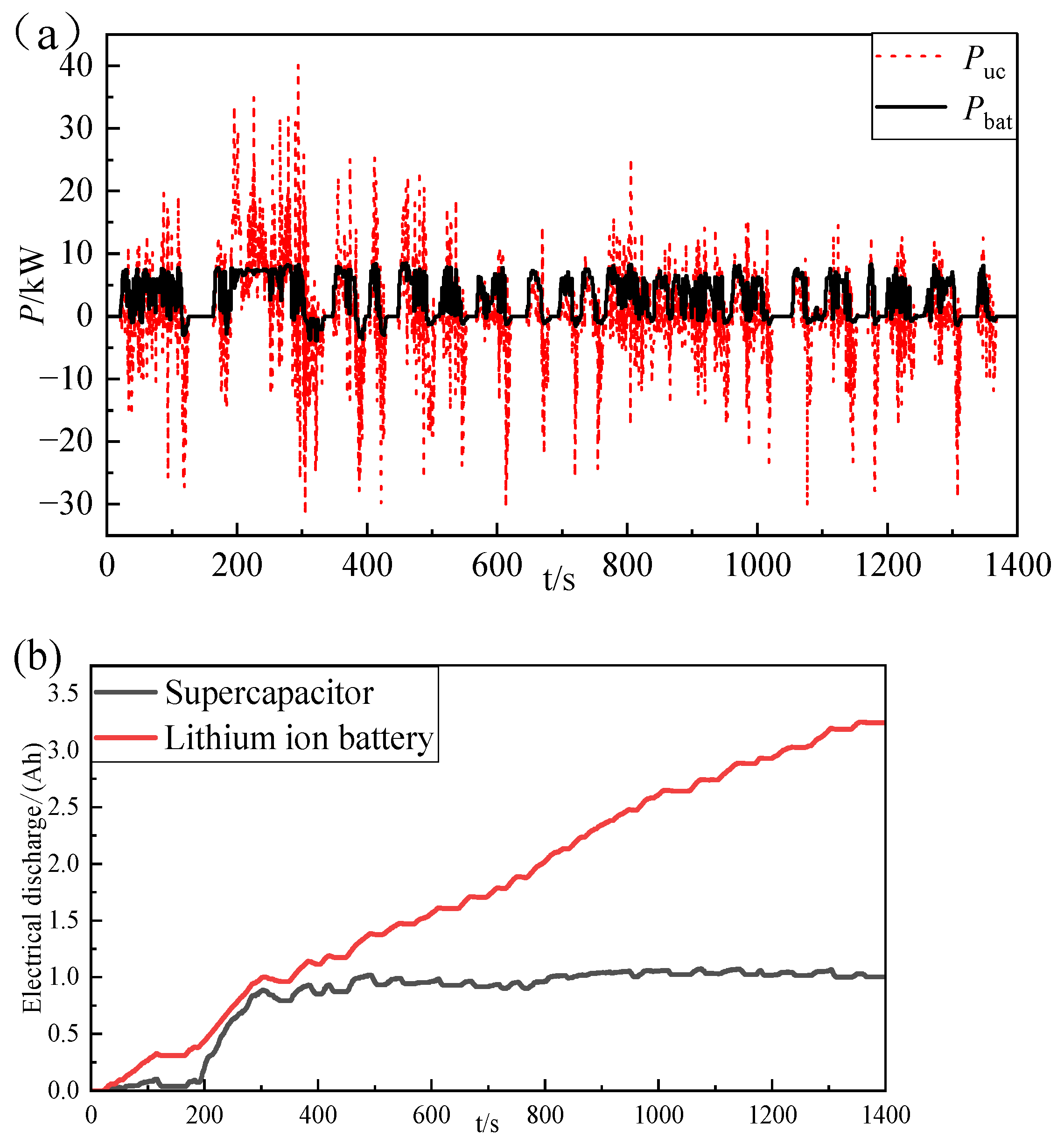
5.2.2. Fuzzy Logic Control Simulation Verification and Comparison

As demonstrated in Figure 17a and

Table 4. Mathematical statistics of HESS power distribution and charge-discharge under the wavelet-based fuzzy logic strategy.

Parameter	Pmax/kW	Pdrive,avg/kW	Pbrake,avg/kW	Q/Ah
Battery	8.53	4.66	−0.77	3.25
Supercapacitor	40.1	4.34	−4.37	1

, under driving conditions, the lithium-ion battery and supercapacitor are allocated to average power levels of 4.66 kW and 4.34 kW, respectively. The lithium-ion battery matches a large amount of low-frequency steady-state power demand, while the supercapacitor matches a large amount of high-frequency transient peak power. In the context of braking conditions, the average power of the lithium-ion battery and the supercapacitor is −0.77 kW and −4.37 kW, respectively. The lithium-ion battery exhibits a minor degree of energy recovery, while the supercapacitor demonstrates a greater capacity for energy retrieval. As shown in Figure 17b, the lithium-ion battery exhibits small variations in the slope of its charge-release curve, indicating stable discharge. Except for the 200–300 s period, the charge released by the supercapacitor during driving is nearly identical to the charge recovered during braking. Under the UDDS driving cycle, the front vehicle’s speed reaches its maximum within the 200–300 s interval. To ensure safe following distances at high speeds, the supercapacitor significantly increases its charge release to meet transient high-load demands while the lithium-ion battery maintains steady charge output. The lithium-ion battery exhibits a discharge capacity that is 3.25 times that of the supercapacitor, thereby indicating that lithium-ion batteries are the primary energy source.

The threshold logic filtering incorporates a low-pass filter into the logic threshold, thereby facilitating the smoothing of large currents that exceed the threshold. This approach is predominantly employed in scenarios involving high-frequency peak transient currents [45]. The following study will compare threshold logic filtering, wavelet-based logic thresholding, and wavelet-fuzzy logic, highlighting their respective advantages and disadvantages as illustrated in Figure 18 and

Table 5. Mathematical-statistical comparison of three energy management strategies.

Parameter	SOC/%	Ibat,max/A	Ibat,avg/A	Energy Consumption/J
Front vehicle	0.7231	167.06	18.9	1137275
Threshold logic filtering	0.74	55.71	11.01	1105196
Wavelet-based logic thresholding	0.7415	23.06	10.2	1077475
Wavelet-fuzzy logic	0.7459	26.49	9.37	1071748

. The thresholds for the threshold logic filtering and wavelet-based Logic thresholding are the positive and negative average values of the decomposed power, which are 8.24 kW, −5.59 kW, 7.46 kW, and −5.46 kW, respectively. Figure 18a compares current profiles at the maximum demand PowerPoint. The threshold logic filtering fails to smooth sub-threshold currents and exhibits limited capability in mitigating high-current surges, resulting in poor operational adaptability. The application of wavelet-based logic thresholding has been demonstrated to result in a smoother current flow, more stable current variations, and a substantial enhancement in the capacity to mitigate large currents. In comparison to wavelet-based logic thresholding, wavelet-fuzzy logic demonstrates a superior capacity to adapt to changing conditions. Furthermore, the average current is reduced throughout the range of driving conditions. As illustrated in Figure 18b, the initial SOC of the lithium-ion battery was set to 0.8 under three distinct control strategies. The final values of the threshold logic filtering, wavelet-based logic thresholding, and wavelet-fuzzy logic are 0.74, 0.7415, and 0.7459, respectively. The SOC is increased by 0.2% and 0.59%, respectively. Figure 18c demonstrates that the wavelet-fuzzy logic control achieves the lowest energy consumption, followed by the wavelet-based logic thresholding, while the threshold logic filtering exhibits the highest consumption, with energy reductions of 0.53% and 2.51%, respectively. Under the threshold logic filtering, the ego vehicle’s energy consumption is 2.82% lower than that of the front vehicle.

To statistically validate Figure 18 conclusions and exclude random fluctuation effects, the 1400-s operation was divided into seven 200 s intervals. Each interval was analyzed independently for average battery current I_bat,avg, state-of-charge (SOC) variations, and energy consumption, disregarding cumulative historical data. As illustrated in Figure 19a, the energy consumption can be categorized as follows: threshold logic filtering > wavelet-based logic thresholding > wavelet-fuzzy logic across all intervals. As illustrated in Figure 19b,c, the filter-logic threshold demonstrated poor operational adaptability, with larger SOC fluctuations and unstable I_bat,avg. Both wavelet-based strategies exhibited superior robustness, particularly the wavelet-fuzzy logic, which maintained smoother current discharge profiles alongside systematically reduced I_bat,avg and SOC variations compared to wavelet-based logic thresholding.

6. Conclusions

This study develops an online EMS for HESEV in car-following scenarios, optimizing lithium-ion battery usage by reducing high-frequency transient power allocation while improving energy efficiency. Firstly, a car-following dynamics model and a HESS model were established separately. Subsequently, a multi-objective function considering both optimal tracking quality and energy economy was formulated, which was optimized and solved using the NSGA-II algorithm. Following this, under car-following operating conditions, the demand power was decomposed through online rolling decomposition based on third-order Haar wavelet theory, while the low-frequency steady-state demand power underwent secondary decomposition via a fuzzy logic control strategy. Finally, the following conclusions are drawn through simulation analysis.

(1)

After multi-objective optimization using NSGA-II for optimal tracking quality and energy economy, the maximum relative speed between vehicles is 2.7 m/s with an average relative speed of 0.56 m/s. The relative distance remains within the desired range, accompanied by a 3.71% reduction in total power demand. The ego vehicle demonstrates stable following capability with improved energy economy. The SOC of the lithium-ion battery in the dual-source system decreases more gradually compared to single-source configurations.

(2)

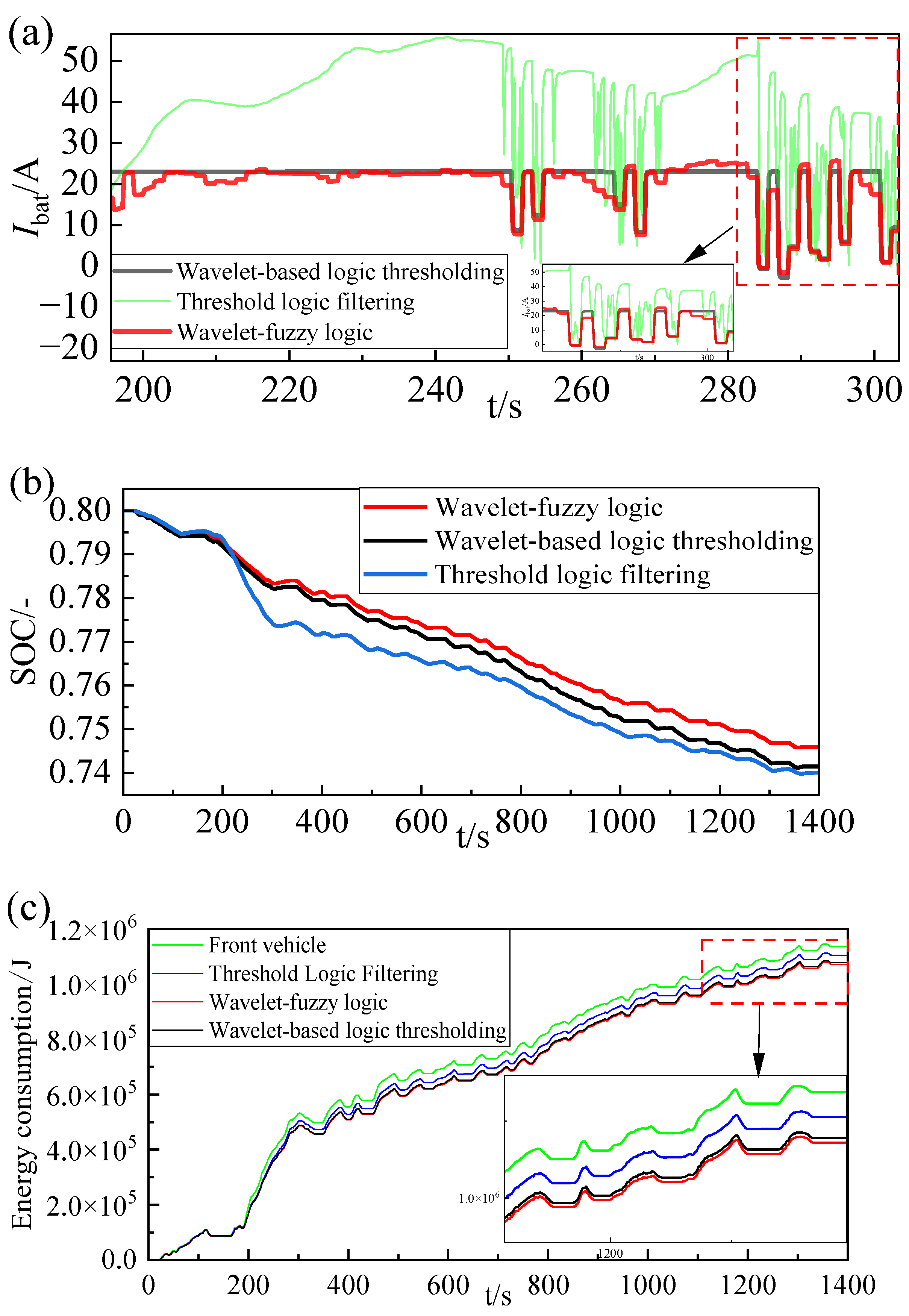
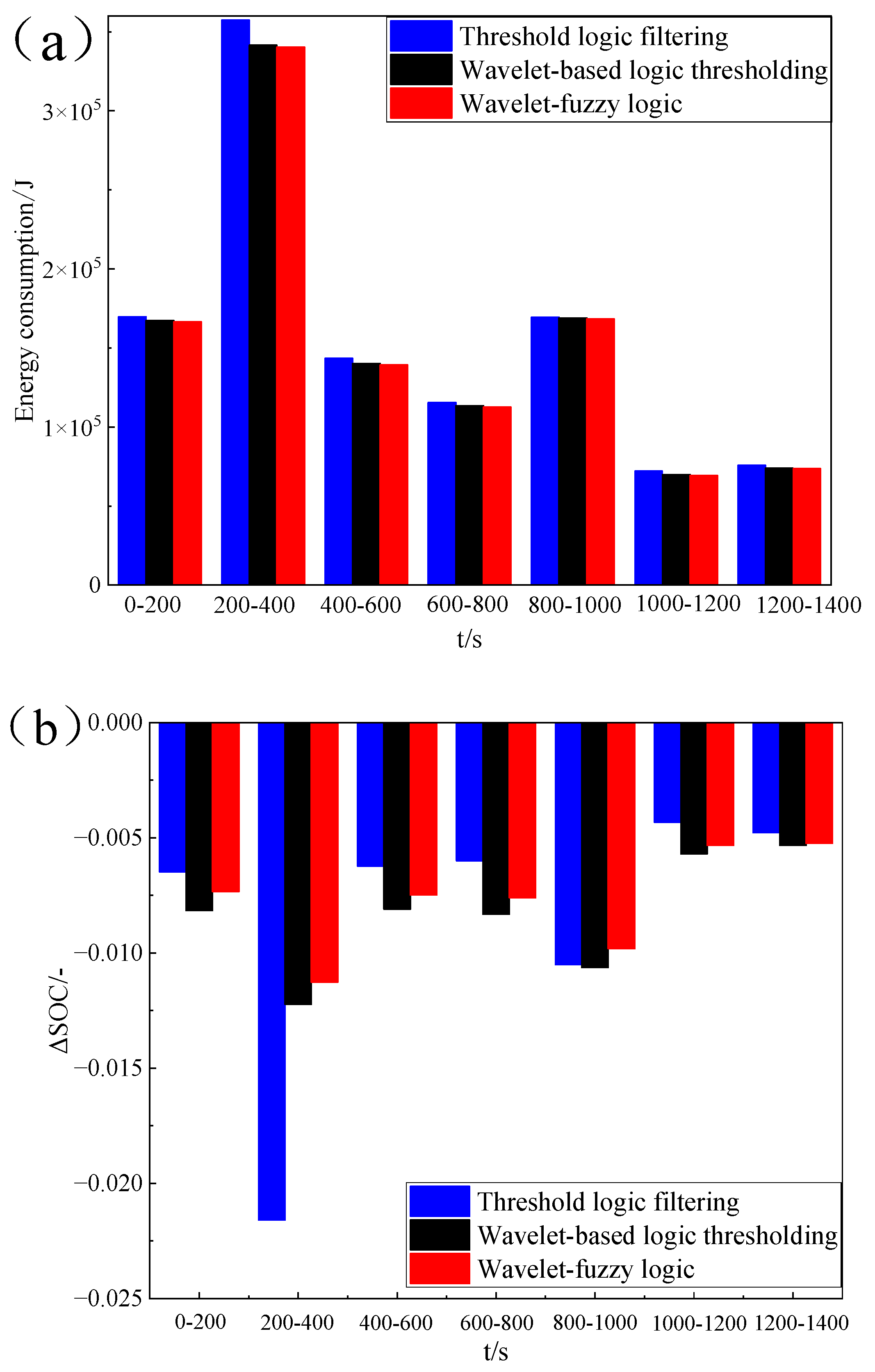
The high-frequency transient power of lithium-ion batteries is significantly reduced after online rolling decomposition based on third-order Haar theory. The wavelet-based logic thresholding is demonstrably superior in terms of control when compared with threshold logic filtering. This is evidenced by a more uniform current, a substantial decrease in peak current, and a 2.51% reduction in energy consumption.

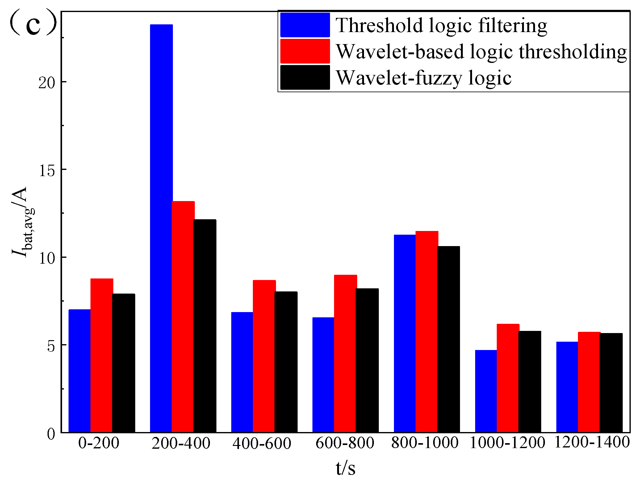
(3)

Compared to the wavelet-based logic threshold, the wavelet-fuzzy logic approach demonstrates superior adaptability to operational condition variations and lower energy consumption. These improvements are validated by an 8.1% reduction in average battery current and a 0.59% increase in SOC of the lithium-ion battery.

The ACC-WT hierarchical control framework reduces high-frequency transient power allocation to lithium-ion batteries and lowers energy consumption in HESS. However, its dependency on finite-horizon power demand prediction introduces feedback delays, compromising vehicle tracking performance. Additionally, the framework’s nonlinear adaptability remains unverified. Future work will optimize the prediction horizon-wavelet decomposition correlation under nonlinear conditions and explore tracking accuracy, energy efficiency, and battery lifespan trade-offs. This will advance online EMS for HESEV under ACC scenarios.

References

- Peng, J.; Fan, Y.; Yin, G.; Jiang, R. Collaborative Optimization of Energy Management Strategy and Adaptive Cruise Control Based on Deep Reinforcement Learning. IEEE Trans. Transp. Electrif. 2022, 9, 34–44. [Google Scholar]
- Li, J.; Chen, C.; Yang, B.; He, J.; Guan, X. Energy-Efficient Cooperative Adaptive Cruise Control for Electric Vehicle Platooning. IEEE Trans. Intell. Transp. Syst. 2023, 25, 4862–4875. [Google Scholar]
- Zhu, L.; Tao, F.; Fu, Z.; Wang, N.; Ji, B.; Dong, Y. Optimization Based Adaptive Cruise Control and Energy Management Strategy for Connected and Automated FCHEV. IEEE Trans. Intell. Transp. Syst. 2022, 23, 21620–21629. [Google Scholar]
- Kural, E.; Güvenç, B.A. Integrated Adaptive Cruise Control for Parallel Hybrid Vehicle Energy Management. IFAC-PapersOnLine 2015, 48, 313–319. [Google Scholar]
- He, Y.; Zhou, Q.; Makridis, M.; Mattas, K.; Li, J.; Williams, H.; Xu, H. Multiobjective Co-Optimization of Cooperative Adaptive Cruise Control and Energy Management Strategy for PHEVs. IEEE Trans. Transp. Electrif. 2020, 6, 346–355. [Google Scholar]
- Li, S.; Chu, L.; Fu, P.; Pu, S.; Wang, Y.; Li, J.; Guo, Z. Energy-Oriented Hybrid Cooperative Adaptive Cruise Control for Fuel Cell Electric Vehicle Platoons. Sensors 2024, 24, 5065. [Google Scholar] [CrossRef]
- Aljohani, T.M.; Ebrahim, A.; Mohammed, O. Real-Time Metadata-Driven Routing Optimization for Electric Vehicle Energy Consumption Minimization Using Deep Reinforcement Learning and Markov Chain Model. Electr. Power Syst. Res. 2021, 192, 106962. [Google Scholar]
- Aslan Yıldız, Ö.; Sarıçiçek, İ.; Yazıcı, A. A Reinforcement Learning-Based Solution for the Capacitated Electric Vehicle Routing Problem from the Last-Mile Delivery Perspective. Appl. Sci. 2025, 15, 1068. [Google Scholar] [CrossRef]
- Lu, C.; Dong, J.; Hu, L. Energy-Efficient Adaptive Cruise Control for Electric Connected and Autonomous Vehicles. IEEE Intell. Transp. Syst. Mag. 2019, 11, 42–55. [Google Scholar]
- Li, G.; Görges, D. Ecological Adaptive Cruise Control and Energy Management Strategy for Hybrid Electric Vehicles Based on Heuristic Dynamic Programming. IEEE Trans. Intell. Transp. Syst. 2018, 20, 3526–3535. [Google Scholar]
- Zhang, R.; Wu, N.; Wang, Z.; Li, K.; Song, Z.; Chang, Z.; Chen, X.; Yu, F. Constrained Hybrid Optimal Model Predictive Control for Intelligent Electric Vehicle Adaptive Cruise Using Energy Storage Management Strategy. J. Energy Storage 2023, 65, 107383. [Google Scholar]
- Yu, S.; Pan, X.; Georgiou, A.; Chen, B.; Jaimoukha, I.M.; Evangelou, S.A. A Real-Time Robust Ecological-Adaptive Cruise Control Strategy for Battery Electric Vehicles. IEEE Trans. Transp. Electrif. 2023, 10, 7389–7404. [Google Scholar]
- Wang, C.; Xiong, R.; He, H.; Zhang, Y.; Shen, W. Comparison of Decomposition Levels for Wavelet Transform Based Energy Management in a Plug-in Hybrid Electric Vehicle. J. Clean. Prod. 2019, 210, 1085–1097. [Google Scholar]
- Ibrahim, M.; Jemei, S.; Wimmer, G.; Hissel, D. Nonlinear Autoregressive Neural Network in an Energy Management Strategy for Battery/Ultra-Capacitor Hybrid Electrical Vehicles. Electr. Power Syst. Res. 2016, 136, 262–269. [Google Scholar]
- Yan, M.; Li, M.; He, H.; Peng, J.; Sun, C. Rule-Based Energy Management for Dual-Source Electric Buses Extracted by Wavelet Transform. J. Clean. Prod. 2018, 189, 116–127. [Google Scholar]
- Zhang, Z.; Tang, J.; Zhang, J.; Zhang, T. Research on Energy Hierarchical Management and Optimal Control of Compound Power Electric Vehicle. Energies 2024, 17, 1359. [Google Scholar] [CrossRef]
- Zhang, Z.; Du, W.; Liang, J.; Zhang, Y.; Wu, Y. Layered Control of Compound Power Loader Based on Fuel Cell. J. Beijing Univ. Aeronaut. Astronaut. 2022, 48, 2165–2176. [Google Scholar]
- Liu, Y. Research on Energy-saving Adaptive Cruise Control for Pure electric Vehicles. Master’s Thesis, Chongqing University, Chongqing, China, 2021. [Google Scholar]
- Huan, J.; Wei, W.; Zou, D. Research on Mode Switching Strategy of Adaptive Cruise System based on Personalized Spacing Strategy. Automot. Eng. 2020, 42, 1302–1311. [Google Scholar]
- Li, S.; Li, K.; Rajamani, R.; Wang, J. Model Predictive Multi-objective Vehicular Adaptive Cruise Control. IEEE Trans. Control Syst. Technol. 2010, 19, 556–566. [Google Scholar]
- Santhanakrishnan, K.; Rajamani, R. On Spacing Policies for Highway Vehicle Automation. IEEE Trans. Intell. Transp. Syst. 2003, 4, 198–204. [Google Scholar]
- Rajamani, R. Vehicle Dynamics and Control; Springer: Berlin/Heidelberg, Germany, 2011. [Google Scholar]
- Zhang, Q.; Hou, J.; Hu, X.; Yuan, L.; Jankowski, Ł.; An, X.; Duan, Z. Vehicle Parameter Identification and Road Roughness Estimation Using Vehicle Responses Measured in Field Tests. Measurement 2022, 199, 111348. [Google Scholar] [CrossRef]
- Lv, Y.-M.; Yuan, H.-W.; Liu, Y.-Y.; Wang, Q.-S. Fuzzy Logic based Energy Management Strategy of Battery-ultracapacitor single power supply for HEV. In Proceedings of the 2010 First International Conference on Pervasive Computing, Signal Processing and Applications, Harbin, China, 17–19 September 2010; pp. 1209–1214. [Google Scholar]
- Hemmati, R.; Saboori, H. Emergence of Hybrid Energy Storage Systems in Renewable Energy and Transport Applications–A Review. Renew. Sustain. Energy Rev. 2016, 65, 11–23. [Google Scholar] [CrossRef]
- Yuan, Z.; Tian, T.; Hao, F. A Hybrid Neural Network Based on Variational Mode Decomposition Denoising for Predicting State-of-Health of Lithium-Ion Batteries. J. Power Sources 2024, 609, 234697. [Google Scholar] [CrossRef]
- Li, Y.; Wu, Y.; Huang, H. Neural Network-Based Modeling of Diffusion-Induced Stress in a Hollow Cylindrical Nano-Electrode of Lithium-Ion Battery. J. Electrochem. Energy Convers. Storage 2025, 22, 011011. [Google Scholar] [CrossRef]
- Hoque, M.A.; Hassan, M.K.; Hajjo, A.; Tokhi, M.O. Neural Network-Based Li-Ion Battery Aging Model at Accelerated C-Rate. Batteries 2023, 9, 93. [Google Scholar] [CrossRef]
- Sarkar, S.; Halim, S.Z.; El-Halwagi, M.M. Electrochemical Models: Methods and Applications for Safer Lithium-Ion Battery Operation. J. Electrochem. Soc. 2022, 169, 100501. [Google Scholar] [CrossRef]
- Bhat, C.; Channegowda, J. An Improved Electrochemical-Based Model to Estimate Battery Equivalent Circuit Parameters for Pulsed Discharge Scenarios. Energy Storage 2022, 4, e294. [Google Scholar] [CrossRef]
- Lagnoni, M.; Scarpelli, C.; Lutzemberger, G. Critical Comparison of Equivalent Circuit and Physics-Based Models for Lithium-Ion Batteries: A Graphite/Lithium-Iron-Phosphate Case Study. J. Energy Storage 2024, 94, 112326. [Google Scholar] [CrossRef]
- Cheng, Y.S. Identification of Parameters for Equivalent Circuit Model of Li-Ion Battery Cell with Population Based Optimization Algorithms. Ain Shams Eng. J. 2024, 15, 102481. [Google Scholar] [CrossRef]
- Graule, A.; Oehler, F.F.; Schmitt, J. Development and Evaluation of a Physicochemical Equivalent Circuit Model for Lithium-Ion Batteries. J. Electrochem. Soc. 2024, 171, 020503. [Google Scholar] [CrossRef]
- Hussein, H.M.; Esoofally, M.; Donekal, A.; Rafin, S.M.S.H.; Mohammed, O. Comparative Study-Based Data-Driven Models for Lithium-Ion Battery State-of-Charge Estimation. Batteries 2024, 10, 89. [Google Scholar] [CrossRef]
- Mu, G.; Wei, Q.; Xu, Y. State of Health Estimation of Lithium-Ion Batteries Based on Feature Optimization and Data-Driven Models. Energy 2025, 314, 134578. [Google Scholar] [CrossRef]
- Zheng, X.; Wu, F.; Tao, L. Degradation Trajectory Prediction of Lithium-Ion Batteries Based on Charging-Discharging Health Features Extraction and Integrated Data-Driven Models. Qual. Reliab. Eng. Int. 2024, 40, 1833–1854. [Google Scholar] [CrossRef]
- Zhang, W.; Xie, Y.; He, H. Multi-Physics Coupling Model Parameter Identification of Lithium-Ion Battery Based on Data Driven Method and Genetic Algorithm. Energy 2025, 314, 134120. [Google Scholar] [CrossRef]
- Shi, J. Research on Adaptive Cruise Control Algorithm considering Road Conditions. Master’s Thesis, Jilin University, Changchun, China, 2019. [Google Scholar]
- Aljohani, T.M.; Mohammed, O. A Real-Time Energy Consumption Minimization Framework for Electric Vehicles Routing Optimization Based on SARSA Reinforcement Learning. Vehicles 2022, 4, 1176–1194. [Google Scholar] [CrossRef]
- Luo, Y.; Chen, T.; Zhang, S.; Li, K. Intelligent Hybrid Electric Vehicle ACC with Coordinated Control of Tracking Ability, Fuel Economy, and Ride Comfort. IEEE Trans. Intell. Transp. Syst. 2015, 16, 2303–2308. [Google Scholar] [CrossRef]
- Pan, C.; Huang, A.; Wang, J.; Chen, L.; Liang, J.; Zhou, W.; Wang, L.; Yang, J. Energy-optimal Adaptive Cruise Control Strategy for Electric Vehicles based on Model Predictive Control. Energy 2022, 241, 122793. [Google Scholar]
- Yan, W. Research on Improved Genetic Algorithm Based on Multi-objective optimization Problem. Master’s Thesis, Tianjin Polytechnic University, Tianjin, China, 2019. [Google Scholar]
- Zhang, X.; Mi, C. Vehicle Energy Management: Modeling, Control and Optimization; Zhang, X.; Mi, C., Translators; China Machine Press: Beijing, China, 2013; pp. 113–140. [Google Scholar]
- Kakouche, K.; Oubelaid, A.; Mezani, S.; Rekioua, D.; Rekioua, T. Different Control Techniques of Permanent Magnet Synchronous Motor with Fuzzy Logic for Electric Vehicles: Analysis, Modelling, and Comparison. Energies 2023, 16, 3116. [Google Scholar] [CrossRef]
- Wang, B. Research on Parameter Matching and Control Strategy of New Energy Vehicle Power System. Master’s Thesis, Hunan University, Changsha, China, 2018. [Google Scholar]