A New Endogenous Direction Selection Mechanism for the Direction Distance Function Method Applied to Different Economic–Environmental Development Modes

Abstract

As a direction selection in the direction distance function (DDF), endogenous DDF can accurately reflect the numerical characteristics of inputs/outputs, but it is difficult to effectively popularize. And it is also difficult to effectively combine with reality. To solve those problems, this paper introduces slack variables to construct a new endogenous direction-setting mechanism, which makes the endogenous model have the conditions to be popularized. Based on the original endogenous DDF, we consider environmental concern, economic concern, coordinated development, and priority development, and then construct six new extended DDF models with slack variables. Based on priority development, we further propose six new extended DDF models. These new extended models can not only realize the complete internalization of direction determination but also overcome the limitations of traditional endogenous models. Combined with the actual case, the emission reduction potential of different areas is revealed, and the improved path is proposed. The results show that the new extended DDF models effectively reflect the different development modes of carbon emissions, and different development modes have a significant impact on emission reduction potential. In addition, compared with economic concern and priority development, coordinated development and environmental concern are most beneficial to carbon emission reduction, but the development mode of environmental concern can better reveal the improved path of environmental development.

1. Introduction

Global warming has effects on the natural economic environment and human health, which have drawn more attention all over the world [1]. The International Energy Agency (IEA) released the report “CO₂ Emissions in 2022”, which showed that the global energy-related CO₂ emissions are relatively high in 2022, reaching more than 36.8 billion tons, 0.9% over the previous year. The growth rate of CO₂ in 2022 is much lower than the global GDP growth rate of 3.2%, which continues the trend of decoupling CO₂ emissions from economic growth in the past decade. Therefore, the study of environmental efficiency has great significance to sustainable development. The evaluation of environmental efficiency and production of pollutants can be traced back to Pittman [2], who first considered pollutants to be an undesirable output. Most previous studies exploring environmental efficiency are based on distance functions [3], and in recent years, the directional distance function has attracted much attention.

The directional distance function (DDF), which originated from the distance function and the gauge function, is an extension of data envelopment analysis (DEA), and it is suitable for similar decision-making units (DMU) with multiple inputs/outputs. The DDF method can estimate the efficiency level in any direction for DMUs, which is the advantage of this method. The DDF method breaks the limitation of traditional DEA radial measurement, is recognized by DEA researchers, and has become a nonparametric research method widely used in economics and management [4]. Subsequently, Chung and Färe [5] and Chambers et al. [6] discussed the basic situation, including undesirable output, which made great contributions to the theoretical development of the DDF method, and thus, its research field has gradually expanded to environmental efficiency evaluation. Now it has become one of the important tools to measure carbon emission efficiency. This mainly includes a carbon emission efficiency assessment [7,8,9], emission reduction potential [10], and emission reduction cost assessment [11]. The research on the DDF has been emerging in recent years. However, in most related studies, the flexibility of direction selection in DDF is flawed, and the rationality analysis of direction selection is easily ignored. Ma et al. [12] found that a small change in the direction vector may lead to a big bias in the results. Therefore, reasonable direction selection is important, and it is the basis for the DDF method to measure the relative efficiency of DMUs. But, none of the above research involves the choice of direction.

At present, the research on DDF is mainly divided into three categories. First is the traditional exogenous direction selection method, which usually depends on the subjective setting of the direction vector by researcher [13]. Although it is simple and easy to operate, it lacks adaptability to data characteristics, which may lead to a disconnect between the model results and the actual external environment. Second is the endogenous direction selection method, which determines the direction based on the spatial relationship between DMU and the frontier. It can reflect the numerical characteristics of input/output and then improve the accuracy and applicability of the model. However, in practical applications, it still faces challenges, such as difficulties in popularization and insufficient combination with real-world scenarios. Third is the direction selection method combined with the external environment, that is, considering the external environment (such as profit, policy) and numerical characteristics of the DMU to determine direction. By combining subjective and objective elements, this method provides sufficient theoretical support for direction selection. For example, Chambers et al. [6] introduced DDF and established the corresponding relationship between DDF and profit function. Subsequently, many scholars considered the profit function when using DDF [14,15,16]. Therefore, based on the third and second categories, this paper provides a new idea for the study on coordinated development of the economy and the environment.

Although endogenous direction can overcome the defects of exogenous direction, and thus evaluate carbon emissions more effectively, the endogenous DDF method still has obvious limitations in practical applications. On the one hand, endogenous direction is easily limited to simple numerical relations, and the nonlinear framework is difficult to popularize, which leads to the fact that most of the carbon emission assessment research is still dominated by the exogenous DDF method [17,18]. On the other hand, although endogenous DDF possesses significant theoretical advantages, it still faces two major challenges regarding practical applications. First, the promotion is insufficient, and it is difficult to adapt to a varied economic environment. Second, the combination with practical problems is not close enough, which limits its policy-guiding significance.

This paper mainly solves the above limitations from the following aspects. First, in the aspect that endogenous DDF is difficult to extend effectively, this paper contributes to the literature by introducing slack variables to construct a new endogenous direction-setting mechanism, which makes the endogenous model have the conditions to be popularized. Meanwhile, it can also promote the development of endogenous DDF in the field of environmental efficiency evaluation. Second, in the way it combines endogenous DDF with environmental problems, this paper contributes to the literature by measuring the potential of carbon emission reduction under various development modes, including economic concern, environmental concern, coordinated development, and priority development, and then constructs twelve new extended DDF models. Moreover, this combination method avoids the influence of arbitrary mapping rules and captures the nature of different environmental development modes. To the best of our knowledge, this is the first study that uses an endogenously determined directional vector to explore the impact of different development modes on emission reduction potential. Finally, in the aspect of the improvement path in carbon emission levels, this paper analyzes the carbon emission data of fifteen years, which can provide a reliable practical reference for effectively stimulating the potential of carbon emission reduction.

The remainder of this paper is organized as follows. Section 2 reviews the DDF method and the weak disposability hypothesis. Section 3 proposes different development models and constructs twelve new DDF extended models. In Section 4, the case is evaluated by using the carbon emission data of fifteen years, and the emission potential under different development modes is compared. The improvement path is provided, and the conclusions are then given in Section 5.

2. Preliminaries

2.1. Weak Disposability

According to Färe et al. [19], the weak disposability hypothesis is defined as follows:

$$P^w\left(X\right)=\left\{\left(Y,Z\right)\left|{\displaystyle \sum _{j=1}^n{\lambda }_j{Y}_j\ge Y,{\displaystyle \sum _{j=1}^n{\lambda }_j{Z}_j=Z,{\displaystyle \sum _{j=1}^n{\lambda }_j{X}_j\le X,{\lambda }_j\ge 0\left(j=1,2,\cdots ,n\right)}}}\right.\right\}$$

(1)

where ${\lambda }_j$ is the intensive variable. The inequality constraints on input $x$ and desirable output $y$ indicate that both of them are under strong disposability, and thus, decision makers are free to increase or decrease them according to their own needs. Meanwhile, the equation of undesirable outputs $z$ means that undesirable outputs have weak disposability. That is, decision makers cannot reduce them without affecting the inputs and the desirable outputs. To combine with reality, the undesirable outputs in this paper are treated with weak disposability.

2.2. Exogenous DDF

Suppose that there are $n$ DMUs to be evaluated, and for each DMU_d, $x_d=(x_{1d},x_{2d},\dots ,x_{md})\in R_{+}^m$ is the input vector, $y_d=(y_{1d},y_{2d},\dots ,y_{sd})\in R_{+}^s$ is the desirable output vector, and $z_d=(z_{1d},z_{2d},\dots ,z_{hd})\in R_{+}^h$ is the undesirable output vector. Assuming that input $x$ can produce desirable output $y$ and undesirable output $z$, then the production possibility set can be expressed as $P(x)=\left\{(x,y,z)\left|x can produce(y,z)\right.\right\}$. According to the research of Kaneko et al. [20], ${\overrightarrow{D}}_k=(x,y,z;g_y,-g_z)$ can be solved by the linear programming method, and the direction distance function is abbreviated as $\beta$. Then, for any DMU_d, the exogenous DDF model can be constructed as follows.

$$\begin{array}{l}Max\beta \\ s.t. {\displaystyle \sum _{j=1}^n{\lambda }_j{x}_{ij}\le x_{id}, i=1,\dots ,m; }\\ \hspace{1em} {\displaystyle \sum _{j=1}^n{\lambda }_j{y}_{rj}\ge y_{rd}+{\beta }_d{g}_y, r=1,\dots ,s;}\\ \hspace{1em} {\displaystyle \sum _{j=1}^n{\lambda }_j{z}_{fj}=z_{fd}-{\beta }_d{g}_z, f=1,\dots ,h};\\ \hspace{1em} \forall {\lambda }_j\ge 0,{\beta }_d \mathrm{unconstrained}. \end{array}$$

(2)

Among them, $\lambda$ gives each DMU different weights. At present, the related research mainly defines the direction vector $g=(g_y,-g_z)$ as three different directions: $(y,z)$, $(y,0)$, and $(0,z)$.

2.3. Endogenous DDF

The evaluation of the exogenous DDF model depends on the choice of direction vector by researchers, which makes the results have a highly subjective component. To overcome this defect, an endogenous direction distance function model is proposed by Färe et al. [21]. That is, the optimal direction vector is solved endogenously through the model. This model is applied to environmental efficiency measurement by Hampf and Krüger [22], which scales all outputs in weighted proportions, and the endogenous DDF model is expressed as follows:

$$\begin{array}{l}Max{\beta }_d\\ s.t. {\displaystyle \sum _{j=1}^n{\lambda }_j{x}_{ij}\le x_{id}, i=1,\dots ,m; }\\ \hspace{1em} {\displaystyle \sum _{j=1}^n{\lambda }_j{y}_{rj}\ge y_{rd}+{\beta }_d{\alpha }_d\odot y_{rd}, r=1,\dots ,s;}\\ \hspace{1em} {\displaystyle \sum _{j=1}^n{\lambda }_j{z}_{fj}=z_{fd}-{\beta }_d{\delta }_d\odot z_{fd}, f=1,\dots ,h};\\ \hspace{1em} {\displaystyle \sum _{d=1}^n{\alpha }_d+{\delta }_d=1, d=1,\dots ,n;}\\ \hspace{1em} \forall {\lambda }_j,{\alpha }_d,{\delta }_d\ge 0, {\beta }_d \mathrm{unconstrained}. \end{array}$$

(3)

Model (3) is nonlinear, and it can be linearized by introducing the new variables $\gamma =1/\beta$ and $\mu =\lambda /\beta$. Vector ${\alpha }_d$ represents the weight of desirable output increase, and vector ${\delta }_d$ represents the weight of undesirable output decrease. ${\alpha }_d$ and ${\delta }_d$ are non-negativity, which indicate that the desirable output can only increase and the undesirable output can only decrease. The operation symbol ⊙ stands for Hadamard product operation. ${\beta }_d^{\ast }\left(x_d,y_d,z_d\right)$ is the resulting efficiency measure of Model (3). Model (3) is more suitable for the measurement and expansion of environmental efficiency. Therefore, this paper extends the following models based on it and linearizes the extended DDF models by introducing $\gamma$ and $\mu$ to solve it.

3. Methodology

As shown in Figure 1, at present, the related research mainly defines the direction vector $g=(g_y,g_z)$ as three different directions: $(y,z)$, $(y,0)$, and $(0,z)$. That is, to make the desirable output and the undesirable output approach the frontier at 45 degrees, increase only the desirable output and decrease only the undesirable output. Moreover, these three directions are indicated by A₁, A₂, and A₃ in Figure 1, respectively. However, this given direction vector has a defect. That is, the evaluation of efficiency depends on the choice of direction vector by researchers, which makes the results have a high subjective component.

Therefore, this paper introduces slack variables as a tool to determine the endogenous direction. As shown in Figure 2, both A and B are ineffective DMUs, and they can freely determine the improvement direction, as shown in A₁ and B₁. Among them, A₂ and A₃ are two extreme direction choices of A. However, these two points are not in the production possibility set but only represent the interval of direction selection based on the slack variables. By restricting the slack variables, the selection of endogenous direction vectors can be influenced, and A₁₂ is the direction selection after minimizing S⁻. Meanwhile, A₁₃ is the direction selection after minimizing S⁺. Obviously, the selection of endogenous direction avoids the influence of decision makers and is more flexible.

Compared with Figure 1, by introducing slack variables into the endogenous direction selection mechanism, the direction vector can be dynamically adjusted based on different sustainable development goals, thus more accurately capturing the improvement potential of inefficient DMUs. The model with a direction set in Figure 2 can better reflect the problems of resource waste and environmental inefficiency in the actual production process, thus providing a more scientific basis for policy formulation.

By Figure 1 and Figure 2, compared with the exogenous direction, the advantages of the endogenous direction are as follows. (1) For accuracy improvement, the exogenous direction cannot accurately reflect the complexity of sustainable development. According to different goal setting, the endogenous direction can evaluate efficiency more flexibly based on the trade-off relationship between economic growth and environmental protection. (2) For enhanced policy relevance, the endogenous direction selection method can dynamically adjust the direction vector according to different sustainable development goals (such as maximizing economic growth and minimizing carbon emissions), thus providing more targeted decision support for policy makers. (3) For applicability expansion, the endogenous direction selection mechanism can better balance the relationship between economic growth and environmental protection and then support the realization of the SDGs.

3.1. Economic Concern Model (ECM₁)

Definition 1. 

Economic concern mode, a development mode with economic growth as its core goal, emphasizes increasing inputs to obtain more desirable outputs to promote economic development.

Economic development has a significant impact on carbon emissions, and Chien et al. [23] have proven that economic development can significantly reduce carbon emissions. This finding is closely related to Sustainable Development Goals (SDGs) 8 (Decent Work and Economic Growth) and 13 (Climate Action). Globally, many countries have promised to achieve carbon neutrality through green economic development. Therefore, realizing emission reduction targets within the framework of economic growth has become a crucial issue in sustainable development. In this section, the slack variables are used to expand the endogenous DDF Model (3). On this basis, the economic concern DDF model is constructed as follows.

$$\begin{array}{l}Min s_r^{+}\\ s.t. {\displaystyle \sum _{j=1}^n{\lambda }_j{x}_{ij}=x_{id}-s_i^{-}, i=1,\dots ,m; }\\ \hspace{1em} {\displaystyle \sum _{j=1}^n{\lambda }_j{y}_{rj}=y_{rd}+{\beta }_d{\alpha }_d\odot y_{rd}+s_r^{+}, r=1,\dots ,s;}\\ \hspace{1em} {\displaystyle \sum _{j=1}^n{\lambda }_j{z}_{fj}=z_{fd}-{\beta }_d{\delta }_d\odot z_{fd}, f=1,\dots ,h};\\ \hspace{1em} {\displaystyle \sum _{d=1}^n{\alpha }_d+{\delta }_d=1, d=1,\dots ,n;}\\ \hspace{1em} \forall {\lambda }_j,s_i^{-},s_r^{+},{\alpha }_d,{\delta }_d\ge 0, {\beta }_d \mathrm{unconstrained}. \end{array}$$

(4)

Model (4) is nonlinear, and it can be linearized by introducing the new variables $\gamma =1/\beta$ and $\mu =\lambda /\beta$. Moreover, the following extended DDF models can all be linearized in this way. Among them, the subscript $d$ represents the DMU being evaluated. ${\lambda }_j,{\beta }_d,s_i^{-},s_r^{+}$ are all decision variables. Vector ${\alpha }_d$ represents the weight of the desirable output increase, and vector ${\delta }_d$ represents the weight of undesirable output decrease, ${\alpha }_d$ and ${\delta }_d$ are non-negativity, which indicate that the desirable output can only increase, and the undesirable output can only decrease. Constraint 3 represents the weak disposability of the undesirable output.

Economic concern mode, with GDP growth as the core, is increasing investment to obtain a more ideal output. The slack variable represents the degree of improvement in the output. In the economic concern model, the smaller the slack variable $s_r^{+}$, the shorter the DMU improvement path for desirable output. By minimizing $s_r^{+}$, the objective function minimizes the optimal improvement path of the desirable output and then maximizes the relative efficiency of the desirable output. Thus, Model (4) can obtain the optimal endogenous direction under economic concern.

Theorem 1. 

The optimal solution of Model (4) reflects the situation of priority environmental development.

Proof. 

If there is ${\displaystyle \sum _{j=1}^n{\lambda }_j{x}_{ij}\le x_{id}}$, ${\displaystyle \sum _{j=1}^n{\lambda }_j{y}_{rj}\ge y_{rd}+{\beta }_d{\alpha }_d{y}_{rd}}$ and both inequalities have extreme conditions that make them equal. $s_r^{+}$ and $s_i^{-}$ can be used to bridge the gap between inequalities. Because $\forall s_r^{+}\ge 0$ is constant, and then the objective function is set to the minimum value of $s_r^{+}$, thus, the solution obtained is within the range of the above production possible set, and there is a feasible solution satisfying Model (4). In addition, when $s_r^{+}$ is the minimum, the optimal solution makes the value of $y_{rd}$ closest to the frontier, and the improvement of desirable outputs is reduced. Then, the economic efficiency is maximized. That is, the economic development is better. □

3.2. Environmental Concern Model (ECM₂)

Definition 2. 

Environmental concern mode, a development mode with ecological environmental protection as its core goal, emphasizes the realization of sustainable development by reducing pollution emissions and resource input. In this mode, economic growth may be neglected to prioritize the achievement of environmental goals.

Against the background of global response to climate change and promoting green development, the environment has become the basic support for economic development and social construction, and also an important foundation for achieving sustainable SDGs. Especially under the impetus of the Paris Agreement and carbon-neutral strategies of various countries, how to promote social development under the premise of environmental protection has become a global focal point. Based on the above realistic background, this paper uses slack variables to improve the traditional endogenous DDF, and the projection distance of the input indicators to the frontier facet is minimized. Because the undesirable output is accompanied by the desirable output, changing the amount of input will adjust the undesirable output. On this basis, the slack variables are used to extend the endogenous DDF Model (3), and an environmental concern model is constructed, as shown below. By optimizing the resource allocation structure and improving resource utilization efficiency, this model can reduce carbon emissions while maintaining economic growth, which is closely related to the emission reduction targets of the Paris Agreement and the carbon-neutral strategies.

$$\begin{array}{l}Min s_i^{-}\\ s.t. {\displaystyle \sum _{j=1}^n{\lambda }_j{x}_{ij}=x_{id}-s_i^{-}, i=1,\dots ,m; }\\ \hspace{1em} {\displaystyle \sum _{j=1}^n{\lambda }_j{y}_{rj}=y_{rd}+{\beta }_d{\alpha }_d\odot y_{rd}+s_r^{+}, r=1,\dots ,s;}\\ \hspace{1em} {\displaystyle \sum _{j=1}^n{\lambda }_j{z}_{fj}=z_{fd}-{\beta }_d{\delta }_d\odot z_{fd}, f=1,\dots ,h};\\ \hspace{1em} {\displaystyle \sum _{d=1}^n{\alpha }_d+{\delta }_d=1, d=1,\dots ,n;}\\ \hspace{1em} \forall {\lambda }_j,s_i^{-},s_r^{+},{\alpha }_d,{\delta }_d\ge 0, {\beta }_d \mathrm{unconstrained}. \end{array}$$

(5)

The smaller the slack variable $s_i^{-}$, the shorter the improvement path for the inputs and the undesirable outputs. Meanwhile, the direction setting of the DMUs will be biased toward the undesirable output. Therefore, by minimizing $s_i^{-}$, the objective function minimizes the amount of input, and then, the amount of undesirable output will be affected and decreased.

The environmental concern mode has improving the environment as its core. That is, reducing inputs and pollution emissions for environmental protection. In the environmental concern model, the smaller the slack variable $s_i^{-}$, the shorter the improvement path for the inputs and the undesirable outputs. Under the premise of achieving this goal, Model (5) can obtain the optimal endogenous direction under environmental concern.

Theorem 2. 

The optimal solution of Model (5) reflects the situation of priority economic development.

Proof. 

If there is ${\displaystyle \sum _{j=1}^n{\lambda }_j{x}_{ij}\le x_{id}}$, ${\displaystyle \sum _{j=1}^n{\lambda }_j{y}_{rj}\ge y_{rd}+{\beta }_d{\alpha }_d{y}_{rd}}$ and both inequalities have extreme conditions that make them equal. $s_r^{+}$ and $s_i^{-}$ can be used to bridge the gap between the inequalities. Because $\forall s_i^{-}\ge 0$ is constant, and then the objective function is set to the minimum value of $s_i^{-}$, thus, the solution obtained is within the range of the above production possible set. There is a feasible solution that satisfies Model (5). In addition, when $s_i^{-}$ is the minimum, the optimal solution makes the value of $x_{id}$ closest to the frontier, and the improvement of the inputs is reduced. So, as for the undesirable outputs, then, environmental efficiency is maximized. That is, the environmental development is better. □

3.3. Coordinated Development Model (CDM)

Definition 3. 

Coordinated development mode, a development mode aimed at balancing economic growth and environmental protection, emphasizes the coordinated progress of economic and environmental goals by optimizing resource allocation and reducing regional differences.

The United Nations SDGs include both economic growth (such as SDG 8) and environmental protection (such as SDG 13), which require that the world must consider environmental sustainability while pursuing economic development. In addition, the globalization of the international trading system, coupled with the deepening of corporate social responsibility, has further highlighted the urgency of coordinated development of the economy and the environment. On this basis, this paper uses the average absolute deviation of slack variables, and the method of coordinated development is embodied. That is, the projection distance between each DMU and the frontier facet is different, and the balanced development can be reflected by minimizing this difference. Therefore, this concept is formalized through the following model.

$$\begin{array}{l}Min {\displaystyle \frac{1}{n}}\left[{\displaystyle \sum _{j=1}^n\left|s_i^{-}-\overline{s_i^{-}}\right|+{\displaystyle \sum _{j=1}^n\left|s_r^{+}-\overline{s_r^{+}}\right|}}\right]\\ s.t. {\displaystyle \sum _{j=1}^n{\lambda }_j{x}_{ij}=x_{id}-s_i^{-}, i=1,\dots ,m; }\\ \hspace{1em} {\displaystyle \sum _{j=1}^n{\lambda }_j{y}_{rj}=y_{rd}+{\beta }_d{\alpha }_d\odot y_{rd}+s_r^{+}, r=1,\dots ,s;}\\ \hspace{1em} {\displaystyle \sum _{j=1}^n{\lambda }_j{z}_{fj}=z_{fd}-{\beta }_d{\delta }_d\odot z_{fd}, f=1,\dots ,h};\\ \hspace{1em} {\displaystyle \sum _{d=1}^n{\alpha }_d+{\delta }_d=1, d=1,\dots ,n;}\\ \hspace{1em} \forall {\lambda }_j,s_i^{-},s_r^{+},{\alpha }_d,{\delta }_d\ge 0, {\beta }_d \mathrm{unconstrained}. \end{array}$$

(6)

where the objective function represents the average absolute deviation of the DMUs, and the difference in projection distance between the DMUs can be reduced by it. Referring to the research of Liang et al. [24], let $a_j^1={\displaystyle \frac{1}{2}}\left(\left|s_i^{-}-\overline{s_i^{-}}\right|+s_j^{-}-\overline{s_i^{-}}\right)$, $b_j^1={\displaystyle \frac{1}{2}}\left(\left|s_i^{-}-\overline{s_i^{-}}\right|-s_i^{-}+\overline{s_i^{-}}\right)$, $a_j^2={\displaystyle \frac{1}{2}}\left(\left|s_r^{+}-\overline{s_r^{+}}\right|+s_r^{+}-\overline{s_r^{+}}\right)$, $b_j^2={\displaystyle \frac{1}{2}}\left(\left|s_r^{+}-\overline{s_r^{+}}\right|-s_r^{+}+\overline{s_r^{+}}\right)$. This nonlinear model can be transformed into a linear model. Therefore, Model (6) can be expressed equivalently in the following form. Among them, constraints 1 to 4 satisfy the endogeneity of the DDF model. After being converted, Model (6) is more suitable for balancing economic growth and environmental improvement.

Coordinated development mode focuses on balancing economic growth and environmental protection in different regions. That is, reducing the economic–environmental development gap in different regions. In the coordinated development model, it is necessary to minimize the difference in projection distance between the different DMUs. On the premise of achieving this goal, Model (6) can obtain the optimal endogenous direction under coordinated development.

Theorem 3. 

The optimal solution of Model (6) captures both economic and environmental development.

Proof. 

From Theorem 1 and Theorem 2, it can be seen that $s_r^{+}$ and $s_i^{-}$ reflect the difference between $y_{rd}$ and $x_{id}$, achieving efficiency. In this case, setting the average absolute deviation between $s_r^{+}$ and $s_i^{-}$ as the objective function and then minimizing the objective function can balance the economic development and environmental development between DMUs. That is, the optimal solution of Model (6) reflects the situation of economic–environmental development. □

3.4. Priority Development Model (PDM)

Definition 4. 

Priority development mode, a development mode based on actual strategic needs, emphasizes giving priority to supporting the development of key areas to maximize overall benefits. This model can flexibly adjust the priority direction according to policy objectives, such as giving priority to improving efficiency or the environment.

Facing the increasingly severe challenges of climate change, countries need to make priority choices between emission reduction and adaptation strategies. Moreover, achieving the SDGs requires a trade-off between different goals, such as the possible conflict between SDG 8 (decent work and economic growth) and SDG 13 (climate action). The priority development model can make plans according to the actual conditions of different regions, thus supporting the realization of the sustainable development goals.

Troutt [25] used the principle of maximum decision efficiency (MDE) and proposed the hypothesis that all DMUs want to maximize their own efficiency ratio, and based on common weight, the DEA model of the maximum efficiency ratio is constructed. Based on the core idea of the maximum efficiency ratio, we further developed the priority development models.

Priority development mode is oriented by actual strategic needs. In a coordinated development model, it is necessary to set the maximization–minimization objective function according to actual needs, thus focusing on supporting specific DMUs. On the premise of achieving this goal, different priority development models can obtain optimal endogenous direction, respectively.

Hypothesis 1. 

Taking  ${\beta }_d$ as the overall spatial improvement ratio,  $Min{\beta }_d$ means the smallest overall improvement ratio. That is,  ${\beta }_d$ can be used to construct the maximum efficiency ratio model.

Hypothesis 2. 

Taking  ${\beta }_d{\delta }_d$ as the undesirable output improvement ratio,  $Min{\beta }_d{\delta }_d$ means the smallest undesirable output improvement ratio. That is,  ${\beta }_d{\delta }_d$ can be used to construct the maximum efficiency ratio model.

3.4.1. Optimal Efficiency Priority Development Model (OPDM)

The OPDM model gives priority to the development of the DMU with the best comprehensive efficiency. Through the DMU with the best comprehensive efficiency, the efficiency of other DMUs can be improved, and it can set a benchmark and establish a standard level for the industry.

$$\begin{array}{l}Min Min{\beta }_d\\ s.t. {\displaystyle \sum _{j=1}^n{\lambda }_j{x}_{ij}\le x_{id}, i=1,\dots ,m; }\\ \hspace{1em} {\displaystyle \sum _{j=1}^n{\lambda }_j{y}_{rj}\ge y_{rd}+{\beta }_d{\alpha }_d\odot y_{rd}, r=1,\dots ,s;}\\ \hspace{1em} {\displaystyle \sum _{j=1}^n{\lambda }_j{z}_{fj}=z_{fd}-{\beta }_d{\delta }_d\odot z_{fd}, f=1,\dots ,h};\\ \hspace{1em} {\displaystyle \sum _{d=1}^n{\alpha }_d+{\delta }_d=1, d=1,\dots ,n;}\\ \hspace{1em} \forall {\lambda }_j,s_i^{-},s_r^{+},{\alpha }_d,{\delta }_d\ge 0, {\beta }_d \mathrm{unconstrained}. \end{array}$$

(7)

Among them, the objective function minimizes the minimum ${\beta }_d$, which provides the shortest possible projection distance for the DMU with better performance.

Theorem 4. 

Model (7) has a feasible solution and can be further expanded.

Proof. 

According to Model (3), $Max{\beta }_d$ has a feasible solution. On this basis, $Min Min{\beta }_d$ gives priority to the effective DMU, which can be regarded as the maximum likelihood procedure for a family of expert performance densities. Different from Models (3) and (7), first select a specific DMU through $Min{\beta }_d$ and then solve it so that it has a feasible solution. Meanwhile, Models (4)–(7) are developed from Model (3), and they are proven to have feasible solutions. Therefore, Model (7) can be expanded by using slack variables to obtain a feasible solution. □

After the above analysis, Model (7) can be expanded by using slack variables, as shown below.

$$\begin{array}{l}Min Min{\beta }_d\\ s.t. {\displaystyle \sum _{j=1}^n{\lambda }_j{x}_{ij}=x_{id}-s_i^{-}, i=1,\dots ,m; }\\ \hspace{1em} {\displaystyle \sum _{j=1}^n{\lambda }_j{y}_{rj}=y_{rd}+{\beta }_d{\alpha }_d\odot y_{rd}+s_r^{+}, r=1,\dots ,s;}\\ \hspace{1em} {\displaystyle \sum _{j=1}^n{\lambda }_j{z}_{fj}=z_{fd}-{\beta }_d{\delta }_d\odot z_{fd}, f=1,\dots ,h};\\ \hspace{1em} {\displaystyle \sum _{d=1}^n{\alpha }_d+{\delta }_d=1, d=1,\dots ,n;}\\ \hspace{1em} \forall {\lambda }_j,s_i^{-},s_r^{+},{\alpha }_d,{\delta }_d\ge 0, {\beta }_d \mathrm{unconstrained}. \end{array}$$

(8)

Model (8) is called S-OPDM. In addition, starting from the comprehensive interests of economy–environment, we can also consider the slack variables as the objective function. According to the idea of maximum efficiency ratio, Model (9), called R-OPDM, is further expanded, as shown below.

$$\begin{array}{l}Min Min(s_r^{+}+s_i^{-})\\ s.t. {\displaystyle \sum _{j=1}^n{\lambda }_j{x}_{ij}=x_{id}-s_i^{-}, i=1,\dots ,m; }\\ \hspace{1em} {\displaystyle \sum _{j=1}^n{\lambda }_j{y}_{rj}=y_{rd}+{\beta }_d{\alpha }_d\odot y_{rd}+s_r^{+}, r=1,\dots ,s;}\\ \hspace{1em} {\displaystyle \sum _{j=1}^n{\lambda }_j{z}_{fj}=z_{fd}-{\beta }_d{\delta }_d\odot z_{fd}, f=1,\dots ,h};\\ \hspace{1em} {\displaystyle \sum _{d=1}^n{\alpha }_d+{\delta }_d=1, d=1,\dots ,n;}\\ \hspace{1em} \forall {\lambda }_j,s_i^{-},s_r^{+},{\alpha }_d,{\delta }_d\ge 0, {\beta }_d \mathrm{unconstrained}. \end{array}$$

(9)

3.4.2. Non-Optimal Efficiency Priority Development Model (NPDM)

Contrary to OPDM, NPDM weakens the development position of the DMU with the best comprehensive efficiency. That is, the NPDM gives priority to DMUs with non-optimal comprehensive efficiency. This development mode can narrow the gap between DMUs, such as some resource-slanting policies, which slant resources to the weak side, and it is the premise of the transition from unbalanced development to balanced development.

$$\begin{array}{l}Max Min{\beta }_d\\ s.t. {\displaystyle \sum _{j=1}^n{\lambda }_j{x}_{ij}\le x_{id}, i=1,\dots ,m; }\\ \hspace{1em} {\displaystyle \sum _{j=1}^n{\lambda }_j{y}_{rj}\ge y_{rd}+{\beta }_d{\alpha }_d\odot y_{rd}, r=1,\dots ,s;}\\ \hspace{1em} {\displaystyle \sum _{j=1}^n{\lambda }_j{z}_{fj}=z_{fd}-{\beta }_d{\delta }_d\odot z_{fd}, f=1,\dots ,h};\\ \hspace{1em} {\displaystyle \sum _{d=1}^n{\alpha }_d+{\delta }_d=1, d=1,\dots ,n;}\\ \hspace{1em} \forall {\lambda }_j,{\alpha }_d,{\delta }_d\ge 0, {\beta }_d \mathrm{unconstrained}. \end{array}$$

(10)

The maximum–minimum model can improve the comprehensive efficiency of poor performance of the DMU by optimizing the objective function. In Model (10), the objective function maximizes the minimum ${\beta }_d$. Specifically, Model (10) narrows the gap between the DMU with poor performance and DMUs with good performance by maximizing the minimum value of ${\beta }_d$. This optimization process provides “the shortest possible projection distance” for DMUs with poor performance. That is, it makes them closer to the efficiency frontier (the best performance) in the efficiency evaluation. Moreover, Model (10) helps these poor DMUs reach a higher efficiency level with a minimum improvement range, among which the strategy chosen by the DMUs is to maximize the minimum potential benefits [26].

Theorem 5. 

Model (10) has a feasible solution and can be further expanded.

Proof. 

Different from Model (8), Model (10) gives priority to the development of non-effective DMUs, but the solution process of the two methods is the same. Therefore, the rest of the proof process refers to the proof process of Theorem 4. □

After the above analysis, Model (10) can be expanded by using slack variables, as shown below.

$$\begin{array}{l}Max Min{\beta }_d\\ s.t. {\displaystyle \sum _{j=1}^n{\lambda }_j{x}_{ij}=x_{id}-s_i^{-}, i=1,\dots ,m; }\\ \hspace{1em} {\displaystyle \sum _{j=1}^n{\lambda }_j{y}_{rj}=y_{rd}+{\beta }_d{\alpha }_d\odot y_{rd}+s_r^{+}, r=1,\dots ,s;}\\ \hspace{1em} {\displaystyle \sum _{j=1}^n{\lambda }_j{z}_{fj}=z_{fd}-{\beta }_d{\delta }_d\odot z_{fd}, f=1,\dots ,h};\\ \hspace{1em} {\displaystyle \sum _{d=1}^n{\alpha }_d+{\delta }_d=1, d=1,\dots ,n;}\\ \hspace{1em} \forall {\lambda }_j,s_i^{-},s_r^{+},{\alpha }_d,{\delta }_d\ge 0, {\beta }_d \mathrm{unconstrained}. \end{array}$$

(11)

Model (11) is called S-NPDM. We can also consider the slack variables as the objective function. According to the idea of maximum efficiency ratio, Model (12), called R-NPDM, is further expanded as shown below.

$$\begin{array}{l}Max Min(s_r^{+}+s_i^{-})\\ s.t. {\displaystyle \sum _{j=1}^n{\lambda }_j{x}_{ij}=x_{id}-s_i^{-}, i=1,\dots ,m; }\\ \hspace{1em} {\displaystyle \sum _{j=1}^n{\lambda }_j{y}_{rj}=y_{rd}+{\beta }_d{\alpha }_d\odot y_{rd}+s_r^{+}, r=1,\dots ,s;}\\ \hspace{1em} {\displaystyle \sum _{j=1}^n{\lambda }_j{z}_{fj}=z_{fd}-{\beta }_d{\delta }_d\odot z_{fd}, f=1,\dots ,h};\\ \hspace{1em} {\displaystyle \sum _{d=1}^n{\alpha }_d+{\delta }_d=1, d=1,\dots ,n;}\\ \hspace{1em} \forall {\lambda }_j,s_i^{-},s_r^{+},{\alpha }_d,{\delta }_d\ge 0, {\beta }_d \mathrm{unconstrained}. \end{array}$$

(12)

3.4.3. Non-Optimal Environmental Efficiency Priority Development Model (NEPDM)

On the basis of the NPDM, the NEPDM is further proposed. The core ideas of these two models are the same. The difference between them is that the NPDM considers comprehensive efficiency, while the NEPDM measures environmental efficiency. Compared with the former, the latter’s research object is more targeted.

$$\begin{array}{l}Max Min{\beta }_d{\delta }_d\\ s.t. {\displaystyle \sum _{j=1}^n{\lambda }_j{x}_{ij}\le x_{id}, i=1,\dots ,m; }\\ \hspace{1em} {\displaystyle \sum _{j=1}^n{\lambda }_j{y}_{rj}\ge y_{rd}+{\beta }_d{\alpha }_d\odot y_{rd}, r=1,\dots ,s;}\\ \hspace{1em} {\displaystyle \sum _{j=1}^n{\lambda }_j{z}_{fj}=z_{fd}-{\beta }_d{\delta }_d\odot z_{fd}, f=1,\dots ,h};\\ \hspace{1em} {\displaystyle \sum _{d=1}^n{\alpha }_d+{\delta }_d=1, d=1,\dots ,n;}\\ \hspace{1em} \forall {\lambda }_j,{\alpha }_d,{\delta }_d\ge 0, {\beta }_d \mathrm{unconstrained}. \end{array}$$

(13)

where the objective function maximizes the minimum ${\beta }_d{\delta }_d$. The value of ${\beta }_d{\delta }_d$ is inversely proportional to the value of environmental efficiency, and in environmental efficiency, it provides the shortest possible projection distance for DMUs with poor performance.

Theorem 6. 

Model (13) has a feasible solution and can be further expanded.

Proof. 

Different from Model (10), in the conditions of environmental concern, Model (13) gives priority to the development of non-effective DMUs, but the solution process of the two methods is the same. Therefore, the rest of the proof process refers to the proof process of Theorem 4. □

After the above analysis, Model (13) can be expanded by using slack variables, as shown below.

$$\begin{array}{l}Max Min{\beta }_d{\delta }_d\\ s.t. {\displaystyle \sum _{j=1}^n{\lambda }_j{x}_{ij}=x_{id}-s_i^{-}, i=1,\dots ,m; }\\ \hspace{1em} {\displaystyle \sum _{j=1}^n{\lambda }_j{y}_{rj}=y_{rd}+{\beta }_d{\alpha }_d\odot y_{rd}+s_r^{+}, r=1,\dots ,s;}\\ \hspace{1em} {\displaystyle \sum _{j=1}^n{\lambda }_j{z}_{fj}=z_{fd}-{\beta }_d{\delta }_d\odot z_{fd}, f=1,\dots ,h};\\ \hspace{1em} {\displaystyle \sum _{d=1}^n{\alpha }_d+{\delta }_d=1, d=1,\dots ,n;}\\ \hspace{1em} \forall {\lambda }_j,s_i^{-},s_r^{+},{\alpha }_d,{\delta }_d\ge 0, {\beta }_d \mathrm{unconstrained}. \end{array}$$

(14)

Model (14) is called the S-NEPDM. In addition, only from environmental benefits, we can also consider the slack variables as the objective function. According to the idea of the maximum efficiency ratio, Model (15), called R-NEPDM, is further expanded, as shown below.

$$\begin{array}{l}Max Min s_i^{-}\\ s.t. {\displaystyle \sum _{j=1}^n{\lambda }_j{x}_{ij}=x_{id}-s_i^{-}, i=1,\dots ,m; }\\ \hspace{1em} {\displaystyle \sum _{j=1}^n{\lambda }_j{y}_{rj}=y_{rd}+{\beta }_d{\alpha }_d\odot y_{rd}+s_r^{+}, r=1,\dots ,s;}\\ \hspace{1em} {\displaystyle \sum _{j=1}^n{\lambda }_j{z}_{fj}=z_{fd}-{\beta }_d{\delta }_d\odot z_{fd}, f=1,\dots ,h};\\ \hspace{1em} {\displaystyle \sum _{d=1}^n{\alpha }_d+{\delta }_d=1, d=1,\dots ,n;}\\ \hspace{1em} \forall {\lambda }_j,s_i^{-},s_r^{+},{\alpha }_d,{\delta }_d\ge 0, {\beta }_d \mathrm{unconstrained}. \end{array}$$

(15)

4. Illustrative Examples

4.1. Variable Selection and Data Sources

To further evaluate the potential of carbon emission reduction, explore the specific improvement direction, and then point out the improvement path, the indicators used in related research are listed in

Table 1. Evaluation indicators used in previous studies.

Authors	Year	Input	Output
Chen et al. [27]	2021	(1) Labor, (2) Asset, (3) Energy	(1) GDP, (2) CO2 emission
Li et al. [9]	2021	(1) Labor, (2) Capital, (3) Energy consumption	(1) GDP, (2) CO2 emission
Zhang et al. [28]	2021	(1) Labor, (2) Energy consumption	(1) GDP, (2) CO2 emission
Wang et al. [29]	2020	(1) Labor, (2) Capital stock, (3) Energy consumption	(1) Value-added, (2) CO2 emission

Note: The literature in Table 1 comes from SCI database.

.

As shown in Table 1, labor, energy consumption, and GDP are usually viewed as indicators. Therefore, we select labor and energy consumption as input indicators, GDP as a desirable output, and CO₂ emissions as undesirable outputs. Moreover, we select 30 areas in China in this section (due to a lack of data, Tibet, Hong Kong, Macau, and Taiwan are not considered in this study). The corresponding indicators are selected as follows:

Inputs: The number of employees ($x_1$, 10,000 persons), total energy consumption ($x_2$, 10,000 standard coal). The data for $x_1$ and $x_2$ were obtained from the China Statistical Yearbook (2006–2020).

Desirable output: GDP ($y_1$, CNY 100 million), recognized as the best indicator to measure a country’s economic situation. The data for $y_1$ were obtained from the China Statistical Yearbook (2006–2020).

Undesirable output: CO₂ emissions ($z_1$, 10,000 tons) are closely related to energy consumption and industrial production, and thus a study on emission reduction potential can promote sustainable development. The data for $z_1$ are calculated by introducing the carbon emission factor method [28]. In this paper, CO₂ emissions are considered to be weakly disposable.

4.2. Comparison of Emission Reduction Potential Under Extended DDF Models

Based on the endogenous model and the priority development model, there are extended DDF models mentioned in Section 3. Using different extended DDF models to choose a reasonable direction and then calculate the maximum carbon emission reduction ratio, the formula is as follows:

$$\begin{array}{l}{\displaystyle \frac{\Delta z_i}{z_i}}={\displaystyle \frac{{\displaystyle \sum _{t=2005}^{2019}{\beta }_{it}{\delta }_{it}\ast z_{it}}}{{\displaystyle \sum _{t=2005}^{2019}{z}_{it}}}}\\ \end{array}$$

(16)

In Formula (16), under the premise of improving production technology, the denominator represents the maximum amount of CO₂ reduction from 2005 to 2019, and the molecule represents the actual amount of CO₂ from 2005 to 2019. Therefore, on the premise that the production technology can be improved, we take the maximum ratio of carbon emission reduction as the emission reduction potential. The greater the maximum ratio of carbon emissions that can be reduced, the greater the emission reduction potential. On this basis, the basic data of different areas in China are analyzed, and the maximum carbon emission reduction ratio in 30 provinces can be obtained, as shown in

Table 2. Emission reduction potential of extended DDF models based on endogenous model.

City	DDF	ECM1	ECM2	CDM	OPDM	NPDM	NEPDM
Beijing	0.00	0.00	0.00	0.00	0.00	0.00	0.00
Tianjin	0.50	0.03	0.00	0.00	0.41	0.50	0.54
Hebei	0.67	0.17	0.03	0.03	0.68	0.66	0.78
Shanxi	0.83	0.04	0.04	0.04	0.86	0.83	0.90
Inner Mongolia	0.80	0.02	0.00	0.00	0.81	0.80	0.86
Liaoning	0.69	0.32	0.11	0.11	0.69	0.69	0.78
Jilin	0.46	0.14	0.01	0.01	0.54	0.46	0.68
Heilongjiang	0.63	0.30	0.00	0.00	0.62	0.63	0.73
Shanghai	0.14	0.00	0.00	0.00	0.13	0.14	0.14
Jiangsu	0.35	0.10	0.00	0.00	0.29	0.35	0.37
Zhejiang	0.38	0.10	0.02	0.02	0.25	0.38	0.42
Anhui	0.58	0.41	0.00	0.00	0.47	0.58	0.64
Fujian	0.30	0.10	0.00	0.00	0.18	0.30	0.41
Jiangxi	0.47	0.15	0.00	0.00	0.31	0.47	0.52
Shandong	0.61	0.39	0.14	0.14	0.57	0.61	0.70
Henan	0.45	0.25	0.12	0.12	0.46	0.45	0.63
Hubei	0.46	0.18	0.11	0.10	0.33	0.46	0.56
Hunan	0.41	0.02	0.00	0.00	0.24	0.41	0.46
Guangdong	0.04	0.02	0.00	0.00	0.03	0.04	0.04
Guangxi	0.35	0.18	0.00	0.00	0.32	0.35	0.54
Hainan	0.59	0.49	0.26	0.26	0.53	0.59	0.68
Chongqing	0.34	0.01	0.00	0.00	0.22	0.34	0.49
Sichuan	0.42	0.00	0.00	0.00	0.25	0.42	0.49
Guizhou	0.70	0.07	0.04	0.04	0.70	0.70	0.80
Yunnan	0.49	0.17	0.03	0.03	0.51	0.49	0.67
Shaanxi	0.65	0.48	0.36	0.36	0.64	0.65	0.76
Gansu	0.69	0.04	0.00	0.00	0.70	0.69	0.80
Qinghai	0.47	0.00	0.00	0.00	0.64	0.47	0.76
Ningxia	0.81	0.00	0.00	0.00	0.87	0.81	0.91
Xinjiang	0.76	0.06	0.02	0.02	0.80	0.76	0.87

Note: The results in Table 2 are derived from new extended DDF models proposed in this paper.

and

Table 3. Emission reduction potential of extended DDF models based on priority development model.

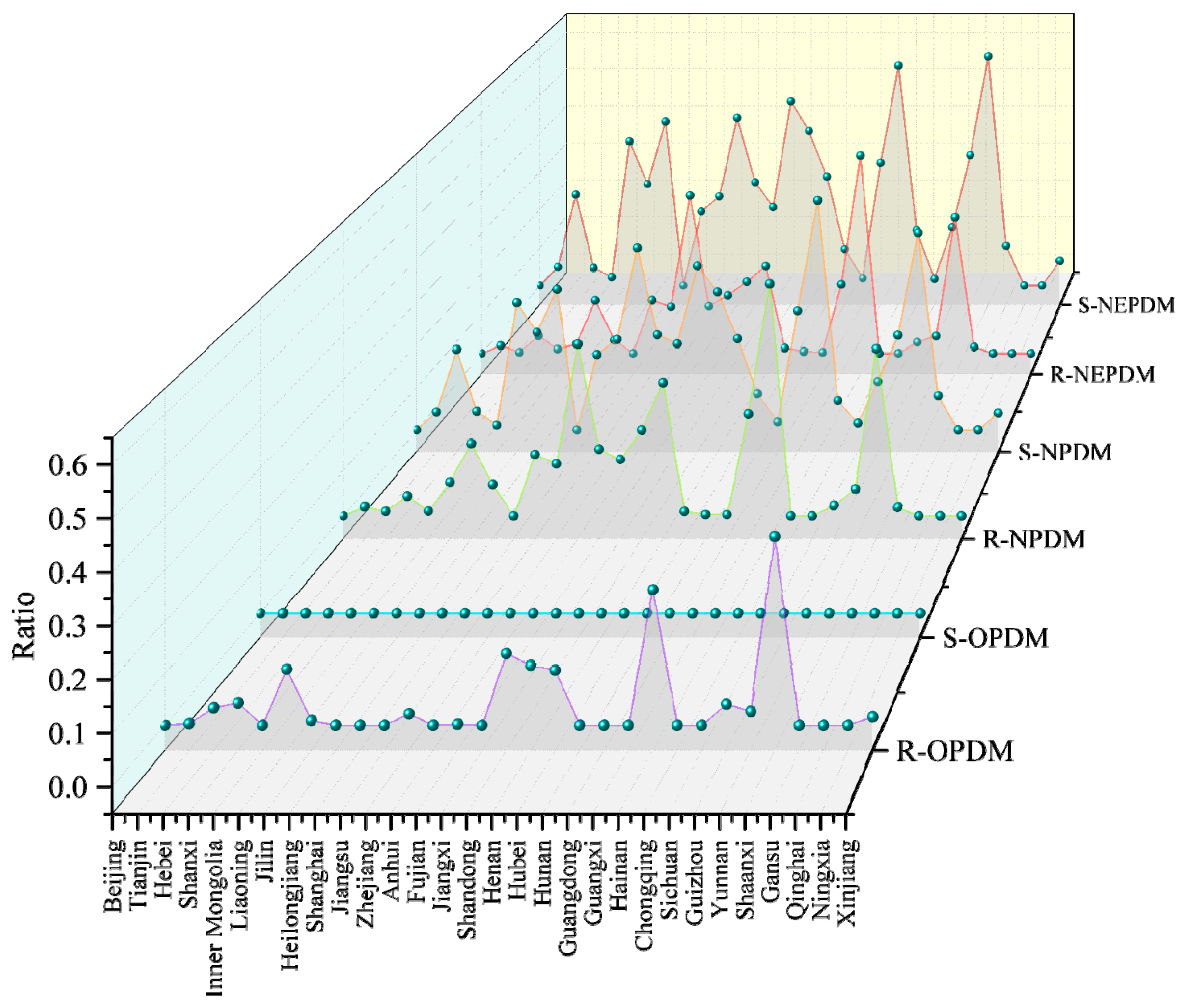
City	R-OPDM	S-OPDM	R-NPDM	S-NPDM	R-NEPDM	S-NEPDM
Beijing	0.00	0.00	0.00	0.00	0.00	0.00
Tianjin	0.00	0.00	0.02	0.04	0.02	0.05
Hebei	0.03	0.00	0.01	0.19	0.00	0.24
Shanxi	0.04	0.00	0.04	0.04	0.04	0.05
Inner Mongolia	0.00	0.00	0.01	0.01	0.01	0.02
Liaoning	0.11	0.00	0.07	0.30	0.02	0.38
Jilin	0.01	0.00	0.16	0.23	0.13	0.27
Heilongjiang	0.00	0.00	0.07	0.33	0.03	0.43
Shanghai	0.00	0.00	0.00	0.00	0.00	0.00
Jiangsu	0.00	0.00	0.14	0.18	0.13	0.19
Zhejiang	0.02	0.00	0.11	0.21	0.12	0.23
Anhui	0.00	0.00	0.38	0.43	0.39	0.44
Fujian	0.00	0.00	0.15	0.22	0.12	0.27
Jiangxi	0.00	0.00	0.12	0.20	0.14	0.21
Shandong	0.14	0.00	0.19	0.38	0.18	0.48
Henan	0.12	0.00	0.29	0.32	0.22	0.41
Hubei	0.11	0.00	0.01	0.21	0.01	0.29
Hunan	0.00	0.00	0.00	0.09	0.00	0.09
Guangdong	0.00	0.00	0.00	0.02	0.00	0.02
Guangxi	0.00	0.00	0.23	0.28	0.17	0.32
Hainan	0.26	0.00	0.51	0.54	0.49	0.58
Chongqing	0.00	0.00	0.00	0.07	0.00	0.14
Sichuan	0.00	0.00	0.00	0.02	0.00	0.02
Guizhou	0.04	0.00	0.02	0.11	0.03	0.15
Yunnan	0.03	0.00	0.06	0.22	0.04	0.34
Shaanxi	0.36	0.00	0.37	0.46	0.34	0.60
Gansu	0.00	0.00	0.02	0.08	0.02	0.10
Qinghai	0.00	0.00	0.00	0.00	0.00	0.00
Ningxia	0.00	0.00	0.00	0.00	0.00	0.00
Xinjiang	0.02	0.00	0.00	0.04	0.00	0.06

Note: The results in Table 3 are derived from new extended DDF models proposed in this paper.

:

In order to further compare the potential of carbon emission reductions in different areas, we draw the data on carbon emission reduction potential into Figure 3 and Figure 4, as shown below.

As shown in Figure 3, based on the original endogenous model, there are six new extended DDF models. Obviously, the carbon emission reduction potential of ECM₁ is higher than that of ECM₂ and CDM. This is because ECM₁ blindly pursues the maximization of economic benefits and ignores the sustainable development of the environment. Therefore, under ECM₁, the overall level of carbon emission reduction is backward, and there is much room for improvement. In other words, the emission reduction potential of each province under ECM₁ is great. Meanwhile, it also reflects that ECM₂ and CDM are more conducive to the sustainable development of the environment. In the ECM₁ model, Heilongjiang, Jiangxi, Chongqing, and Gansu have the greatest development potential, which shows that the current emission reduction technologies in these areas are poor. And compared with the technologically advanced areas, there is still much room for improvement in emission reduction technologies. On the contrary, Beijing and Zhejiang have the smallest ratio of maximum carbon emissions, indicating that the current carbon emission technology in these areas is high. In addition, from the aspect of environmental development, the emission reduction potential of ECM₂ and CDM tends to be the same, which is because both of them take environmental development factors into account, rather than focusing only on economic development.

Comparing three different priority development models, it can initially reveal that the emission reduction potential of each area in the NEPDM is obviously higher than that in the OPDM and NPDM. And the NPDM is obviously higher than that of the OPDM, which shows the priority development of areas with the best comprehensive efficiency. So, the OPDM model can provide the best areas with as large a score as possible, and other areas’ emissions reduction technologies will be forced to be closer to the best. Then, areas with poor technology may perform better. Therefore, compared with other priority development models, the overall level of emission reduction technologies in each area in the OPDM model is higher, and the upside space is smaller. So, the emission reduction potential is smaller. Moreover, in the OPDM model, Shaanxi, Inner Mongolia, Gansu, Ningxia, and Xinjiang have the highest emission reduction potential. In the NPDM model, Shanxi, Inner Mongolia, Guizhou, and Ningxia have the highest emission reduction potential. In the NEPDM model, Shanxi, Shandong, Guizhou, Ningxia, and Xinjiang have the highest emission reduction potential. Meanwhile, it can be seen that the emission reduction potentials of the three priority development models are slightly different, but most of the areas with a greater emission reduction potential are underdeveloped areas, which indicates that the current emission reduction technologies in these areas are relatively low, and there is a gap with those in developed areas. By improving the emission reduction technologies, the carbon emission level can be significantly improved.

As shown in Figure 4, based on the OPDM, NPDM, and NEPDM priority development models, combined with slack variables, six models are extended. Obviously, all areas in the S-NEPDM have the highest emission reduction potential, followed by the S-NPDM, which means that these two models can better highlight the differences in carbon emission reduction in different areas. In the S-NEPDM, Heilongjiang, Shandong, Anhui, Hainan, and Shaanxi have high emission reduction potentials. In the S-NPDM, Anhui, Hainan, and Shaanxi have higher emission reduction potentials. In contrast, the emission reduction potential of each region in the R-NPDM and R-NEPDM is small. In the R-NPDM, Anhui, Henan, Hainan, and Shaanxi have higher emission reduction potentials. In the R-NEPDM, Anhui, Hainan, and Shaanxi have great emission reduction potential. It can be clearly found that the emission reduction potential of the above four expansion models is different, but the peak emission reduction potential is low, and it is concentrated in several areas.

However, the emission reduction potential of each area in S-OPDM is zero, and also, the emission reduction potential of each area in R-OPDM is low, which means that the OPDM model reduces the gap between each area and the optimal carbon emission area and improves the overall emission reduction level. After expansion with slack variables, the improvement value of each area is zero, which shows that each area in the model is on the weak or effective frontier. In the R-OPDM, Shaanxi, Hainan, and Shandong have great emission reduction potential.

4.3. Comparison of Economic Growth Potential Under Extended DDF Models

Based on the extended DDF models proposed in Section 3, using different extended DDF models to choose a reasonable direction and then calculating the maximum economic growth ratio, the formula is as follows:

$$\begin{array}{l}{\displaystyle \frac{\Delta y_i}{y_i}}={\displaystyle \frac{{\displaystyle \sum _{t=2005}^{2019}{\beta }_{it}{\alpha }_{it}\ast y_{it}+S^{+}}}{{\displaystyle \sum _{t=2005}^{2019}{y}_{it}}}}\\ \end{array}$$

(17)

In Formula (17), the denominator represents the maximum amount of GDP increase from 2005 to 2019, and the molecule represents the actual amount of GDP from 2005 to 2019. We take the maximum ratio of GDP growth as the economic growth potential. The greater the maximum ratio of GDP that can be increased, the greater the economic growth potential. On this basis, the basic data of different areas in China are analyzed, and the maximum economic growth ratio in 30 provinces can be obtained, as shown in

Table 4. Economic growth potential of extended DDF models based on endogenous model.

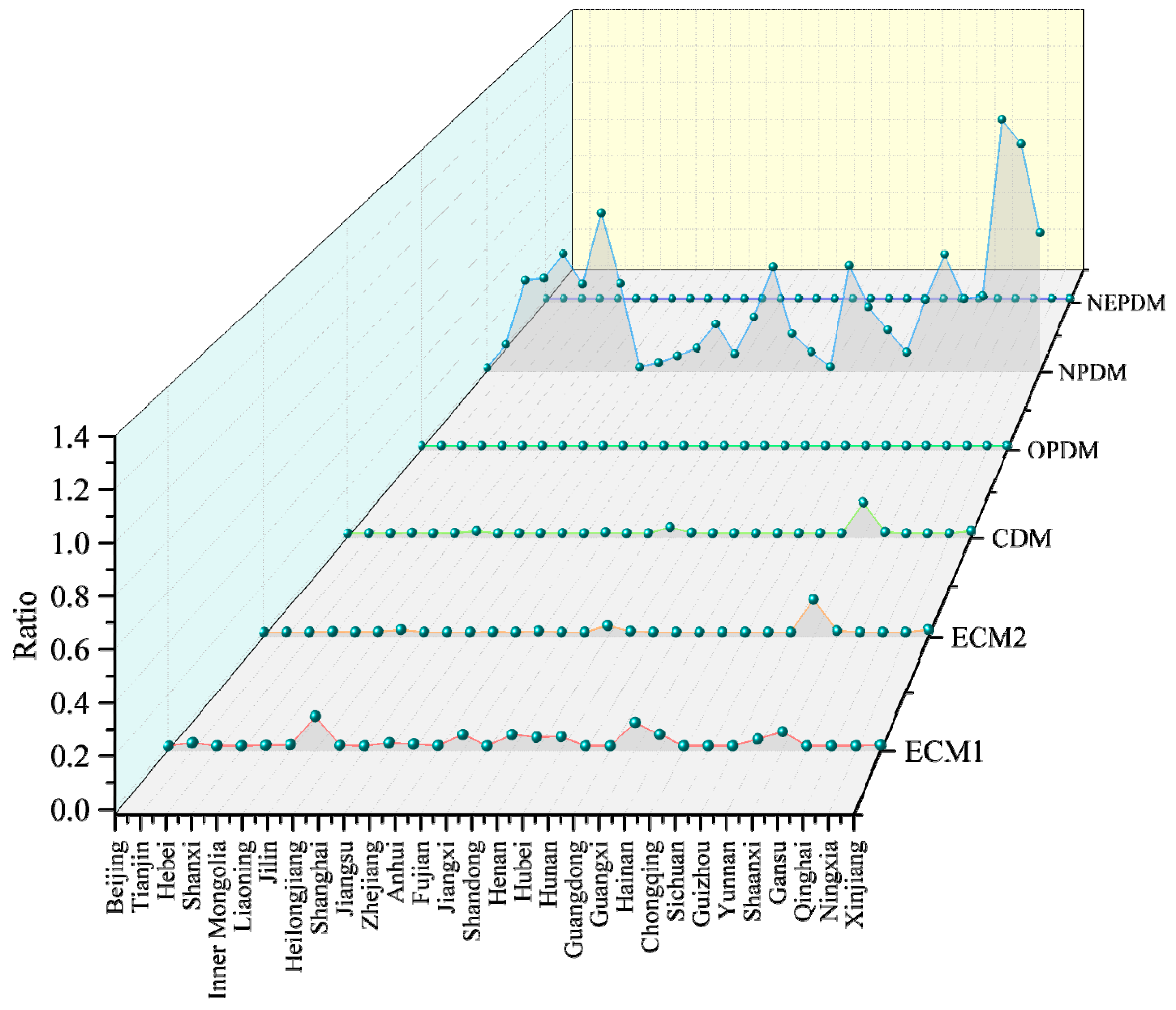
City	DDF	ECM1	ECM2	CDM	OPDM	NPDM	NEPDM
Beijing	0.00	0.00	0.00	0.00	0.00	0.00	0.00
Tianjin	0.12	0.01	0.00	0.00	0.00	0.12	0.00
Hebei	0.43	0.00	0.00	0.00	0.00	0.44	0.00
Shanxi	0.45	0.00	0.00	0.00	0.00	0.45	0.00
Inner Mongolia	0.57	0.00	0.00	0.00	0.00	0.57	0.00
Liaoning	0.42	0.00	0.00	0.00	0.00	0.42	0.00
Jilin	0.77	0.12	0.01	0.01	0.00	0.77	0.00
Heilongjiang	0.42	0.00	0.00	0.00	0.00	0.42	0.00
Shanghai	0.00	0.00	0.00	0.00	0.00	0.00	0.00
Jiangsu	0.03	0.01	0.00	0.00	0.00	0.03	0.00
Zhejiang	0.06	0.01	0.00	0.00	0.00	0.06	0.00
Anhui	0.10	0.00	0.00	0.00	0.00	0.10	0.00
Fujian	0.22	0.04	0.00	0.00	0.00	0.22	0.00
Jiangxi	0.07	0.00	0.00	0.00	0.00	0.07	0.00
Shandong	0.26	0.04	0.00	0.00	0.00	0.26	0.00
Henan	0.51	0.03	0.03	0.03	0.00	0.51	0.00
Hubei	0.17	0.04	0.00	0.00	0.00	0.17	0.00
Hunan	0.08	0.00	0.00	0.00	0.00	0.08	0.00
Guangdong	0.00	0.00	0.00	0.00	0.00	0.00	0.00
Guangxi	0.51	0.09	0.00	0.00	0.00	0.51	0.00
Hainan	0.31	0.05	0.00	0.00	0.00	0.31	0.00
Chongqing	0.19	0.00	0.00	0.00	0.00	0.19	0.00
Sichuan	0.08	0.00	0.00	0.00	0.00	0.08	0.00
Guizhou	0.34	0.00	0.00	0.00	0.00	0.34	0.00
Yunnan	0.57	0.03	0.14	0.14	0.00	0.57	0.00
Shaanxi	0.35	0.06	0.01	0.01	0.00	0.35	0.00
Gansu	0.36	0.00	0.00	0.00	0.00	0.36	0.00
Qinghai	1.25	0.00	0.00	0.00	0.00	1.25	0.00
Ningxia	1.13	0.00	0.00	0.00	0.00	1.13	0.00
Xinjiang	0.67	0.00	0.01	0.01	0.00	0.68	0.00

Note: The results in Table 4 are derived from new extended DDF models and Equation (17) proposed in this paper.

and

Table 5. Economic growth potential of extended DDF models based on priority development model.

City	R-OPDM	S-OPDM	R-NPDM	S-NPDM	R-NEPDM	S-NEPDM
Beijing	0.00	0.00	0.00	0.00	0.00	0.00
Tianjin	0.00	0.00	0.02	0.02	0.01	0.01
Hebei	0.00	0.05	0.17	0.10	0.00	0.00
Shanxi	0.00	0.00	0.00	0.00	0.00	0.00
Inner Mongolia	0.00	0.00	0.02	0.02	0.01	0.00
Liaoning	0.00	0.03	0.27	0.15	0.00	0.01
Jilin	0.01	0.00	0.33	0.30	0.11	0.23
Heilongjiang	0.00	0.02	0.38	0.31	0.00	0.05
Shanghai	0.00	0.00	0.00	0.00	0.00	0.00
Jiangsu	0.00	0.01	0.05	0.03	0.00	0.00
Zhejiang	0.00	0.01	0.09	0.03	0.00	0.00
Anhui	0.00	0.00	0.04	0.02	0.00	0.00
Fujian	0.00	0.01	0.24	0.20	0.00	0.12
Jiangxi	0.00	0.00	0.03	0.01	0.00	0.00
Shandong	0.00	0.03	0.25	0.19	0.00	0.00
Henan	0.03	0.02	0.48	0.48	0.00	0.35
Hubei	0.00	0.00	0.17	0.11	0.00	0.00
Hunan	0.00	0.00	0.05	0.03	0.00	0.00
Guangdong	0.00	0.00	0.00	0.00	0.00	0.00
Guangxi	0.00	0.00	0.46	0.44	0.08	0.34
Hainan	0.00	0.00	0.26	0.25	0.00	0.16
Chongqing	0.00	0.00	0.16	0.11	0.00	0.00
Sichuan	0.00	0.00	0.00	0.00	0.00	0.00
Guizhou	0.00	0.00	0.10	0.09	0.00	0.00
Yunnan	0.14	0.02	0.50	0.49	0.00	0.24
Shaanxi	0.01	0.00	0.34	0.32	0.00	0.01
Gansu	0.00	0.00	0.03	0.03	0.00	0.00
Qinghai	0.00	0.00	0.00	0.00	0.00	0.00
Ningxia	0.00	0.00	0.00	0.00	0.00	0.00
Xinjiang	0.01	0.00	0.06	0.03	0.01	0.00

Note: The results in Table 5 are derived from new extended DDF models and Equation (17) proposed in this paper.

:

In order to further compare the potential of economic growth in different areas, we draw the data on economic growth potential into Figure 5 and Figure 6, as shown below.

From Figure 5, we can clearly see that the overall level of economic development from 2005 to 2019 is high, and it is higher than the level of environmental development (that is, the level of carbon emission reduction). Based on the original endogenous model, there are six new extended DDF models. Obviously, the economic development potential of each area in the NPDM is the highest, followed by ECM₁. In the NPDM, Inner Mongolia, Jilin, Henan, Guangxi, Yunnan, Qinghai, Ningxia, and Xinjiang have great potential for economic growth, which indicates that there is a gap between these areas and economically developed areas, and there is a big room for growth in economic development. The level of economic development can be further improved by means of policy inclination. In the ECM₁, Jilin, Guangxi, and Shaanxi have great economic growth potential. Among the ECM₂ and CDM, Shaanxi has the greatest economic growth potential. However, in the OPDM, the economic growth potential of each region is zero, which is because the model gives priority to the development of areas with higher economic level, and other areas are forced to reduce the gap with the best areas, resulting in a higher overall economic development level, only in economic development, without further improvement.

As shown in Figure 6, based on the OPDM, NPDM, and NEPDM priority development models, combined with slack variables, six models are extended. Obviously, the economic growth potential of the R-NPDM is the largest, followed by the S-NPDM, which implies that these two models can initially reveal the differences in economic growth in different areas. In the R-NPDM, Henan, Guangxi, and Yunnan have great economic growth potential. In the S-NPDM, Henan, Guangxi, and Yunnan have great economic growth potential, which is consistent with the R-NPDM model, but the economic growth potential is slightly different. In addition, the economic growth potential of each area in the R-NEPDM and S-NEPDM is in the middle. In the R-NEPDM, Jilin and Guangxi have great potential for economic growth. In the S-NEPDM, Jilin, Henan, Yunnan, and Guangxi have great economic growth potential. However, the economic growth potential of each region in the S-OPDM and R-OPDM is low. In the S-OPDM, Liaoning and Yunnan have great potential for economic growth. In the R-OPDM, Henan and Yunnan have great economic growth potential. Compared with Russian regional economic models [30], it only analyzes the economic growth differences of different regions in Russia. In contrast, the models in this study further analyze economic growth between different regions, which provides a more abundant reference for policy makers.

Moreover, combined with Figure 4, the carbon emission reduction potential and economic growth potential of Beijing, Tianjin, Shanxi, Inner Mongolia, Jilin, Shanghai, Anhui, Jiangxi, Hubei, Hunan, Guangdong, Hainan, Chongqing, Sichuan, Guizhou, Shaanxi, Gansu, Qinghai, Ningxia, and Xinjiang are all zero, which shows that these areas are all effective for the S-NPDM model. From economic structure, Beijing and Shanghai, as the economic centers of China, have highly shifted their industrial structures to service industries and high-tech industries, and their carbon emission intensity is relatively low. Therefore, the potential of carbon emission reduction in these areas is small. In recent years, by industrial upgrading and technological transformation, Shanxi and Inner Mongolia have optimized their energy structure and reduced carbon emissions to some extent. Regions such as Guangdong and Hubei have gradually transformed into green manufacturing by industrial upgrading and technological innovation. For example, Guangdong has made remarkable progress in the fields of electronic manufacturing and new energy vehicles, reducing the intensity of carbon emissions. The economic development of western regions such as Qinghai and Ningxia is relatively backward, but due to abundant renewable energy resources (such as wind energy and solar energy), their energy structure is relatively clean.

From a policy background, Beijing and Shanghai have implemented strict environmental protection policies and carbon emission reduction measures, such as promoting clean energy and restricting the development of highly polluting industries. These policies have significantly improved energy efficiency and further reduced the potential for carbon emission reduction. The government has issued a series of transformation policies for regions such as Shanxi and Inner Mongolia, including support for clean energy development and the elimination of outdated production capacities. These measures have fully tapped the potential of carbon emission reduction in these regions. Regions such as Guangdong and Hubei have actively responded to the national “double carbon” goals, such as the carbon trading pilot and green financial support, which further reduced carbon emissions. The government has vigorously promoted renewable energy projects in western regions, such as Qinghai and Ningxia, and implemented an ecological compensation mechanism. As a result, these regions have relatively low levels of carbon emissions, and thus, their potential for further carbon emission reduction is limited.

4.4. Comparison of Improved Path Under Extended DDF Models

As shown in Figure 7, compared with the CDM model, the S⁻ in the ECM₂ model needs to be improved. That is, the development mode of environmental concern can better reveal the improvement path of environmental development. Combining Figure 7 and Figure 8, at the economic level, the range and quantity of improvement in different models are smaller than that for carbon emission reduction. In different DDF expansion models, S⁻ and S⁺ of the R-OPDM and CDM models need not be improved, which means that these two models tend to coordinate the development of the economy and environment in various regions and focus on improving the overall development level. In these two models, the economic development level and the carbon emission level of each region are at least at the frontier of weak effective production.

In addition, combined with the analysis of S-NPDM in Figure 4 and Figure 6, we find that Shanxi, Anhui, Jiangxi, Hubei, Hunan, Chongqing, Sichuan, Guizhou, Shaanxi, and Gansu are weakly effective DMUs because the values of the improvement directions in these areas do not affect the improvement path, but their relaxation variable values are not all zero. Then, they can improve this situation by adjusting the input–output value according to the relaxation value. Moreover, Beijing, Tianjin, Inner Mongolia, Jilin, Shanghai, Jiangxi, Guangdong, and Hainan are effective DMUs without any improvement.

Meanwhile, at the level of carbon emissions, the S-NEPDM has the highest emission reduction potential, and at the level of economic development, the R-NPDM has the highest economic development potential. On this basis, the quantity and range of S⁺ in S-NEPDM are greater than those in other models. Moreover, the quantity and range of S⁻ in the R-NPDM are also greater than those in the other models, which further proves that the carbon emission reduction potential is directly proportional to the slack variables. That is, the greater the emission reduction potential, the greater the scope for improvement.

This paper found that the level of economic–environmental sustainable development in China exhibits significant spatial heterogeneity, which is consistent with the conclusions of some studies about the globe [30,31]. That is, there is a nonlinear relationship between economic development level and environmental quality. Furthermore, this paper further reveals the key role of policy intervention and technological progress in promoting economic–environmental sustainable development, which is consistent with the relevant recommendations in the Global Sustainable Development Goals (SDGs).

5. Conclusions

This paper extends and popularizes the DDF model by introducing an endogenous direction selection mechanism, systematically analyzing the carbon reduction potential under various economic–environmental development modes, including economic concern, environmental concern, coordinated development, and priority development. The conclusions are as follows:

Optimizing the emission reduction effect: The results of this paper show that the carbon emission reduction potential is directly proportional to the slack variables. That is, the greater the emission reduction potential, the greater the scope for improvement. This provides an important basis for policy makers. When formulating emission reduction policies, priority should be given to those areas with great emission reduction potential, and the emission reduction effect should be maximized by optimizing resource allocation and technological innovation.

Formulate differentiated emission reduction strategies: First, the carbon emission reduction potential of the ECM₁ is higher than that of the ECM₂ and CDM, and the emission reduction potential of the NEPDM is higher than in other priority development models. Second, all areas in the S-NEPDM have the highest emission reduction potential, followed by the S-NPDM, which means that these two models can better highlight the differences in carbon emission reduction in different areas. The R-NPDM and R-NEPDM are concentrated in several areas. Moreover, the OPDM model reduces the gap between each area and the optimal carbon emission area and improves the overall emission reduction level. The above conclusions provide a scientific basis for the formulation of differentiated emission reduction strategies. In the areas where the S-NEPDM and S-NPDM are outstanding, high-intensity emission reduction measures can be prioritized. In the areas where the R-NPDM and R-NEPDM are concentrated, region-specific emission reduction policies can be designed in a targeted manner. The application of the OPDM model can help backward areas narrow the gap with advanced areas and promote the overall emission reduction level.

Balanced economic–environmental development: While pursuing economic growth, the S-NEPDM model can be utilized to optimize emission reduction pathways, achieving a win–win situation for both the economy and environment. In areas with significant economic development potential, the R-NPDM model can be prioritized to promote green economic growth. For areas that have already achieved an efficient state (such as some DMUs in the S-NPDM model), it can be used as a benchmark to disseminate its successful experiences.

Promote green economic growth: In areas with great economic development potential (such as areas with outstanding NPDM and R-NPDM), priority can be given to promoting a green economic growth mode and achieving sustainable development through technological innovation and industrial upgrading. In areas with relatively backward economic development, policy incentives and technical support can be employed to gradually narrow the gap with more advanced areas. By popularizing the S-NPDM model, a balance can be obtained between economic development and environmental protection, thus realizing regional coordinated development.

This paper only considers a static sustainable development analysis. In the future, we can explore a dynamic multi-objective optimization model, consider the interaction between the economy and environment in a time series, and simultaneously include multi-dimensional goals, such as carbon emissions, economic development, and social equity, so as to further enhance the comprehensiveness and applicability of the study. In addition, Future research can further combine the relevant data from the United States, Japan, South Korea, and the European Union and make a cross-border comparative analysis to verify the applicability of these models in different economic backgrounds.

References

- Daniel, A.; Du, J.G.; Stephen Ntiri, A.; Agnes, A. Energy generation and carbon dioxide emission-The role of renewable energy for green development. Energy Rep. 2024, 12, 1420–1430. [Google Scholar]
- Pittman, R.W. Multilateral productivity comparisons with undesirable outputs. Econ. J. 1983, 93, 883–891. [Google Scholar] [CrossRef]
- Stergiou, E. The effect of heterogeneity on environmental efficiency: Evidence from European industries across sectors. J. Clean. Prod. 2024, 441, 141036. [Google Scholar] [CrossRef]
- Lozano, S.; Gutiérrez, E.; Aguilera, E. Environmental efficiency of rainfed and irrigated wheat crops in Spain. A stochastic DEA metafrontier approach. OR Spectr. 2024. [Google Scholar] [CrossRef]
- Chung, Y.H.; Färe, R.; Grosskopf, S. Productivity and undesirable outputs: A directional distance function approach. J. Environ. Manag. 1997, 51, 229–240. [Google Scholar] [CrossRef]
- Chambers, R.; Chung, Y.H.; Färe, R. Profit, Directional distance functions, and Nerlovian efficiency. J. Optim. Theory Appl. 1998, 98, 351–364. [Google Scholar] [CrossRef]
- Yao, Y.; Bi, X.; Li, C.H.; Xu, X.H.; Jing, L.; Chen, J.L. A united framework modeling of spatial-temporal characteristics for county-level agricultural carbon emission with an application to Hunan in China. J. Environ. Manag. 2024, 364, 121321. [Google Scholar] [CrossRef]
- Zhang, Y.; Xu, X.Y. Carbon emission efficiency measurement and influencing factor analysis of nine provinces in the Yellow River basin: Based on SBM-DDF model and Tobit-CCD model. Environ. Sci. Pollut. Res. 2022, 29, 33263–33280. [Google Scholar] [CrossRef]
- Li, Z.W.; Zhang, C.J.; Zhou, Y. Spatio-temporal evolution characteristics and influencing factors of carbon emission reduction potential in China. Environ. Sci. Pollut. Res. 2021, 28, 59925–59944. [Google Scholar] [CrossRef]
- Chen, Y.; Pan, Y.B.; Ding, T.; Wu, H.Q.; Deng, G.W. A three-level meta-frontier directional distance function approach for carbon emission efficiency analysis in China: Convexity versus non-convexity. Int. J. Prod. Res. 2024, 62, 6493–6517. [Google Scholar] [CrossRef]
- Teng, M.M.; Ji, D.D.; Han, C.F.; Liu, P.H. Optimizing the Allocation of CO2 Emission Rights in the Yangtze River Delta City Agglomeration Region of China Based on Equity, Efficiency and Sustainability. Int. J. Environ. Res. 2025, 19, 29. [Google Scholar] [CrossRef]
- Ma, C.B.; Hailu, A.; You, C.Y. A critical review of distance function based economic research on China’s marginal abatement cost of carbon dioxide emissions. Energy Econ. 2019, 84, 104533. [Google Scholar] [CrossRef]
- Chen, L.; Wang, Y.M. Game directional distance function in meta-frontier data envelopment analysis. Omega 2023, 121, 102935. [Google Scholar] [CrossRef]
- Gulati, R. Global and local banking crises and risk-adjusted efficiency of Indian banks: Are the impacts really perspective-dependent? Q. Rev. Econ. Financ. 2022, 84, 23–29. [Google Scholar] [CrossRef]
- Barbero, J.; Zofío, J.L. The measurement of profit, profitability, cost and revenue efficiency through data envelopment analysis: A comparison of models using BenchmarkingEconomicEfficiency.jl. Socio-Econ. Plan. Sci. 2023, 89, 101656. [Google Scholar] [CrossRef]
- Nepomuceno, T.C.C.; Agasisti, T.; Bertoletti, A.; Daraio, C. Multicriteria panel-data directional distances and the efficiency measurement of multidimensional higher education systems. Omega 2024, 125, 103044. [Google Scholar] [CrossRef]
- Wu, F.; Ji, D.J.; Zha, D.L.; Zhou, D.Q.; Zhou, P. A nonparametric distance function approach with endogenous direction for estimating marginal abatement costs of CO2 emissions. J. Manag. Sci. Eng. 2022, 7, 330–345. [Google Scholar] [CrossRef]
- Wang, A.L.; Hu, S.; Li, J.L. Using machine learning to model technological heterogeneity in carbon emission efficiency evaluation: The case of China’s cities. Energy Econ. 2022, 114, 106238. [Google Scholar] [CrossRef]
- Färe, R.; Grosskopf, S.; Lovell, C.; Pasurka, C. Multilateral Productivity Comparisons When Some Outputs are Undesirable: A nonparametric Approach. Rev. Econ. Stat. 1989, 71, 90–98. [Google Scholar] [CrossRef]
- Kaneko, S.; Fujii, H.; Sawazy, N.; Fjikura, R. Financial allocation strategy for the regional pollution abatement cost of reducing sulfur dioxide emissions in the thermal power sector in China. Energ. Policy 2010, 38, 2131–2141. [Google Scholar] [CrossRef]
- Färe, R.; Grosskopf, S.; Whittaker, G. Directional output distance functions: Endogenous directions based on exogenous normalization constraints. J. Prod. Anal. 2013, 40, 267–269. [Google Scholar] [CrossRef]
- Hampf, B.; Krüger, J.J. Optimal directions for directional distance functions: An exploration of potential reductions of greenhouse gases. Am. J. Agric. Econ. 2015, 97, 920–938. [Google Scholar] [CrossRef]
- Chien, F.S.; Anwar, A.; Hsu, C.C.; Sharif, A.; Razzaq, A.; Sinha, A. The role of information and communication technology in encountering environmental degradation: Proposing an SDG framework for the BRICS countries. Technol. Soc. 2021, 65, 101587. [Google Scholar] [CrossRef]
- Liang, L.; Wu, J.; Cook, W.D.; Zhu, J. Alternative secondary goals in DEA cross-efficiency evaluation. Int. J. Prod. Econ. 2008, 113, 1025–1030. [Google Scholar] [CrossRef]
- Troutt, M.D. Derivation of the maximin efficiency ratio model from the maximum decisional efficiency principle. Ann. Oper. Res. 1997, 73, 323–338. [Google Scholar] [CrossRef]
- Xu, G.C.; Wu, J.; Zhu, Q.Y.; Pan, Y.H. Fixed cost allocation based on data envelopment analysis from inequality aversion perspectives. Eur. J. Oper. Res. 2024, 313, 281–295. [Google Scholar] [CrossRef]
- Chen, F.; Zhao, T.; Xia, H.M.; Cui, X.Y.; Li, Z.Y. Allocation of carbon emission quotas in Chinese provinces based on Super-SBM model and ZSG-DEA model. Clean Technol. Environ. Policy 2021, 23, 2285–2301. [Google Scholar] [CrossRef]
- Zhang, J.X.; Jin, W.X.; Yang, G.L.; Li, H.; Ke, Y.J.; Philbin, S.P. Optimizing regional allocation of CO2 emissions considering output under overall efficiency. Socio-Econ. Plan. Sci. 2021, 77, 101012. [Google Scholar] [CrossRef]
- Wang, R.Z.; Hao, J.X.; Wang, C.A.; Tang, X.; Yuan, X.Z. Embodied CO2 emissions and efficiency of the service sector: Evidence from China. J. Clean. Prod. 2020, 247, 119116. [Google Scholar] [CrossRef]
- Mikheeva, N. Qualitative Aspect of the Regional Growth in Russia: Inclusive Development Index. Reg. Sci. Policy Pract. 2020, 12, 611–626. [Google Scholar] [CrossRef]
- Andreica, R.; Jaradat, M. Analysis of economic development and sustainable development of Romania. Metal. Int. 2011, 16, 9–12. [Google Scholar]