Optimization of Renewable Energy Sharing for Electric Vehicle Integrated Energy Stations and High-Rise Buildings Considering Economic and Environmental Factors

Abstract

Amid the rapid growth of the new energy vehicle industry and the accelerating global shift toward green and low-carbon energy alternatives, this paper develops a multi-objective optimization model for an Electric Vehicle Integrated Energy Station (EVIES) and a high-rise building wind-solar-storage sharing system. The model aims to maximize the daily economic revenue of the EVIES, minimize the load variance on the grid side of the building, and reduce overall carbon emissions. To solve this multi-objective optimization problem, a Multi-Objective Sand Cat Swarm Optimization Algorithm (MSCSO) based on a mutation-dominated selection strategy is proposed. Benchmark tests confirm the significant performance advantages of MSCSO in both solution quality and stability, achieving the optimal mean and minimum variance in 73% of the test cases. Further comparative analyses validate the effectiveness of the proposed system, showing that the optimized configuration increases daily economic revenue by 26.54% on average and reduces carbon emissions by 37.59%. Additionally, post-optimization analysis reveals a smoother load curve after grid integration, a significantly reduced peak-to-valley difference, and improved overall operational stability.

1. Introduction

As industrialization and urbanization accelerate, over-reliance on fossil energy has led to the gradual depletion of traditional energy sources and triggered global climate change. Therefore, promoting clean energy development and reducing carbon emissions have become the keys to achieving energy sustainability and mitigating environmental pollution [1,2]. In this scenario, alternative energy sources like hydropower, solar photovoltaics, and wind energy, with their abundant potential, have increasingly become key options for substituting conventional energy and reducing carbon emissions. In recent years, countries have actively promoted renewable energy by expanding installed capacity and generation, while adopting innovative system designs, new materials, and low-carbon technologies. These efforts aim to enhance energy efficiency and sustainability, supporting the transition to a greener energy structure. Meanwhile, the effective integration of electric vehicles and building energy systems with renewable energy, as key areas of energy utilization and consumption, is becoming an important direction in promoting the green transformation of energy. Therefore, optimizing renewable energy utilization and balancing economic efficiency with environmental sustainability through the synergy of electric vehicle charging and discharging with building energy complementary systems has become a key focus of future research and practice.

In recent years, with the advancement of the global energy transition, many scholars have achieved remarkable results in renewable energy utilization, electric vehicle charging and discharging, and the optimization of building energy complementary systems. To optimize the utilization of renewable energy, scholars have proposed various methods to enhance the operational efficiency, economic benefits, and environmental sustainability of energy systems. Sun et al. [3] explored strategies to improve the operational efficiency of fast charging stations by integrating renewable energy with battery storage. They applied the Multi-Objective Particle Swarm Optimization algorithm (MOPSO)and the Technique for Order Preference by Similarity to Ideal Solution methods (TOPSIS) to optimize energy dispatch and enhance the utilization of intermittent power generation. Liao et al. [4] introduced an optimization framework for an integrated energy station incorporating photovoltaic generation and energy storage. Their approach sought to efficiently manage electric vehicle charging while reducing losses in the energy storage system. Shen et al. [5] introduced a capacity configuration strategy for integrated energy systems (IES) based on cooling-to-heat and heat-to-electricity principles, demonstrating its feasibility through seasonal case studies. Regarding Electric Vehicle (EV) charging and discharging systems, research has focused on optimizing station layouts, resource allocation, and scheduling strategies, focusing on economic efficiency and green energy dispatch. Zhang et al. [6] proposed a green adaptive scheduling model for battery swap station clusters (BSSCs) to optimize charging and discharging costs and green energy utilization. Yang et al. [7] focused on the uneven distribution of batteries and established an adaptive response model to optimize battery distribution and replacement. On the other hand, Zhang et al. [8] proposed a charging station siting and capacity optimization model to adapt to dynamic charging demand. In addition, in terms of complementary building energy systems, Yu Qian Ang [9] introduced an optimization approach utilizing the Urban Building Energy Model (UBEM) to design a diversified renewable energy system for a coastal community. This study examined the composition of renewable sources to fulfill year-round energy needs, while addressing technological and economic constraints. Alper Çiçek [10] proposed a multi-objective hydrogen-based residential community target energy management model. Ge et al. [11] investigated the complementarity of rooftop photovoltaic wind turbine hybrid generation systems and their matching with building energy demand. These studies explored how to improve the matching between renewable energy sources and building energy demand, and indirectly provided theoretical support for the optimal design of complementary building energy systems. Although the above studies have made significant progress in several areas, the effective integration of EV fast-charging stations and the construction of energy-complementary systems to fully utilize the potential of renewable energy sources for more efficient and environmentally friendly energy use remain key directions for future research. Enhancing the coordinated operation of these systems to achieve greater economic and environmental benefits remains a key challenge for researchers. To this end, this paper proposes a multi-objective capacity allocation optimization model covering wind power, photovoltaic, energy storage systems, electric vehicle swapping/charging/discharging modules, and high-rise building microgrid systems. The model determines the optimal installed capacity of each system component through a multi-objective optimization. Based on this, the optimal operation schemes of wind power, PV, and energy storage systems to maximize the daily economic benefits and minimize the grid-side load variance and comprehensive carbon emissions to enhance the system’s overall synergistic benefits are determined.

In recent years, significant advancements in multi-objective optimization algorithms have enhanced their capabilities for solving complex problems. Researchers have refined solution set distribution, improved high-dimensional problem-solving efficiency, and accelerated convergence by restructuring algorithms, optimizing search strategies, and integrating novel models. Xie et al. [12] proposed a two-stage evolutionary algorithm incorporating fuzzy preference indicators, which effectively improves the solution set of a multi-modal multi-objective optimization problem distribution quality; Shen et al. [13] enhanced the solution efficiency of high-dimensional multi-objective problems through local learning strategies and agent model guidance; Parham Hadikhani et al. [14] introduced Gaussian variants and game theory to achieve automatic clustering optimization, which significantly enhances the global and diverse nature of the solution; Yang et al. [15] combined temporal convolutional networks and adaptive NSGA III algorithm to optimize the multi-objective performance of 5G antenna design; Wei et al. [16] accelerated the convergence of the algorithm through grey prediction and regeneration operators; Gao et al. [17] used Switching Competitive Ensemble Optimizer (SCEA) to learn the irregular Pareto frontier structure; Mohammed Jameel et al. [18] combined the mantis search algorithm with an elite nondominated sorting method to propose a method that balances convergence and optimization that proposed an optimization framework that balances convergence and diversity. On this basis, this paper proposes an MSCSO based on a mutation-dominated selection strategy to further improve the solution performance of multi-objective optimization. The algorithm borrows the local search capability and concise iterative mechanism of the Sand Cat Swarm Optimization Algorithm (SCSO) [19] proposed in 2022. It replaces the genetic algorithm (GA) component of the original NSGA-III framework. The selection, crossover, and mutation operations of the original framework are replaced by introducing a strategy that combines positional mutation with the judgment of non-dominance relationships. This strategy not only enhances the local search capability and computational efficiency by perturbing the solution set through position mutation and filtering the superior solutions by combining with dominance relations, but also effectively improves the distribution quality of the solution set to make it closer to the Pareto frontier.

This research is significant for guiding the optimized operation and system capacity allocation of wind-solar-storage sharing systems in EVIES and high-rise buildings. This paper constructs a multi-objective capacity optimization model and determines the installed capacity of each system, providing a theoretical basis for the practical application of the sharing model. The optimized operation results demonstrate how the system enhances the economic returns of the EVIES, reduces building grid load fluctuations, and lowers carbon emissions while balancing economic benefits with environmental sustainability. These results provide important references for advancing the electric vehicle industry and its infrastructure, supporting the green transformation of the energy structure, and contributing to the achievement of the ‘dual-carbon’ goal.

The main contributions of this study are as follows:

(1)

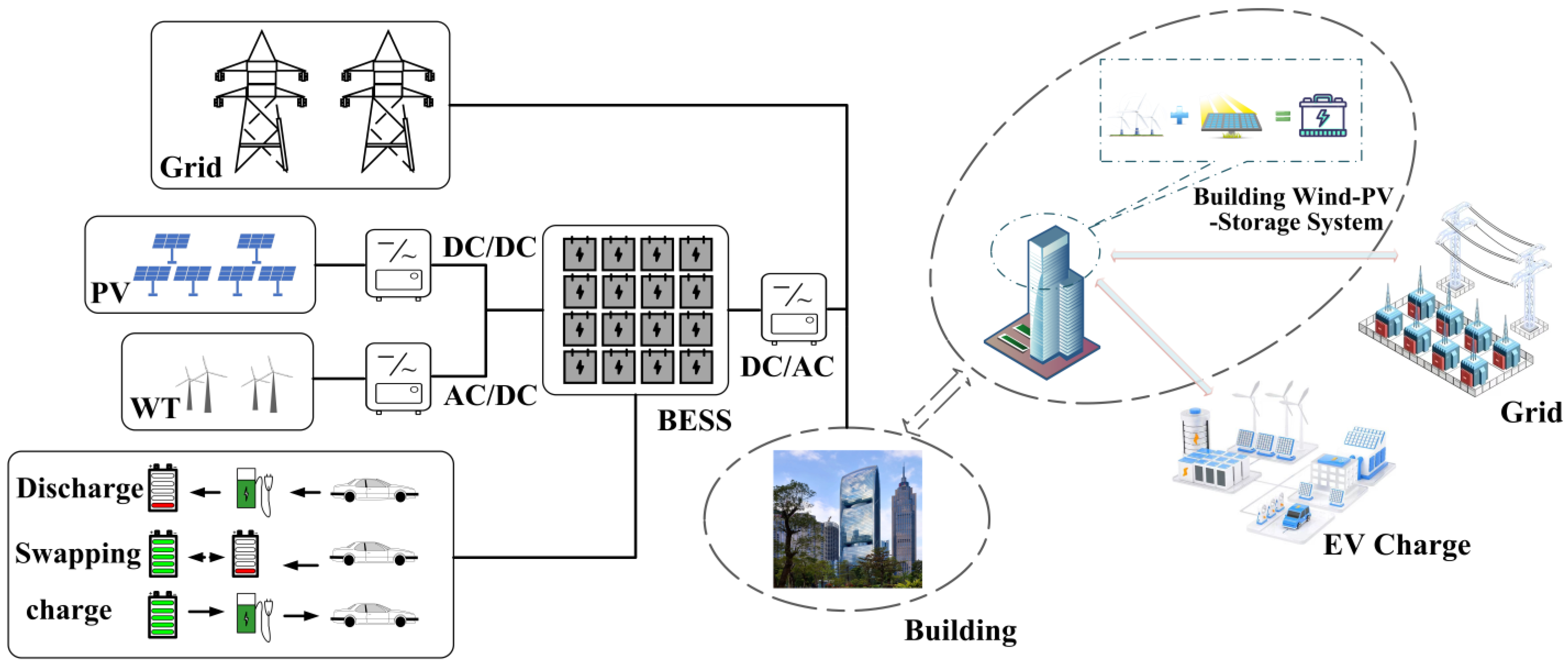
A detailed system model was developed, integrating wind power, photovoltaics, energy storage, EV charging/discharging, and building electricity loads. This model enables the coordination and optimization of energy flow between the EVIES, high-rise building wind-solar-storage sharing system, and power grid, providing a theoretical foundation and technological framework for optimizing capacity allocation.

(2)

A multi-objective capacity allocation optimization model was established, and the entropy-TOPSIS (ETOPSIS) method was applied to optimize the installed capacities of photovoltaic, wind power, and energy storage systems. This optimization significantly improves the system’s economic efficiency, reduces carbon emissions, stabilizes power grid load fluctuations, and achieves a multi-dimensional balance of economy, environmental protection, and stability.

(3)

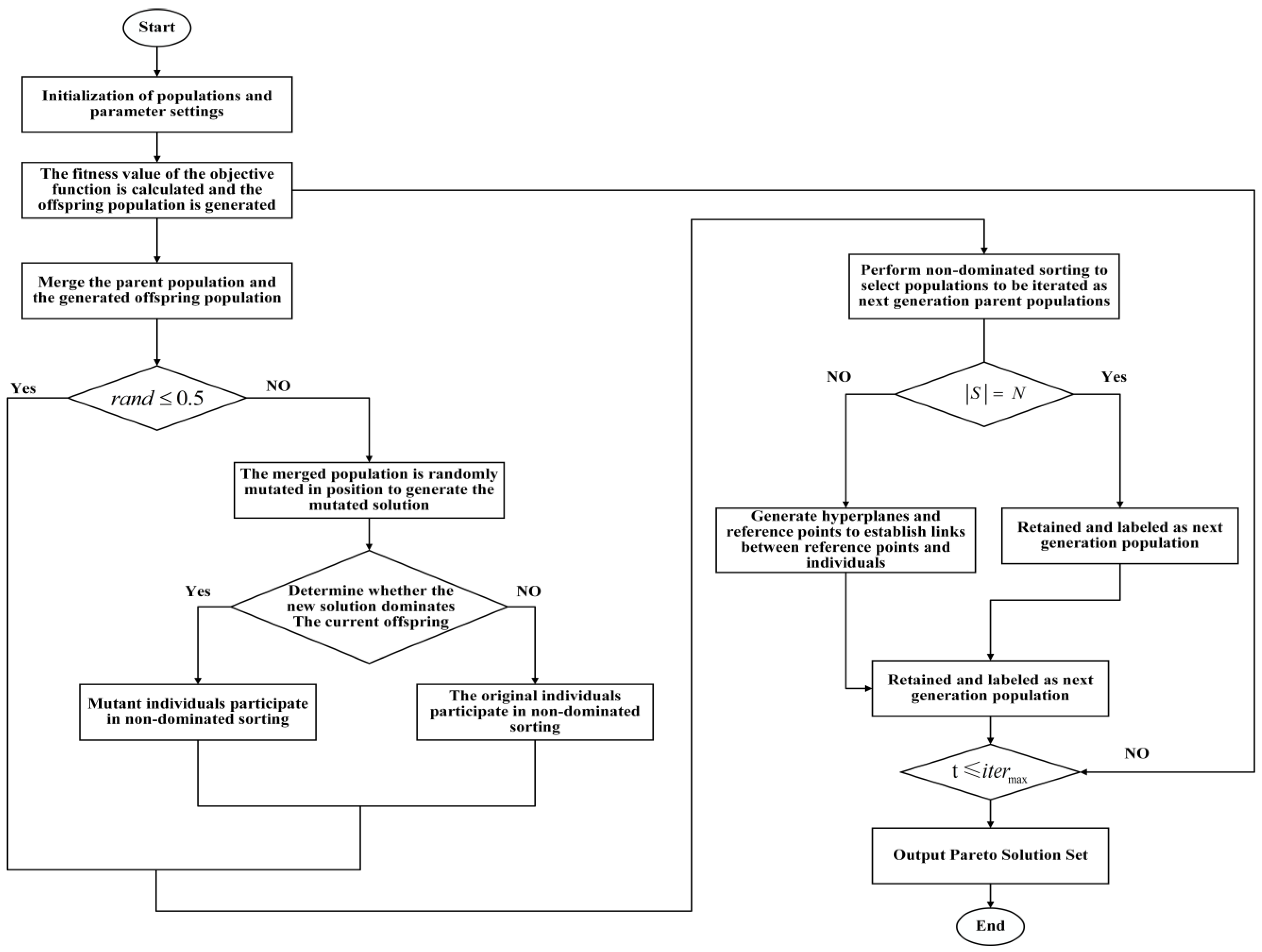
An MSCSO based on a mutation-dominated selection strategy was proposed to effectively solve the optimization model. The simulation results show that MSCSO outperforms existing algorithms in terms of solution efficiency, convergence speed, and solution set diversity, verifying its advantages in multi-objective optimization.

This paper is structured as follows: Section 2 provides an overview of the EVIES and high-rise building wind-solar-storage sharing system model. Section 3 details the mathematical structure of the EVIES and the high-rise building wind-solar-storage sharing system. Section 4 introduces the multi-objective capacity-allocation optimization model. Section 5 describes the MSCSO. Section 6 presents an analysis of the simulation experiment results. Section 7 summarizes this paper and its main contributions.

2. System Description

The EVIES and high-rise building wind-solar-storage sharing system utilize wind and photovoltaic power generation to provide clean energy for electric vehicles and high-rise buildings and facilitate power storage and scheduling via the energy storage system to improve energy utilization efficiency. The system achieves multi-energy complementarity and replaces energy consumption with alternative energy sources through energy conversion equipment, thereby meeting the energy demand of each subsystem. As independent energy production sources, photovoltaic and wind power generation systems first charge the energy storage system of the EVIES and support the charging and discharging needs of electric vehicles. The wind-solar-storage system of a high-rise building prioritizes the building’s electricity load and energy storage battery. When the EVIES discharges and the high-rise building requires charging, its power will be prioritized to supply the building; conversely, when the high-rise building discharges, its power will be prioritized to meet the charging demand of the EVIES. Moreover, the battery energy storage system charges during off-peak or flat periods and discharges during peak periods, thus further improving the economic returns of the EVIES. The EVIES and high-rise building wind-solar-storage sharing system are illustrated in Figure 1. Meanwhile, Figure 2 provides a detailed view of the energy flow and scheduling priorities, highlighting the decision-making process involved in allocating energy to different subsystems based on renewable energy generation, battery status, and real-time demand.

The energy storage system operation mode of the EV charging station is scheduled based on the priorities of EV charging, discharging, and power swap. The system prioritizes meeting the demand for electric vehicle power swaps. When the energy storage system battery is insufficient, electric vehicles that have not undergone a power swap will switch to charging mode. As the charging demand increases, if the total demand for EV charging and discharging in a specific period exceeds the capacity of the system’s charging equipment, the system will prioritize the charging demand and moderately reduce discharging operations. Additionally, to avoid overloading the power grid, the system will reasonably dispatch charging and discharging according to the grid load condition and equipment capacity, ensuring stable grid operation.

3. System Model

3.1. Wind Power Generation Model

The electricity output of a wind turbine is largely determined by the wind speed and design parameters. Since the blades harness kinetic energy from the wind to generate power, wind speed plays a pivotal role in this process [20]. This dependency is mathematically represented by a piecewise function, as reported in Equations (1)–(3).

$$P_{wt}=\left\{\begin{array}{l}0V\le V_{cut-in} ,V\ge V_{cut-out}\\ N_{wt}(V^{3}a-P_{rate-wt}b) V_{cut-in}\le V\le V_{rate}\\ N_{wt}{P}_{rate-wt} V_{rate}\le V\le V_{cut-out}\end{array}\right.$$

(1)

$$\mathrm{a}={\displaystyle \frac{P_{rate-wt}}{V_{rate}^3-V_{cut-in}^3}}, \mathrm{b}={\displaystyle \frac{V_{cut-in}^3}{V_{rate}^3-V_{cut-in}^3}}$$

(2)

$${\displaystyle \frac{V}{V_0}}={\left({\displaystyle \frac{Z}{Z_0}}\right)}^{\phi }$$

(3)

where $N_{wt}$ is the number of wind turbines; $P_{rate-wt}$ is the rated power of the wind turbine, 10 kW; $V_{cut-in}$ is the cut-in wind speed, 3 m/s; $V_{cut-out}$ is the cut-out wind speed, 20 m/s; $V_{rate}$ is the rated wind speed, 12 m/s; $V$ is the wind speed at the hub height of $Z$, m/s; $V_0$ is the measured height of $Z_0$, m/s; $Z_0$ is the measured height, $Z$ is the hub height of the wind turbine, 15 m; $\phi$ is the ground surface friction coefficient, for the open ground, take 1/7.

3.2. Photovoltaic Power Generation Model

Photovoltaic systems convert solar radiation into electricity using the photovoltaic effect. The output power varies with factors like solar irradiance and ambient temperature, and the following equation (Equation (4)) represents the power output of the PV array [21].

$$P_{pv}=\left\{\begin{array}{l}{N}_{pv}{l}_{pv}{\displaystyle \frac{G_R}{G_{RSI}}}\times [1+\lambda (T_R-T_{RIS})] G_R<G_{RSI} \\ N_{pv} G_R\ge G_{RSI} \end{array}\right.$$

(4)

where $P_{pv}$ for the actual power of photovoltaic cells; $N_{pv}$ for the installed capacity of photovoltaic power generation equipment; $G_R$ for the actual light intensity; $l_{pv}$ for the standard conditions (light radiation intensity $G_{RSI}=1000 {\mathrm{W}/\mathrm{m}}^2$, temperature $T_{RIS}=25 °\mathrm{C}$) of the distributed photovoltaic rated output; $\lambda$ that the power temperature coefficient (generally take $0.0039 °{\mathrm{C}}^{-1}$); $T_R$ that the actual surface temperature of the battery; $T_{RIS}$ that the battery’s rated temperature.

3.3. Battery Storage System

The output of an energy storage battery is primarily constrained by its rated capacity and depth of discharge. Typically, the residual charge (SOC) is used to indicate the output power of a battery, representing the ratio of the current residual power to the total capacity of the battery [22]. The output model can be expressed as follows (Equation (5)):

$$SO{C}_t=\left\{\begin{array}{l}SO{C}_{t-1}-{\displaystyle \frac{\Delta t{P}_{B,t}}{{\beta }_{dis}}} P_{B,t}\ge 0 \\ SO{C}_{t-1}-\Delta t{P}_{B,t}{\beta }_{ch} P_{B,t}<0\end{array}\right.$$

(5)

In the formula, $SO{C}_t$, $SO{C}_{t-1}$ for $t$, $t-1$ moments of battery storage charge state; $P_{B,t}$ for $t$ moments of battery storage power. Positive values signify discharge, while negative values indicate charge; ${\beta }_{dis}$ for the battery storage discharge efficiency (${\beta }_{dis}=0.95$); ${\beta }_{ch}$ for the battery storage charging efficiency (${\beta }_{ch}=0.95$); $\Delta t$ for the time difference between the two neighboring moments.

3.4. Energy Storage System Loss Rate Model

In an energy storage system, battery losses are inevitable during the charging and discharging processes. To extend the battery lifespan and minimize losses, it is essential to model battery degradation. These losses not only affect the system’s economic efficiency but also have long-term impacts on its overall operational performance. Therefore, adopting an effective battery degradation model is crucial for optimizing system design, enhancing performance, and prolonging the battery lifespan. The energy storage system loss rate is calculated using Equation (6):

$$\left\{\begin{array}{l}{Q}_c=(\alpha \times SOCi+\beta ){\exp }^H\times S^{\mathrm{Z}}\\ H={\displaystyle \frac{\eta \times I-E_a}{R_g\times (273.15+T_r)}}\end{array}\right.$$

(6)

In the formula, $Q_c$ represents the battery capacity loss rate, $SOCi$ denotes the initial battery capacity, and $S$ refers to the cumulative battery throughput. $\alpha$, $\beta$, $E_a$, $R_g$, and ${\rm Z}$ are related parameters. The values of $\alpha$ and $\beta$ are determined based on $SOC$. Comprehensive details of each parameter are listed in

Table 1. Parameters in the energy storage system loss modeling.

Parameters	Conditions
	$\mathit{S}\mathit{O}\mathit{C}$ < 0.45	$\mathit{S}\mathit{O}\mathit{C}$ ≥ 0.45
$\eta$	152.5	152.5
${\rm Z}$	0.57	0.57
$\alpha$	2.8978 × 103	2.6943 × 103
$\beta$	7.4131 × 103	6.0256 × 103
$E_a$	3.15 × 104 ${\mathrm{Jmol}}^{-1}$	3.15 × 104 ${\mathrm{Jmol}}^{-1}$
$R_g$	8.314 ${\mathrm{Jmol}}^{-1}$	8.314 ${\mathrm{Jmol}}^{-1}$

.

4. Multi-Objective Optimization Problem Formulation

4.1. Objective Functions

In this study, a Multi-Objective mathematical optimization model is proposed that integrates the EVIES and a high-rise building wind-solar-storage sharing system. The model aims to optimize the system performance by considering factors such as capacity allocation, economic returns, system stability, and environmental impact. It includes three objectives: maximizing the daily economic revenue of the EVIES, minimizing the load variance on the building grid side to improve stability, and reducing overall carbon emissions to promote environmental sustainability. Equation (7) elaborates on these objectives, with detailed formulations provided. Through the coordination and optimization of these objectives, this study not only enhances economic returns but also promotes the efficient use of renewable energy and synergistic operation of electric vehicles, buildings, and energy systems, offering theoretical insights for the development of green, low-carbon energy systems.

$$\begin{array}{l}F=\left[\max F_1, \min F_2, \min F_3\right]\\ \left\{\begin{array}{l}\max F_1=F_{ebg}-F_{co}-F_{pr}\\ \min F_2={\displaystyle \frac{1}{T}}\times {\displaystyle \sum _{t=1}^T{[G_c(t)-G_c^{av}]}^2}\\ \min F_3=C_{eb}+C_{pw}\end{array}\right.\end{array}$$

(7)

4.1.1. Maximizing the Daily Economic Revenue of EVIES

From the point of view of the EVIES, the daily economic revenue is the fundamental economic indicator of its continued and reasonable operation, which must be maximized. The introduction of renewable energy can not only significantly improve the economic revenue of EVIES but also effectively reduce dependence on grid power, thus alleviating pressure on the grid. In addition, this study adopts a peak-valley time-of-use (TOU) tariff strategy, where the system charges during off-peak or flat periods and discharges during peak periods to optimize the economic operation of the EVIES. In this study, the daily economic revenue of the EVIES can be described by the following equation (Equation (8)):

$$\max F_1=F_{ebg}-F_{co}-F_{pr}$$

(8)

where $F_1$ represents the daily economic revenue of the EVIES.

• Revenue from the EVIES, as shown in Equation (9), is given by:

$$\begin{array}{l}{F}_{ebg}={\displaystyle \sum _{t=1}^{24}(E_e^s(t)+E_e^c(t)+E_{eb}^d(t))\times C_{go}(t)}+{\displaystyle \sum _{t=1}^{24}(E_e^g(t)-E_b^d(t))\times C_{go}(t)}\\ -{\displaystyle \sum _{t=1}^{24}(E_g^e(t)+E_g^b(t))\times C_{tc}(t)}\end{array}$$

(9)

where represents at time $t$, $E_e^s(t)$ indicates the amount of electricity swapped by the EVIES, $E_e^c(t)$ indicates the amount of electricity charged by the EVIES, $E_{eb}^d(t)$ indicates the amount of electricity provided by the EVIES to the high-rise building, and $E_e^g(t)$ indicates the amount of electricity fed back to the grid side from the EVIES; $E_b^d(t)$ indicates the amount of electricity discharged by the high-rise building at moment $t$, of which $E_b^d(t)=E_b^e(t)+E_b^g(t)$ and $E_b^e(t)$ indicate the amount of electricity provided by the high-rise building for the EVIES, $E_b^g(t)$ denotes the amount of electricity provided by the high-rise building to the grid side; $E_g^e(t)$ denotes the amount of electricity provided by the grid side to the EVIES station at moment $t$, and $E_g^b(t)$ denotes the amount of electricity provided by the grid side to the high-rise building; meanwhile, Meanwhile, in the moment $t$, $C_{go}(t)$ denotes the electricity price charged to users by the EVIES; $C_{og}(t)$ denotes the electricity price returned to the grid from the high-rise buildings and EVIES; $C_{tc}(t)$ indicates the cost of electricity supplied by the grid side for EVIES and high-rise buildings.

b.

Calculation of wind turbine PV costs, as shown in Equation (10), is given by:

$$F_{CO}={\displaystyle \sum _{t=1}^{24}COE\times R_{wp}}$$

(10)

$COE$ denotes the standardized kWh cost of a wind turbine PV; $R_{wp}$ denotes the total daily power generation of wind turbine PV; and the formula for calculating the standardized kWh cost of wind turbine PV, as shown in Equations (11) and (12), are as follows:

$$COE={\displaystyle \frac{TC}{365\times R_{wp}}}\times CRF$$

(11)

$$\left\{\begin{array}{l}CRF={\displaystyle \frac{i{(1+i)}^y}{{(1+i)}^y-1}}\\ TC=N_{wt}\times (C_{wt}+M_{wt})+N_{pv}\times (C_{pv}+M_{pv})\\ M_{wt}={\alpha }_{wt}\times {{\displaystyle \sum _{n=1}^y(\frac{1}{1+i})}}^n,M_{pv}={\alpha }_{pv}\times {{\displaystyle \sum _{n=1}^y(\frac{1}{1+i})}}^n\end{array}\right.$$

(12)

where $TC$ denotes the total investment cost of wind turbine PV; $CRF$ denotes the capital recovery factor. $N_{wt}$ and $N_{pv}$ denote the number of wind turbine PVs; $C_{wt}$ and $C_{pv}$ represents the unit investment cost of wind turbines and PVs; $M_{wt}$ and $M_{pv}$ represent the operation and maintenance cost per unit of wind turbines and PVs; ${\alpha }_{WT}$ and ${\alpha }_{PV}$ denote the operation and maintenance coefficient of wind turbine PVs; $r$ denotes the interest rate (taken as 10%); and $y$ denotes the service life of wind turbine PVs.

c.

Penalty function, as shown in Equations (13) and (14), are given by:

$$F_{pr}={\displaystyle \sum _{t=1}^{24}\eta \times Q_{ev}\times ((N_s(t)+N_c(t))\times C_{tc}(t)+N_d(t)\times C_{og}(t))}$$

(13)

$$\left\{\begin{array}{l}{N}_s(t)=N_s^a(t)-N_s^t(t)\\ N_c(t)=N_c^a(t)-N_c^t(t)\\ N_d(t)=N_d^a(t)-N_d^t(t)\end{array}\right.$$

(14)

When the EVIES fails to meet the user’s demand, it reduces the overall economic efficiency and does not achieve the expected revenue. So consider this factor, where $F_{pr}$ indicates the penalty function for failing to meet the electric vehicle user charging, discharging, and exchanging power in each period. $\eta$ represents the penalty coefficient, $Q_{ev}$ represents the on-board battery capacity of electric vehicles, and $N_s(t)$, $N_c(t)$ and $N_d(t)$ represent the difference between the power exchange, charging, and discharging of electric vehicles in the integrated energy station, respectively. $N_s^a(t)$ is the actual number of power exchanges at time $t$, and $N_s^t(t)$ is the target number of power exchanges at time $t$.

4.1.2. Minimizing the Load Variance on the Building’s Grid Side

In order to improve the load stability of the building area power grid, minimizing the peak-valley load variance is a key objective. Reducing the grid-side load variance decreases the difference between the highest and lowest electrical load values within a given period. From the grid-side perspective, the smaller the grid-side load variance, the smaller the load fluctuation, resulting in a smoother load curve. Therefore, the objective function for minimizing the grid load variance in the building area, as shown in Equations (15) and (16), can be expressed as follows:

$$\min F_2={\displaystyle \frac{1}{T}}\times {\displaystyle \sum _{t=1}^T{[G_c(t)-G_c^{av}]}^2}$$

(15)

$$\left\{\begin{array}{l}{G}_c(t)=G_{load}(t)+L_g^e(t)+L_g^b(t)-(L_e^g(t)+L_b^g(t))\\ G_c^{av}={\displaystyle \frac{{\displaystyle \sum _{t=1}^T(G_c(t))}}{T}}\end{array}\right.$$

(16)

where $G_c(t)$ is the final load of the grid in the building area, $G_{load}(t)$ is the daily load, and $G_c^{av}(t)$ is the average load value in a day. $L_g^e(t)$ denotes the load generated by the integrated energizer station on the grid side at time t; $L_g^b(t)$ denotes the load generated by the building’s electricity consumption on the grid side at time t; $L_e^g(t)$ is the load fed back to the grid from the integrated EV energizer station, and $L_b^g(t)$ is the load fed back to the grid from the building; and $T$ denotes the time interval ($T=1,2,3,....,24$).

4.1.3. Minimizing Overall Carbon Emissions

In this study, the primary sources of carbon emissions include those from the energy consumption of the high-rise building, as well as indirect carbon emissions resulting from the EVIES and the high-rise building’s purchase of electricity from the grid. Additionally, carbon emissions from the production and manufacturing of photovoltaic panels and wind turbines must also be considered. To provide a comprehensive assessment of carbon emissions, this study also considers the lifecycle carbon emissions of the energy storage batteries, encompassing the emissions from both the manufacturing and disposal phases of the batteries. Considering these factors, carbon emissions can be described by the following equation, as shown in Equations (17) and (18):

$$\min F_3=C_{eb}+C_{pw}$$

(17)

$$\left\{\begin{array}{l}{C}_{eb}=(E_g^e(t)+E_g^b(t))\times {\omega }_g\\ C_{pw}=Q_{wt}\times {\omega }_{wt}+Q_{pv}\times {\omega }_{pv}+Q_{bess}\times {\omega }_{bess}\end{array}\right.$$

(18)

where $E_g^e(t)$ and $E_g^b(t)$ are the electricity purchased from the grid by the integrated electric vehicle refueling stations and high-rise buildings, $Q_{pv}$ and $Q_{wt}$ are the total one-day electricity generation of all PV and wind power systems, $Q_{bess}$ is the total daily charging amount of the energy storage system. ${\omega }_g$ is the carbon emission factor for grid power withdrawal, ${\omega }_{wt}$ is the carbon emission factor for wind turbine production, and ${\omega }_{pv}$ is the carbon emission factor for PV panel production, and ${\omega }_{bess}$ is the lifecycle carbon emission factor of the energy storage battery. Carbon emission factor parameter settings as shown in

Table 2. Carbon emission factor parameter settings [23,24].

Parameter	Carbon Emission Factor (kg/kWh)	Value
${\omega }_g$	Grid Power Consumption	0.556
${\omega }_{wt}$	Photovoltaic Panel Production	0.029
${\omega }_{pv}$	Wind Turbine Production	0.048
${\omega }_{\mathrm{bess}}$	Energy storage battery production	0.250

.

4.2. Constraints

4.2.1. EVIES Battery Storage System Constraints

The energy storage system consists of multiple EV batteries that do not differentiate between the swapping and discharging parts. However, during the swapping period, the batteries involved in the swapping process will no longer undergo charging operations. The system calculates the limits of charging and discharging based on the outputs of PV and WT generation, the grid electricity tariff, and the number of charging, discharging, and swapping EVs, in order to meet the constraints of the optimal scheduling model.

• Battery State Change Balance Constraints for Battery Energy Storage Systems, as shown in Equation (19), are given by:

$$N_{bess}^{(t)}(t)=N_{bess}^{(t-1)}-N_{swapping}(t)-N_{disch\arg e}(t)+N_{ch\arg e}\left(\mathrm{t}\right) \forall \mathrm{t}\in \mathrm{T}$$

(19)

$N_{bess}^{(t)}(t)$ denotes the number of full-state batteries of the battery storage system at moment $t$; $N_{bess}^{(t-1)}$ denotes the number of full-state batteries of the battery storage system at moment $t-1$; $N_{ch\arg e}\left(\mathrm{t}\right)$, $N_{swaping}(t)$, $N_{disch\arg e}(t)$ represents the number of fully charged, discharged, or swapped batteries provided to the user by the battery energy storage system during time period $t$.

b.

State Mutually Exclusive Constraints for Battery Energy Storage Systems, as shown in Equation (20), is given by:

$$\left\{\begin{array}{l}{N}_{disch\arg e}(t)\times N_{ch\arg e}(t)=0\forall \mathrm{t}\in \mathrm{T}\\ {\alpha }_{ch\arg e}(t)+{\alpha }_{disch\arg e}(t)\le 1\forall \mathrm{t}\in \mathrm{T}\end{array}\right.$$

(20)

The charging and discharging states of the BESS cannot occur simultaneously, and under extreme conditions, the charge/discharge ratio will not exceed 1.

c.

Charging and Discharging Constraints for Battery Energy Storage Systems, as shown in Equations (21) and (22), are given by:

$$0.2=SO{C}_{\min }\le SOC\left(t\right)\le SO{C}_{\max }=0.9$$

(21)

$$\left\{\begin{array}{l}{P}_{ch,\min }\le P_{bat}\left(t\right)\le P_{ch,\max }\\ P_{dis,\min }\le P_{bat}\left(t\right)\le P_{dis,\max }\end{array}\right.$$

(22)

In the equations, $SO{C}_{\min }$ and $SO{C}_{\max }$ represent the maximum and minimum constraints on the capacity of the energy storage battery, $P_{ch,\min }$ and $P_{dis,\min }$ are the minimum values of the charging and discharging power, $P_{ch,\max }$ and $P_{dis,\max }$ are the maximum values of the charging and discharging power.

4.2.2. User Charging, Discharging, and Swapping Priority Constraints

The integrated EVIES can perform both charging and battery swapping operations for the user’s electric vehicle and receive energy from the user’s vehicle battery. The priority constraints for the charging, discharging, and swapping operations performed by electric vehicle users, as shown in Equation (23), are described by the following equation:

$${\beta }_{ev}^{sw}⊲{\beta }_{ev}^{ch}⊲{\beta }_{ev}^{dis}$$

(23)

where ${\beta }_{ev}^{sw}$ indicates that the user selects to perform a power exchange operation on the electric vehicle; ${\beta }_{ev}^{ch}$ indicates that the user selects to perform a charging operation on the electric vehicle’s battery; and ${\beta }_{ev}^{dis}$ indicates that the user selects to perform a discharging operation on the electric vehicle.

4.2.3. High-Rise Building Load Constraints

The high-rise building system model consists of a power generation unit, an electricity consumption unit, and an energy storage battery. The power generation unit is composed of a complementary photovoltaic and wind power system designed on the building’s rooftop, and the electricity consumption unit includes the loads of all users within the building. The load of the system, as shown in Equation (24), can be expressed as follows:

$$E_b(t)=E_b^L(t)+E_b^c(t)-E_b^d(t)-E_b^{pv}(t)-E_b^{wt}(t)$$

(24)

where $E_b(t)$ represents the electrical load of the high-rise building system; $E_b^L(t)$ represents the building electrical load; $E_b^c(t)$ represents the high-rise building battery charging load; $E_b^d(t)$ represents the high-rise building battery discharge; $E_b^{pv}(t)$ and $E_b^{wt}(t)$ represent the high-rise building photovoltaic and wind turbine system power generation.

4.2.4. System Equipment Capacity Constraints

The capacity constraints of each system component ensure that the actual capacity operates within its permissible upper and lower limits, thereby preventing both overloading and underloading. These constraints, as shown in Equation (25), optimize the resource allocation within the system, enhancing overall operational efficiency.

$$D_{\min ,i}\le E_{\max ,i}\le D_{\max ,i}$$

(25)

where $D_{\min ,i}$ and $D_{\max ,i}$ are the upper and lower limits of the capacity constraints for each device, respectively.

4.2.5. Overall System Power Balance Constraints

• High-rise building power balance constraint:

A high-rise building can purchase electricity from the grid, generate its own power, or obtain electricity from other subsystems (e.g., storage batteries or integrated energy stations). Additionally, it can feed electricity back to the grid. Therefore, the power balance constraint for the high-rise building, as shown in Equation (26), can be expressed as follows:

$$E_g^b(t)+E_{eb}^d(t)+E^{bess}(t)=E_b(t)+E_b^g(t)$$

(26)

$E_g^b(t)$ represents the amount of electricity supplied to the high-rise building from the grid; $E_{eb}^d(t)$ represents the amount of electricity provided by the EV Integrated Energy Station (EVIES) to the high-rise building; $E^{bess}(t)$ represents the difference between the initial and final amounts of the energy storage system during time period $t$; $E_b(t)$ represents the electricity load of the high-rise building system at time $t$; and $E_b^g(t)$ represents the electricity supplied by the high-rise building to the grid.

b.

Electricity balance constraint for integrated electric vehicle refueling stations:

An integrated Electric Vehicle Integrated Energy Station may receive power from the grid, a high-rise building, or an energy storage system for charging or swapping operations. It may also feed the power back to the grid. Therefore, the power balance constraint for the EVIES, as shown in Equation (27), is expressed as follows:

$$E_g^e(t)+E_b^e(t)+E^{bess}(t)=E_e^s(t)+E_e^c(t)+E_e^g(t)$$

(27)

c.

Grid power balance constraints:

The grid must ensure an equilibrium between power generation and consumption at any given time. It can supply power to high-rise buildings, EVIES, and energy storage systems, or receive feedback power from these systems. Therefore, the power balance constraint of the grid, as shown in Equation (28), is expressed as follows:

$$E_g^e(t)+E_g^b(t)+E^{bess}(t)=E_b(t)+E_b^g(t)+E_e^g(t)$$

(28)

d.

overall electrical balance constraint equation:

In order to ensure a power supply and demand balance at each moment, an overall power balance constraint model is established. This constraint considers the dynamics of the high-rise building, EVIES, the power grid, and the energy storage system. The power grid supplies power to the high-rise building and EVIES, while the EVIES conducts charging, discharging, and switching operations and feeds power back to the grid. Additionally, the high-rise building and the EVIES may export power to the grid, and the energy storage system’s power changes over time $t$ must satisfy the power balance requirements, as shown in Equations (29) and (30).

$$E_b(t)+E_e^s(t)+E_e^c(t)+E_b^g(t)+E_e^g(t)=E^{bess}(t)+E_g^e(t)+E_g^b(t)$$

(29)

$$E^{bess}(t)=E_t^{bess}(t)-E_{t-1}^{bess}(t)$$

(30)

where $E_b(t)$ represents the electricity load of the high-rise building system at time $t$, and $E^{bess}(t)$ denotes the difference between the initial and termination quantities of the energy storage system during the period $t$.

5. Multi-Objective Sand Cat Swarm Optimization Algorithm

Multi-objective optimization problems are usually highly complex, with multiple locally optimal and non-dominated solution sets. Efficiently maintaining and searching for multiple optimal solutions within the solution space is one of the main challenges faced by multi-objective optimization algorithms. This paper proposes an MSCSO based on a mutation-dominated selection strategy to address this challenge. Building on the local search capability, efficient iteration mechanism, and high computational efficiency of the SCSO, the algorithm innovatively introduces a strategy that combines positional mutation with non-dominated relationship judgment, replacing the GA part in the traditional NSGA-III framework. This enhancement not only improves the algorithm’s local search capability and computational efficiency but also optimizes the distribution of the solution set, making it more uniform and closer to the Pareto front.

5.1. MSCSO Based on Mutation-Dominated Selection Strategy

The SCSO algorithm is combined with a local mutation strategy based on dominance relations to replace the GA operator in NSGA-III. This improves the local search capability and computational speed, making the solution set closer to the Pareto front. In the multi-objective optimization algorithm presented in this paper, we propose an improved strategy that combines positional mutation with dominance relationship judgment. The strategy applies positional mutation to some solutions, perturbing their dimensions to generate a new solution set. The mutated solutions are compared with the original solutions using the dominant relationship. If the mutated solutions outperform the original solutions, they are retained; if the original solutions outperform the mutated solutions, they are retained; and if neither dominates the other, a better solution is selected based on a certain probability. This process filters out better solutions using the domination relationship, ensuring that the solution set evolves toward the Pareto front. Position mutation not only enhances the local search capability but also accelerates convergence, thereby improving the global search ability. This improved strategy effectively enhances the algorithm’s search efficiency and the quality of the solution set, further boosting the performance of multi-objective optimization. The pseudo code for the MSCSO algorithm is presented in Algorithm 1.

Algorithm 1 Pseudo-code of the MSCSO Algorithm.

Input: Specify the starting number of individuals in the population $N_P$, Set the upper limit on the number of iterations for the optimization process $ite{r}_{\max }$, the first-generation sand cat population $SCS{O}_1$ and the offspring population after iterations $SCS{O}_2$ 1. for $t=1:ite{r}_{\max }$ then 2. % Combine the SCSO algorithm with a dominance-based local mutation strategy to replace the GA algorithm in NSGA-III 3. for $N=1$:$N_P$ do 4. $r_G=s_M-({\displaystyle \frac{2\times s_M\times ite{r}_c}{ite{r}_{\max }+ite{r}_{\max }}})$ % Sensitivity Range Setting 5. $R=2\times r_G\times \mathrm{rand}(0,1)-r_G$ % $R$ is the balance parameter between exploration and exploitation in SCSO 6.  Obtain a random angle using the Roulette Wheel Selection method ($0^{\circ }\le \theta \le {360}^{\circ }$) 7.   if ($abs(R)\le 1$) do % Refresh the entire population of individuals 8.   $X_{t+1}={\mathrm{pos}}_b(t)-r\times {\mathrm{pos}}_{rnd}\times \cos (\theta )$ 9.   else 10.   $X_{t+1}=r\times \left({\mathrm{pos}}_{bc}(t)-rand(0,1)\times {\mathrm{pos}}_c(t)\right)$ 11.   end if 12.   $SCS{O}_{1}fitness=fitness(x(t))$ % Calculate the fitness of the population 13.  % Identify the individual with the highest fitness in the population $SCS{O}_1$, and log the position of the top-performing individual 14.   end for 15. After $N_P\leftarrow SCS{O}_1$ is done, $N_{pop}=N_t\cup N_{np}$, 16. $(F1,F2,...)=\mathrm{Non}-\mathrm{dominated}-\mathrm{sort}(N_{pop})$, 17. $SCS{O}_1\leftarrow \varnothing ,i=1$ 18. % Perform a random mutation on the current position 19. After $N_P\leftarrow SCS{O}_2$ is done, $N_{pop}=N_t\cup N_{np}$, 20.  $(F1,F2,...)=\mathrm{Non}-\mathrm{dominated}-\mathrm{sort}(N_{pop})$, 21. $SCS{O}_2\leftarrow \varnothing ,i=1$ 22. else 23.  $N_{t+1}=sum(F_i),i=1,2,...,t-1$ 24.  Point to be chosen from $F_l:k=N_p-\left|N_t+1\right|$, 25.  Normalize the objective functions and create a reference set $Z^r$, 26.  Associate member of $S_t$ with the reference point 27.  Choose $K$ members one at a time from $F_l$ to construct $N_{t+1}$ 28.  end if 29. end for

The algorithm outlines the steps to be followed and depicts the flowchart of the MSCSO based on the mutation-dominated selection strategy, as shown below. The main innovations of MSCSO are twofold: on the one hand, the application of the SCSO to multi-objective optimization, and on the other, the introduction of a local mutation mechanism based on dominance relations. For multi-objective optimization problems, multiple objective functions are typically integrated into a single objective using weighted summation, which can introduce optimization challenges. Considering the conflicting nature of the different objective functions, this study employs a non-dominated sorting approach to filter out the non-dominated solutions generated after each iteration, thus creating a diversified Pareto solution set. This method provides more comprehensive choices than obtaining a single optimal solution. The flowchart of the MSCSO algorithm for solving the model of the wind-solar-storage sharing system in the EVIES and high-rise building is shown in Figure 3.

5.2. Benchmark Test Functions (DTLZ1~DTLZ7) and Simulation Results

To assess the performance of the MSCSO algorithm, this study compares it with other multi-objective optimization methods, including the MOPSO [25], the Cellular Genetic Algorithm (MOCell) [26], the Direction Guided Evolutionary Algorithm (DEAL) [27], and the Non-dominated Sorting Genetic Algorithm III (NSGA-III) [28]. Benchmark test function sets DTLZ1–DTLZ7 [29,30] are used for experimental simulations, and the results are analyzed using various algorithm evaluation metrics to further validate the superiority of the MSCSO algorithm in terms of optimization performance.

5.2.1. Experimental Setup and Evaluation Metrics

To evaluate the performance of the five algorithms, three commonly used metrics are employed: Generation Distance (GD) [31], Inverse Generation Distance (IGD) [32], and Hypervolume (HV) [33]. GD assesses how closely the approximate front aligns with the true front, IGD measures the coverage and uniformity of solutions, and HV reflects the diversity and quality of solutions through the hypervolume size. The experiments were carried out on MATLAB R2021a using DTLZ1–DTLZ7 benchmark functions.

5.2.2. Simulation Results

In order to validate the solution performance of the MSCSO optimization algorithm, this study tested five multi-objective optimization algorithms under the same experimental conditions using benchmark test functions DTLZ1 to DTLZ7. To ensure the reliability of the results and evaluate the performance of the five algorithms, experiments were conducted in 12 independent trials. In the experiment, the population size was set to N = 200, and three scenarios were considered based on the number of objective functions: M = 3 with T = 300 iterations, M = 5 with T = 500 iterations, and M = 8 with T = 800 iterations. The mean and standard deviation of GD, IGD, and HV obtained by the algorithms in each experiment are presented in

Table A1. GD obtained by five algorithms. The bold values in the table indicate the best performance achieved by each algorithm for the Generational Distance metric.

Function	M	MaxGen	MOPSO		MOCell		D × 10AL		NSGAIII		MSCSO
			Ave	Std	Ave	Std	Ave	Std	Ave	Std	Ave	Std
DTLZ1	3	300	4.23 × 100	5.27 × 10−1	3.32 × 10−4	6.93 × 10−5	3.34 × 100	1.25 × 100	1.43 × 10−4	1.22 × 10−5	1.37 × 10−4	1.53 × 10−5
	5	500	3.39 × 100	2.84 × 10−1	5.15 × 10−2	3.29 × 10−2	3.04 × 100	2.49 × 10−1	1.37 × 10−3	1.31 × 10−5	1.45 × 10−3	1.07 × 10−4
	8	800	4.77 × 100	1.44 × 100	1.93 × 101	5.30 × 100	2.36 × 100	3.71 × 10−1	4.19 × 10−3	6.99 × 10−5	3.85 × 10−3	8.58 × 10−5
DTLZ2	3	300	3.58 × 10−3	1.37 × 10−3	1.50 × 10−3	1.15 × 10−4	1.47 × 10−3	2.55 × 10−4	3.58 × 10−4	6.60 × 10−6	3.57 × 10−4	4.38 × 10−6
	5	500	4.13 × 10−2	2.85 × 10−2	1.63 × 10−2	2.72 × 10−3	7.53 × 10−3	1.36 × 10−3	4.36 × 10−3	2.62 × 10−6	4.31 × 10−3	1.82 × 10−5
	8	800	2.98 × 10−2	1.31 × 10−2	1.80 × 10−1	3.22 × 10−3	2.44 × 10−2	7.69 × 10−3	1.42 × 10−2	3.65 × 10−5	1.35 × 10−2	2.61 × 10−4
DTLZ3	3	300	3.30 × 101	9.75 × 100	1.33 × 10−1	3.54 × 10−1	1.72 × 101	1.47 × 101	1.07 × 10−3	4.19 × 10−4	1.91 × 10−3	1.73 × 10−3
	5	500	2.27 × 101	4.94 × 100	1.21 × 101	6.40 × 100	1.89 × 101	9.36 × 10−1	3.50 × 10−2	4.34 × 10−3	1.34 × 10−4	4.29 × 10−3
	8	800	2.77 × 101	8.25 × 100	1.38 × 102	2.38 × 100	1.83 × 101	1.48 × 100	1.22 × 100	1.41 × 10−2	4.87 × 10−4	1.33 × 10−2
DTLZ4	3	300	1.42 × 10−2	1.10 × 10−2	1.36 × 10−3	3.17 × 10−4	1.51 × 10−2	2.93 × 10−2	3.58 × 10−4	4.02 × 10−6	3.55 × 10−4	5.60 × 10−6
	5	500	1.10 × 10−1	2.56 × 10−2	1.70 × 10−2	3.47 × 10−3	2.23 × 10−2	1.82 × 10−2	4.34 × 10−3	1.54 × 10−5	4.29 × 10−3	4.00 × 10−5
	8	800	1.50 × 10−1	1.69 × 10−2	1.75 × 10−1	2.27 × 10−3	2.73 × 10−2	9.55 × 10−3	1.41 × 10−2	1.65 × 10−3	1.33 × 10−2	8.91 × 10−5
DTLZ5	3	300	1.78 × 10−4	8.40 × 10−5	2.13 × 10−4	4.24 × 10−5	1.17 × 10−2	3.41 × 10−3	1.19 × 10−4	2.22 × 10−5	3.29 × 10−6	1.46 × 10−7
	5	500	1.15 × 10−1	1.88 × 10−2	1.38 × 10−1	1.33 × 10−2	2.27 × 10−1	1.07 × 10−2	1.13 × 10−1	1.03 × 10−2	1.45 × 10−1	1.81 × 10−2
	8	800	8.34 × 10−2	2.00 × 10−2	1.83 × 10−1	4.69 × 10−3	2.55 × 10−1	1.49 × 10−2	1.03 × 10−1	5.90 × 10−3	1.25 × 10−1	8.24 × 10−3
DTLZ6	3	300	1.56 × 10−1	1.03 × 10−1	3.50 × 10−6	7.91 × 10−8	9.73 × 10−6	8.26 × 10−7	3.40 × 10−6	1.59 × 10−7	3.29 × 10−6	1.46 × 10−7
	5	500	6.67 × 10−1	7.56 × 10−3	7.67 × 10−1	3.14 × 10−2	3.29 × 10−1	3.67 × 10−2	2.96 × 10−1	3.50 × 10−2	2.77 × 10−1	2.77 × 10−1
	8	800	6.61 × 10−1	3.80 × 10−3	8.05 × 10−1	6.80 × 10−3	4.14 × 10−1	7.02 × 10−2	3.60 × 10−1	4.77 × 10−2	2.17 × 10−1	4.11 × 10−2
DTLZ7	3	300	1.06 × 10−1	6.83 × 10−2	2.28 × 10−3	3.91 × 10−4	1.83 × 10−2	9.31 × 10−3	1.16 × 10−3	1.28 × 10−4	6.95 × 10−4	2.16 × 10−4
	5	500	1.06 × 100	2.40 × 10−1	2.59 × 10−2	1.71 × 10−3	1.83 × 10−2	7.39 × 10−4	1.11 × 10−2	5.28 × 10−4	9.03 × 10−3	1.74 × 10−3
	8	800	2.38 × 100	4.45 × 10−2	1.04 × 100	1.63 × 10−1	6.91 × 10−2	1.64 × 10−2	1.91 × 10−2	5.06 × 10−4	1.64 × 10−2	8.02 × 10−3

,

Table A2. IGD obtained by five algorithms. The bold values in the table represent the best performance in terms of the Inverted Generational Distance metric achieved by each algorithm.

Function	M	MaxGen	MOPSO		MOCell		D × 10AL		NSGAIII		MSCSO
			Ave	Std	Ave	Std	Ave	Std	Ave	Std	Ave	Std
DTLZ1	3	300	6.48 × 100	1.80 × 100	1.98 × 10−2	8.78 × 10−4	7.72 × 100	3.72 × 100	1.42 × 10−2	3.77 × 10−5	1.37 × 10−2	2.51 × 10−5
	5	500	1.40 × 101	1.28 × 101	4.78 × 10−1	2.92 × 10−1	5.93 × 100	4.95 × 100	6.34 × 10−2	3.24 × 10−5	6.30 × 10−2	1.86 × 10−4
	8	800	2.47 × 101	1.13 × 101	1.34 × 101	6.28 × 100	2.93 × 100	1.90 × 100	1.02 × 10−1	1.26 × 10−2	9.74 × 10−2	4.23 × 10−4
DTLZ2	3	300	6.38 × 10−2	8.41 × 10−3	5.19 × 10−2	1.36 × 10−3	4.40 × 10−2	1.74 × 10−3	3.64 × 10−2	4.18 × 10−6	3.52 × 10−2	1.16 × 10−5
	5	500	6.87 × 10−1	1.18 × 10−1	2.55 × 10−1	1.02 × 10−2	2.10 × 10−1	6.38 × 10−3	1.95 × 10−1	9.66 × 10−6	1.85 × 10−1	1.34 × 10−5
	8	800	9.53 × 10−1	2.24 × 10−1	2.03 × 100	3.21 × 10−1	3.75 × 10−1	2.76 × 10−2	3.15 × 10−1	1.66 × 10−4	3.07 × 10−1	4.23 × 10−4
DTLZ3	3	300	7.74 × 101	4.72 × 101	5.58 × 10−2	6.05 × 10−3	3.46 × 101	4.26 × 101	4.38 × 10−2	7.43 × 10−3	6.43 × 10−2	3.25 × 10−2
	5	500	1.51 × 102	8.37 × 101	8.75 × 100	8.28 × 100	7.18 × 101	2.53 × 101	1.96 × 10−1	4.23 × 10−4	2.23 × 10−1	4.71 × 10−2
	8	800	1.35 × 102	6.30 × 101	8.22 × 102	2.19 × 102	3.31 × 101	2.10 × 101	3.24 × 10−1	5.95 × 10−3	3.37 × 10−1	9.63 × 10−3
DTLZ4	3	300	2.15 × 10−1	8.55 × 10−2	5.17 × 10−2	1.86 × 10−3	9.30 × 10−2	9.53 × 10−2	3.64 × 10−2	2.68 × 10−5	3.59 × 10−2	9.89 × 10−6
	5	500	1.39 × 100	5.21 × 10−1	2.49 × 10−1	9.36 × 10−3	2.80 × 10−1	5.36 × 10−2	2.23 × 10−1	8.02 × 10−2	1.95 × 10−1	7.29 × 10−5
	8	800	2.23 × 100	3.14 × 10−1	2.01 × 100	1.26 × 10−1	4.14 × 10−1	2.15 × 10−2	3.84 × 10−1	9.74 × 10−2	3.16 × 10−1	1.82 × 10−4
DTLZ5	3	300	6.63 × 10−3	1.11 × 10−3	3.57 × 10−3	2.50 × 10−4	3.85 × 10−2	6.15 × 10−3	5.96 × 10−3	5.96 × 10−4	8.20 × 10−3	4.33 × 10−4
	5	500	1.19 × 100	2.11 × 10−1	1.00 × 10−1	1.66 × 10−2	1.27 × 10−1	2.24 × 10−2	1.23 × 10−1	2.45 × 10−2	9.85 × 10−2	1.97 × 10−2
	8	800	9.93 × 10−1	3.42 × 10−1	2.66 × 10−1	2.09 × 10−1	2.15 × 10−1	3.12 × 10−2	2.24 × 10−1	2.84 × 10−2	1.67 × 10−1	3.93 × 10−2
DTLZ6	3	300	1.92 × 100	1.17 × 100	2.83 × 10−3	8.89 × 10−5	2.90 × 10−2	7.95 × 10−3	9.44 × 10−3	1.72 × 10−3	1.07 × 10−2	1.64 × 10−3
	5	500	8.97 × 100	5.13 × 10−1	5.35 × 100	7.05 × 10−1	2.99 × 10−1	4.10 × 10−1	3.55 × 10−1	2.06 × 10−1	1.44 × 10−1	3.14 × 10−2
	8	800	9.29 × 100	3.22 × 10−1	7.26 × 100	9.04 × 10−1	1.81 × 10−1	5.79 × 10−2	6.82 × 10−1	2.89 × 10−1	2.32 × 10−1	6.82 × 10−2
DTLZ7	3	300	1.89 × 100	7.43 × 10−1	5.62 × 10−2	1.71 × 10−3	1.78 × 10−1	7.65 × 10−2	5.10 × 10−2	6.51 × 10−4	5.06 × 10−2	7.94 × 10−4
	5	500	1.25 × 101	3.56 × 100	4.21 × 10−1	1.05 × 10−2	5.93 × 10−1	1.14 × 10−2	3.42 × 10−1	7.20 × 10−3	3.38 × 10−1	6.89 × 10−3
	8	800	3.58 × 101	4.39 × 100	1.37 × 100	9.58 × 10−2	1.58 × 100	1.50 × 10−1	7.82 × 10−1	2.92 × 10−2	7.98 × 10−1	3.18 × 10−2

and

Table A3. HV obtained by five algorithms. The bold values in the table represent the best performance in terms of the Hypervolume metric achieved by each algorithm.

Function	M	MaxGen	MOPSO		MOCell		D × 10AL		NSGAIII		MSCSO
			Ave	Std	Ave	Std	Ave	Std	Ave	Std	Ave	Std
DTLZ1	3	300	0.00 × 100	0.00 × 100	8.35 × 10−1	4.90 × 10−3	5.77 × 10−2	7.90 × 10−2	8.51 × 10−1	3.92 × 10−4	8.63 × 10−1	3.49 × 10−4
	5	500	0.00 × 100	0.00 × 100	4.25 × 10−1	4.19 × 10−1	0.00 × 100	0.00 × 100	9.71 × 10−1	2.08 × 10−3	9.75 × 10−1	1.62 × 10−4
	8	800	0.00 × 100	0.00 × 100	0.00 × 100	0.00 × 100	9.77 × 10−3	2.39 × 10−2	9.95 × 10−1	1.23 × 10−3	9.98 × 10−1	7.63 × 10−5
DTLZ2	3	300	5.12 × 10−1	1.57 × 10−2	5.44 × 10−1	1.54 × 10−3	5.54 × 10−1	2.25 × 10−3	5.71 × 10−1	3.19 × 10−5	5.76 × 10−1	1.02 × 10−4
	5	500	1.27 × 10−1	1.36 × 10−1	5.85 × 10−1	1.58 × 10−2	7.38 × 10−1	1.57 × 10−2	7.89 × 10−1	4.54 × 10−4	7.95 × 10−1	3.73 × 10−4
	8	800	6.89 × 10−2	6.61 × 10−2	2.08 × 10−3	5.88 × 10−3	7.96 × 10−1	3.13 × 10−2	9.22 × 10−1	4.07 × 10−4	9.29 × 10−1	3.21 × 10−4
DTLZ3	3	300	0.00 × 100	0.00 × 100	5.36 × 10−1	1.31 × 10−2	0.00 × 100	0.00 × 100	5.55 × 10−1	9.52 × 10−3	5.41 × 10−1	3.16 × 10−2
	5	500	0.00 × 100	0.00 × 100	0.00 × 100	0.00 × 100	0.00 × 100	0.00 × 100	7.77 × 10−1	6.40 × 10−3	7.83 × 10−1	7.86 × 10−3
	8	800	0.00 × 100	0.00 × 100	0.00 × 100	0.00 × 100	0.00 × 100	0.00 × 100	8.06 × 10−1	3.26 × 10−1	9.24 × 10−1	2.41 × 10−3
DTLZ4	3	300	4.43 × 10−1	4.18 × 10−2	5.46 × 10−1	1.43 × 10−3	5.53 × 10−1	5.75 × 10−3	5.72 × 10−1	1.22 × 10−4	5.75 × 10−1	9.46 × 10−5
	5	500	3.03 × 10−2	6.11 × 10−2	6.27 × 10−1	1.73 × 10−2	7.09 × 10−1	3.69 × 10−2	7.74 × 10−1	5.97 × 10−2	7.95 × 10−1	3.55 × 10−4
	8	800	0.00 × 100	0.00 × 100	0.00 × 100	0.00 × 100	8.49 × 10−1	1.41 × 10−2	9.16 × 10−1	2.13 × 10−2	9.24 × 10−1	2.73 × 10−4
DTLZ5	3	300	1.95 × 10−1	2.75 × 10−3	2.00 × 10−1	1.48 × 10−4	1.77 × 10−1	6.55 × 10−4	1.98 × 10−1	8.32 × 10−4	1.97 × 10−1	6.44 × 10−4
	5	500	0.00 × 100	0.00 × 100	1.06 × 10−1	6.09 × 10−3	1.12 × 10−1	5.65 × 10−4	9.95 × 10−2	2.54 × 10−2	1.06 × 10−1	3.50 × 10−3
	8	800	7.46 × 10−6	2.11 × 10−5	3.79 × 10−2	3.40 × 10−2	9.51 × 10−2	5.39 × 10−4	9.18 × 10−2	2.73 × 10−3	9.06 × 10−2	3.70 × 10−3
DTLZ6	3	300	2.50 × 10−2	7.08 × 10−2	2.01 × 10−1	4.75 × 10−5	1.63 × 10−1	5.09 × 10−2	1.96 × 10−1	9.94 × 10−4	1.96 × 10−1	6.99 × 10−4
	5	500	0.00 × 100	0.00 × 100	0.00 × 100	0.00 × 100	9.05 × 10−2	5.06 × 10−2	9.13 × 10−2	1.07 × 10−3	9.73 × 10−2	5.87 × 10−3
	8	800	0.00 × 100	0.00 × 100	0.00 × 100	0.00 × 100	9.48 × 10−2	2.01 × 10−3	7.69 × 10−2	2.59 × 10−2	9.44 × 10−2	2.48 × 10−3
DTLZ7	3	300	4.18 × 10−2	5.83 × 10−2	2.70 × 10−1	8.78 × 10−4	2.25 × 10−1	2.86 × 10−2	2.79 × 10−1	6.01 × 10−4	2.82 × 10−1	5.44 × 10−4
	5	500	0.00 × 100	0.00 × 100	1.58 × 10−1	1.13 × 10−2	1.17 × 10−1	5.95 × 10−3	2.36 × 10−1	7.94 × 10−3	2.44 × 10−1	3.57 × 10−3
	8	800	0.00 × 100	0.00 × 100	8.51 × 10−4	4.65 × 10−4	9.17 × 10−2	1.39 × 10−3	2.02 × 10−1	3.07 × 10−3	2.17 × 10−1	4.69 × 10−3

, where the bold data represent the best performance.

Table A1 lists the GD results for MOPSO, MOCell, DEAL, NSGA-III, and MSCSO on the DTLZ test problems. For problems DTLZ1 to DTLZ7, in the experiments with M = 3 and a maximum number of iterations of 300, MSCSO significantly outperforms NSGA-III and the other comparison algorithms based on both the mean and standard deviation of the GD metric, except for the DTLZ3 problem, where MSCSO slightly underperforms NSGA-III. In the experiments with M = 5 and a maximum iteration number of 500, although MSCSO slightly underperforms NSGA-III on the DTLZ1 and DTLZ5 problems, its performance still significantly surpasses that of the other optimization algorithms. In the M = 8 setting, with a maximum iteration count of 800, MSCSO outperforms the other algorithms in more than 86% of the cases for GD results on DTLZ1 to DTLZ4, DTLZ6, and DTLZ7. Only in the case of the DTLZ5 problem does MOPSO perform better, while MSCSO outperforms both MOCell and DEAL.

Table A2 presents the IGD results for MOPSO, MOCell, DEAL, NSGA-III, and MSCSO on the DTLZ test problems. For the DTLZ1, DTLZ2, and DTLZ4 problems, the MSCSO algorithm demonstrates superior performance compared to the other comparison algorithms in terms of both the mean and standard deviation of the IGD across the M = 3, 5, and 8 settings, indicating its clear algorithmic superiority in solving these test problems. However, for M = 3 and T = 300, MOCell performs slightly better than MSCSO on the DTLZ5 and DTLZ6 problems. For M = 5 and T = 500, NSGA-III outperforms MSCSO only on the DTLZ3 problem; however, MSCSO demonstrates strong performance across most other test problems. For M = 8 and T = 800, DEAL significantly outperforms the other algorithms on the DTLZ6 problem in terms of IGD. Overall, MSCSO demonstrates significant optimization in approximately 67% of the test problems, highlighting its solving capability in these scenarios.

Table A3 presents the HV results of different algorithms for the DTLZ benchmark problems, highlighting the outstanding performance of MSCSO. The experiments indicate that MSCSO excels in achieving high HV values, showcasing its ability to effectively capture the prominent region of the Pareto front. Notably, MSCSO outperforms competing algorithms in 15 out of 21 test cases, confirming its capability to explore a broader Pareto front region. When compared with MOPSO, MOCell, DEAL, and NSGA-III, MSCSO consistently achieves higher HV mean values and lower standard deviations across multiple test scenarios. These findings reinforce the fact that MSCSO is particularly effective in handling optimization tasks that require extensive Pareto front coverage.

6. Case Study

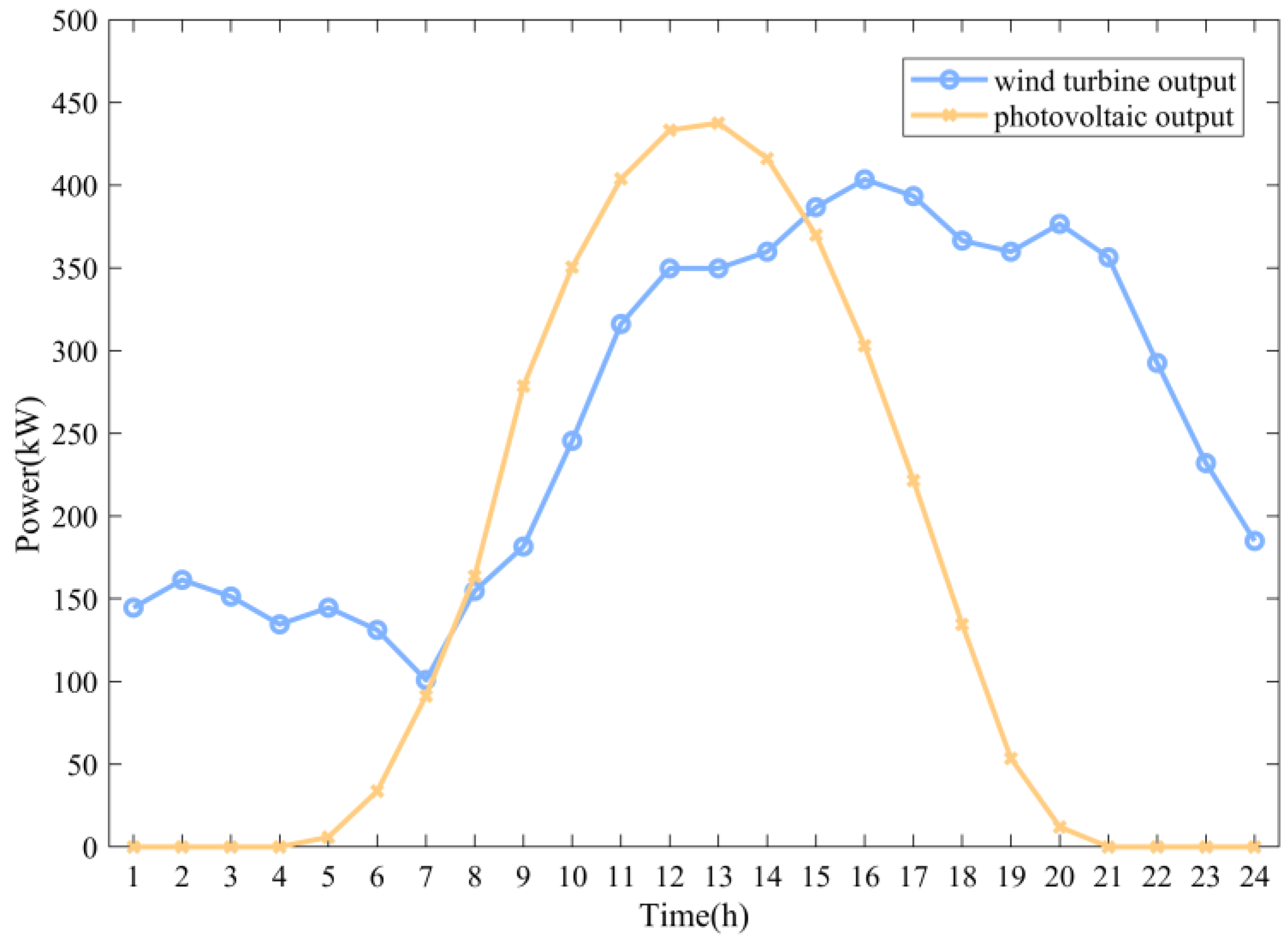
6.1. Experimental Data

This experiment first establishes a shared system model for the EVIES and the wind-solar-storage system for high-rise buildings. The core of the model lies in configuring the capacity of the PV system, WT system, and battery storage system (BESS) within the EVIES. Thus, the decision variables of the capacity configuration model include the installed capacities of the PV system, wind turbine system, and BESS. The decision variables of the optimization model involve the percentage of the number of batteries in the battery storage system at the beginning of each period with a fully charged state, the amount of SOC discharged by the EV, and the change in SOC of the energy storage battery of the high-rise building during each period. The MSCSO, based on a mutation-dominated selection strategy, is employed to validate the effectiveness of the model. The optimization model performs capacity allocation based on the known wind speed, light intensity, temperature, and load profiles and is tested under four different cases to maximize the daily economic return, minimize the load variance on the building’s grid side, and reduce overall carbon emissions.

Case 1:

No photovoltaic generation system in the EVIES vs. impacts under normal conditions

Case 2:

No wind turbine power generation system in the EVIES and the impact under normal conditions

Case 3:

High-rise building without the wind-solar hybrid system and its impact under normal conditions

Case 4:

Shared model of the EVIES and the building wind-solar-storage system designed under normal conditions

All tests are based on the same initialization parameters to ensure the validity of the experiments. Specifically, the population size is N = 200, the iteration limit is T = 800, and each algorithm is run independently 12 times. Since the data on PV output, wind turbine output, traffic flow, and other factors in the shared model of the EVIES and high-rise building system are small and negligible compared to the primary grid load, the shared model is integrated into the regional grid of the high-rise building. A typical daily load curve for a high-rise building is used in the simulation experiments, as shown in Figure 4 [34]. The outputs of the PV system and wind turbine in the EVIES model are calculated using light intensity, temperature, and wind speed data provided by Weatherbit (see Figure 5), as detailed in Section 3.1 and Section 3.2. Due to the height advantage, the top of a high-rise building typically experiences higher wind speeds and more intense light conditions than at ground level, thus improving the output performance of the wind-solar power generation system [35,36,37,38]. According to the vertical wind speed distribution, the wind speed at the top of the building is approximately 1.2 to 1.5 times that at ground level, depending on the building’s height and surrounding environment [39]. Additionally, light intensity remains relatively stable, but as the building height increases and shading effects diminish, it may increase slightly. Traffic flow data is obtained by surveying the number of EVs charged at multiple local charging stations at different time periods, and then scaled for experimental reference, as shown in Figure 6 [40]. The electricity pricing reference is based on a peak-valley time-of-use tariff strategy, as shown in Figure 7, and serves as the basis for the electricity pricing of the integrated charging station and building wind-solar-storage sharing model [41]. Equipment parameters of the EVIES and high-rise building wind-solar-storage sharing system as shown in

Table 3. Equipment parameters of the EVIES and high-rise building wind-solar-storage sharing system [42,43,44,45,46,47].

Parameter	Parameter Descriptions	Value
$\eta$.	Penalty Coefficient	5%
$r$	Depreciation Rate	10%
$Q_{ev}$	Electric Vehicle Battery Capacity	60
$y$	Service Life of WT/PV Panels	20
$C_{bess}$	Cost per Storage Unit	3.8 × 104
$C_{pv}$	Cost per Photovoltaic Unit	2.5 × 105
$C_{wt}$	Cost per Wind Turbine	4.0 × 105
${\alpha }_{PV}$	PV Operation and Maintenance Cost	350
${\alpha }_{WT}$	WT Operation and Maintenance Cost	400

. Parameter optimization of multi-objective optimization algorithms as shown in

Table 4. Parameter optimization of multi-objective optimization algorithms.

Parameter	Value
Population size	200
Iteration limit	800
WT capacity range	[0, 20]
PV capacity range	[0, 20]
BESS capacity range	[5, 35]
Gird configuration boundary	[−800, 800]

.

6.2. Model Solution Algorithm Comparison

To comprehensively evaluate the performance of the multi-objective optimization algorithm MSCSO proposed in this paper, this study compares it with several classical algorithms (RVEA [48], IBEA [49], MOPSO, PESA-II [50], and NSGA-III). The comparison is primarily based on three metrics: HV, the distribution metric Spread [51], and runtime. Values in bold represent the best performance under each metric when compared across different algorithms, thus providing a reference for algorithm selection in practical applications.

As shown in

Table 5. Comparison of the metric HV.

Algorithm	Best	Mean	Worst
RVEA	8.7119 × 10−2	7.5150 × 10−2	5.5996 × 10−2
IBEA	1.3131 × 10−1	8.6035 × 10−2	6.4770 × 10−2
MOPSO	1.4139 × 10−1	1.0032 × 10−1	6.7300 × 10−2
PESAII	1.8204 × 10−1	1.1071 × 10−1	7.6691 × 10−2
NSGAIII	1.4477 × 10−1	9.0994 × 10−2	7.3874 × 10−2
MSCSO	2.1749 × 10−1	1.3622 × 10−1	1.0153 × 10−1

,

Table 6. Comparison of the metric Spread.

Algorithm	Best	Mean	Worst
RVEA	4.2080 × 10−1	5.0864 × 10−1	6.8773 × 10−1
IBEA	5.7496 × 10−1	7.2864 × 10−1	8.4125 × 10−1
MOPSO	4.7153 × 10−1	6.6695 × 10−1	7.7536 × 10−1
PESAII	4.6206 × 10−1	6.0788 × 10−1	7.1299 × 10−1
NSGAIII	4.8062 × 10−1	5.9100 × 10−1	1.0572 × 100
MSCSO	4.3778 × 10−1	4.9216 × 10−1	5.8144 × 10−1

and

Table 7. Comparison of the metric Runtime.

Algorithm	Best	Mean	Worst
RVEA	6.6068 × 101	6.8773 × 101	7.2733 × 101
IBEA	7.6709 × 101	8.0941 × 101	8.9851 × 101
MOPSO	6.2577 × 101	6.3508 × 101	6.5675 × 101
PESAII	6.1712 × 101	6.6480 × 101	7.2818 × 101
NSGAIII	6.5148 × 101	6.6747 × 101	6.9045 × 101
MSCSO	5.8144 × 10−1	6.1741 × 101	6.2913 × 101

, in the comparison of multiple algorithms (e.g., RVEA, IBEA, MOPSO, PESA-II, and NSGA-III) and the MSCSO proposed in this paper for solving the model, MSCSO demonstrates excellent overall performance, especially in solving the EVIES and high-rise building wind-solar-storage sharing system model. Specifically, MSCSO shows significant improvements in two key metrics: hypervolume (HV) and Spread. The HV value of MSCSO is 1.3622 × 10⁻¹, an improvement of about 36.38% compared to the average HV value (6.8032 × 10⁻²) of all algorithms, highlighting its advantage in covering the Pareto front. Additionally, the Spread value of MSCSO is 4.9216 × 10⁻¹, which is about 18.10% lower than the average Spread value (5.8009 × 10⁻¹) of all algorithms, indicating better solution set uniformity and diversity. Moreover, the runtime of the MSCSO is 6.1741 × 10¹, which is approximately 2.73% lower than the average runtime (68.0317) of all algorithms, demonstrating a higher solving efficiency. Although MSCSO performs well in most tests, its results for the best Spread value do not reach the expected optimal level, suggesting that MSCSO may have some limitations in solution set uniformity in certain scenarios. Therefore, although the MSCSO has significant advantages over traditional multi-objective optimization algorithms, such as NSGA-III, PESA-II, MOPSO, and IBEA, its local search strategy requires further optimization to improve the uniformity and global coverage of the solution set.

Table 8. Comparison of objective function 1.

Algorithm	Functions1
	Min	Max
RVEA	−3655.6730	−3411.3412
IBEA	−4558.7595	−4350.4675
MOPSO	−4326.8892	−3604.3204
PESAII	−4463.7385	−3651.7192
NSGAIII	−4378.6923	−4293.6201
MSCSO	−4884.1325	−4533.8327

,

Table 9. Comparison of objective function 2.

Algorithm	Functions2
	Min	Max
RVEA	138,347.4705	147,149.2357
IBEA	136,205.4731	155,717.2408
MOPSO	157,058.4080	205,616.7163
PESAII	164,521.5865	181,832.5745
NSGAIII	139,623.6120	155,724.9789
MSCSO	134,676.4628	141,107.6105

and

Table 10. Comparison of objective function 3.

Algorithm	Functions3
	Min	Max
RVEA	833.4063	968.3241
IBEA	703.9207	1071.4816
MOPSO	606.8311	1131.7989
PESAII	563.0736	741.2197
NSGAIII	915.3269	1093.5630
MSCSO	580.6526	698.1306

present a comparison of the objective function values obtained using different algorithms during the solution process. For the two objectives of maximizing daily economic benefits and minimizing grid-side load fluctuations, MSCSO outperforms the other algorithms with a distinct advantage. Specifically, to maximize daily economic benefits, the maximum value of MSCSO is 14.08% higher than the average maximum value of all the algorithms, and the minimum value is 11.56% higher than the average minimum value. Furthermore, MSCSO also performs significantly better than the other algorithms in minimizing grid-side load fluctuations. Although the maximum value of MSCSO is, on average, 14.24% lower than the overall maximum, and the minimum value is, on average, 7.17% lower than the overall minimum, these results show that MSCSO converges to better solutions more quickly and that these solutions better meet practical application requirements.

However, MSCSO performs slightly worse in minimizing overall carbon emissions, especially when compared to the PESA-II algorithm. In particular, MSCSO shows a weaker performance in terms of the minimum value, indicating that its local optimization ability under carbon emission constraints needs further improvement. Specifically, the maximum value of MSCSO is, on average, 26.57% lower than the overall maximum, and the minimum value is, on average, 17.11% lower than the overall minimum. This suggests that, while MSCSO performs well overall in multi-objective optimization tasks, its multi-objective coordination and global search capabilities may require further enhancement to better address more complex optimization problems with stringent constraints.

6.3. Experimental Results Analysis

In this paper, we design a model for an integrated EVIES and high-rise building wind-solar-storage sharing system, which includes a battery storage system, photovoltaic system, and wind power generation system, creating an integrated solution for electric vehicle charging and building energy management. The MSCSO proposed in Chapter 5 is used to solve the model. When solving the system model configured under normal conditions, since only one reasonable and feasible solution is required, the ETOPSIS method [52] is employed to determine the installed capacity of the photovoltaic system, wind turbines, and battery storage system. The ETOPSIS method combines the entropy weight method and the TOPSIS method to objectively determine the weights of evaluation indexes, evaluate how close each solution is to the ideal solution, and perform a comprehensive evaluation of multiple indicators. After determining the optimal configuration using the ETOPSIS method, the optimized operation effects under four different scenarios are further analyzed, demonstrating the superiority of the system model designed under normal conditions across various performance metrics. For the design model under normal conditions (Case 4), the optimal installed capacity configuration is: 3 wind turbines, 14 photovoltaic units, and 29 batteries in the battery storage system. With this configuration, the model’s objective function achieves optimal solutions as follows: $F1=4703.17 CNY$, $F2=130956.28$, $F3=570.99 \mathrm{kg}$.

In Section 6.1, the analysis of the charging, discharging, and swapping quantities of the EVIES and the high-rise building wind-solar-storage sharing system throughout each time period leads to the following conclusions: The actual charging, discharging, and swapping quantities, calculated based on the initial battery storage system state and the charging and discharging demand for each period (as shown in Figure 8), It is evident that in most periods, the total number of charging, discharging, and swapping actions does not exceed the capacity of the available charging/discharging devices, and the total actions remain less than or equal to the number of EVs in circulation. This indicates that the system is able to meet the demands of EV users during the majority of periods. However, between 13:00–14:00 and 19:00–20:00, the total number of charging and discharging devices is insufficient relative to the total EV traffic flow, indicating that the charging demand during these two periods is not fully met. This phenomenon reflects a charging insufficiency issue during peak hours. Nonetheless, the EV-integrated charging station and the wind-solar-storage sharing system for high-rise buildings can meet the EV demand during other periods, thereby verifying the high efficiency and adaptability of the system configuration designed in this experiment for the majority of time periods.

By comparing the results in Figure 8 with those in Figure 9, the following conclusions are drawn: the sum of the actual number of EV charging and swapping actions equals the planned number, indicating that the system can reasonably allocate charging operations to EVs that have not undergone battery swapping based on demand. Furthermore, the observed number of EV swaps consistently does not exceed the planned swaps, the number of EVs charged is always equal to or greater than the planned charging, and the number of EVs discharged never surpasses the planned discharges. These results suggest that the system’s charging, discharging, and swapping arrangements during the experiment were reasonable and met expectations. For the 13:00–14:00 period, the planned number of EVs to be swapped was 6, the planned number of EVs to be charged was 4, and the planned number of EVs to be discharged was 4. The actual numbers were 0 swapped, eight charged, and four discharged. This variation reflects the system’s prioritization of EV charging demands during this period, which led to an inability to meet all swapping demands. This is in line with the system’s prioritization constraints: the charging demand is prioritized, and swapping demands are adjusted when resources are limited.

Further analysis reveals that, in all time periods, the actual number of battery swaps for electric vehicles is always less than or equal to the total count of fully charged batteries, indicating that the battery swapping operations of the EVIES and the high-rise building wind-solar-storage sharing system fully meet the capacity requirements. The number of swapped batteries does not exceed the capacity limit of the BESS. This further validates the reasonableness of the battery swapping operations in the design of the EVIES and wind-solar-storage sharing system, demonstrating that the system can effectively arrange swapping tasks based on the battery storage capacity, thus preventing excessive demand. During the time periods of 00:00–06:00, 12:00–15:00, and 20:00–24:00, the total count of fully charged batteries in the storage system is relatively low and does not exceed 50% of the charging capacity, indicating that the charging demand for electric vehicles during these periods is well met. The system’s charging arrangements are reasonable, ensuring the high efficiency of battery charging.

The SOC values at the beginning of each period for the BESS in the high-rise building are displayed in Figure 10, illustrating the charging and discharging patterns over a 24-h cycle. As depicted, the SOC begins at 0.2 at 00:00 and remains at 0.2 at 24:00, fulfilling the system’s initial and terminal equilibrium constraints. This shows that the BESS has effectively regulated its charging and discharging operations, avoiding both over-charging and deep discharging. Specifically, an increase in SOC reflects charging, indicating that the system is storing energy from external sources, such as the grid and renewable resources like photovoltaics and wind power. Conversely, a decrease in SOC indicates discharging to either meet the building’s energy demand or recharge electric vehicles.

During the 00:00–06:00 period, when the power demand is relatively low, the system remains in a charging state for most of the time, and the SOC remains stable. In the 06:00–09:00 period, despite being the morning peak time, the system still maintains relatively smooth SOC variations, indicating that it successfully manages the building’s lower power demand with moderate charging operations. During higher demand periods, such as the 12:00–15:00 noon hours, the SOC fluctuates significantly due to higher building loads, with the BESS discharging to meet the power demand while also performing some charging. In the 17:00–20:00 evening hours, as EV charging demand increases, the BESS discharges to either the EVs or the building, leading to more significant SOC fluctuations. Overall, the charging and discharging operations of the BESS over the 24-h period are dynamic and balanced, in line with the expected energy management strategy. This ensures stable operation under varying load conditions, while also ensuring the efficient utilization of the batteries and avoiding the risks of overcharging or over-discharging.

In the model, the energy flow relationship between the subsystems is shown in Figure 11. Based on actual data, the energy interaction process between the EVIES, the battery storage system, the power grid, and the high-rise building is analyzed, and the energy deployment of the system during load fluctuations is demonstrated. During the 00:00–06:00 period, when the power demand is relatively low, the system is in a charging state for most of the time, and the SOC of the BESS remains stable. Power is primarily supplied through a power grid or photovoltaic system to support the building’s electricity demand. Since the output of the photovoltaic system is low, the battery storage system provides power to both the building and the EVs, ensuring that the base load demand of the building is met. In the 06:00–09:00 period, during the morning peak hours, despite the gradual increase in power demand, the system maintains relatively smooth SOC variations, indicating that it effectively meets the power demand within the building by performing moderate charging operations of the battery storage system. During the 12:00–15:00 period, when the photovoltaic system generates a significant amount of power, the system mainly supplies power to the BESS and the high-rise building. As the demand for EV charging increases significantly during this period, the discharge of the BESS also increases, with supplementary power being drawn from the grid. This results in noticeable fluctuations in the charging and discharging processes. In the 17:00–20:00 evening period, as the demand for EV charging rises, both the BESS and the grid must collaborate to meet the power demands of the building and the EVs. During this period, the battery storage system may need to discharge more while also moderately charging to prepare for the subsequent peak load. The photovoltaic wind turbine system exhibits unidirectional energy flow to the subsystems, particularly during periods of strong photovoltaic generation, supplying power to the battery storage system and high-rise building. However, during the night, when the photovoltaic output decreases, the EVs and building rely more heavily on the battery storage system and grid to meet their power needs.

In the model, the load curve of the EVIES and the high-rise building wind-solar-storage sharing system after the grid connection is shown in Figure 12. The experimental results indicate that after the grid connection, the load fluctuation is significantly reduced, and the load curve becomes smoother. The maximum load after grid connection is 2201.52 kW, the minimum load is 997.00 kW, and the peak-to-valley difference is 1204.52 kW. In comparison, the original load curve has a maximum load of 2257 kW, a minimum load of 889 kW, and a peak-to-valley difference of 1368 kW. It can be observed that the fluctuation in load is effectively reduced after the system is connected to the grid, especially during peak periods (10:00–12:00) and afternoon periods (14:00–20:00). During these periods, the collaborative operation of the BESS and the grid effectively reduces the peak load on the grid, alleviates grid pressure, prevents excessive grid loading, and enhances load regulation stability. This demonstrates that the combination of photovoltaic wind energy and energy storage systems not only achieves peak shaving and valley filling but also significantly improves the system’s operational stability and reliability. Especially during low-demand periods (such as 00:00–07:00), the BESS reserves energy through charging, providing support for subsequent peak periods and further balancing the load. Through the optimized energy management strategy, the grid-connected operation of the EVIES and high-rise building wind-solar-storage sharing system has significantly improved in terms of load regulation, peak shaving, valley filling, and energy utilization efficiency, fully showcasing the system’s load allocation and energy management capabilities.

To further validate the rationality of the model, the settings for four different cases are evaluated after determining the optimal installed capacity configuration. The model settings for each case are listed in

Table 11. Model Settings for Different Cases.

CASE	EVIES-PV	EVIES-WT	Building-WT/PV
Case 1		√	√
Case 2	√		√
Case 3	√	√
Case 4	√	√	√

. The other constraints are consistent with the EVIES and high-rise building model developed in this chapter. The EWM-TOPSIS method is employed to determine the optimal operating scheme for each of the four cases. The comparison results of the model settings and their corresponding objective function values for each case are presented below.

As shown in Figure 13, the experimental results indicate that in terms of daily economic revenue, Case 4 generates higher revenue than Cases 1 and 2 but lower than Case 3 after the setup. The total profit in Case 4 increased by 26.54% compared to the average profit of the other scenarios. The daily economic revenue without the participation of the building’s wind-solar system is higher than that of the original design model. However, in terms of carbon emissions, it significantly exceeds the levels of both the original design model and the other comparison models, where the original design model exhibits the lowest carbon emissions, meeting the green carbon emission reduction requirements for sustainable development, as shown in Figure 14. Carbon emissions are reduced by 37.59% compared to the average emissions of the comparison models. In the case without the building’s wind system (Case 3), although the daily economic revenue increases compared to the original design model, carbon emissions rise substantially above both the original model and other comparison models. The configurations without photovoltaic (Case 1) or wind turbines (Case 2) significantly reduce the system’s energy self-sufficiency, leading to an increase in carbon emissions. This result demonstrates that the wind-photovoltaic system not only enhances the economic efficiency of the integrated energy station but also shows significant advantages in terms of carbon emissions and environmental friendliness.

As shown in Figure 15, the performance across the four cases shows significant differences in the peak-to-valley difference of the model’s grid-connected load. The load fluctuations in the original design model (Case 4) are more moderate compared to those in the other models, indicating that this scenario exhibits better stability in load regulation and peak-valley balancing. Specifically, Case 4 shows a peak load of 2189.00 kW, a valley load of 920.88 kW, and a peak-to-valley difference of 1268.12 kW, reflecting relatively stable grid load fluctuations. In contrast, Case 3 shows the largest peak-to-valley difference, with a peak load of 2625.47 kW, valley load of 691.46 kW, and peak-to-valley difference of 1934.01 kW. This indicates that in Case 3, the grid load fluctuates significantly, and there is a pronounced issue with load fluctuation. This is likely due to the lack of coordination with the wind-solar-storage sharing system of the EVIES, which reduces the power grid’s ability to regulate the load. In Case 2, the peak-to-valley difference is 1732.68 kW, with a peak load of 2340.74 kW and a valley load of 608.06 kW. Although the peak value is higher, the valley value is lower, and the peak-to-valley difference is reduced compared to Case 3. However, noticeable fluctuations remain, suggesting that the absence of wind power generation causes difficulties in load balancing. In Case 1, the peak-to-valley difference is 1730.01 kW, with a peak load of 2407.45 kW and a valley load of 677.44 kW. Although this scenario exhibits smaller load fluctuations compared to Case 3, the peak-to-valley difference remains high, primarily due to the absence of a photovoltaic power generation system, which reduces the system’s energy self-sufficiency and, consequently, affects the grid’s load stability. Therefore, Case 3 exhibits the largest peak load and the most significant fluctuations, while Case 2 has the lowest valley value but still experiences considerable fluctuations. In contrast, Case 4, the original design model, demonstrates the smallest peak-to-valley difference, indicating better reliability and stability in grid-connected operation, as well as more effective handling of grid-load variations.

Figure 16 illustrates the variation in the battery degradation rates for 200 optimized schemes under different cases. It can be observed that under normal conditions (Case 4), the battery degradation rate is the lowest, with a range between 0.00019% and 0.210%. This indicates that the battery health is well-maintained due to the integrated energy station and building wind-solar-storage shared model. In contrast, in Case 1 (no photovoltaic system) and Case 2 (no wind turbine system), the battery degradation rate increases significantly due to the lack of renewable energy system support, with degradation ranges of 0.00049% to 0.2918% and 0.00036% to 0.2694%, respectively. This suggests that without these energy systems, the battery bears a greater load, leading to increased degradation. Therefore, the proper configuration of photovoltaic and wind turbine systems is crucial for extending battery lifespan.

7. Conclusions

With the rapid advancement of renewable energy, the phenomenon of wind and light abandonment has become increasingly prominent, emphasizing the importance of rationally allocating renewable energy resources. In the shared system of the EVIES and high-rise building wind-solar-storage, optimizing the installed capacities of photovoltaic systems, wind turbines, and battery storage is critical for improving energy utilization efficiency and system stability. This study developed an optimization model for the EVIES and high-rise building wind-solar-storage sharing system, aiming to achieve energy complementarity and resource optimization through collaborative scheduling to meet the energy demands of all stakeholders. The optimization objectives include maximizing the daily economic return of the EVIES, minimizing the grid-side load variance of the building, and reducing the overall carbon emissions to balance the economic benefits and environmental sustainability. To address this complex multi-objective optimization problem, this paper proposes an MSCSO based on a mutation-dominated selection strategy, inspired by the SCSO and incorporating improvements such as positional mutation and dominance relationship judgment. The effectiveness of this improved algorithm in optimizing the wind-solar-storage sharing system for EVIES and high-rise buildings is verified through comparisons with other optimization algorithms. The experimental results show that after the grid connection, the system load curve is smoothed, significantly reducing the peak-to-valley difference and enhancing the overall operational stability. Compared to the design experimental model, the optimized system increases the daily economic return by an average of 26.54% and reduces carbon emissions by 37.59%. These results validate the reasonableness of the model configuration optimization and demonstrate the proposed optimization algorithm’s potential to enhance both the economic and environmental performance of the system. Therefore, this study provides theoretical support for the configuration optimization of EVIES and high-rise building wind-solar-storage sharing systems, while offering new insights and methodologies for the sustainable development of green, low-carbon energy systems.

References

1. Lu, Q.; Liu, M. A multi-criteria compromise ranking decision-making approach for analysis and evaluation of community-integrated energy service system. Energy 2024, 306, 132439. [Google Scholar] [CrossRef]
2. Talihati, B.; Tao, S.; Fu, S.; Zhang, B.; Fan, H.; Li, Q.; Lv, X.; Sun, Y.; Wang, Y. Energy storage sharing in residential communities with controllable loads for enhanced operational efficiency and profitability. Appl. Energy 2024, 373, 123880. [Google Scholar] [CrossRef]
3. Sun, B. A multi-objective optimization model for fast electric vehicle charging stations with wind, PV power and energy storage. J. Clean. Prod. 2021, 288, 125564. [Google Scholar] [CrossRef]
4. Liao, X.; Qian, B.; Jiang, Z.; Fu, B.; He, H. Integrated Energy Station Optimal Dispatching Using a Novel Many-Objective Optimization Algorithm Based on Multiple Update Strategies. Energies 2023, 16, 5126. [Google Scholar] [CrossRef]
5. Shen, H.; Zhang, H.; Xu, Y.; Chen, H.; Zhu, Y.; Zhang, Z.; Li, W. Multi-objective capacity configuration optimization of an integrated energy system considering economy and environment with harvest heat. Energy Convers. Manag. 2022, 269, 116116. [Google Scholar] [CrossRef]
6. Zhang, S.; Li, X.; Li, Y.; Zheng, Y.; Liu, J. A green-fitting dispatching model of station cluster for battery swapping under charging-discharging mode. Energy 2023, 276, 127600. [Google Scholar] [CrossRef]
7. Yang, J.; Liu, W.; Ma, K.; Yue, Z.; Zhu, A.; Guo, S. An optimal battery allocation model for battery swapping station of electric vehicles. Energy 2023, 272, 127109. [Google Scholar] [CrossRef]
8. Linjuan, Z.; Han, F.; Zhiheng, Z.; Shangbing, W.; Jinbin, Z. Site selection and capacity determination of charging stations considering the uncertainty of users’ dynamic charging demands. Front. Energy Res. 2024, 11, 1295043. [Google Scholar] [CrossRef]
9. Ang, Y.Q.; Polly, A.; Kulkarni, A.; Chambi, G.B.; Hernandez, M.; Haji, M.N. Multi-objective optimization of hybrid renewable energy systems with urban building energy modeling for a prototypical coastal community. Renew. Energy 2022, 201, 72–84. [Google Scholar]
10. Çiçek, A. Multi-Objective Operation Strategy for a Community with RESs, Fuel Cell EVs and Hydrogen Energy System Considering Demand Response. Sustain. Energy Technol. 2023, 55, 102957. [Google Scholar] [CrossRef]
11. Ge, J.; Shen, C.; Zhao, K.; Lv, G. Energy production features of rooftop hybrid photovoltaic–wind system and matching analysis with building energy use. Energy Convers. Manag. 2022, 258, 115485. [Google Scholar] [CrossRef]
12. Xie, Y.; Li, J.; Li, Y.; Zhu, W.; Dai, C. Two-stage evolutionary algorithm with fuzzy preference indicator for multimodal multi-objective optimization. Swarm Evol. Comput. 2024, 85, 101480. [Google Scholar]
13. Shen, J.; Wang, P.; Dong, H.; Wang, W.; Li, J. Surrogate-assisted evolutionary algorithm with decomposition-based local learning for high-dimensional multi-objective optimization. Expert Syst. Appl. 2024, 240, 122575. [Google Scholar] [CrossRef]
14. Hadikhani, P.; Lai, D.T.C.; Ong, W.H. Human Activity Discovery with Automatic Multi-Objective Particle Swarm Optimization Clustering with Gaussian Mutation and Game Theory. IEEE Trans. Multimed. 2024, 26, 420–435. [Google Scholar] [CrossRef]
15. Yang, W.; Liu, S.; Yang, J. An optimized surrogate model and algorithm with rapid multi-parameter processing capability for antenna design. Measurement 2025, 241, 115719. [Google Scholar]
16. Wei, L.; Li, E. A Grey Prediction-Based Reproduction Strategy for Many-Objective Evolutionary Algorithm. Int. J. Intell. Syst. 2024, 2024, 8994938. [Google Scholar]
17. Gao, X.; Song, S. A switching competitive swarm optimizer for multi-objective optimization with irregular Pareto fronts. Expert Syst. Appl. 2024, 255, 124641. [Google Scholar]
18. Jameel, M.; Abouhawwash, M. Multi-objective Mantis Search Algorithm (MOMSA): A novel approach for engineering design problems and validation. Comput. Methods Appl. Mech. Eng. 2024, 422, 116840. [Google Scholar]
19. Seyyedabbasi, A.; Kiani, F. Sand Cat swarm optimization: A nature-inspired algorithm to solve global optimization problems. Eng. Comput. 2023, 39, 2627–2651. [Google Scholar] [CrossRef]
20. Jia, J.; Li, H.; Wu, D.; Guo, J.; Jiang, L.; Fan, Z. Multi-objective optimization study of regional integrated energy systems coupled with renewable energy, energy storage, and inter-station energy sharing. Renew. Energy 2024, 225, 120328. [Google Scholar]
21. Zhang, X.; Gao, W.; Zhong, J. Decentralized Economic Dispatching of Multi-Micro Grid Considering Wind Power and Photovoltaic Output Uncertainty. IEEE Access 2021, 9, 104093–104103. [Google Scholar] [CrossRef]
22. Zhu, Y.; Yang, S.; Ge, B.; Li, Y. Design optimization and uncertainty analysis of multi-energy complementary system for residential building in isolated area. Energy Convers. Manag. 2021, 241, 114310. [Google Scholar]
23. Deltenre, Q.; De Troyer, T.; Runacres, M.C. Performance assessment of hybrid PV-wind systems on high-rise rooftops in the Brussels-Capital Region. Energy Build. 2020, 224, 110137. [Google Scholar]
24. Asdrubali, F.; Baldinelli, G.; Scrucca, F.; D Alessandro, F. Life Cycle Assessment of electricity production from renewable energies: Review and results harmonization. Renew. Sustain. Energy Rev. 2015, 42, 1113–1122. [Google Scholar]
25. Coello, C.A.; Lechuga, M.S. MOPSO: A proposal for multiple objective particle swarm optimization. In Proceedings of the 2002 Congress on Evolutionary Computation, CEC’02 (Cat. No.02TH8600), Honolulu, HI, USA, 12–17 May 2002; pp. 1051–1056. [Google Scholar]
26. Nebro, A.J.; Durillo, J.J.; Luna, F.; Dorronsoro, B.; Alba, E. MOCell: A cellular genetic algorithm for multiobjective optimization. Int. J. Intell. Syst. 2009, 24, 726–746. [Google Scholar]
27. Vu, C.C.; Bui, L.T.; Abbass, H.A. DEAL: A Direction-Guided Evolutionary Algorithm; Bui, L.T., Ong, Y.S., Hoai, N.X., Ishibuchi, H., Suganthan, P.N., Eds.; Springer: Berlin/Heidelberg, Germany, 2012; pp. 148–157. [Google Scholar]
28. Deb, K.; Jain, H. An Evolutionary Many-Objective Optimization Algorithm Using Reference-Point-Based Nondominated Sorting Approach, Part I: Solving Problems with Box Constraints. IEEE Trans. Evol. Comput. 2014, 18, 577–601. [Google Scholar]
29. Deb, K.; Thiele, L.; Laumanns, M.; Zitzler, E. Scalable Test Problems for Evolutionary Multiobjective Optimization. In Evolutionary Multiobjective Optimization: Theoretical Advances and Applications; Abraham, A., Jain, L., Goldberg, R., Eds.; Springer: London, UK, 2005; pp. 105–145. [Google Scholar]
30. Deb, K.; Thiele, L.; Laumanns, M.; Zitzler, E. Scalable multi-objective optimization test problems. In Proceedings of the 2002 Congress on Evolutionary Computation, CEC’02 (Cat. No.02TH8600), Honolulu, HI, USA, 12–17 May 2002; pp. 825–830. [Google Scholar]
31. van Veldhuizen, D.A. Evolutionary Computation and Convergence to a Pareto Front. In Late Breaking Papers at the Genetic Programming 1998 Conference; Stanford University Bookstore: Stanford, CA, USA, 1998. [Google Scholar]
32. Coello, C.A.C.; Cortés, N.C. Solving Multiobjective Optimization Problems Using an Artificial Immune System. Genet. Program. Evolvable Mach. 2005, 6, 163–190. [Google Scholar]
33. Zitzler, E.; Thiele, L. Multiobjective evolutionary algorithms: A comparative case study and the strength Pareto approach. IEEE Trans. Evol. Comput. 1999, 3, 257–271. [Google Scholar]
34. Liao, X.; Ma, J.; Jiang, Z.; Zhou, J. Many-objective optimization based mutual feed scheduling for energy system of integrated energy station. Appl. Soft Comput. 2024, 161, 111803. [Google Scholar]
35. Häder, D.; Cabrol, N.A. Monitoring of Solar Irradiance in the High Andes. Photochem. Photobiol. 2020, 96, 1133–1139. [Google Scholar]
36. Li, Q.S.; Shu, Z.R.; Chen, F.B. Performance assessment of tall building-integrated wind turbines for power generation. Appl. Energy 2016, 165, 777–788. [Google Scholar] [CrossRef]
37. Fagiano, L.; Milanese, M.; Piga, D. High-Altitude Wind Power Generation. IEEE Trans. Energy Convers. 2010, 25, 168–180. [Google Scholar] [CrossRef]
38. Blumthaler, M.; Ambach, W.; Ellinger, R. Increase in solar UV radiation with altitude. J. Photochem. Photobiol. B Biol. 1997, 39, 130–134. [Google Scholar] [CrossRef]
39. Murakami, S.; Uehara, K.; Komine, H. Amplification of wind speed at ground level due to construction of high-rise building in urban area. J. Wind Eng. Ind. Aerodyn. 1979, 4, 343–370. [Google Scholar] [CrossRef]
40. Quddus, M.A.; Shahvari, O.; Marufuzzaman, M.; Usher, J.M.; Jaradat, R. A collaborative energy sharing optimization model among electric vehicle charging stations, commercial buildings, and power grid. Appl. Energy 2018, 229, 841–857. [Google Scholar] [CrossRef]
41. Wang, R.; Mu, J.; Sun, Z.W.; Wang, J.; Hu, A. NSGA-II multi-objective optimization regional electricity price model for electric vehicle charging based on travel law. Energy Rep. 2021, 7, 1495–1503. [Google Scholar] [CrossRef]
42. Roslan, M.F.; Ramachandaramurthy, V.K.; Mansor, M.; Mokhzani, A.S.; Jern, K.P.; Begum, R.A.; Hannan, M.A. Techno-economic impact analysis for renewable energy-based hydrogen storage integrated grid electric vehicle charging stations in different potential locations of Malaysia. Energy Strategy Rev. 2024, 54, 101478. [Google Scholar] [CrossRef]
43. Abid, M.S.; Ahshan, R.; Al Abri, R.; Al-Badi, A.; Albadi, M. Techno-economic and environmental assessment of renewable energy sources, virtual synchronous generators, and electric vehicle charging stations in microgrids. Appl. Energy 2024, 353, 122028. [Google Scholar] [CrossRef]
44. Khan, S.; Sudhakar, K.; Bin Yusof, M.H. Building integrated photovoltaics powered electric vehicle charging with energy storage for residential building: Design, simulation, and assessment. J. Energy Storage 2023, 63, 107050. [Google Scholar] [CrossRef]
45. Salek, F.; Resalati, S.; Morrey, D.; Henshall, P.; Azizi, A. Technical Energy Assessment and Sizing of a Second Life Battery Energy Storage System for a Residential Building Equipped with EV Charging Station. Appl. Sci. 2022, 12, 11103. [Google Scholar] [CrossRef]
46. Liu, G.; Xue, Y.; Chinthavali, M.S.; Tomsovic, K. Optimal Sizing of PV and Energy Storage in an Electric Vehicle Extreme Fast Charging Station. In Proceedings of the 2020 IEEE Power & Energy Society Innovative Smart Grid Technologies Conference (ISGT), Washington, DC, USA, 17–20 February 2020; pp. 1–5. [Google Scholar]
47. Mazzeo, D. Solar and wind assisted heat pump to meet the building air conditioning and electric energy demand in the presence of an electric vehicle charging station and battery storage. J. Clean. Prod. 2019, 213, 1228–1250. [Google Scholar] [CrossRef]
48. Cheng, R.; Jin, Y.; Olhofer, M.; Sendhoff, B. A Reference Vector Guided Evolutionary Algorithm for Many-Objective Optimization. IEEE Trans. Evol. Comput. 2016, 20, 773–791. [Google Scholar]
49. Yuan, J.; Liu, H.L.; Ong, Y.S.; He, Z. Indicator-Based Evolutionary Algorithm for Solving Constrained Multiobjective Optimization Problems. IEEE Trans. Evol. Comput. 2022, 26, 379–391. [Google Scholar]
50. Corne, D.W.; Knowles, J.D.; Oates, M.J. The Pareto Envelope-Based Selection Algorithm for Multiobjective Optimization; Schoenauer, M., Deb, K., Rudolph, G., Yao, X., Lutton, E., Merelo, J.J., Schwefel, H., Eds.; Springer: Berlin/Heidelberg, Germany, 2000; pp. 839–848. [Google Scholar]
51. Li, M.; Zheng, J. Spread Assessment for Evolutionary Multi-Objective Optimization; Ehrgott, M., Fonseca, C.M., Gandibleux, X., Hao, J., Sevaux, M., Eds.; Springer: Berlin/Heidelberg, Germany, 2009; pp. 216–230. [Google Scholar]
52. Huang, W.; Shuai, B.; Sun, Y.; Wang, Y.; Antwi, E. Using entropy-TOPSIS method to evaluate urban rail transit system operation performance: The China case. Transp. Res. Part A Policy Pract. 2018, 111, 292–303. [Google Scholar]
Figure 1. Structure diagram of the EVIES and high-rise building wind-solar-storage sharing system.
Sustainability 17 03142 g001
Figure 2. Energy flow and scheduling priorities in EVIES and high-rise building wind-solar-storage system.
Sustainability 17 03142 g002
Figure 3. Flowchart of MSCSO algorithm.
Sustainability 17 03142 g003
Figure 4. Daily load data curves for high-rise buildings.
Sustainability 17 03142 g004
Figure 5. Wind and PV output curves.
Sustainability 17 03142 g005
Figure 6. Electric vehicle swapping/charging/discharging quantity.
Sustainability 17 03142 g006
Figure 7. Peak-valley time-of-use electricity price and electricity price for sale and purchase.
Sustainability 17 03142 g007
Figure 8. Actual number of electric vehicle charging, discharging, and swapping operations.
Sustainability 17 03142 g008
Figure 9. Number of batteries in the full and empty states of the EVIES energy storage system.
Sustainability 17 03142 g009
Figure 10. SOC changes in the battery storage system of the high−rise building.
Sustainability 17 03142 g010
Figure 11. Energy flow diagram between subsystems of the shared system model.
Sustainability 17 03142 g011
Figure 12. Load curve after grid connection of the shared system model.
Sustainability 17 03142 g012
Figure 13. Hourly revenue and 24−h cumulative revenue for different cases.
Sustainability 17 03142 g013
Figure 14. Hourly carbon emissions and 24−h cumulative emissions for different cases.
Sustainability 17 03142 g014
Figure 15. Comparison of the 24−h grid−connected peak−valley load curves for different cases.
Sustainability 17 03142 g015
Figure 16. Battery loss rates of different schemes after optimization across various cases.
Sustainability 17 03142 g016