Abstract
Air quality is an essential factor for human health and ecosystem balance, but in regions like Petroșani Mountain Depression, air pollution continues to be a significant challenge. This area, marked by decades of coal mining, is confronted with high concentrations of pollutants, influenced by human activities and the specific geography and climate. This study aims to compare instrumental air quality measurements with snow sample analysis, as a sustainable alternative method. Specifically, it examines the spatiotemporal distribution and evolution of air pollutants, utilizing long-term monitoring data and an extensive sampling network (42 points) for both air and snow, to provide a thorough understanding of air quality dynamics in the area. The experimental part of this study focused on determining VOCs and PM in the air, and dissolved ions (sulfate, calcium, and magnesium) and suspended solids in snow. The results highlight significant correlations between pollution sources and atmospheric dynamics in mountain depressions, while also analyzing the efficiency of the instruments used for data collection. This study emphasizes that, although instrumental methods provide precise and detailed measurements, their implementation in isolated regions presents significant challenges. Therefore, alternative approaches such as snow analysis can represent a more efficient and sustainable option in these regions.
1. Introduction
Air pollution is a multifaceted issue characterized by the presence of various pollutants that influence both environmental quality and public health. Its impact is determined by concentration levels and exposure duration, with adverse effects arising either from acute exposure to high concentrations or prolonged exposure to lower levels.
In recent years, it has become a critical environmental challenge of global significance, often surpassing established national standards. Beyond its detrimental effects on human well-being and ecosystems, air pollution also plays a key role in driving climate change [1,2,3,4,5,6].
Despite significant advancements in air quality control, global mortality and loss of healthy life years due to air pollution have shown minimal reduction since the 1990s. Air pollution remains the second leading cause of death among non-contagious health reasons [3,7,8,9,10,11].
Air pollution can be classified as internal or external air pollution, depending on where the activities take place [3,12]. Outdoor air pollution occurs in an open environment, covering the entire atmosphere. The external air pollutants are mainly composed of nitrogen oxides (NOx), nitrogen dioxide (NO2), sulfur dioxide (SO2), ozone (O3), carbon monoxide (CO), hydrocarbons, and particulate matter (PM) of different particle sizes [3].
Particulate matter (PM), a complex mixture of solid and liquid particles of organic and inorganic substances suspended in the air, is considered the most common pollutant. Air pollution from PM (PM2.5 and PM10) poses a significant health threat to people living in cities. The health-damaging PM, which can penetrate deep into the lungs, contributes to the risk of developing cardiovascular diseases as well as lung cancer [3,13,14,15,16]. In addition to health problems affecting the low IAQ nervous system, its effects are associated with other long-term diseases [3,17]. Furthermore, PM2.5 affects the climate through both direct and indirect climatic impacts [18]. PM2.5 concentrations can be significantly reduced through CO2 emission reduction activities [19,20]. CO2 not only affects climate change, but also raises health-related issues [13].
Growing urban areas have the most diverse human activities; industrial processes and vehicular traffic mainly cause higher concentrations of pollutants [21,22,23,24].
Pollution by various elements is all around us, in aerosols, in snow, and in our rivers and oceans. Solutions are needed to the problems caused by the presence of air pollutants such as urban dust, SOx, NOx, CO, heavy metals, and chemical carcinogens in aerosols [25,26,27,28].
To assess and control pollution levels, researchers and authorities employ a range of advanced instrumental methods that enable precise measurement of atmospheric pollutant concentrations [29,30].
One of the most widely used methods is absorption and emission spectrometry, which includes UV–Vis spectrometry for measuring sulfur dioxide (SO2) and ozone (O3). Additionally, atomic absorption spectrometry (AAS) is employed for detecting heavy metals such as lead (Pb), cadmium (Cd), and mercury (Hg), while fluorescence spectrometry is effective for analyzing SO2 concentrations [31,32].
Another essential technique is gas chromatography (GC), which is used to identify volatile organic compounds (VOCs), polycyclic aromatic hydrocarbons (PAHs), and nitrogen oxides (NOx). This method is often combined with mass spectrometry (GC-MS) for a detailed analysis of harmful airborne substances [33,34].
At the same time, electrochemical sensors are used in monitoring stations and portable devices to detect gases such as carbon monoxide (CO), nitrogen dioxide (NO2), and sulfur dioxide (SO2). These devices are valued for their low cost and rapid response time [35].
For remote measurements, advanced technologies such as LiDAR (Light Detection and Ranging) enable the mapping of atmospheric pollutants using laser beams. Additionally, optical diffusion sensors are employed for monitoring suspended particles (PM10, PM2.5), contributing to a better understanding of their distribution in the air [5].
The gravimetric method is one of the most accurate techniques used for collecting and analyzing PM10 and PM2.5 on specialized filters. These filters are then examined to determine the chemical composition and sources of pollution [36,37].
For greenhouse gas monitoring, non-dispersive infrared (NDIR) analyzers are used to detect carbon dioxide (CO2). Additionally, tunable diode laser absorption spectroscopy (TDLAS) enables the detection of trace amounts of pollutants such as methane (CH4) and ammonia (NH3) [38,39].
These technologies are integrated into stationary air monitoring stations, mobile laboratories, and even Internet of Things (IoT) networks for real-time air quality analysis. The collected data provide a solid foundation for more effective environmental policies, contributing to improved air quality and the protection of public health [40].
The present paper addresses a timely issue related to the complex mechanisms that come into play after the restructuring of the Jiu Valley Mining Basin, with a particular focus on air quality in the Municipality of Petroșani, which has historically faced significant pollution issues due to bituminous coal extraction and processing. This study aims to compare instrumental air quality measurements with snow sample analysis. Specifically, it examines the spatiotemporal distribution and evolution of air pollutants, utilizing long-term monitoring data and an extensive sampling network for both air quality and snow samples, to provide a thorough understanding of air quality dynamics in the Petroșani Mountain Depression.
Despite the high precision and sensitivity offered by instrumental methods for air quality analysis, their application in mountainous regions faces multiple challenges. While essential for detailed measurements, these methods are often hindered by economic, technical, and accessibility-related factors. One major obstacle is the high cost of the equipment used. Devices such as mass spectrometers and gas analyzers require significant investments, not only for acquisition but also for maintenance. The harsh climatic conditions characteristic of mountainous areas accelerate equipment wear and tear, necessitating frequent repairs and calibrations. In addition to costs, the installation and accessibility of equipment present another significant challenge. Due to their size and weight, transporting these instruments across rugged terrain is difficult and requires additional logistical resources. Furthermore, inadequate infrastructure in such regions complicates the use of advanced equipment, as stable power sources and reliable data transmission connections are necessary. Maintenance and calibration interventions are also hindered by the difficulty of specialists accessing these remote locations. Another factor affecting the reliability of instrumental methods is their sensitivity to meteorological conditions. Extreme temperatures, high humidity, precipitation, and strong winds can impair sensor functionality, leading to measurement errors or even equipment failure. Additionally, atmospheric pressure variations may influence the analysis of pollutant concentrations, affecting the accuracy of the collected data. Frequent sensor calibration is essential for maintaining measurement accuracy. However, in mountainous areas with highly variable environmental conditions, implementing uniform calibration protocols is challenging. This lack of standardization can lead to discrepancies between measurements taken at different times or locations. Data collection and transmission also pose major obstacles due to the limited availability of telecommunications signals in remote areas. Equipment that relies on continuous internet connectivity for real-time data transmission may become ineffective in such environments. Moreover, the dependence on a stable power supply further complicates the use of these methods, as powering equipment in mountainous regions can be problematic. Beyond these limitations, external interferences and sample contamination can influence the results obtained. The presence of dust particles, ice, or other impurities can affect sensor accuracy. Finally, the limitations of specific methods must be considered. Optical and spectroscopic analyzers, for instance, struggle under low-visibility conditions (fog, low clouds), while electrochemical sensors have a short lifespan and degrade quickly in extreme environments. Moreover, methods requiring sample collection for laboratory analysis involve additional logistical challenges and do not provide real-time results, reducing their effectiveness in continuous air quality monitoring. Although instrumental methods are essential for precise air quality monitoring, their use in mountainous regions is constrained by numerous factors, including high costs, logistical difficulties, and sensitivity to environmental conditions [21,41,42,43]. In this context, a more flexible approach is needed—one that integrates hybrid technologies, combining low-cost sensors with advanced techniques and predictive models for more efficient monitoring.
An additional research and application direction in mountainous environmental monitoring is the analysis of snow quality as an indicator of atmospheric pollution. Snow can capture and accumulate airborne particles and pollutants, providing valuable insights into atmospheric composition over an extended period. Integrating air quality measurements with the chemical composition analysis of snow could offer crucial data on the impact of pollutants on mountain ecosystems and enhance pollution dispersion forecasting models in these remote regions. Thus, the implementation of complementary methods, incorporating both air analysis and the study of atmospheric deposits in the form of solid precipitation, could contribute to a deeper understanding of pollutant dynamics in mountainous areas.
Mountain depressions are unique ecological environments that, due to their specific topography and atmospheric dynamics, often exhibit distinct air quality characteristics [22,44]. These regions, which are naturally prone to temperature inversions and limited air circulation, can become hotspots for atmospheric pollution accumulation, impacting both the environment and human health. In light of these challenges, the municipality of Petroșani and its surrounding tourist areas, including the Rusu Zone and Parâng Resort, present an ideal setting for comprehensive pollution assessment studies [4,10,45].
Pollutants effectively accumulate in the snow, which acts as an aerodynamic mechanical barrier for particles that are suspended in the air. In comparison with soil, snow-cap functions only as a mechanical barrier for airborne pollutants, while soil is not only a mechanical barrier but also biogeochemical. Pollutants in the soil migrate horizontally and vertically [46,47,48,49,50].
Concentrations of chemical element soluble forms in snow-cap in urban and industrial areas are many times lower in comparison with insoluble ones (snow-dust), there-fore, a snowmelt water analysis is not always performed. However, there is a relationship between concentrations of soluble and insoluble particles. This relationship is characterized by inverse proportionality; that is, closer to pollution sources in urban and industrial areas, the proportion of soluble forms of metals decreases relatively, while the load of dust increases approaching the contaminated area. Generally, the ratio in the snow-cap of soluble and insoluble forms depends on the type of pollution source, the distance from the pollution source, and the load of snow-dust [48,51].
2. Materials and Methods
2.1. Overview of the Study Area
The Jiu Valley has a rich historical background, shaped by the presence of a fundamental natural resource—bituminous coal. The exploitation of coal, coupled with the Industrial Revolution, rapidly transformed a landscape traditionally characterized by pastoral and agrarian values into a major industrial center, deeply integrated and primarily focused on mining. The advancement of organizational and technological structures led to significant demographic growth, which, over time, necessitated the expansion of the built environment alongside the existing physical space, gradually acquiring the attributes of modernity [4,52]. The municipality of Petroșani, the administrative center of the Jiu Valley, is located in the homonymous depression, on the Eastern Jiu River, in the central, south-western part of Romania, in Hunedoara County, and covers an area of about 43.5 km² (Figure 1). The relief in the administrative territory is very uneven, specific to the mountainous area, with gorges on the routes of the two Jiu rivers (Eastern Jiu and West Jiu), the elevation of the land in the central area of the city being 600 m [4,52,53].

Figure 1.
The map of the studied area and the geomorphological representation of Petroșani Municipality and surroundings [54,55,56].
The elongated shape of the region, coupled with its encirclement by high mountains, gives rise to distinct climatic characteristics within the depression (Figure 2), with the city of Petroșani being no exception. Mountain ranges typically block the movement of air masses, and the shelter they provide inhibits the “ventilation” of the depression [4]. As a result, air masses circulate from north to south through the “windows” that separate the mountain ranges of Bănita–Merișor and Surduc–Lainici. Another notable thermal phenomenon in Petroșani is thermal inversion [1,52]. During winter, cloud layers descend into the low-lying depression areas, establishing a normal temperature gradient at 800 m altitude from the cloud base, which promotes the formation of an inverse temperature layer. This phenomenon further complicates the dispersion of atmospheric pollutants, as they remain longer in the polluted areas.

Figure 2.
Different stages of thermal inversion in the Petroșani Mountain Depression.
Located in the Parâng Mountains at an altitude of approximately 1800 m, not far from the municipality of Petroșani, Parâng Resort constitutes the main tourist area in the eastern part of the Jiu Valley [57]. It has a remarkably high tourism potential that, however, has not yet been fully exploited. Certified in 2009 as a national interest tourist resort, Parâng Resort has become increasingly known in recent years, especially among winter sports enthusiasts, due to its ski slopes and, more importantly, its relatively easy access. Although it does not have a rigorous urban planning system, the resort is equipped with numerous holiday homes, several tourist cabins, and facilities for educational purposes (such as the Sports Club School Petroșani cabin and the “Prof. Univ. Virgil Teodorescu” Teaching Base of the National University of Physical Education and Sport in Bucharest), as well as infrastructure for winter sports activities (ski lifts, chairlifts, rental centers, etc.). Access to the resort is made from the municipality of Petroșani, along county road DJ709 F to the Rusu area, over a distance of approximately 8–9 km. From here, access to the actual resort in the alpine Parâng area can be made as follows:
- By the old chairlift, commissioned in 1973, with a length of 2.24 km, a vertical rise of 612 m, and a speed of 2 m/s. It is the second longest chairlift in the country, after the one in Borșa, with the departure station located about 8 km from the city.
- By the new chairlift, TS3, put into operation in 2014, with the departure station located about 9 km from the city, in the Rusu area. This chairlift has a length of 2.2 km, a vertical rise of 420 m, and a speed of 6 m/s.
- By car, following the recent modernization of the terminal section of approximately 4.5 km of County Road 709 F, which connects the Rusu area to the alpine zone of Parâng Resort. Car access is only possible in summer, as this final segment is closed to public traffic in winter [58].
The workers’ colony (hereinafter referred to as the Historic quarter) in Petroșani emerged in the mid-19th century, during the Austro-Hungarian Empire, alongside the development of the mining industry. A characteristic of the neighborhood was its wide streets, which were unusually straight for that time.
The homes owned by miners at the end of the 19th century were of better quality than many of the bourgeois houses in other areas of Romania. Additionally, miners received vouchers for the purchase of coal, which they would then burn in their own heating systems in the homes within the workers’ colony. Those living in other neighborhoods connected to the centralized heating system could pay 50% of the costs for the Paroșeni district heating, which was extremely convenient for the population.
The coal-based heating systems in homes and district heating installations operate differently but produce the same essential energy sources for human use. The Paroșeni power plant produced electricity, thermal energy, and supplied hot water to the population. In the city’s historic areas (such as the Historic quarter, Livezeni, etc.), the centralized heating system was not implemented, and there is no natural gas supply network. As a result, the population continues to heat their homes in the traditional way during the cold season by burning various combustible materials (coal, textile, and footwear waste from the second-hand industry, etc.), which generates thermal energy. The smoke resulting from combustion is directly vented through the chimney, without any protective systems, filters, or pollutant retention mechanisms, releasing pollutants directly into the atmosphere. This represents a significant source of air pollution [59].
2.2. Sampling Site Layout
Air quality monitoring has been carried out using a combination of indirect (snow analysis) and direct (instrumental methods), over multiple stages and in distinct areas of Petroșani Municipality and its surroundings, as follows:
- The Rusu area and the Parâng resort;
- The central-northern part of the municipality, including the Brădet area;
- The workers’ colony/Historic quarter;
- The ring road.
In the Rusu/Parâng area, 11 air quality monitoring points were set, numbered from 1 to 11. The measurements were taken in a single session, during the winter, to capture any potential interference from pollution resulting from the heating of holiday homes/cabins in the area.
Consequently, being the most polluted neighborhood in the municipality of Petroșani, the Historic quarter has the highest number of air quality monitoring points, totaling 26. These were numbered from 12 to 37, and the measurements were taken during the winter, both at night and during the day, to capture fluctuations in the concentration of pollutants or particulate matters when the population was using heating sources, and when they were not required. Additional measurements were made in the central-northern part of the city, where there is direct exposure to the historic area, to assess any negative impact on air quality due to emissions from the houses in the former workers’ colony. Measurements were also taken in the Brădet area, located at a higher altitude than the city’s main area, where several villas are increasingly immersed in nature. A total of five monitoring points were placed there, numbered from 38 to 42. These measurements were also conducted during the winter, both at night and during the day, for the reasons mentioned above.
Subsequently, one more set of measurements was carried out in the winter of 2023 (February 14) to compare the values and assess the contribution of pollutants and suspended particles from household activities in the Historic quarter during the cold season. For this purpose, an additional monitoring point, P7, was introduced, located at the most polluted spot of the Historic quarter. By extending the monitoring and correlating the determined values with the timing of the measurements, seasonal, diurnal, and nocturnal variations, as well as those influenced by the microclimate, conclusions can be drawn regarding the proportion of these two sources in the atmospheric pollution of the city.
The first three monitored areas were selected to provide a clear picture of pollution levels in residential areas compared to natural zones, as well as to make comparisons between air pollution levels in the central area and the historic districts of the municipality. However, the main reason for including the municipal ring road in the monitoring process was that this infrastructure element serves as a boundary between the historic areas (such as the Historic quarter, Livezeni, etc.) and the rest of the city, making it a point of intersection for the major sources of air pollution in Petroșani.
These sources include, on one hand, the individual heating installations used in the historic areas, which are not equipped with pollution-reduction systems and often burn significant amounts of waste from the second-hand clothing and footwear industry. On the other hand, the traffic on the city’s transit roads also contributes to the pollution levels, with the ring road serving as a major route for vehicular emissions.
In selecting this network and positioning the 42 monitoring points, all identified sources of pollution were taken into account, including those near the only active construction sites in the area of the former industrial platforms of UPSRUEM SA, where a building materials and home and garden products (DIY) store is being built, as well as URUMP/UMIROM/GEROM S.A., which is under demolition for the recycling of scrap metal.
In the Rusu/Parâng, Brădet, and Historic quarter areas, air quality determinations were carried out at 42 points, as shown in Figure 3, Table 1.
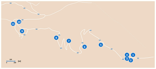
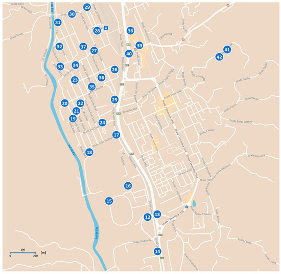
Figure 3.
The placement of monitoring points in the Rusu/Parâng areas, Brădet, and the Historic quarter/workers’ colony.

Table 1.
Sampling name/location of and/or air quality monitoring points in the areas of Rusu/Parâng, Brădet, the central-northern area of the Petroșani Municipality and the Historic quarter/workers’ colony.
The distribution of these measurement/monitoring points is as follows:
- 11 air quality determination points, numbered from 1 to 11, were placed in the Rusu/Parâng area;
- 26 air quality determination points, numbered from 12 to 37, were placed in the Historic quarter/workers’ colony;
- 5 air quality determination points, numbered from 38 to 42, were placed in the central-northern area of Petroșani Municipality and the Brădet area.
In the Parâng area, the measurements were carried out in a single session, during the winter, to capture any potential interference from pollution resulting from the heating of holiday homes/cabins in the area. In contrast, in the Historic quarter, the central-northern area, and the Brădet area, measurements were taken during the winter, both at night and during the day, to observe fluctuations in the concentration of pollutants or particulate matter when the population needed to use heating sources and when heating was not required.
2.3. Snow Sample Collection
All the instrumental measurements were conducted in 2023, while the determinations related to snow sample analysis were carried out in 2019 and 2023.
For determining air quality on the municipal ring road, the main intersections of this road were considered as monitoring points, materialized in the field at three locations: two at the ends and one in the central area.
The snow sampling activity, determinations, measurement, and pollutant monitoring took place in several stages, as follows:
- -
- 2–3 February 2019, snow sample collection, stage I;
- -
- 12–14 February 2023, snow sample collection, stage II;
- -
- February 2023, instrumental air determinations.
This resulted in 42 collection/measurement/monitoring points (Table 1) in the establishment of which all the pollution sources were taken into account. From 40 points, snow samples were collected in stage I, from 32 points, snow samples were collected in stage II, and in 42 of the points, only determinations of air quality were carried out.
We note that the first sampling stage 2–3 February 2019 was a trial stage to verify whether the results obtained through snow analysis can replace or complement instrumental measurements.
The difference between the number of snow samples collected in 2019 (40) and those collected in 2023 (32) resulted from the differences between the thickness of the snow layer and its persistence. For the same reason, different samplers were used in the two stages, the first one having a small diameter and a higher height and the second one having a large diameter and a lower height, because the snow layer was thicker in 2019 compared to 2023 and it was aimed to collect a sample volume as constant as possible (Table 1, Figure 4a).
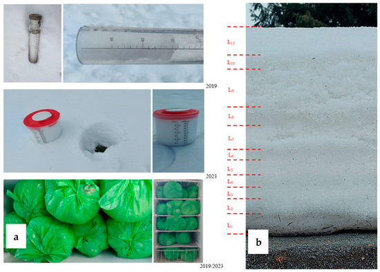
Figure 4.
Snow sample collection: (a) snow samplers and samples, (b) example of snow layers in Parâng area, 2023 campaign.
Snow is a natural filter that can collect pollutants from the air and store them until it melts [60,61,62,63]. This property makes snow a valuable tool for monitoring air pollution.
Air pollution monitoring through snow analysis is an effective method for measuring concentrations of atmospheric pollutants, including sulfur dioxide, nitrogen dioxide, and nitrogen oxides. Snow functions as an ideal sampling medium due to its inert nature, which allows it to retain pollutant deposits without alteration over time (Figure 4b).
2.4. Analytical Instruments and Parameters
In this work, the indirect methods of air quality analysis include the use of snow characteristics as an indicator of air pollution. By studying the physicochemical properties of the snow cover, relevant data on air composition and contamination levels in the area of interest can be obtained, providing an alternative and complementary perspective to instrumental monitoring methods. This approach allows for a detailed pollutant assessment, with the advantage of reflecting atmospheric pollutant accumulations over a longer period of time, which contributes to a deeper understanding of pollution dynamics in a particular mountain environment [64].
The following types of air pollutants can be monitored in snow:
Sulfur dioxide (SO2): SO2 can be converted to sulfuric acid (H2SO4) in snow, which changes the pH of the snow. By measuring the pH of the snow, the amount of SO2 in the air can be estimated.
Nitrogen oxides (NOx): NOx can be converted to nitric acid (HNO3) in snow, which changes the pH of the snow. By measuring the pH of the snow, the amount of NOx in the air can be estimated.
Particulate matter (PM): PM can be deposited directly on snow or incorporated into snow from the air. By measuring the concentration of PM in snow, the amount of PM in the air can be estimated [65].
There are two main methodologies for monitoring air pollution using snow [66,67,68,69,70]:
- Remote Sensing: Remote sensing techniques, including LiDAR and radar, can be employed to assess the depth and distribution of the snow layer. These data can then be utilized to estimate the quantity of pollutants that have been deposited within the snow.
- Field measurements: Snow samples can be collected from various locations and analyzed for pollutant concentrations. This data can be used to map the distribution of air pollutants.
Measurement of snow pH. One of the most common methods for monitoring air quality using snow is the measurement of snow pH [71,72]. Snow pH is an indicator of its acidity. Snowfall in unpolluted areas typically has a slightly alkaline pH, around 7.0. In polluted areas, the snow can have a more acidic pH, around 6.0 or lower.
Air pollutants such as sulfur and nitrogen oxides can react with water in the atmosphere to form sulfuric and nitric acids. These acids can dissolve salts from dust and particulate matter, increasing the concentration of acid salts in the snow. Also, this process can cause the snow to become more acidic [63,73,74,75,76,77].
By measuring the pH of snow, it is possible to estimate the amount of air pollutants present. Snow that falls in unpolluted areas typically has a slightly alkaline pH, around 7.0. This is because the water in the snow condenses around salts from the soil and rocks, which tend to have a slightly alkaline pH.
Acidic snow can have a range of negative consequences for the environment. It can affect the health of plants and animals, accelerate soil erosion, and damage concrete and stone structures. Monitoring the pH of snow is crucial for understanding the impact of air pollution on the environment. Such monitoring can help identify pollution sources and track changes in snow pH over time [69,74].
Examples of snow pH values are as follows:
- -
- Snow falling in unpolluted areas typically has a slightly alkaline pH, around 7.0.
- -
- Snow in polluted areas may have a more acidic pH, around 6.0 or lower.
- -
- Snow exposed to acid rain can have a very acidic pH, around 3.0 or lower.
Measurement of Pollutant Concentrations. In addition to measuring the pH of snow, other pollutant concentrations in snow can also be measured [25,61,78]. These pollutants include:
- -
- Sulfur dioxide (SO2)
- -
- Nitrogen oxides (NOx)
- -
- Particulate matter (PM)
These measurements can be performed using chemical or physical methods [79,80,81,82].
Solubility of NOx and SO2 in Snow. The solubility of NOx in snow is important for understanding the impact of air pollution on the environment. NOx can contribute to the formation of smog and sulfuric acid, which can have negative effects on health and the environment. Monitoring the solubility of NOx in snow can help identify air pollution sources and track changes in the concentration of NOx in the air over time. Monitoring air pollution with snow is an important method for understanding the impact of air pollution on the environment. It can be used to identify pollution sources and track changes in pollutant concentrations over time. The solubility of NOx in snow depends on several factors, including temperature, pH, and the concentration of NOx in the air. In general, NOx is more soluble in snow at lower temperatures and more alkaline pH levels. The concentration of NOx in the air is also an important factor determining its solubility in snow. At higher concentrations of NOx in the air, more NOx will be absorbed by the snow [83,84,85].
The solubility of atmospheric SO2 in snow depends on several factors, including temperature, pH, and the concentration of SO2 in the air. In general, SO2 is more soluble in snow at lower temperatures and more alkaline pH levels. The concentration of SO2 in the air is also a significant factor determining the solubility of SO2 in snow. At higher concentrations of SO2 in the air, more SO2 will be absorbed by the snow. Understanding the solubility of SO2 in snow is crucial for assessing the impact of air pollution on the environment. SO2 can contribute to the formation of sulfuric acid, which can have harmful effects on both health and the environment [86,87,88].
Particulate Matter. There are two main methods for monitoring air pollution using snow [62,68,89,90]:
1. Particle Extraction Method: This method involves collecting the snow and removing the pollutant particles from it. The particles can then be analyzed to determine the concentration of pollutants.
2. Absorption Measurement Method: This method involves measuring the amount of light absorbed by the snow. The concentration of pollutants can then be determined based on the amount of light absorbed.
Mineral Salts in Snow. The calcium and magnesium content of snow varies depending on location, season, and other factors such as air pollution [74,90,91]. Generally, snow that falls in mountainous areas contains higher levels of calcium and magnesium compared to snow in lowland areas. This is because the water that evaporates from the soil and rocks in mountainous regions contains more calcium and magnesium compounds [91]. Dissolved salts in snow are chemical compounds that dissolve in the water of the snow. These salts can come from natural sources, such as soil and rocks, or from anthropogenic sources, such as air pollution. Dissolved salts in snow are important for a range of ecological processes. They can affect the pH of the snow, contribute to ice formation, and influence the availability of nutrients for plants and animals [92,93,94].
Natural Sources of Dissolved Salts in Snow. Dissolved salts in snow can originate from natural sources such as soils and rocks. Soils and rocks contain a variety of salts, including chlorides, sulfates, phosphates, and nitrates. These salts can be transported into the atmosphere through processes like evaporation and condensation. When snow water condenses around these salts, they dissolve into the water [95,96].
Anthropogenic Sources of Dissolved Salts in Snow. Dissolved salts in snow can also come from anthropogenic sources, such as air pollution. Air pollutants like sulfur oxides and nitrogen oxides can react with water in the atmosphere to form sulfuric and nitric acids. These acids can dissolve salts from soils and rocks, increasing the concentration of dissolved salts in the snow. Monitoring dissolved salts in snow is crucial for understanding the impact of air pollution on the environment. This monitoring can help identify pollution sources and track changes in the concentration of dissolved salts in snow over time.
The calcium and magnesium content of snow can also be affected by air pollution. Air pollutants such as sulfur oxides and nitrogen oxides can react with water in the atmosphere to form sulfuric and nitric acids. These acids can dissolve calcium and magnesium from soils and rocks, increasing the calcium and magnesium content in the snow.
Typical concentrations of calcium and magnesium in snow are around 10 milligrams per liter for calcium and 5 milligrams per liter for magnesium. However, concentrations can vary significantly, reaching up to 100 milligrams per liter for calcium and 50 milligrams per liter for magnesium in mountainous areas [92,97].
Carrying out the monitoring of atmospheric pollutants through their accumulation in the snow layer requires the exact knowledge of the meteorological conditions during the period in which the tests were carried out using the data provided by the National Administration of Meteorology. The processed meteorological data are based on hourly measurements of temperature, wind direction, and speed, and measurements at 6 h intervals of precipitation volume and snow cover thickness.
The monitoring of atmospheric pollutants through their accumulation in the snow layer requires precise knowledge of the meteorological conditions during the period when the tests were conducted. The most important parameter in this case is the evolution of the snow layer that accumulated until the date the samples were taken.
It is essential to consider the thickness of the snow layer from the moment when a persistent layer began to form. The data indicating the start of persistent snow deposition are presented in Table 2.
Table 2.
The characteristics of the snow layer during the testing periods.
Table 2 also presents the characteristics of the deposited snow layer, as well as its evolution over time. It can be observed that in 2019, the snow layer persisted for 53 to 59 days until the sampling date, which allowed for a better accumulation of atmospheric pollutants compared to 2023, when the persistence period was only 18 to 35 days.
Table 3 presents the variation in air temperature during the accumulation period of the snow layer.
Table 3.
The variation in air temperature during the testing periods.
From Table 3, it can be observed that in 2019, the number of days in which the mini-mum temperature was above freezing represents 13.2% in Petroșani and 1.7% in Parâng. Additionally, the number of days in which the maximum temperature was above freezing represents 67.9% in Petroșani and 22.0% in Parâng. In contrast, in 2023, the number of days in which the minimum temperature was above freezing represents 0% in Petroșani and 2.9% in Parâng. Meanwhile, the number of days in which the maximum temperature was above freezing represents 77.8% in Petroșani and 40.0% in Parâng.
Table 4 presents the evolution of precipitation during the snow layer accumulation period.
Table 4.
The variation in precipitation during the testing periods.
As shown in Table 4, in 2019, the average daily precipitation was 5.2 mm in Petroșani and 5.1 mm in Parâng, corresponding to 75.5% of the monitored period in Petroșani and 81.4% in Parâng. In contrast, in 2023, the average daily precipitation was 4.9 mm in Petroșani and 11.0 mm in Parâng, accounting for 38.9% of the monitoring period in Petroșani and 68.6% in Parâng.
Table 5 illustrates the wind statistics during the snow accumulation period.
Table 5.
The characteristics of the winds during the testing periods.
As shown in Table 5, during the snow accumulation period, in all cases, the wind intensity did not exceed Beaufort scale grade 3 (light breeze), except for the 2023 sampling campaign in Parâng, where in 1.55% of the period, the wind exceeded grade 4 (moderate breeze), and only for 0.12% of the period (one hour) did the wind reach grade 5 (strong breeze). Based on these observations, it can be concluded that the wind did not significantly influence the deposition of the snow layer, as the conditions necessary for drifting snow were not met, except for the periods mentioned during the 2023 sampling campaign in Parâng, which accounted for 4 h, or 0.47% of the period (wind speeds greater than 25 km/h, or over 6.9 m/s).
2.5. Dispersion Model Description
Pollutant dispersion modeling in the atmosphere refers to the analysis of how pollutants spread in the air. Dispersion models are used to estimate the concentration, propagation direction, and potential accumulation areas of atmospheric pollutants emitted as a result of industrial activities, road traffic, or any construction activities [98,99,100].
From an ecological perspective, the danger of air pollution has two aspects: one direct, related to the atmospheric composition if it were to suffer short-term alterations, and another related to the role that the atmosphere can play as a vehicle for the rapid transport of many harmful factors (it acts as a vector for pollutants). The way pollutants disperse through the air depends on meteorological and geographical factors, as well as the quantity of pollutants emitted into the atmosphere.
To develop an atmospheric dispersion model, several factors must be considered: meteorological conditions (wind speed and direction, humidity, temperature), geographical conditions of the area where the sources and receptors are located (topography, land use patterns), emission parameters (location and height of sources, stack diameter, for example), and obstruction sources (buildings or other structures). Wind is the most important factor contributing to the dispersion of pollutants in the atmosphere. It manifests as a horizontal movement of the atmosphere, which carries pollutants within the air masses moved by the wind. The diffusion of pollutants in the atmosphere is directly proportional to wind speed. Light and steady winds maintain high pollutant concentrations in the air layer they have reached. The higher the wind speed, the greater the volume of air in which the pollutant disperses, and the resulting concentrations will be lower. Therefore, wind is a positive factor in the fight against the accumulation of pollutants, but it is also responsible for the unwanted dispersion of pollutants from the ground. Atmospheric calm is the most favorable meteorological condition for air pollution because, as pollutants are produced by various sources, they accumulate near the emission point, and their concentration continuously increases.
Air turbulence is a complex phenomenon resulting from differences in temperature, movement, and friction between layers of moving air, which causes a continuous state of internal agitation in small portions of air masses. Turbulence promotes the crosswind dispersion of pollutants, and it is directly related to the wind regime. Strong turbulence is characterized by significant fluctuations in wind direction and speed at the surface, which mix the air thoroughly. In the case of moderate turbulence, characterized by neutral vertical stability, wind fluctuations are smaller. Meanwhile, in weak turbulence, with vertical stability, the wind is weak and constant in both direction and intensity.
Atmospheric humidity is a climatic factor that has an unfavorable impact on the dispersion and transport of pollutants. On the contrary, it sometimes contributes to the formation of very harmful effects on life, such as fog and even smog. Precipitation, in contrast to fog, helps with the dispersion and transport of pollutants in the atmosphere; however, it negatively affects the soil and water, as all pollutants reach these components, where they infiltrate, altering their properties, thus leading to a pollution phenomenon. Clouds, as a compact, static, and low-altitude layer, create an enclosed space where the dispersion and transport of pollutants are not favored. However, when they form a discontinuous and constantly moving layer, they promote the dispersion and transport of pollutants.
As observed, climatic factors have a significant influence on the dispersion and transport of pollutants. Their importance is even greater given their ability to transform a life-friendly environment into one that is totally hostile, and vice versa. Therefore, nature can be both a friend and an enemy, which is why it is important to understand it and live in perfect harmony with its rules, for the benefit of human society, since the injustice is caused by us, not by nature.
Air pollutant dispersion modeling is performed using computer programs called dispersion models, which solve the equations and algorithms that simulate the dispersion of pollutants. Dispersion models are used to estimate or forecast the concentration of atmospheric pollutants emitted by various sources, such as industrial facilities or road traffic. Such models are important for government agencies responsible for protecting and managing air quality. They are typically used to determine whether existing or newly proposed industrial installations comply with current air quality standards. Models also serve to design effective control strategies for reducing harmful atmospheric pollutants.
Dispersion models require the following input data:
- Meteorological conditions, such as wind speed and direction, atmospheric turbulence levels characterized by what is called the stability class, air temperature, and the altitude of any thermal inversion base, if present.
- Emission parameters, including the location and height of the source, the diameter of the emission mouth, the velocity of the pollutant jet, the exit temperature, and the mass flow rate of the pollutant.
- Terrain elevation at the location of both the source and the receptor.
- Location, height, and width of any obstacles (such as buildings or other structures) in the path of the gas emission plume.
Advanced dispersion modeling programs typically include a preprocessing module for entering meteorological and other input data, and a postprocessing module for graphical representation of output data, including mapping the affected areas by air pollution on various maps.
To calculate the pollutant concentrations in the air generated by one or more atmospheric emission sources, spatial modeling methodologies are applied, utilizing professional software packages simulating and predicting the dispersion of pollutants, enabling the assessment of their impact on air quality and providing valuable information for air quality and regulatory purposes [70].
3. Results and Discussions
3.1. Spatial Distribution of Pollutants
As previously mentioned, during the cold season, 11 air quality monitoring points were set in the Rusu/Parâng area, numbered from 1 to 11 (Table S1). The measurements were taken in a single session, during winter, in the daytime (☼), to capture any potential interference from pollution resulting from the heating of holiday homes/cabins in the area.
As a result of the analysis of pollution sources, it was found that the Historic quarter/workers’ colony is the most polluted area of the Municipality of Petroșani (Table S2). Consequently, the highest number of air quality monitoring points, 26 in total, was set in this area. These were numbered from 12 to 37. Additional measurements were taken in the central-northern part of the municipality, where there is direct exposure to the historic area, to capture any negative influences on air quality caused by pollutants emitted from the homes in the former workers’ colony. Measurements were also made in the Brădet area, located at a higher altitude than the City center, where a few villas are increasingly immersed in nature. These five monitoring points were numbered from 38 to 42 (Table S3). All of these measurements were conducted during the cold season, both at night (☽) and during the day (☼), for the reasons stated above [4].
For instrumental measurements conducted in the winter of 2023, the following average values were obtained (Table 6):
Table 6.
Average values of instrumental measurements conducted, Winter 2023.
The data reveal a similar trend in the behavior of gaseous pollutants and fine particulate matter:
- Gaseous substances exhibit a decreasing trend in the order of Historic quarter → City center → Parâng, as illustrated in Figure 5 for TVOC (Total Volatile Organic Compounds).
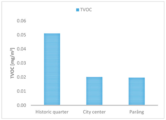 Figure 5. Variation of TVOC parameter values in the three measurement areas.
- Suspended particles also show a decreasing trend in the same order, as exemplified in Figure 6 for PM1, PM2.5, and PM10.
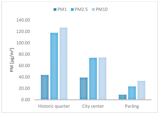 Figure 6. Variation of suspended particles values in the three measurement areas.
The similar behavior of gaseous pollutants and suspended particles is attributed to common factors influencing their dispersion:
- Air Movements (Convection and Turbulence): Both gaseous pollutants and suspended particles are transported by air currents. Atmospheric convection lifts them to higher altitudes or disperses them horizontally, while atmospheric turbulence, driven by temperature and wind variations, facilitates their mixing and uniform distribution in the air.
- Wind and Long-Range Transport: Pollutants can be carried over long distances by wind, leading to the contamination of areas far from the pollution source. Larger particles (PM10) tend to settle more quickly, whereas finer particles (PM2.5 and PM0.1—nanoparticles) and gaseous pollutants remain air-borne for longer periods and may be transported hundreds or even thousands of kilometers.
- Atmospheric Diffusion: Both gases and ultrafine particles disperse due to random molecular motion in the air (Brownian diffusion), contributing to their homogenization in the atmosphere.
- Atmospheric Stratification: Under thermal inversion conditions, cold air near the surface becomes trapped beneath a layer of warmer air, preventing pollutant dispersion and leading to their accumulation at ground level. This phenomenon similarly affects both gaseous pollutants (e.g., NO2, SO2) and fine particles, resulting in increased local concentrations.
3.2. Temporal Trends
In the historic neighborhood, the central-northern area, and Brădet, the air quality measurements taken during the cold season were conducted both at night and during the day. This approach aimed to capture fluctuations in the concentration of pollutants or suspended particles when the population was required to use heating sources, as well as during times when heating was not necessary.
For comparison, Figure 7 and Figure 8 present the average values of the measurements taken in the two areas.

Figure 7.
Comparison of the concentrations of particulate matters, based on the average values of measurements taken (day and night) in the Historic quarter, compared to those in the City center.
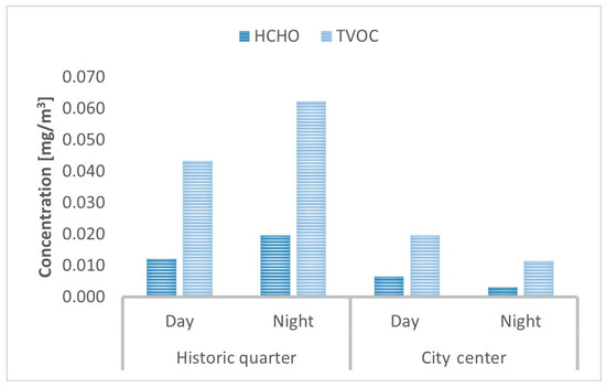
Figure 8.
Comparison of the concentrations of volatile organic compounds and formaldehyde, based on the average values of measurements taken (day and night) in the Historic quarter, compared to those in the City center.
The two diagrams indicate that in the Historic quarter, the average concentrations of the monitored pollutants are 2.8 to 3.5 times higher during the day and 0.7 to 1.3 times higher in the night for particulate matter, whereas for volatile organic compounds (VOCs), the concentrations are 1.8 to 2.2 times higher during the day and 5.4 to 6.1 times higher in the night in the Historic quarter compared to the City center.
Air quality data measured in the Rusu/Parâng area and in the historical districts of Petroșani highlight significant differences between daytime and nighttime measurements, as well as between the different monitored areas. It was observed that in residential areas, especially in the Historic quarter, the values of PM10, CO2, and volatile organic compounds (VOCs) were higher at night, suggesting a strong influence from domestic heating sources. This phenomenon was less evident in more isolated areas, such as Parâng.
3.3. Snow Chemistry Analysis
The results obtained for snow sample determinations (Tables S4 and S5) and instrumental measurements were averaged to facilitate comparison. Thus, for the determinations performed on snow samples in 2023, the following average values were obtained for the measured parameters: TDS (Total Dissolved Solids), Conductivity, Sediment, Ca2+, Mg2+, and SO42− (Table 7).
Table 7.
Average values of determinations performed on snow samples, Winter 2023.
From the data presented in the table above, two types of trends emerge:
- For substances dissolved in snow water, a decreasing trend is observed in the order of Historic quarter → City center → Parâng, as illustrated in Figure 9 for TDS.
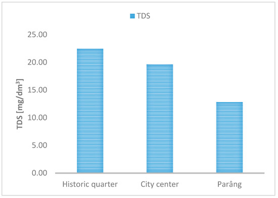 Figure 9. Variation of TDS parameter values across the measurement areas.
- 2
- For substances deposited by sedimentation from the air, an increasing trend is observed in the same order, as exemplified in Figure 10 for sediment.
 Figure 10. Variation of sediment parameter values across the measurement areas.
These differing trends can be explained by the distinct mechanisms of substance retention in snow. Dissolved substances primarily originate from gaseous pollution, including sulfur dioxide (SO2), nitrogen oxides (NOx), ammonia (NH3), and other polluting gases, as well as soluble aerosols (mainly salts of alkali and alkaline earth metals). These dissolve in atmospheric water droplets or snow, forming acids (e.g., sulfuric acid, nitric acid) and other soluble compounds.
Solid particles come from sources such as fossil fuel combustion, the metallurgical industry, construction activities, and soil dust. These particles are insoluble or only partially soluble and may contain heavy metals, soot, sand particles, and dust.
Transport and deposition mechanisms vary depending on the nature of the sub-stances, as follows:
- Wet deposition is characteristic of gaseous pollutants and soluble aerosols, which dissolve in atmospheric water droplets or ice crystals and are transported with precipitation. This process increases the concentration of dissolved substances in snow.
- Dry deposition involves larger solid particles (PM10, PM2.5) that settle by gravity or are transported by wind, adhering to the snow surface. These do not dissolve immediately and may remain as visible particles.
These processes are influenced by meteorological factors as follows:
- Low temperatures reduce the solubility of certain gases, which may lead to a discrepancy between the concentration of dissolved substances and that of solid particles.
- Wind intensity affects the transport of solid particles and can result in greater accumulation in specific areas.
Atmospheric humidity influences the air’s capacity to retain soluble gases before they are incorporated into precipitation.
Physicochemical Processes in Snow. After snowfall, snow continues to interact with both the atmosphere and the soil. Dissolved substances may undergo chemical reactions, be absorbed by ice crystals, or be released into the air during melting. In contrast, solid particles typically remain trapped in the snow until it melts, at which point they are either released into the water or left behind as a layer of residue.
The persistence of the snow layer was significantly greater in 2019 than in 2023, which favored a higher accumulation of atmospheric pollutants.
The higher temperatures in 2023 contributed to a more rapid melting of the snow layer, thereby influencing the chemical composition of the analyzed samples.
3.4. Impact of Meteorological Factors
The analysis of the snow layer from the monitoring campaigns of 2019 and 2023 reveals significant differences in terms of pollutant accumulation periods. In 2019, the snow cover persisted for a longer period (53–59 days), providing a greater interval for the accumulation of atmospheric pollutants, compared to 2023, when the persistence period was shorter (18–35 days). This difference can significantly influence the concentrations of pollutants identified in the snow samples.
Air temperature played a crucial role in the accumulation and retention of snow. In 2019, average temperatures were lower, with fewer days where the minimum temperature exceeded 0 °C. This factor contributed to maintaining a stable snow layer, minimizing freeze–thaw cycles that could influence the distribution and chemical composition of retained pollutants.
In 2023, elevated temperatures, coupled with an increased number of days with above-freezing conditions, contributed to a decrease in snow persistence, thereby influencing both the concentration of pollutants within the snow and their dispersion in the environment.
Another significant factor was the level of precipitation. In 2019, the number of days with substantial precipitation (>5 mm and >10 mm) was higher compared to 2023. This resulted in increased water accumulation within the snow layer, which may dilute certain chemical compounds while also enhancing the retention of atmospheric particles.
Wind speed data indicate that, overall, conditions were not conducive to significant pollutant dispersion through the resuspension of particles from the snow layer. However, during the 2023 campaign in Parâng, there were fewer hours in which wind speeds exceeded the thresholds defined by the Beaufort scale, suggesting a limited influence of wind on pollutant redistribution.
The analysis of the snow layer composition shows significant variations between 2019 and 2023 in terms of chemical pollutant concentrations and physicochemical parameters. In 2019, higher values of sediments, TDS (Total Dissolved Solids), and conductivity were recorded, suggesting a greater accumulation of atmospheric particles and dissolved substances in the snow. In contrast, in 2023, the lower values of these parameters may be linked to a shorter accumulation period and the potential impact of higher temperatures.
Precipitation levels and wind speed had different impacts on pollutant dispersion and accumulation in each campaign.
3.5. Dispersion Model Interpretation
The modeling of atmospheric pollutant dispersion emphasizes the impact of meteorological factors on their distribution. Under low wind and low-temperature conditions, pollutants tend to accumulate near the ground, deteriorating air quality in residential areas. Conversely, stronger winds facilitate greater pollutant dispersion, potentially lowering local concentrations while contributing to their transport to other regions.
Pollutant dispersion maps (Figure 11, Figure 12, Figure 13 and Figure 14) show that during the cold season, PM10 and TVOC (Total Volatile Organic Compounds) concentrations are higher at night, indicating a significant effect of human activities (domestic heating) on air pollution.

Figure 11.
PM10 map, comparative winter measurements, day/night.
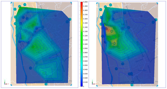
Figure 12.
TVOC map, comparative winter measurements, day/night.
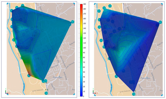
Figure 13.
TDS map, comparative measurements 2019/2023.
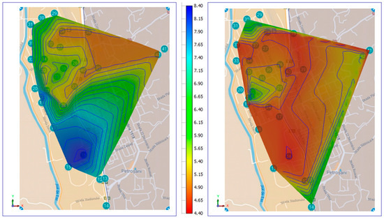
Figure 14.
pH map, comparative measurements 2019/2023.
The modeling of pollutant dispersion confirms the importance of meteorological fac-tors in their distribution and highlights the need for air quality management measures according to atmospheric conditions.
3.6. Comparison Between Instrumental Air Quality Monitoring and Pollutant Determination in Snow
Air quality monitoring and the determination of pollutants in snow are two complementary methods used to assess atmospheric pollution levels. Each method has its own advantages, disadvantages, and specific applications, and a comparison between the two can highlight their relevance in the context of air quality monitoring.
Instrumental air quality monitoring relies on the use of specialized equipment, such as sensors and automatic analyzers, to measure atmospheric pollutant concentrations in real time. The measured parameters include suspended particles (PM10, PM2.5, PM1), carbon dioxide (CO2), formaldehyde (HCHO), volatile organic compounds (VOCs), and other gaseous pollutants (SO2, NOx, O3). The equipment is installed at fixed or mobile points and provides continuous, day-and-night measurements.
The determination of pollutants in snow is based on the collection of snow samples and their laboratory analysis to determine the concentrations of accumulated chemical pollutants and particles. This method assumes that snow acts as a “natural filter” that captures atmospheric pollutants during precipitation and direct deposition from the air.
Analyzed parameters include pH, electrical conductivity, TDS (Total Dissolved Sol-ids) content, specific ions (Ca2+, Mg2+, SO42−), sediments, and heavy metals (Table 8).
Table 8.
Comparison between instrumental air quality monitoring and pollutant determination in snow.
Instrumental air quality monitoring is ideal for detecting pollution episodes and evaluating daily or hourly pollutant concentration fluctuations. This type of monitoring is essential for implementing air quality policies, issuing alerts, and protecting the population in cases of acute pollution episodes. It allows differentiation between short-term pollution sources (traffic, industry) and chronic ones (domestic heating).
The determination of pollutants in snow is more suitable for evaluating long-term pollutant accumulation and for environmental impact studies, especially in mountainous or peri-urban areas where the snow layer persists. This method provides a cumulative picture of pollution, integrating atmospheric influences over deposition periods. It is useful for investigating pollution effects on aquatic ecosystems, soil, and vegetation, as melted snow can transport pollutants into these environments.
Both methods complement each other rather than being mutually exclusive. Instrumental monitoring provides detailed real-time data on air quality, while snow pollutant analysis offers insight into long-term pollutant accumulation and distribution during the cold season. Together, these methods can provide essential information for a deeper understanding of atmospheric pollution dynamics and for developing effective environ-mental and public health protection strategies.
The analysis of air quality monitoring results reveals significant variations in pollutant concentrations between sampling points, as well as across different time intervals. This high variability underscores the need for complementary monitoring methods, particularly during the cold season. One effective approach could be snow analysis, which can provide additional insights into deposited atmospheric pollutants and their medium-term accumulation. This method would enable a clearer estimation of the impact of emissions on the environment and public health, especially in areas with multiple pollution sources, such as heavy traffic and residential heating with solid fuels.
The use of snow analysis could help determine pollutant accumulation during the cold season, offering a more comprehensive perspective on long-term impacts. Thus, in addition to conventional air quality monitoring, investigating pollutants accumulated in snow can provide valuable information and contribute to a better understanding of atmospheric pollution dynamics during winter.
Air quality was strongly influenced by human activities, with notable differences between daytime and nighttime measurements, especially in residential areas.
These conclusions underscore the importance of continuous air quality and snow layer monitoring to better understand the impact of pollution on the environment and human health.
4. Conclusions
In the heart of the Petroșani Mountain Depression, where the air still bears the imprint of a long industrial history, this study aims to provide a clear picture of how air pollutants are distributed and evolve over time. This study proposes an integrated methodology that combined conventional air quality monitoring methods with a more sustainable approach—analyzing the chemical composition of snow, a natural filter that traps particles in the atmosphere. With this dual methodology, this study explores the effectiveness of snow analysis as a sustainable and complementary alternative to instrumental measurements, especially in mountainous regions where the infrastructure for continuous monitoring is limited. At the same time, this study investigates the link between pollution sources and the atmospheric processes that determine the dispersion and accumulation of pollutants in these kinds of areas. Snow serves as a valuable natural medium for monitoring air pollution, offering advantages such as long-term pollutant storage, cost-effectiveness, and widespread availability across diverse geographic regions.
Another key aspect of the research is assessing the influence of meteorological factors on pollutant accumulation. Comparisons between years with different climatic conditions allow a better understanding of the impact of temperature, precipitation, and air circulation on air pollution.
However, several challenges must be addressed, including pollutant release during snowmelt, long-range transport of contaminants, and variations in snow quality, which can complicate data interpretation and source attribution.
Ultimately, this study emphasizes the need for diverse and adaptable air quality monitoring strategies. In mountainous regions where pollution monitoring faces logistical challenges, combining snow analysis with instrumental methods provides a fuller picture of environmental contamination. By leveraging both approaches, policymakers and researchers can better assess air quality trends, mitigate pollution risks, and protect both ecosystems and public health.
Supplementary Materials
The following supporting information can be downloaded at: https://www.mdpi.com/article/10.3390/su17073141/s1, Table S1: Air quality measurements in the Rusu area and Parâng Mountains, on March 5, 2023; Table S2: Air quality measurements in the Historic quarter, on March 07, 08, 09 and 10, 2023; Table S3: Air quality measurements in the central-northern area and Brădet Hill, on March 08 and 09, 2023; Table S4: Analysis of snow quality parameters in 2019; Table S5: Analysis of snow quality parameters in 2023.
Author Contributions
Conceptualization, C.L.; methodology, C.L., E.T., S.M.R. and D.M.; software, A.F.; validation, C.L., S.M.R. and E.T.; formal analysis, C.L. and E.T.; investigation, C.L., A.F., A.N. and E.R.; data curation, C.L., E.T., D.M., A.N. and E.R.; writing—original draft preparation, C.L.; writing—review and editing, C.L., E.T. and D.M.; funding acquisition, C.L. All authors have read and agreed to the published version of the manuscript.
Funding
This research was funded through the UNIVERSITY OF PETROSANI Scientific Research Contract (CIFC 6—CCGUEUST) No. 4282, dated 31 May 2023, led by Assoc. Prof. Dr. Eng. Csaba LORINŢ. Topic: Comparative study of urban geology, human ecology, and traffic patterns with an impact on air quality in Petroșani Municipality within the context of decarbonization of mining areas.
Institutional Review Board Statement
Not applicable.
Informed Consent Statement
Not applicable.
Data Availability Statement
The data presented in this study are available on request from the corresponding author.
Conflicts of Interest
The authors declare no conflicts of interest.
Abbreviations
The following abbreviations are used in this manuscript:
| PM | Particulate Matter |
| HCHO | Formaldehyde |
| TDS | Total Dissolved Solids |
| VOCs | Volatile Organic Compounds |
| TVOC | Total Volatile Organic Compounds |
References
- Calamar, A.-N.; Gaman, G.A.; Pupazan, D.; Toth, L.; Kovacs, I. Analysis of environmental components by monitoring gas concentrations in the environment. Environ. Eng. Manag. J. 2017, 16, 1249–1256. [Google Scholar] [CrossRef]
- Sharma, A.; Mitra, A.; Sharma, S.; Roy, S. Estimation of Air Quality Index from Seasonal Trends Using Deep Neural Network. In Artificial Neural Networks and Machine Learning–ICANN 2018: 27th International Conference on Artificial Neural Networks, Rhodes, Greece, October 4–7, 2018, Proceedings, Part III; Springer: Berlin/Heidelberg, Germany, 2018; pp. 511–521. [Google Scholar] [CrossRef]
- Taştan, M.; Gökozan, H. Real-Time Monitoring of Indoor Air Quality with Internet of Things-Based E-Nose. Appl. Sci. 2019, 9, 3435. [Google Scholar] [CrossRef]
- Lorinț, C.; Danciu, C.; Traistă, E.; Florea, A.; Rezmerița, E. Aspects regarding the impact of cloth waste burning in the historical residential areas of the Petroșani municipality. MATEC Web Conf. 2024, 389, 83. [Google Scholar] [CrossRef]
- Wang, Q.; Ao, R.; Chen, H.; Li, J.; Wei, L.; Wang, Z. Characteristics of PM2.5 and CO2 Concentrations in Typical Functional Areas of a University Campus in Beijing Based on Low-Cost Sensor Monitoring. Atmosphere 2024, 15, 1044. [Google Scholar] [CrossRef]
- Afifa; Arshad, K.; Hussain, N.; Ashraf, M.H.; Saleem, M.Z. Air pollution and climate change as grand challenges to sustainability. Sci. Total Environ. 2024, 928, 172370. [Google Scholar] [CrossRef]
- Neira, M.; Prüss-Ustün, A.; Mudu, P. Reduce air pollution to beat NCDs: From recognition to action. Lancet 2018, 392, 1178–1179. [Google Scholar] [CrossRef]
- Chukwu, T.M.; Morse, S.; Murphy, R.J. Spatial Analysis of Air Quality Assessment in Two Cities in Nigeria: A Comparison of Perceptions with Instrument-Based Methods. Sustainability 2022, 14, 5403. [Google Scholar] [CrossRef]
- Word Health Organization. WHO Global Air Quality Guidelines: Particulate Matter (PM2.5 and PM10), Ozone, Nitrogen Dioxide, Sulfur Dioxide and Carbon Monoxide; World Health Organization: Geneva, Switzerland, 2021; ISBN 978-92-4-003422-8. Available online: https://iris.who.int/handle/10665/345329 (accessed on 19 March 2025).
- Rezmerița, E.; Radu, S.M.; Călămar, A.-N.; Lorinț, C.; Florea, A.; Nicola, A. Urban Air Quality Monitoring in Decarbonization Context; Case Study—Traditional Coal Mining Area, Petroșani, Romania. Sustainability 2022, 14, 8165. [Google Scholar] [CrossRef]
- Sustainable Development Goal Indicator 3.9.1: Mortality Attributed to air Pollution [Internet]. Available online: https://www.who.int/publications/i/item/9789240099142 (accessed on 19 March 2025).
- Leung, D.Y.C. Outdoor-indoor air pollution in urban environment: Challenges and opportunity. Front. Environ. Sci. 2015, 2, 69. [Google Scholar] [CrossRef]
- Azuma, K.; Kagi, N.; Yanagi, U.; Osawa, H. Effects of low-level inhalation exposure to carbon dioxide in indoor environments: A short review on human health and psychomotor performance. Environ. Int. 2018, 121, 51–56. [Google Scholar] [CrossRef]
- Kampa, M.; Castanas, E. Human health effects of air pollution. Environ. Pollut. 2008, 151, 362–367. [Google Scholar] [CrossRef] [PubMed]
- Lelieveld, J.; Evans, J.S.; Fnais, M.; Giannadaki, D.; Pozzer, A. The contribution of outdoor air pollution sources to premature mortality on a global scale. Nature 2015, 525, 367–371. [Google Scholar] [CrossRef] [PubMed]
- Cohen, A.J.; Brauer, M.; Burnett, R.; Anderson, H.R.; Frostad, J.; Estep, K.; Balakrishnan, K.; Brunekreef, B.; Dandona, L.; Dandona, R.; et al. Estimates and 25-year trends of the global burden of disease attributable to ambient air pollution: An analysis of data from the Global Burden of Diseases Study 2015. Lancet 2017, 389, 1907–1918. [Google Scholar] [CrossRef]
- Annesi-Maesano, I.; Baiz, N.; Banerjee, S.; Rudnai, P.; Rive, S.; Sinphonie Group. Indoor Air Quality and Sources in Schools and Related Health Effects. J. Toxicol. Environ. Health Part B 2013, 16, 491–550. [Google Scholar] [CrossRef]
- Chapman, E.G.; Gustafson, W.I.J.; Easter, R.C.; Barnard, J.C.; Ghan, S.J.; Pekour, M.S.; Fast, J.D. Coupling aerosol-cloud-radiative processes in the WRF-Chem model: Investigating the radiative impact of elevated point sources. Atmos. Chem. Phys. 2009, 9, 945–964. [Google Scholar] [CrossRef]
- Dong, F.; Yu, B.; Pan, Y. Examining the synergistic effect of CO2 emissions on PM2.5 emissions reduction: Evidence from China. J. Clean. Prod. 2019, 223, 759–771. [Google Scholar] [CrossRef]
- Yang, S.; Chen, B.; Ulgiati, S. Co-benefits of CO2 and PM2.5 Emission Reduction. Energy Procedia 2016, 104, 92–97. [Google Scholar] [CrossRef]
- Rojas González, L.; Montilla-Rosero, E. Evaluation of In-Situ Low-Cost Sensor Network in a Tropical Valley, Colombia. Sensors 2025, 25, 1236. [Google Scholar] [CrossRef]
- Zhan, C.; Xie, M.; Lu, H.; Liu, B.; Wu, Z.; Wang, T.; Zhuang, B.; Li, M.; Li, S. Impacts of urbanization on air quality and the related health risks in a city with complex terrain. Atmos. Chem. Phys. 2023, 23, 771–788. [Google Scholar] [CrossRef]
- Yarce Botero, A.; Lopez Restrepo, S.; Sebastian Rodriguez, J.; Valle, D.; Galvez-Serna, J.; Montilla, E.; Botero, F.; Henzing, B.; Segers, A.; Heemink, A.; et al. Design and Implementation of a Low-Cost Air Quality Network for the Aburra Valley Surrounding Mountains. Pollutants 2023, 3, 150–165. [Google Scholar] [CrossRef]
- Martínez, J.; Olaya Morales, Y.; Kumar, P. Spatial and temporal variability of urban cyclists’ exposure to PM2.5 in Medellín, Colombia. Atmos. Pollut. Res. 2024, 15, 101946. [Google Scholar] [CrossRef]
- Sakai, H.; Sasaki, T.; Saito, K. Heavy metal concentrations in urban snow as an indicator of air pollution. Sci. Total Environ. 1988, 77, 163–174. [Google Scholar] [CrossRef] [PubMed]
- Munawer, M.E. Human health and environmental impacts of coal combustion and post-combustion wastes. J. Sustain. Min. 2018, 17, 87–96. [Google Scholar] [CrossRef]
- Amoatey, P.; Omidvarborna, H.; Baawain, M.S.; Al-Mamun, A. Emissions and exposure assessments of SOX, NOX, PM10/2.5 and trace metals from oil industries: A review study (2000–2018). Process Saf. Environ. Prot. 2019, 123, 215–228. [Google Scholar] [CrossRef]
- Koshland, C.P. Impacts and control of air toxics from combustion. Symp. (Int.) Combust. 1996, 26, 2049–2065. [Google Scholar] [CrossRef]
- Durmishi, B.H.; Durmishi, A.; Shabani, A. The role of instrumental methods in chemical analysis for environmental protection. Int. J. Chem. Mater. Sci. (IJCMS) 2025, 10, 1–22. [Google Scholar] [CrossRef]
- Beck, D.; Mitkiewicz, J. A systematic literature review of citizen science in urban studies and regional urban planning: Policy, practical, and research implications. Urban Ecosyst. 2025, 28, 85. [Google Scholar] [CrossRef]
- Marenaci, P.; Otal, L.E. Sentinel 4: A geostationary imaging UVN spectrometer for air quality monitoring: Optical alignment of the Instrument Flight Model 2. In Proceedings of the Optical Design and Engineering IX, Strasbourg, France, 7–12 April 2024; Volume 13019, pp. 253–271. Available online: https://www.spiedigitallibrary.org/conference-proceedings-of-spie/13019/1301918/Sentinel-4--a-geostationary-imaging-UVN-spectrometer-for-air/10.1117/12.3017155.full (accessed on 19 March 2025).
- Ajibola, A.S.; Adeshina, S.; Ojo, T.O. Levels and ecological risk assessment of UV filters in sediments of Odo-Iyaalaro River and Eleyele Lake, Nigeria. Discov. Environ. 2025, 3, 32. [Google Scholar] [CrossRef]
- Barro, R.; Regueiro, J.; Llompart, M.; Garcia-Jares, C. Analysis of industrial contaminants in indoor air: Part 1. Volatile organic compounds, carbonyl compounds, polycyclic aromatic hydrocarbons and polychlorinated biphenyls. J. Chromatogr. A 2009, 1216, 540–566. [Google Scholar] [CrossRef]
- Santamaría, C.; Elustondo, D.; Lasheras, E.; Santamaría, J.M. Air Pollutants in the Outdoor Environment (NOx, SO2, VOCs, HAPs [CO, O3]). In Chromatographic Analysis of the Environment; CRC Press: Boca Raton, FL, USA, 2017; ISBN 978-1-315-31620-8. [Google Scholar]
- Ntesat, U.B.; Bright, N.; Chima, D.I.; Ayotamuno, M.J. Investigation of the Level of Air Pollution Caused by Crude Oil Production and its Health Effects on the Inhabitants of the Production Area. Int. J. Eng. Inf. Syst. (IJEAIS) 2024, 8, 25–31. [Google Scholar]
- Sa’adeh, H.; Chiari, M. Characterization of particulate matter (PM2.5 and PM10) in an urban area in Amman by PIXE, PESA, optical and gravimetric measurements. Nucl. Instrum. Methods Phys. Res. Sect. B Beam Interact. Mater. At. 2024, 553, 165388. [Google Scholar] [CrossRef]
- Saporito, A.F.; Gordon, T.; Kim, B.; Huynh, T.; Khan, R.; Raja, A.; Terez, K.; Camacho-Rivera, N.; Gordon, R.; Gardella, J.; et al. Skyrocketing pollution: Assessing the environmental fate of July 4th fireworks in New York City. J. Expo. Sci. Environ. Epidemiol. 2024, 1–9. [Google Scholar] [CrossRef] [PubMed]
- Borhan, M.S.; Khanaum, M.M. Sensors and Methods for Measuring Greenhouse Gas Emissions from Different Components of Livestock Production Facilities. J. Geosci. Environ. Prot. 2022, 10, 242–272. [Google Scholar] [CrossRef]
- Ma, W.; Ji, X.; Ding, L.; Yang, S.X.; Guo, K.; Li, Q. Automatic Monitoring Methods for Greenhouse and Hazardous Gases Emitted from Ruminant Production Systems: A Review. Sensors 2024, 24, 4423. [Google Scholar] [CrossRef]
- Sobus, J.R.; Sayre-Smith, N.A.; Chao, A.; Ferland, T.M.; Minucci, J.M.; Carr, E.T.; Brunelle, L.D.; Batt, A.L.; Whitehead, H.D.; Cathey, T.; et al. Automated QA/QC reporting for non-targeted analysis: A demonstration of “INTERPRET NTA” with de facto water reuse data. Anal. Bioanal. Chem. 2025, 417, 1897–1914. [Google Scholar] [CrossRef]
- Jin, D.; Lu, Z.; Song, X.; Ahammed, G.J.; Yan, Y.; Chen, S. Improvement of Yield and Quality Properties of Radish by the Organic Fertilizer Application Combined with the Reduction of Chemical Fertilizer. Agronomy 2024, 14, 1847. [Google Scholar] [CrossRef]
- Bellini, A.; Diémoz, H.; Di Liberto, L.; Gobbi, G.P.; Bracci, A.; Pasqualini, F.; Barnaba, F. ALICENET—An Italian network of automated lidar ceilometers for four-dimensional aerosol monitoring: Infrastructure, data processing, and applications. Atmos. Meas. Tech. 2024, 17, 6119–6144. [Google Scholar] [CrossRef]
- Johann, S.; Düster, M.; Bellanova, P.; Schwarzbauer, J.; Weber, A.; Wolf, S.; Schüttrumpf, H.; Lehmkuhl, F.; Hollert, H. Dioxin-like and estrogenic activity screening in fractionated sediments from a German catchment after the 2021 extreme flood. Environ. Sci. Eur. 2024, 36, 163. [Google Scholar] [CrossRef]
- Zhang, Y.; Zhao, T.; Sun, X.; Bai, Y.; Shu, Z.; Fu, W.; Lu, Z.; Wang, X. Ozone pollution aggravated by mountain-valley breeze over the western Sichuan Basin, Southwest China. Chemosphere 2024, 361, 142445. [Google Scholar] [CrossRef]
- Popescu, F.D.; Radu, S.M.; Andras, A.; Brinas, I.; Marita, M.-O.; Radu, M.A.; Brinas, C.L. Stability Assessment of the Dam of a Tailings Pond Using Computer Modeling—Case Study: Coroiești, Romania. Appl. Sci. 2024, 14, 268. [Google Scholar] [CrossRef]
- Planchon, F.A.M.; Boutron, C.F.; Barbante, C.; Cozzi, G.; Gaspari, V.; Wolff, E.W.; Ferrari, C.P.; Cescon, P. Changes in heavy metals in Antarctic snow from Coats Land since the mid-19th to the late-20th century. Earth Planet. Sci. Lett. 2002, 200, 207–222. [Google Scholar] [CrossRef]
- Baltrėnas, P.; Baltrėnaitė, E. Natural and Semi-Natural Biogeochemical Barriers as Natural Technologies. In Sustainable Environmental Protection Technologies: Contaminant Biofiltration, Adsorption and Stabilization; Baltrėnas, P., Baltrėnaitė, E., Eds.; Springer International Publishing: Cham, Switzerland, 2020; pp. 39–91. ISBN 978-3-030-47725-7. [Google Scholar]
- Krastinytė, V.; Baltrėnaitė, E.; Lietuvninkas, A. Analysis of snow-cap pollution for air quality assessment in the vicinity of an oil refinery. Environ. Technol. 2013, 34, 757–763. [Google Scholar] [CrossRef] [PubMed]
- Muir, D.; Gunnarsdóttir, M.J.; Koziol, K.; von Hippel, F.A.; Szumińska, D.; Ademollo, N.; Corsolini, S.; Silva, A.D.; Gabrielsen, G.; Kallenborn, R.; et al. Local sources versus long-range transport of organic contaminants in the Arctic: Future developments related to climate change. Environ. Sci. Adv. 2025, 4, 355–408. [Google Scholar] [CrossRef]
- Potapowicz, J.; Szumińska, D.; Szopińska, M.; Polkowska, Ż. The influence of global climate change on the environmental fate of anthropogenic pollution released from the permafrost: Part I. Case study of Antarctica. Sci. Total Environ. 2019, 651, 1534–1548. [Google Scholar] [CrossRef]
- Skiles, S.M.; Flanner, M.; Cook, J.M.; Dumont, M.; Painter, T.H. Radiative forcing by light-absorbing particles in snow. Nat. Clim. Change 2018, 8, 964–971. [Google Scholar] [CrossRef]
- Rezmerița, E.; Florea, A.; Lorint, C. Atmospheric Pollutant Dispersion Modeling: A Case Study of the Transit Road in Petroșani Municipality. In Proceedings of the 18th National Student Symposium “Geoecology”, Petroşani, Romania, 6–7 May 2021; Volume 17, pp. 97–102. (In Romanian). [Google Scholar]
- Primăria Municipiului Petroșani-Primaria [Internet]. Available online: https://www.primariapetrosani.ro/ (accessed on 18 March 2025).
- Google Maps [Internet]. Available online: https://www.google.com/maps (accessed on 18 March 2025).
- Google Earth [Internet]. Available online: https://earth.google.com/web/@0,-0.52266016,0a,22251752.77375655d,35y,0h,0t,0r/data=CgRCAggBOgMKATBCAggASg0I____________ARAA (accessed on 18 March 2025).
- Petroșani [Internet]. Available online: https://petrosani-city.map2web.eu/# (accessed on 18 March 2025).
- Simion, A.G.; Andronache, I.; Ahammer, H.; Marin, M.; Loghin, V.; Nedelcu, I.D.; Popa, C.M.; Peptenatu, D.; Jelinek, H.F. Particularities of Forest Dynamics Using Higuchi Dimension. Parâng Mountains as a Case Study. Fractal Fract. 2021, 5, 96. [Google Scholar] [CrossRef]
- Centrul National de Informare si Promovare Turistica Petrosani [Internet]. Available online: https://cniptpetrosani.ro/ (accessed on 13 February 2025).
- Rezmerița, E. Air Quality Monitoring and Pollutants Dispersion Modeling in Petrosani City in the Context of Decarbonization and Restructuring of The Mining Industry. Ph.D. Thesis, University of Petrosani, Petroșani, Romania, 2024. [Google Scholar]
- Doherty, S.J.; Grenfell, T.C.; Forsström, S.; Hegg, D.L.; Brandt, R.E.; Warren, S.G. Observed vertical redistribution of black carbon and other insoluble light-absorbing particles in melting snow. J. Geophys. Res. Atmos. 2013, 118, 5553–5569. [Google Scholar] [CrossRef]
- Cipro, C.V.Z.; Taniguchi, S.; Montone, R.C. Organic Pollutants in Snow and Seasonal Melting Water from King George Island, Antarctica. Water Air Soil Pollut. 2017, 228, 149. [Google Scholar] [CrossRef]
- Cerasa, M.; Balducci, C.; Giannelli Moneta, B.; Guerriero, E.; Feo, M.L.; Bacaloni, A.; Mosca, S. Mastering Snow Analysis: Enhancing Sampling Techniques and Introducing ACF Extraction Method with Applications in Svalbard. Molecules 2024, 29, 5111. [Google Scholar] [CrossRef]
- Křeček, J.; Šedivá, L.; Palán, L.; Stuchlík, E. Environmental Role of Snowmelt in Headwaters Affected by Atmospheric Acid Deposition. Water 2023, 15, 2458. [Google Scholar] [CrossRef]
- Miśkowiec, P. The impact of the mountain barrier on the spread of heavy metal pollution on the example of Gorce Mountains, Southern Poland. Environ. Monit. Assess. 2022, 194, 663. [Google Scholar] [CrossRef] [PubMed]
- Molina, C.; Toro A, R.; Morales S, R.G.E.; Manzano, C.; Leiva-Guzmán, M.A. Particulate matter in urban areas of south-central Chile exceeds air quality standards. Air Qual. Atmos. Health 2017, 10, 653–667. [Google Scholar] [CrossRef]
- Zikovsky, L.; Badillo, M. An indirect study of air pollution by neutron activation analysis of snow. J. Radioanal. Nucl. Chem. Artic. 1987, 114, 147–153. [Google Scholar] [CrossRef]
- Howlett, C.; González Abad, G.; Chan Miller, C.; Nowlan, C.R.; Ayazpour, Z.; Zhu, L.; Howlett, C.; González Abad, G.; Chan Miller, C.; Nowlan, C.R.; et al. The influence of snow cover on Ozone Monitor Instrument formaldehyde observations. Atmósfera 2023, 37, e53134. [Google Scholar] [CrossRef]
- Baah, G.A.; Savin, I.Y.; Vernyuk, Y.I. Pollution from Highways Detection Using Winter UAV Data. Drones 2023, 7, 178. [Google Scholar] [CrossRef]
- Nawrot, A.P.; Migała, K.; Luks, B.; Pakszys, P.; Głowacki, P. Chemistry of snow cover and acidic snowfall during a season with a high level of air pollution on the Hans Glacier, Spitsbergen. Polar Sci. 2016, 10, 249–261. [Google Scholar] [CrossRef]
- Lorint, C. Comparative Study of Urban Geology, Human Ecology, and Traffic Patterns with an Impact on Air Quality in Petroșani Municipality Within the Context of Decarbonization of Mining Areas; University of Petrosani: Petrosani, Romania, 2023. [Google Scholar]
- Dinu, M.; Moiseenko, T.; Baranov, D. Snowpack as Indicators of Atmospheric Pollution: The Valday Upland. Atmosphere 2020, 11, 462. [Google Scholar] [CrossRef]
- Lebedev, A.T.; Mazur, D.M.; Polyakova, O.V.; Hänninen, O. Snow Samples as Markers of Air Pollution in Mass Spectrometry Analysis. In Environmental Indicators; Armon, R.H., Hänninen, O., Eds.; Springer: Dordrecht, The Netherlands, 2015; pp. 515–541. ISBN 978-94-017-9498-5. [Google Scholar]
- Cabrerizo, A.; Muir, D.C.G.; Teixeira, C.; Lamoureux, S.F.; Lafreniere, M.J. Snow Deposition and Melting as Drivers of Polychlorinated Biphenyls and Organochlorine Pesticides in Arctic Rivers, Lakes, and Ocean. Environ. Sci. Technol. 2019, 53, 14377–14386. [Google Scholar] [CrossRef]
- Szwed, M.; Kozłowski, R. Snow Cover as an Indicator of Dust Pollution in the Area of Exploitation of Rock Materials in the Świętokrzyskie Mountains. Atmosphere 2022, 13, 409. [Google Scholar] [CrossRef]
- Kang, J.-H.; Choi, S.-D.; Park, H.; Baek, S.-Y.; Hong, S.; Chang, Y.-S. Atmospheric deposition of persistent organic pollutants to the East Rongbuk Glacier in the Himalayas. Sci. Total Environ. 2009, 408, 57–63. [Google Scholar] [CrossRef]
- Williams, M.W.; Tonnessen, K.A.; Melack, J.M.; Daqing, Y. Sources and spatial variation of the chemical composition of snow in the Tien Shan, China. Ann. Glaciol. 1992, 16, 25–32. [Google Scholar] [CrossRef]
- Kumai, M. Acidity of Snow and its Reduction by Alkaline Aerosols. Ann. Glaciol. 1985, 6, 92–94. [Google Scholar] [CrossRef]
- Pey, J.; Revuelto, J.; Moreno, N.; Alonso-González, E.; Bartolomé, M.; Reyes, J.; Gascoin, S.; López-Moreno, J.I. Snow Impurities in the Central Pyrenees: From Their Geochemical and Mineralogical Composition towards Their Impacts on Snow Albedo. Atmosphere 2020, 11, 937. [Google Scholar] [CrossRef]
- Zajusz-Zubek, E.; Korban, Z. Analysis of Air Pollution Based on the Measurement Results from a Mobile Laboratory for the Measurement of Air Pollution. Int. J. Environ. Res. Public Health 2022, 19, 13474. [Google Scholar] [CrossRef]
- Gohm, A.; Harnisch, F.; Vergeiner, J.; Obleitner, F.; Schnitzhofer, R.; Hansel, A.; Fix, A.; Neininger, B.; Emeis, S.; Schäfer, K. Air Pollution Transport in an Alpine Valley: Results From Airborne and Ground-Based Observations. Bound.-Layer Meteorol. 2009, 131, 441–463. [Google Scholar] [CrossRef]
- Bellini, A.; Golzio, A.; Magri, T.; Ferrarese, S.; Pession, G.; Manfrin, M. Sensitivity of Pollutant Concentrations to the Turbulence Schemes of a Dispersion Modelling Chain over Complex Orography. Atmosphere 2022, 13, 167. [Google Scholar] [CrossRef]
- Cichowicz, R.; Dobrzański, M. Analysis of Air Pollution around a CHP Plant: Real Measurements vs. Computer Simulations. Energies 2022, 15, 553. [Google Scholar] [CrossRef]
- Barbero, A.; Savarino, J.; Grilli, R.; Blouzon, C.; Picard, G.; Frey, M.M.; Huang, Y.; Caillon, N. New Estimation of the NOx Snow-Source on the Antarctic Plateau. J. Geophys. Res. Atmos. 2021, 126, e2021JD035062. [Google Scholar] [CrossRef]
- Ianniello, A.; Salzano, R.; Salvatori, R.; Esposito, G.; Spataro, F.; Montagnoli, M.; Mabilia, R.; Pasini, A. Nitrogen Oxides (NOx) in the Arctic Troposphere at Ny-Ålesund (Svalbard Islands): Effects of Anthropogenic Pollution Sources. Atmosphere 2021, 12, 901. [Google Scholar] [CrossRef]
- Pinzer, B.R.; Kerbrat, M.; Huthwelker, T.; Gäggeler, H.W.; Schneebeli, M.; Ammann, M. Diffusion of NOx and HONO in snow: A laboratory study. J. Geophys. Res. Atmos. 2010, 115, 1–12. [Google Scholar] [CrossRef]
- Conklin, M.H.; Sommerfeld, R.A.; Kay Laird, S.; Villinski, J.E. Sulfur dioxide reactions on ice surfaces: Implications for dry deposition to snow. Atmos. Environ. Part A Gen. Top. 1993, 27, 159–166. [Google Scholar] [CrossRef]
- Blohn, N.V.; Diehl, K.; Nölscher, A.; Jost, A.; Mitra, S.K.; Borrmann, S. The retention of ammonia and sulfur dioxide during riming of ice particles and dendritic snow flakes: Laboratory experiments in the Mainz vertical wind tunnel. J. Atmos. Chem. 2013, 70, 131–150. [Google Scholar] [CrossRef]
- Zhou, Q.; Guo, H.; Yang, P.; Wang, Z. Solubility of SO2 in Water from 263.15 to 393.15 K and from 10 to 300 bar: Quantitative Raman Spectroscopic Measurements and PC-SAFT Prediction. Ind. Eng. Chem. Res. 2020, 59, 12855–12861. [Google Scholar] [CrossRef]
- Nazarenko, Y.; Ariya, P.A. Interaction of Air Pollution with Snow and Seasonality Effects. Atmosphere 2021, 12, 490. [Google Scholar] [CrossRef]
- Pezdir, V.; Gaberšek, M.; Gosar, M. Characterization of Atmospheric Deposition as the Only Mineral Matter Input to Ombrotrophic Bog. Minerals 2022, 12, 982. [Google Scholar] [CrossRef]
- Dwevedi, A.; Kumar, P.; Kumar, P.; Kumar, Y.; Sharma, Y.K.; Kayastha, A.M. 15—Soil sensors: Detailed insight into research updates, significance, and future prospects. In New Pesticides and Soil Sensors; Grumezescu, A.M., Ed.; Academic Press: Cambridge, MA, USA, 2017; pp. 561–594. ISBN 978-0-12-804299-1. [Google Scholar] [CrossRef]
- Kamra, A.K.; Siingha, D.; Pant, V. Scavenging of atmospheric ions and aerosols by drifting snow in Antarctica. Atmos. Res. 2009, 91, 215–218. [Google Scholar] [CrossRef]
- Kruczkiewicz, F.; Vitorino, J.; Congiu, E.; Theulé, P.; Dulieu, F. Ammonia snow-lines and ammonium salts desorption. Astron. Astrophys. 2021, 652, A29. [Google Scholar] [CrossRef]
- Alfonso, J.A.; Cordero, R.R.; Rowe, P.M.; Neshyba, S.; Casassa, G.; Carrasco, J.; MacDonell, S.; Lambert, F.; Pizarro, J.; Fernandoy, F.; et al. Elemental and Mineralogical Composition of the Western Andean Snow (18° S–41° S). Sci. Rep. 2019, 9, 8130. [Google Scholar] [CrossRef]
- Domine, F.; Sparapani, R.; Ianniello, A.; Beine, H.J. The origin of sea salt in snow on Arctic sea ice and in coastal regions. Atmos. Chem. Phys. 2004, 4, 2259–2271. [Google Scholar] [CrossRef]
- Vlasov, D.; Vasil’chuk, J.; Kosheleva, N.; Kasimov, N. Dissolved and Suspended Forms of Metals and Metalloids in Snow Cover of Megacity: Partitioning and Deposition Rates in Western Moscow. Atmosphere 2020, 11, 907. [Google Scholar] [CrossRef]
- Rodda, C.; Mayewski, P.; Kurbatov, A.; Aizen, E.; Aizen, V.; Korotkikh, E.; Takeuchi, N.; Fujita, K.; Kawamura, K.; Tsushima, A. Seasonal variability in a 1600 year-long ice core chemical record, Pamir Mountains, Central Asia 2019. arXiv 2019, arXiv:1910.10339. [Google Scholar] [CrossRef]
- Vairo, T.; Curro’, F.; Scarselli, S.; Fabiano, B. Atmospheric Emissions from a Fossil Fuel Power Station: Dispersion Modelling and Experimental Comparison. Chem. Eng. Trans. 2014, 36, 295–300. [Google Scholar] [CrossRef]
- Tartakovsky, D.; Broday, D.M.; Stern, E. Evaluation of AERMOD and CALPUFF for predicting ambient concentrations of total suspended particulate matter (TSP) emissions from a quarry in complex terrain. Environ. Pollut. 2013, 179, 138–145. [Google Scholar] [CrossRef] [PubMed]
- Stein, A.F.; Isakov, V.; Godowitch, J.; Draxler, R.R. A hybrid modeling approach to resolve pollutant concentrations in an urban area. Atmos. Environ. 2007, 41, 9410–9426. [Google Scholar] [CrossRef]
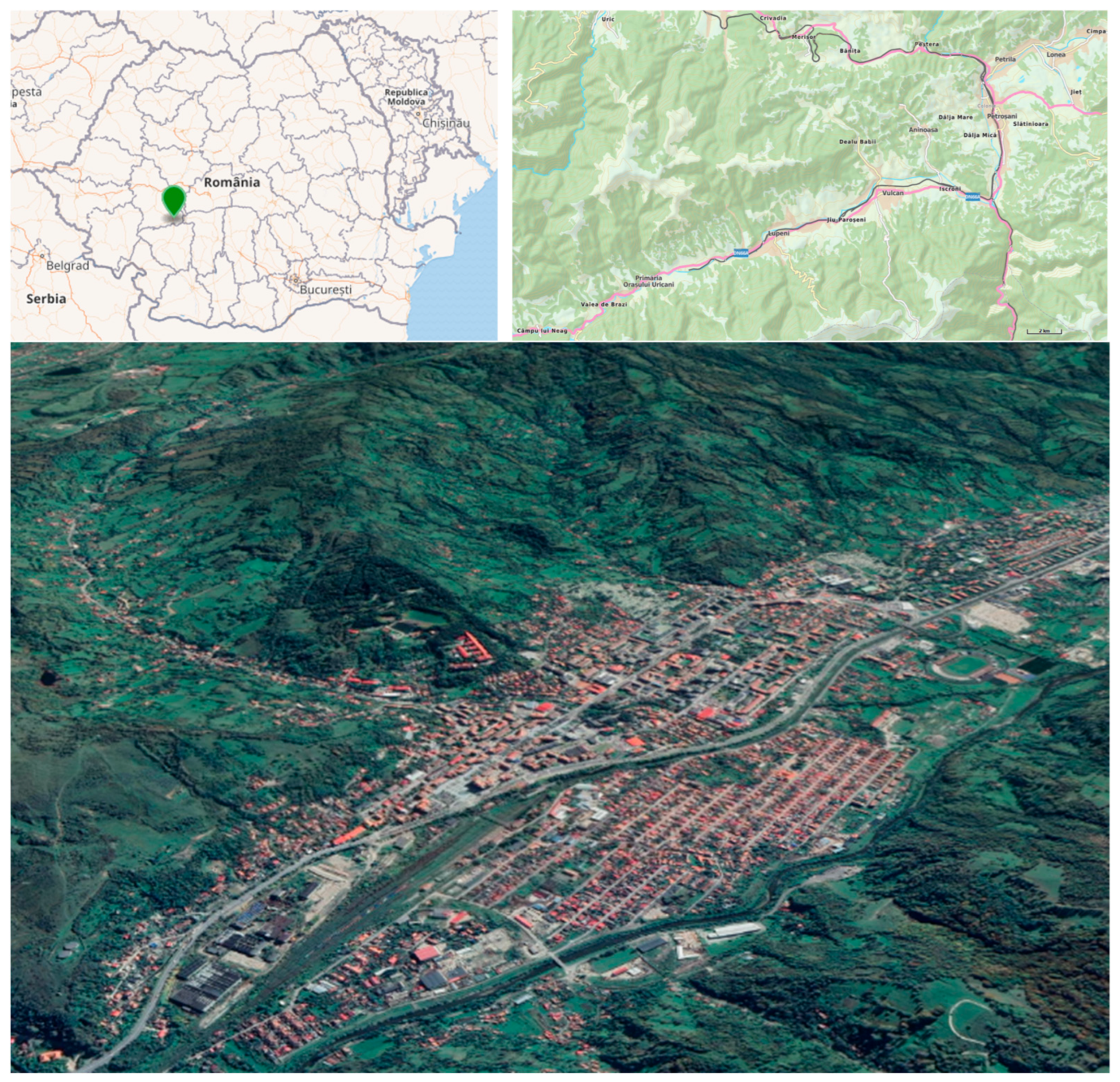
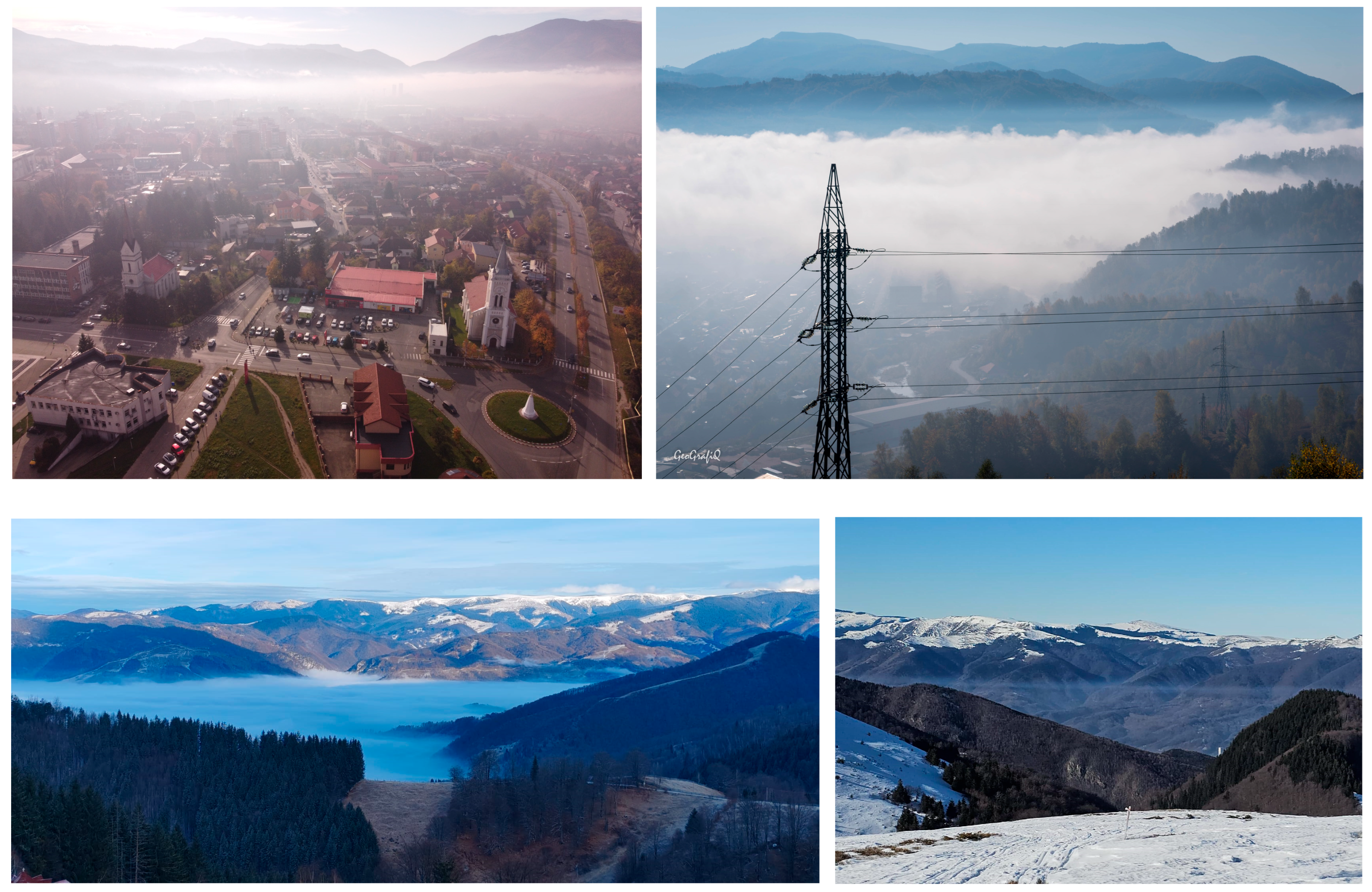
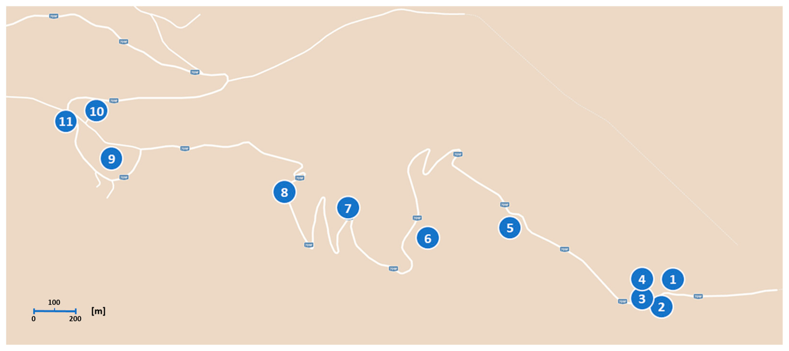
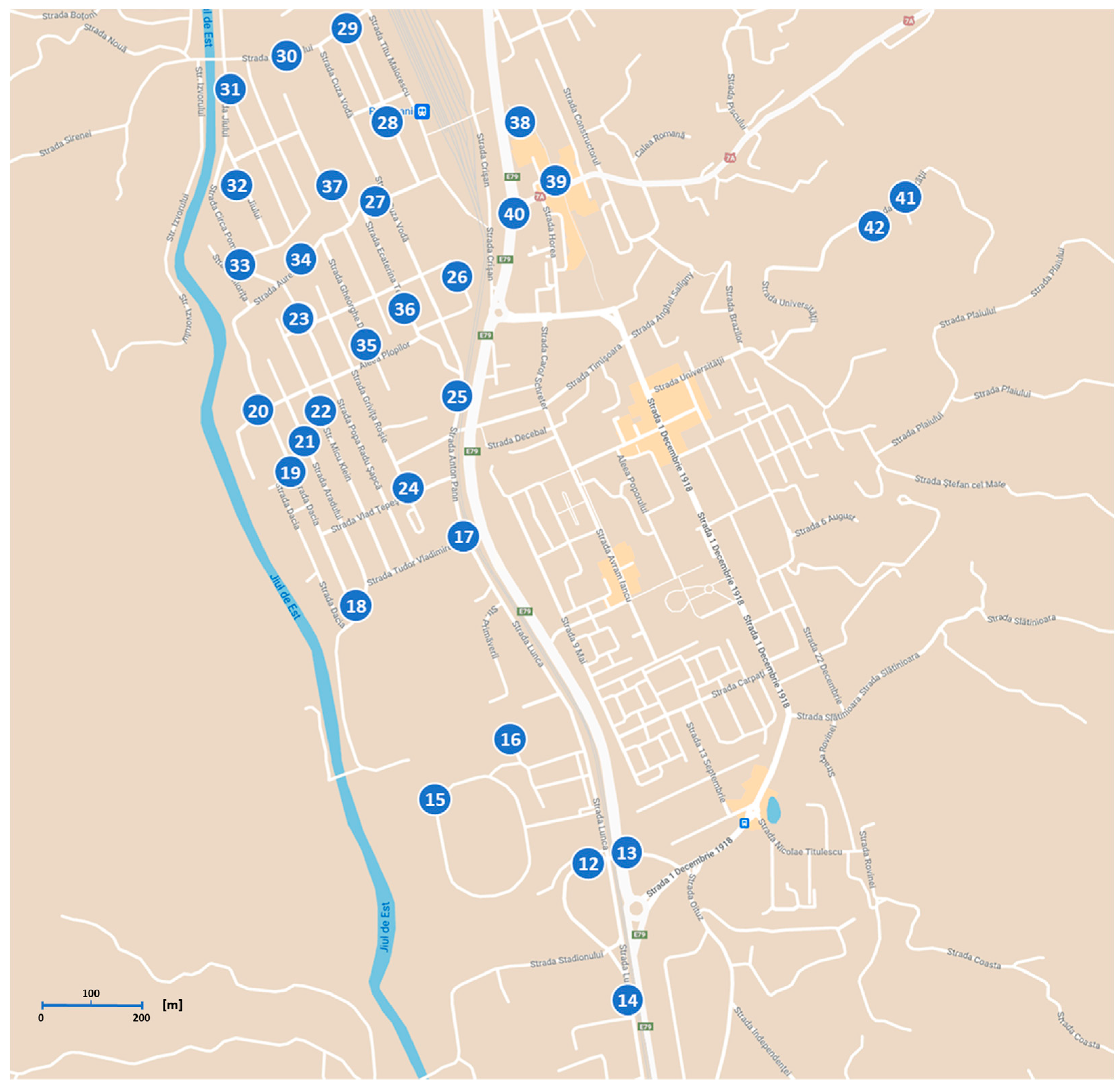

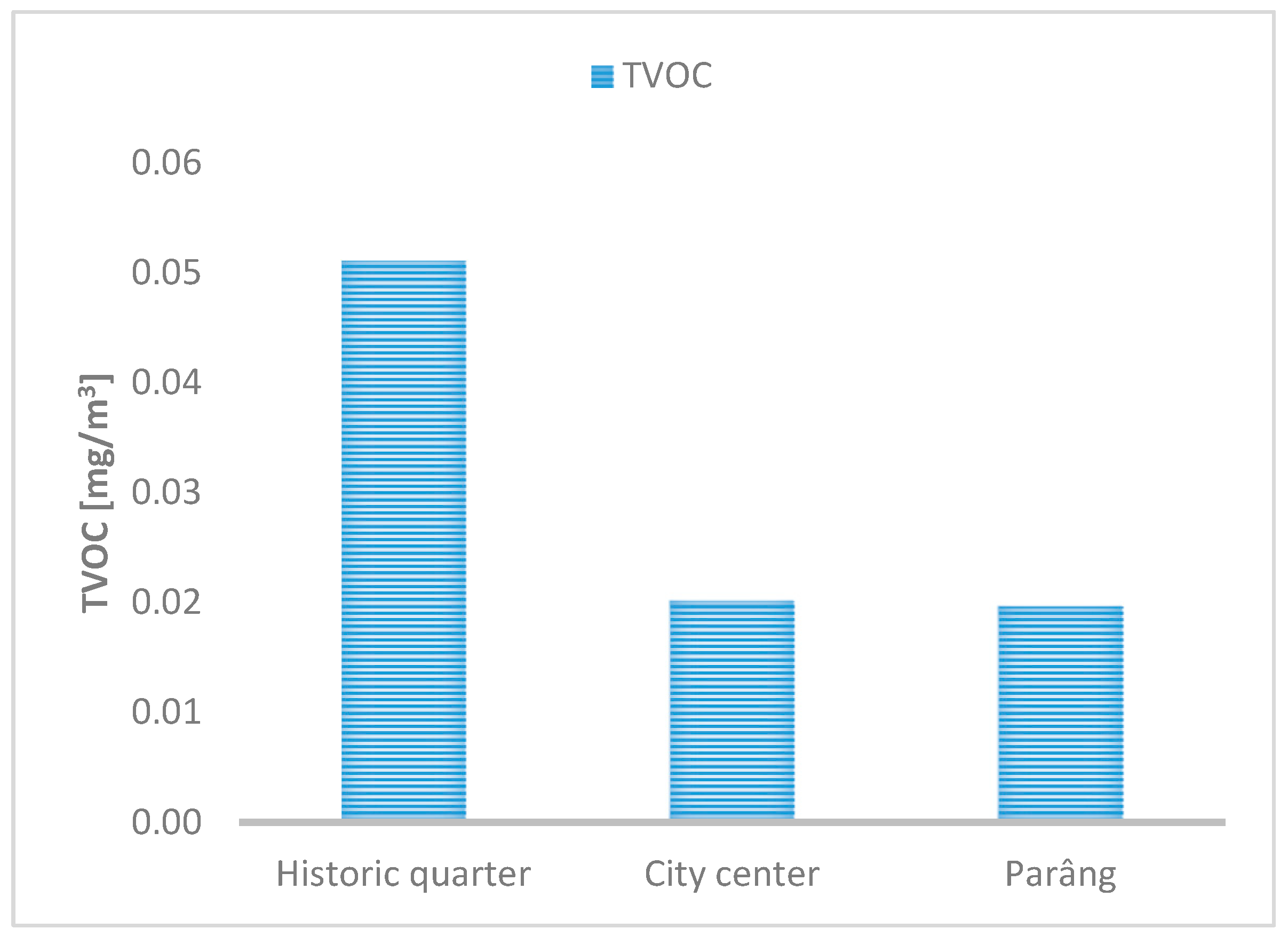

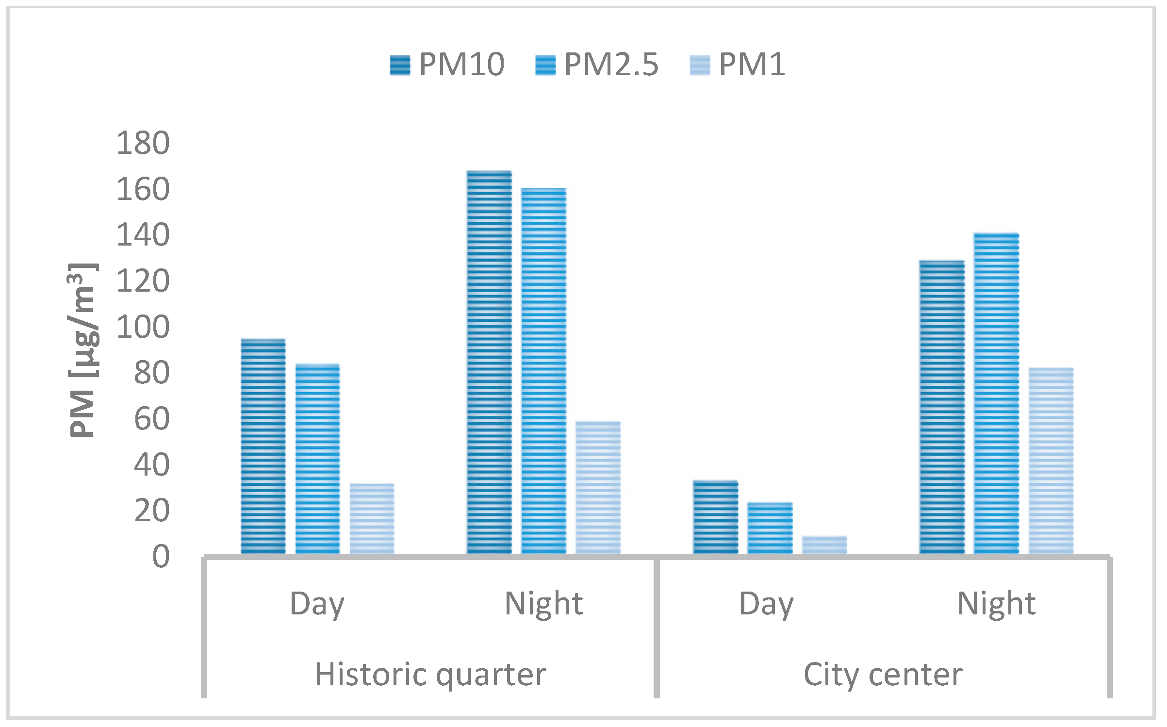
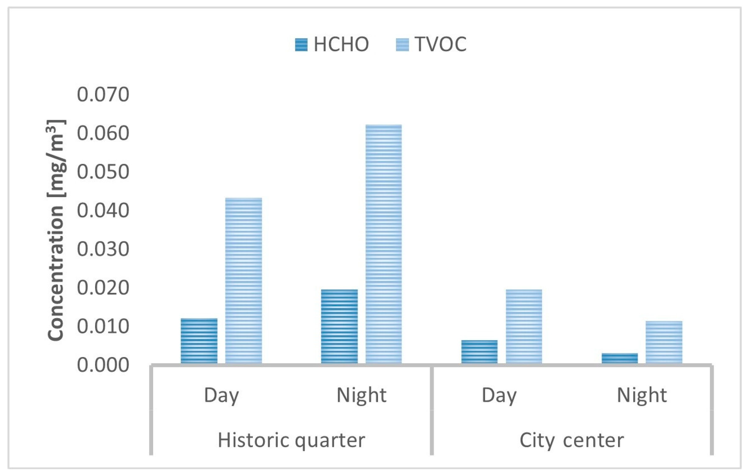

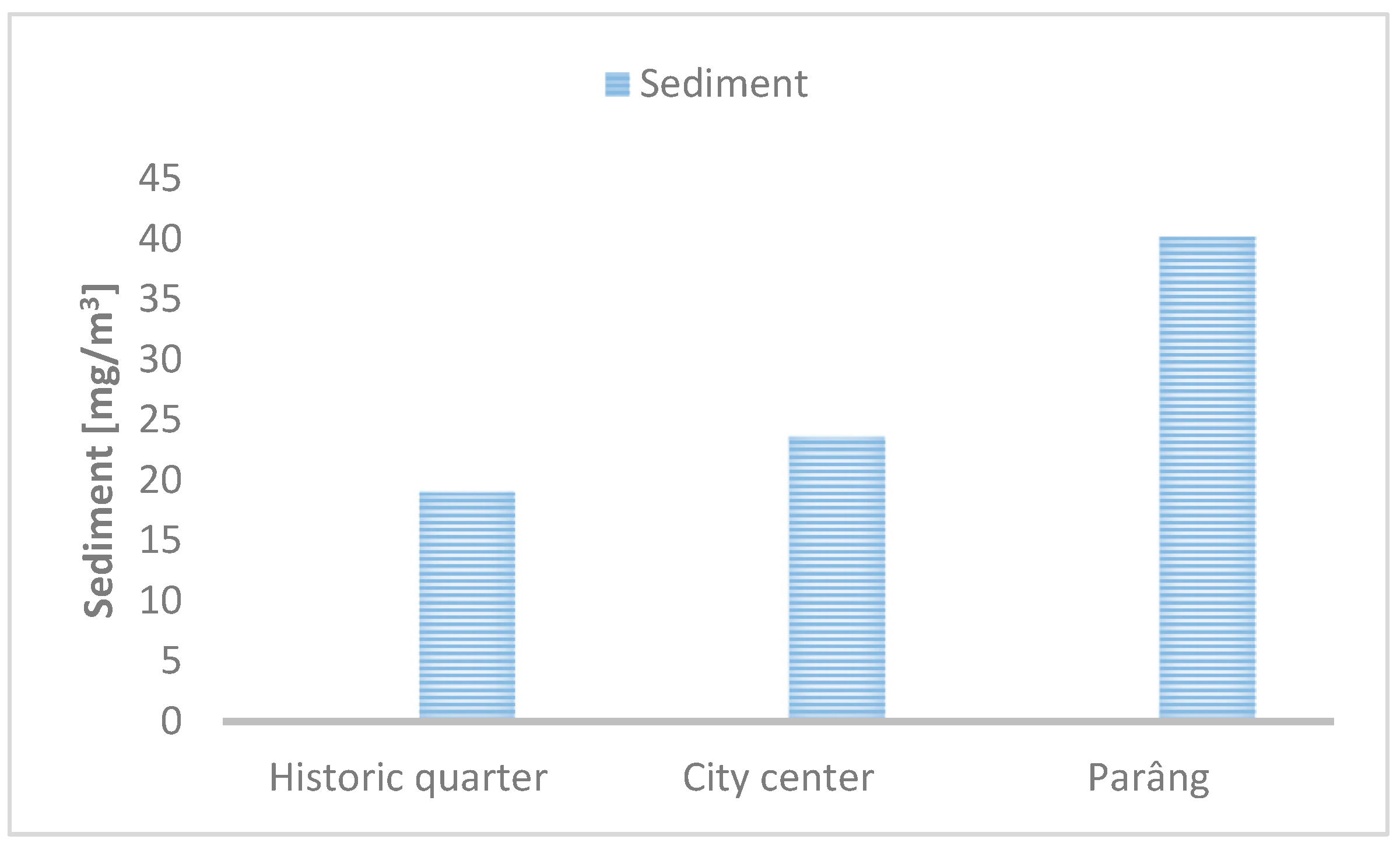
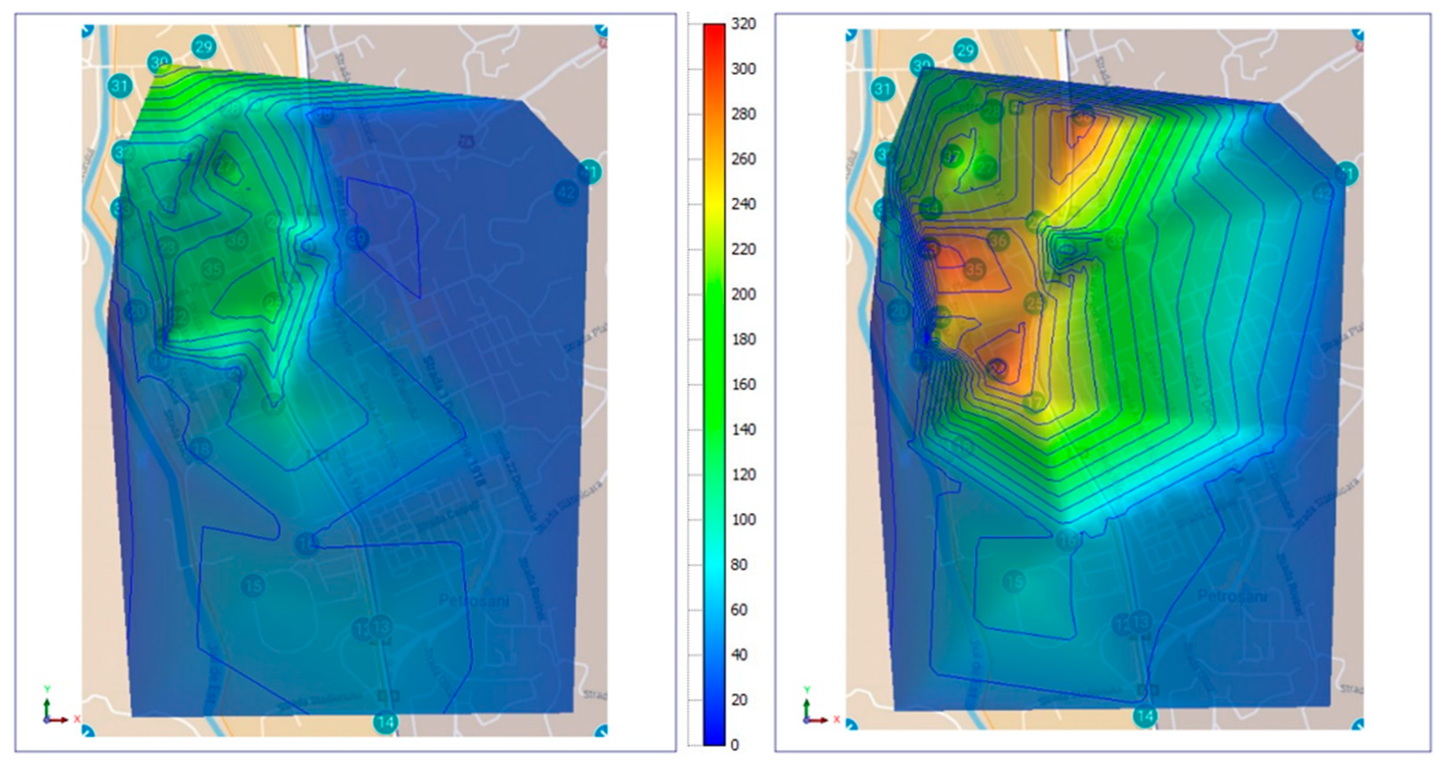
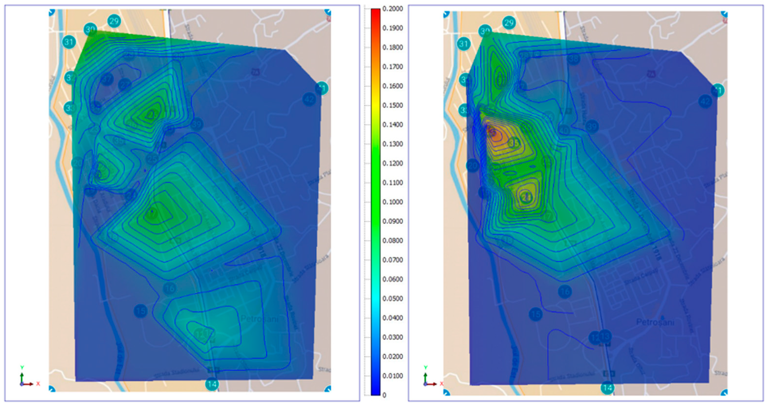
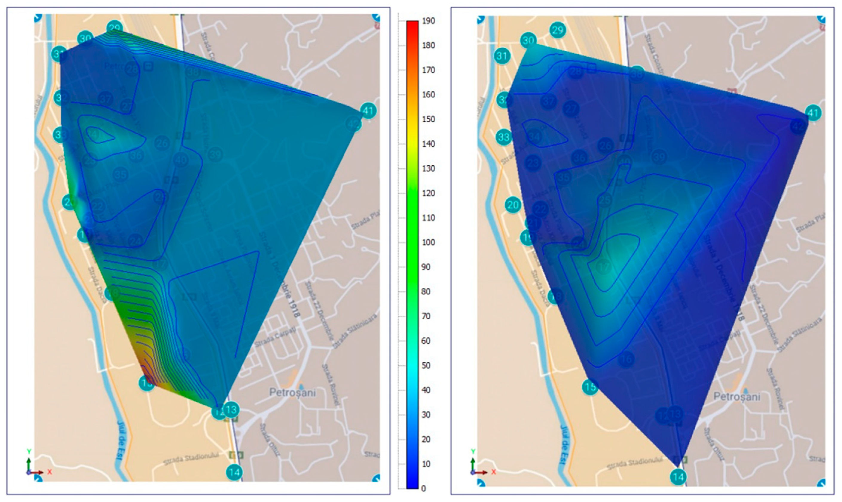

Disclaimer/Publisher’s Note: The statements, opinions and data contained in all publications are solely those of the individual author(s) and contributor(s) and not of MDPI and/or the editor(s). MDPI and/or the editor(s) disclaim responsibility for any injury to people or property resulting from any ideas, methods, instructions or products referred to in the content. |
© 2025 by the authors. Licensee MDPI, Basel, Switzerland. This article is an open access article distributed under the terms and conditions of the Creative Commons Attribution (CC BY) license (https://creativecommons.org/licenses/by/4.0/).