
The Impact of Heat Waves on Diurnal Variability and Spatial Structure of Atmospheric and Surface Urban Heat Islands in Kraków, Poland


Abstract
1. Introduction
2. Study Area
3. Data and Methods
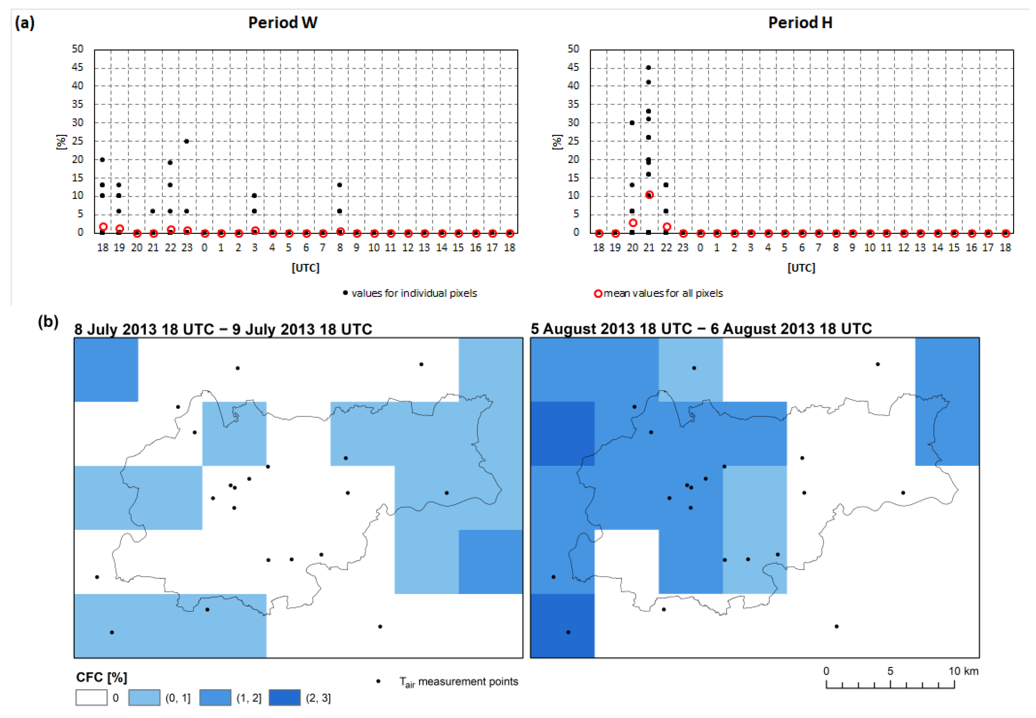
3.1. Study Periods
3.2. Vertical Zones and LCZ Classes
3.3. Data Sources
3.3.1. Air Temperature Measurements
3.3.2. Satellite Images
3.3.3. Land Surface Temperature Retrieval
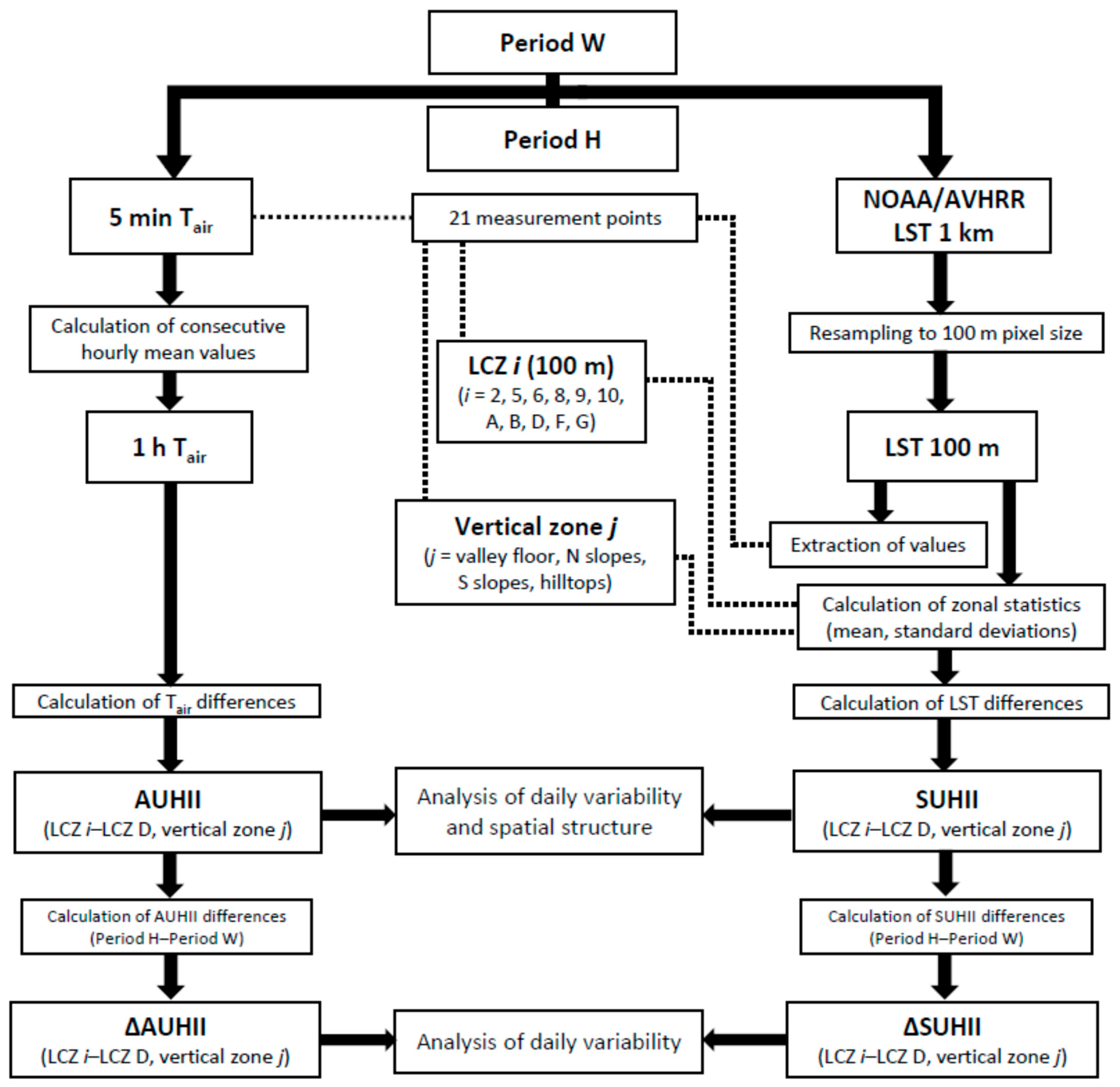
3.4. Methods for AUHI and SUHI Analysis
- AUHII and SUHII compatible in terms of location and time, i.e., at the Tair measurement points and the approximate acquisition times of satellite images;
- AUHII at individual Tair measurement points in a 3 h interval;
- SUHII at the approximate acquisition times of the NOAA/AVHRR satellite images for individual LCZ classes, separately for each vertical zone.
4. Results
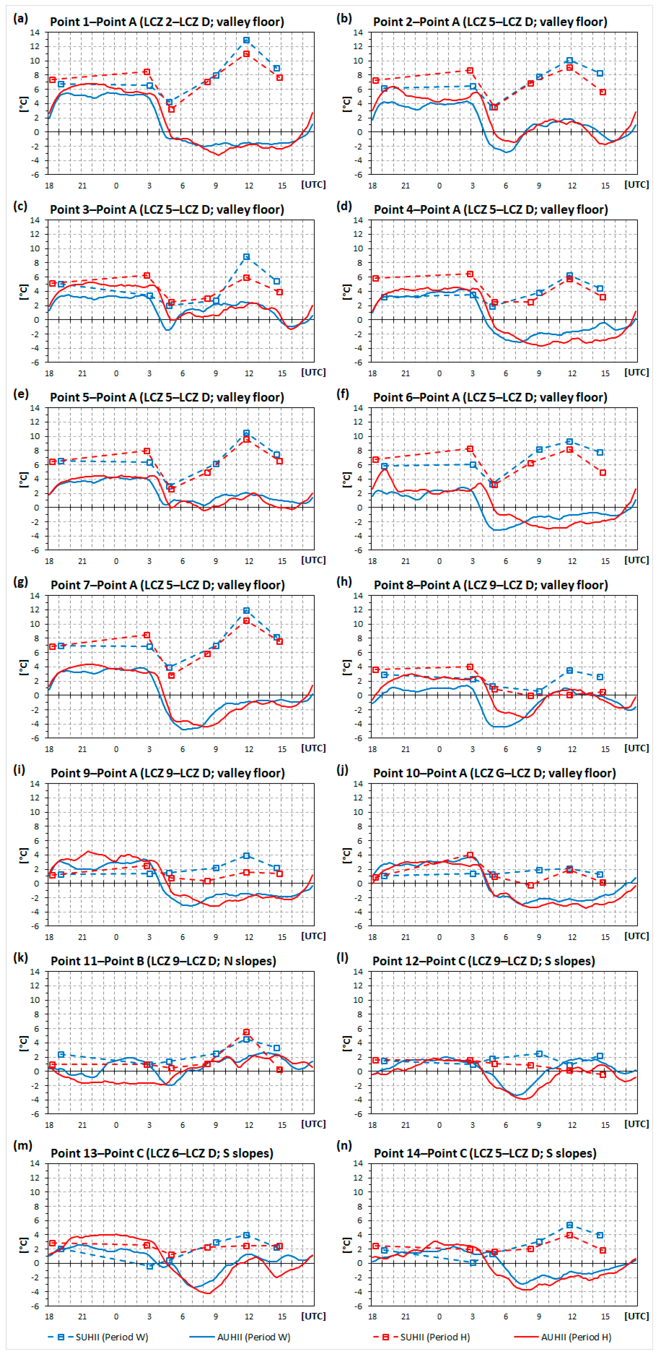
4.1. Analysis of AUHII and SUHII Daily Variability and Spatial Structure
4.2. Analysis of ΔAUHII and ΔSUHII Daily Variability
5. Discussion
6. Summary and Conclusions
Author Contributions
Funding
Institutional Review Board Statement
Informed Consent Statement
Data Availability Statement
Acknowledgments
Conflicts of Interest
Abbreviations
| UHI | Urban Heat Island |
| AUHI | Atmospheric Urban Heat Island |
| AUHII | Atmospheric Urban Heat Island Intensity |
| SUHI | Surface Urban Heat Island |
| SUHII | Surface Urban Heat Island Intensity |
| AUCI | Atmospheric Urban Cold Island |
| RMUHI | Relief-modified Urban Heat Island |
| UCL | Urban Canopy Layer |
| Tair | Air Temperature |
| LST | Land Surface Temperature |
| HW | Heat Wave |
| LCZ | Local Climate Zone |
| TIR | Thermal Infrared |
| NDVI | Normalized Difference Vegetation Index |
| AOD | Aerosol Optical Depth |
| PM | Particulate Matter |
Appendix A


| LCZ Class 1 | All Vertical Zones | Valley Floor | N Slopes | S Slopes | Hilltops | |
|---|---|---|---|---|---|---|
| Share [%] of LCZ Class | ||||||
| LCZ 2 (compact mid-rise) |  | 0.3 | 0.9 | - | - | - |
| LCZ 5 (open mid-rise) |  | 7.4 | 14.4 | 6.4 | 6.4 | - |
| LCZ 6 (open low-rise) |  | 3.2 | 3.8 | 1.5 | 8.9 | 0.1 |
| LCZ 8 (large low-rise) |  | 4.3 | 10.8 | 1.7 | 1.8 | - |
| LCZ 9 (sparsely built) |  | 24.7 | 20.1 | 17.4 | 40.4 | 27.0 |
| LCZ 10 (heavy industry) |  | 0.7 | 1.3 | 1.1 | - | - |
| LCZ A (dense trees) |  | 4.6 | 3.0 | 1.7 | 3.4 | 10.4 |
| LCZ B (scattered trees) |  | 5.2 | 6.6 | 0.9 | 7.7 | 5.8 |
| LCZ D (low plants) |  | 41.0 | 30.2 | 49.0 | 29.9 | 54.8 |
| LCZ F (bare soil or sand) |  | 8.3 | 7.9 | 20.2 | 1.4 | 1.9 |
| LCZ G (water) |  | 0.3 | 1.0 | - | - | - |
| LCZ Class Difference | Days Difference (7 August 2013–20 June 2013) | Days Difference (13 August 2015–12 July 2015) | ||||||
|---|---|---|---|---|---|---|---|---|
| Landsat LST Original 100 m | Landsat LST Upscaled to 1 km and Resampled to 100 m | Landsat LST Original 100 m | Landsat LST Upscaled to 1 km and Resampled to 100 m | |||||
| ΔSUHII [°C] | ΔSUHII [°C] | ΔSUHII [°C] | ΔSUHII [°C] | |||||
| µ | Σ | µ | σ | µ | σ | µ | σ | |
| LCZ 2–LCZ D | −3.3 | 1.5 | −3.1 | 0.2 | −1.9 | 0.6 | −1.5 | 0.1 |
| LCZ 5–LCZ D | −2.5 | 1.8 | −2.3 | 0.6 | −1.3 | 0.8 | −1.1 | 0.5 |
| LCZ 6–LCZ D | −2.0 | 1.6 | −1.7 | 0.7 | −1.6 | 0.9 | −1.2 | 0.7 |
| LCZ 8–LCZ D | −2.2 | 2.5 | −1.8 | 1.0 | −1.9 | 1.1 | −1.4 | 0.7 |
| LCZ 9–LCZ D | −1.5 | 1.7 | −1.2 | 0.8 | −1.2 | 1.2 | −0.9 | 0.8 |
| LCZ 10–LCZ D | −2.3 | 2.6 | −2.1 | 0.7 | −2.1 | 0.7 | −1.7 | 0.4 |
| LCZ A–LCZ D | −1.8 | 1.7 | −1.4 | 0.9 | −0.1 | 1.2 | −0.3 | 0.8 |
| LCZ B–LCZ D | −1.3 | 1.8 | −1.0 | 0.8 | −0.4 | 1.2 | −0.4 | 0.8 |
| LCZ F–LCZ D | −1.0 | 3.0 | −0.9 | 1.5 | −1.4 | 1.8 | −1.1 | 1.0 |
| LCZ G–LCZ D | −2.6 | 2.5 | −1.6 | 0.6 | 0.2 | 1.0 | −0.3 | 0.6 |
| Period | Vertical Zone | Tair Point | LCZ Class | Hour Interval [UTC] | |||||||||||||||
|---|---|---|---|---|---|---|---|---|---|---|---|---|---|---|---|---|---|---|---|
| 18–21 | 21–0 | 0–3 | 3–6 | 6–9 | 9–12 | 12–15 | 15–18 | ||||||||||||
| Tair [°C] | |||||||||||||||||||
| µ | σ | µ | σ | µ | σ | µ | σ | µ | σ | µ | σ | µ | σ | µ | σ | ||||
| W | Valley floor | 1 | LCZ 2 | 22.3 | 1.2 | 18.7 | 0.8 | 16.2 | 0.6 | 16.8 | 1.7 | 22.8 | 1.1 | 25.0 | 0.5 | 26.3 | 0.2 | 26.1 | 0.4 |
| 2 | LCZ 5 | 21.3 | 1.6 | 17.1 | 0.7 | 15.1 | 0.4 | 15.7 | 1.4 | 23.6 | 2.8 | 28.0 | 0.9 | 28.7 | 0.4 | 26.3 | 0.6 | ||
| 3 | LCZ 5 | 20.6 | 1.6 | 16.7 | 0.9 | 14.3 | 0.5 | 16.3 | 2.7 | 25.9 | 1.5 | 28.9 | 0.6 | 29.5 | 0.6 | 26.4 | 0.8 | ||
| 4 | LCZ 5 | 20.5 | 1.5 | 17.0 | 0.8 | 15.0 | 0.4 | 15.9 | 1.5 | 21.7 | 1.6 | 24.8 | 0.5 | 26.7 | 0.6 | 26.0 | 1.0 | ||
| 5 | LCZ 5 | 20.8 | 1.5 | 17.4 | 0.8 | 15.1 | 0.6 | 17.5 | 2.7 | 25.2 | 1.2 | 28.4 | 0.6 | 29.4 | 0.1 | 27.7 | 1.1 | ||
| 6 | LCZ 5 | 19.7 | 2.1 | 15.3 | 0.7 | 13.5 | 0.4 | 14.6 | 1.8 | 22.3 | 1.9 | 25.4 | 0.5 | 27.1 | 0.3 | 26.3 | 0.6 | ||
| 7 | LCZ 5 | 20.5 | 1.4 | 16.9 | 0.8 | 14.7 | 0.5 | 14.8 | 0.9 | 20.3 | 1.9 | 25.4 | 0.8 | 27.1 | 0.3 | 26.2 | 1.0 | ||
| 8 | LCZ 9 | 18.0 | 1.4 | 14.3 | 0.9 | 12.1 | 0.4 | 13.3 | 1.8 | 21.3 | 2.3 | 26.9 | 1.1 | 28.1 | 0.1 | 25.6 | 1.7 | ||
| 9 | LCZ 9 | 20.1 | 1.9 | 15.9 | 0.6 | 14.0 | 0.4 | 15.5 | 1.6 | 21.8 | 1.8 | 25.1 | 0.5 | 26.3 | 0.1 | 25.5 | 0.7 | ||
| 10 | LCZ G | 20.0 | 1.6 | 16.3 | 0.8 | 14.3 | 0.3 | 16.3 | 1.5 | 22.0 | 1.1 | 24.4 | 0.4 | 25.7 | 0.4 | 26.3 | 0.4 | ||
| A | LCZ D | 17.6 | 2.1 | 13.5 | 1.0 | 11.0 | 0.6 | 16.0 | 3.5 | 24.5 | 1.3 | 26.7 | 0.5 | 27.9 | 0.2 | 26.9 | 1.2 | ||
| N Slopes | 11 | LCZ 9 | 19.5 | 1.7 | 15.9 | 0.7 | 13.9 | 0.6 | 15.9 | 2.7 | 24.2 | 1.5 | 27.6 | 0.6 | 29.6 | 0.2 | 27.0 | 1.1 | |
| B | LCZ D | 19.5 | 1.3 | 15.9 | 1.5 | 12.2 | 0.5 | 16.9 | 3.3 | 23.8 | 1.0 | 26.1 | 0.6 | 27.2 | 0.1 | 26.1 | 1.1 | ||
| S Slopes | 12 | LCZ 9 | 19.1 | 1.8 | 15.6 | 0.7 | 13.5 | 0.6 | 15.0 | 1.7 | 21.0 | 1.8 | 26.7 | 1.2 | 28.7 | 0.2 | 26.1 | 1.3 | |
| 13 | LCZ 6 | 20.6 | 1.9 | 16.1 | 1.0 | 13.6 | 0.5 | 15.1 | 2.2 | 20.9 | 1.4 | 25.9 | 1.4 | 27.8 | 0.1 | 26.7 | 1.1 | ||
| 14 | LCZ 5 | 19.6 | 2.0 | 15.6 | 0.6 | 13.8 | 0.4 | 16.3 | 2.3 | 21.5 | 0.9 | 24.3 | 0.6 | 25.8 | 0.3 | 25.6 | 0.6 | ||
| C | LCZ D | 18.6 | 2.4 | 14.1 | 0.7 | 11.8 | 0.3 | 15.2 | 2.7 | 23.7 | 1.4 | 26.2 | 0.5 | 27.1 | 0.3 | 25.9 | 1.0 | ||
| Hilltops | D | LCZ D | 17.1 | 2.2 | 14.2 | 1.5 | 11.4 | 0.4 | 15.1 | 3.5 | 24.1 | 1.2 | 27.1 | 0.6 | 28.0 | 0.1 | 26.2 | 1.3 | |
| E | LCZ D | 20.7 | 0.9 | 18.9 | 0.4 | 16.1 | 0.8 | 17.6 | 2.0 | 23.5 | 0.6 | 25.4 | 0.6 | 26.7 | 0.2 | 26.0 | 0.9 | ||
| F | LCZ 9 | 20.6 | 0.7 | 17.8 | 0.7 | 15.2 | 0.4 | 15.8 | 0.7 | 20.4 | 1.5 | 25.5 | 1.7 | 27.9 | 0.4 | 25.2 | 1.3 | ||
| G | LCZ 9 | 19.6 | 0.4 | 18.5 | 0.4 | 16.6 | 0.6 | 18.8 | 0.8 | 21.6 | 1.0 | 23.7 | 0.4 | 24.6 | 0.2 | 23.8 | 0.7 | ||
| H | Valley floor | 1 | LCZ 2 | 26.6 | 1.0 | 23.6 | 0.8 | 20.9 | 0.6 | 20.0 | 0.9 | 25.6 | 1.7 | 30.7 | 1.3 | 33.0 | 0.2 | 31.9 | 0.8 |
| 2 | LCZ 5 | 26.7 | 1.4 | 21.8 | 0.9 | 19.7 | 0.3 | 20.3 | 0.7 | 26.9 | 3.1 | 34.6 | 0.9 | 35.1 | 0.9 | 32.2 | 0.9 | ||
| 3 | LCZ 5 | 25.3 | 1.3 | 22.0 | 0.8 | 19.9 | 0.5 | 20.2 | 1.4 | 28.1 | 2.3 | 34.6 | 1.3 | 36.8 | 0.3 | 32.2 | 1.6 | ||
| 4 | LCZ 5 | 24.6 | 1.2 | 21.3 | 0.6 | 19.6 | 0.4 | 19.4 | 0.9 | 24.7 | 1.8 | 29.9 | 1.1 | 32.2 | 0.2 | 30.9 | 1.1 | ||
| 5 | LCZ 5 | 24.6 | 1.4 | 21.4 | 0.7 | 19.5 | 0.5 | 20.1 | 1.7 | 27.6 | 2.0 | 34.1 | 1.3 | 36.0 | 0.5 | 32.9 | 1.6 | ||
| 6 | LCZ 5 | 24.9 | 2.7 | 19.3 | 0.8 | 17.5 | 0.3 | 19.3 | 1.6 | 25.6 | 1.8 | 30.4 | 0.9 | 32.9 | 0.4 | 32.0 | 0.9 | ||
| 7 | LCZ 5 | 24.5 | 1.3 | 21.1 | 0.9 | 18.7 | 0.6 | 17.8 | 0.6 | 23.4 | 2.1 | 30.7 | 1.7 | 34.0 | 0.3 | 31.6 | 1.4 | ||
| 8 | LCZ 9 | 22.7 | 1.1 | 19.6 | 0.9 | 17.5 | 0.5 | 18.4 | 1.3 | 24.8 | 2.4 | 33.3 | 1.6 | 35.2 | 0.3 | 31.1 | 2.2 | ||
| 9 | LCZ 9 | 24.3 | 1.6 | 20.9 | 1.0 | 18.8 | 0.6 | 18.8 | 1.4 | 25.0 | 1.8 | 30.7 | 1.2 | 33.2 | 0.3 | 31.2 | 1.3 | ||
| 10 | LCZ G | 23.1 | 1.3 | 19.9 | 0.7 | 17.9 | 0.6 | 18.3 | 1.6 | 24.8 | 1.7 | 30.2 | 0.9 | 32.0 | 0.3 | 30.6 | 1.5 | ||
| A | LCZ D | 21.2 | 2.2 | 17.0 | 0.7 | 15.2 | 0.4 | 18.0 | 3.3 | 27.4 | 2.4 | 33.2 | 0.9 | 35.1 | 0.4 | 32.5 | 2.3 | ||
| N Slopes | 11 | LCZ 9 | 23.0 | 1.6 | 19.8 | 0.6 | 17.7 | 0.5 | 18.5 | 1.8 | 26.6 | 2.4 | 33.2 | 1.1 | 35.8 | 0.3 | 32.2 | 2.0 | |
| B | LCZ D | 23.6 | 0.9 | 21.3 | 0.7 | 19.4 | 0.5 | 19.8 | 1.3 | 25.9 | 1.9 | 31.8 | 1.3 | 33.8 | 0.3 | 30.9 | 1.6 | ||
| S Slopes | 12 | LCZ 9 | 22.8 | 1.3 | 19.5 | 0.7 | 17.2 | 0.5 | 17.2 | 1.1 | 23.7 | 2.4 | 31.9 | 1.7 | 34.9 | 0.5 | 31.2 | 2.7 | |
| 13 | LCZ 6 | 25.5 | 0.7 | 22.3 | 1.2 | 19.4 | 0.7 | 18.7 | 0.8 | 23.7 | 1.9 | 31.4 | 2.1 | 34.1 | 0.9 | 31.4 | 1.3 | ||
| 14 | LCZ 5 | 23.8 | 1.5 | 20.5 | 0.7 | 18.3 | 0.5 | 18.1 | 1.0 | 23.9 | 2.1 | 30.2 | 1.1 | 32.5 | 0.3 | 31.1 | 1.4 | ||
| C | LCZ D | 22.9 | 1.6 | 18.4 | 1.3 | 15.7 | 0.4 | 18.0 | 2.5 | 27.1 | 2.6 | 32.8 | 0.8 | 34.5 | 0.4 | 31.8 | 2.1 | ||
| Hilltops | D | LCZ D | 20.4 | 1.7 | 16.8 | 0.6 | 15.7 | 0.2 | 18.4 | 2.1 | 26.2 | 2.0 | 31.9 | 1.4 | 34.2 | 0.1 | 30.5 | 2.3 | |
| E | LCZ D | 25.1 | 0.7 | 22.2 | 0.8 | 20.0 | 0.4 | 20.2 | 1.0 | 25.6 | 1.6 | 31.1 | 1.4 | 33.1 | 0.4 | 30.5 | 1.5 | ||
| F | LCZ 9 | 24.4 | 0.7 | 21.8 | 0.8 | 19.5 | 0.7 | 18.7 | 0.6 | 23.7 | 2.0 | 31.6 | 2.7 | 35.4 | 0.6 | 30.8 | 2.2 | ||
| G | LCZ 9 | 24.2 | 0.7 | 22.3 | 0.4 | 20.7 | 0.5 | 20.7 | 0.9 | 25.5 | 1.8 | 30.4 | 0.7 | 31.3 | 0.2 | 29.3 | 1.1 | ||
| Period | Vertical Zone | LCZ Class | Timestamp [Hour UTC] | |||||||||||
|---|---|---|---|---|---|---|---|---|---|---|---|---|---|---|
| 19 | 3 | 5 | 9 | 12 | 15 | |||||||||
| LST [°C] | ||||||||||||||
| µ | σ | µ | σ | µ | σ | µ | σ | µ | σ | µ | Σ | |||
| W | Valley floor | LCZ 2 | 22.4 | 0.2 | 16.1 | 0.6 | 18.6 | 0.3 | 33.0 | 0.9 | 41.0 | 1.4 | 34.4 | 0.8 |
| LCZ 5 | 21.0 | 1.4 | 14.3 | 1.3 | 17.1 | 0.9 | 30.9 | 1.5 | 38.2 | 2.0 | 32.1 | 1.4 | ||
| LCZ 6 | 18.4 | 1.6 | 12.2 | 1.5 | 16.0 | 0.7 | 28.9 | 1.5 | 34.9 | 2.3 | 29.3 | 2.0 | ||
| LCZ 8 | 18.7 | 1.8 | 12.2 | 1.5 | 16.4 | 0.9 | 29.7 | 1.3 | 36.2 | 2.1 | 30.5 | 1.9 | ||
| LCZ 9 | 17.2 | 1.1 | 11.0 | 1.0 | 15.5 | 0.7 | 27.8 | 1.3 | 32.7 | 1.9 | 27.9 | 1.4 | ||
| LCZ 10 | 19.5 | 1.3 | 13.6 | 1.2 | 17.0 | 1.4 | 30.4 | 1.8 | 38.2 | 2.9 | 32.3 | 2.2 | ||
| LCZ A | 16.9 | 0.8 | 10.7 | 0.5 | 15.1 | 0.6 | 27.0 | 1.3 | 31.2 | 1.5 | 26.5 | 1.0 | ||
| LCZ B | 17.1 | 1.1 | 11.1 | 1.3 | 15.3 | 0.9 | 27.5 | 1.6 | 31.7 | 2.0 | 27.3 | 1.7 | ||
| LCZ D | 16.5 | 0.8 | 10.6 | 1.1 | 15.4 | 0.7 | 27.2 | 1.1 | 31.6 | 1.7 | 27.0 | 1.3 | ||
| LCZ F | 17.0 | 0.9 | 11.0 | 1.0 | 16.0 | 0.5 | 29.6 | 1.7 | 35.1 | 2.4 | 29.5 | 2.0 | ||
| LCZ G | 17.3 | 1.4 | 11.2 | 1.3 | 15.9 | 0.5 | 27.7 | 1.5 | 32.0 | 2.2 | 27.2 | 2.0 | ||
| N Slopes | LCZ 5 | 21.2 | 1.0 | 13.9 | 0.9 | 16.8 | 0.6 | 30.6 | 1.2 | 38.0 | 1.8 | 31.8 | 1.2 | |
| LCZ 6 | 18.5 | 1.5 | 12.3 | 1.2 | 15.9 | 0.7 | 28.4 | 1.3 | 33.7 | 2.4 | 29.3 | 1.6 | ||
| LCZ 8 | 19.5 | 1.8 | 12.6 | 1.3 | 16.4 | 0.9 | 30.1 | 1.4 | 36.5 | 2.4 | 31.0 | 1.7 | ||
| LCZ 9 | 18.1 | 1.3 | 11.8 | 1.0 | 15.7 | 0.6 | 27.7 | 1.4 | 33.1 | 2.5 | 28.2 | 1.6 | ||
| LCZ 10 | 20.7 | 1.3 | 14.0 | 1.1 | 17.9 | 0.6 | 30.8 | 1.3 | 40.8 | 2.6 | 33.5 | 1.4 | ||
| LCZ A | 17.2 | 0.9 | 11.7 | 1.0 | 15.0 | 0.6 | 26.1 | 1.4 | 30.0 | 1.1 | 25.8 | 0.7 | ||
| LCZ B | 17.3 | 0.8 | 11.8 | 0.4 | 14.8 | 0.6 | 26.1 | 1.3 | 30.4 | 0.9 | 25.9 | 0.8 | ||
| LCZ D | 17.1 | 0.9 | 11.2 | 0.9 | 15.3 | 0.7 | 27.0 | 0.9 | 31.5 | 1.3 | 27.1 | 1.0 | ||
| LCZ F | 18.3 | 0.8 | 12.6 | 0.8 | 16.3 | 0.6 | 29.4 | 1.7 | 35.2 | 1.9 | 30.0 | 1.5 | ||
| S Slopes | LCZ 5 | 18.7 | 1.2 | 12.0 | 1.1 | 15.7 | 0.7 | 29.9 | 0.9 | 35.7 | 1.5 | 30.1 | 1.2 | |
| LCZ 6 | 17.8 | 1.2 | 11.4 | 1.1 | 15.4 | 0.6 | 28.5 | 0.8 | 34.1 | 1.5 | 28.8 | 1.3 | ||
| LCZ 8 | 17.8 | 1.8 | 11.5 | 1.1 | 15.2 | 0.9 | 28.4 | 1.1 | 34.6 | 2.5 | 29.3 | 1.3 | ||
| LCZ 9 | 16.6 | 0.9 | 10.8 | 0.9 | 15.0 | 0.7 | 27.4 | 1.1 | 31.8 | 1.6 | 27.2 | 1.2 | ||
| LCZ A | 16.6 | 0.7 | 10.6 | 0.6 | 14.8 | 0.9 | 26.0 | 1.4 | 30.3 | 1.1 | 25.9 | 0.9 | ||
| LCZ B | 16.2 | 0.8 | 10.5 | 1.0 | 14.6 | 0.8 | 26.6 | 1.0 | 30.7 | 1.6 | 26.1 | 1.0 | ||
| LCZ D | 16.2 | 0.6 | 10.9 | 0.7 | 15.2 | 0.7 | 26.1 | 1.0 | 30.6 | 1.0 | 26.3 | 0.7 | ||
| LCZ F | 16.4 | 0.3 | 10.9 | 0.6 | 15.5 | 0.7 | 26.5 | 1.0 | 31.1 | 0.6 | 26.7 | 0.5 | ||
| Hilltops | LCZ 6 | 16.4 | 0.2 | 11.8 | 0.1 | 15.6 | 0.3 | 26.7 | 0.9 | 30.8 | 1.9 | 25.8 | 0.7 | |
| LCZ 9 | 16.2 | 0.8 | 11.2 | 0.7 | 15.3 | 0.5 | 26.2 | 0.8 | 30.8 | 1.0 | 26.1 | 0.9 | ||
| LCZ A | 16.9 | 0.9 | 11.9 | 0.9 | 15.2 | 0.6 | 25.1 | 0.9 | 29.4 | 0.9 | 25.3 | 0.6 | ||
| LCZ B | 16.1 | 0.6 | 10.8 | 0.6 | 14.8 | 0.6 | 25.8 | 0.8 | 29.8 | 0.7 | 25.4 | 0.6 | ||
| LCZ D | 16.6 | 0.7 | 11.6 | 0.8 | 15.4 | 0.5 | 26.0 | 0.9 | 30.7 | 0.8 | 26.2 | 0.8 | ||
| LCZ F | 17.7 | 0.8 | 12.4 | 0.8 | 16.0 | 0.7 | 27.5 | 1.1 | 32.5 | 1.7 | 28.1 | 1.3 | ||
| H | Valley floor | LCZ 2 | 28.0 | 0.3 | 21.3 | 0.1 | 21.7 | 0.5 | 38.4 | 0.7 | 47.1 | 1.1 | 39.1 | 0.9 |
| LCZ 5 | 26.4 | 0.9 | 19.5 | 1.2 | 21.1 | 0.6 | 36.1 | 1.2 | 44.2 | 1.9 | 37.3 | 1.5 | ||
| LCZ 6 | 23.9 | 2.1 | 17.0 | 1.9 | 19.7 | 1.0 | 34.0 | 1.8 | 41.5 | 2.5 | 34.8 | 2.1 | ||
| LCZ 8 | 24.3 | 1.7 | 17.3 | 1.7 | 20.1 | 1.2 | 35.3 | 1.3 | 43.1 | 1.7 | 36.0 | 1.5 | ||
| LCZ 9 | 22.5 | 1.4 | 15.8 | 1.2 | 19.3 | 0.8 | 32.8 | 1.4 | 39.9 | 1.9 | 33.6 | 1.4 | ||
| LCZ 10 | 25.1 | 1.4 | 18.4 | 0.9 | 21.1 | 0.5 | 38.1 | 1.6 | 46.2 | 2.7 | 37.7 | 1.6 | ||
| LCZ A | 21.8 | 0.7 | 14.8 | 0.9 | 18.4 | 0.6 | 31.4 | 1.5 | 38.4 | 1.4 | 32.7 | 1.1 | ||
| LCZ B | 22.4 | 1.7 | 16.1 | 1.4 | 19.2 | 1.0 | 32.1 | 1.9 | 39.1 | 2.5 | 33.1 | 1.7 | ||
| LCZ D | 21.6 | 1.1 | 14.8 | 1.3 | 19.0 | 0.9 | 32.5 | 1.4 | 39.2 | 2.0 | 33.1 | 1.3 | ||
| LCZ F | 22.7 | 0.9 | 15.7 | 1.3 | 20.1 | 0.9 | 35.2 | 1.3 | 42.5 | 2.3 | 35.0 | 1.5 | ||
| LCZ G | 22.6 | 1.5 | 16.2 | 1.7 | 19.9 | 0.7 | 32.5 | 1.3 | 39.3 | 1.9 | 33.5 | 1.5 | ||
| N Slopes | LCZ 5 | 25.5 | 0.8 | 18.9 | 0.8 | 21.0 | 0.3 | 35.6 | 1.0 | 44.1 | 1.0 | 37.2 | 1.0 | |
| LCZ 6 | 23.0 | 1.0 | 16.9 | 0.7 | 20.0 | 0.4 | 33.4 | 1.2 | 40.9 | 2.7 | 34.2 | 2.1 | ||
| LCZ 8 | 24.0 | 1.3 | 17.9 | 1.2 | 20.7 | 0.5 | 35.4 | 1.1 | 43.0 | 1.4 | 36.6 | 1.5 | ||
| LCZ 9 | 22.8 | 1.0 | 16.7 | 1.1 | 19.9 | 0.7 | 33.0 | 1.5 | 40.4 | 2.1 | 34.2 | 1.8 | ||
| LCZ 10 | 25.1 | 0.9 | 18.4 | 0.7 | 20.9 | 0.3 | 38.0 | 1.2 | 46.0 | 1.5 | 38.3 | 1.8 | ||
| LCZ A | 22.4 | 1.0 | 15.9 | 0.9 | 19.1 | 0.6 | 30.2 | 1.3 | 37.0 | 2.4 | 31.1 | 1.5 | ||
| LCZ B | 22.5 | 1.2 | 15.7 | 0.6 | 19.0 | 0.4 | 29.4 | 1.5 | 36.9 | 2.0 | 31.6 | 1.5 | ||
| LCZ D | 22.0 | 1.0 | 16.0 | 1.3 | 19.7 | 0.7 | 32.7 | 1.4 | 39.6 | 2.1 | 33.6 | 1.5 | ||
| LCZ F | 23.0 | 0.5 | 17.4 | 0.8 | 20.6 | 0.6 | 35.0 | 1.0 | 43.2 | 1.4 | 35.8 | 0.9 | ||
| S Slopes | LCZ 5 | 25.3 | 1.1 | 17.9 | 0.9 | 20.4 | 0.6 | 35.4 | 1.0 | 42.6 | 1.2 | 35.8 | 1.3 | |
| LCZ 6 | 24.1 | 1.5 | 17.0 | 1.2 | 19.6 | 0.5 | 34.5 | 1.1 | 41.2 | 1.5 | 34.6 | 1.5 | ||
| LCZ 8 | 24.6 | 1.8 | 17.4 | 1.4 | 19.7 | 0.9 | 35.0 | 1.4 | 42.2 | 1.9 | 35.5 | 1.9 | ||
| LCZ 9 | 22.0 | 1.3 | 15.3 | 1.1 | 18.7 | 0.9 | 32.8 | 1.2 | 39.0 | 1.6 | 32.8 | 1.4 | ||
| LCZ A | 21.7 | 0.8 | 15.2 | 0.8 | 18.2 | 0.7 | 30.7 | 1.1 | 36.7 | 1.3 | 31.3 | 0.8 | ||
| LCZ B | 21.4 | 1.2 | 14.8 | 0.9 | 18.1 | 1.0 | 31.8 | 1.2 | 37.8 | 1.8 | 31.8 | 1.4 | ||
| LCZ D | 21.3 | 0.8 | 15.2 | 0.9 | 18.7 | 0.9 | 32.5 | 1.6 | 38.5 | 1.8 | 32.6 | 1.4 | ||
| LCZ F | 20.9 | 0.5 | 14.7 | 0.6 | 17.8 | 0.9 | 31.8 | 1.2 | 38.1 | 1.5 | 32.0 | 1.3 | ||
| Hilltops | LCZ 6 | 22.5 | 0.6 | 16.7 | 0.7 | 19.0 | 0.7 | 33.0 | 0.4 | 38.3 | 0.2 | 32.2 | 0.5 | |
| LCZ 9 | 21.1 | 0.9 | 15.7 | 0.9 | 18.5 | 0.7 | 31.4 | 1.0 | 37.2 | 1.5 | 31.4 | 1.1 | ||
| LCZ A | 21.8 | 1.0 | 16.4 | 0.8 | 18.6 | 0.7 | 30.0 | 0.9 | 35.9 | 1.7 | 30.7 | 1.4 | ||
| LCZ B | 20.9 | 0.7 | 15.2 | 0.6 | 18.4 | 0.6 | 30.4 | 0.7 | 36.1 | 1.1 | 30.7 | 0.8 | ||
| LCZ D | 21.3 | 0.8 | 16.1 | 0.9 | 19.2 | 0.7 | 31.7 | 1.2 | 38.2 | 1.7 | 32.4 | 1.4 | ||
| LCZ F | 22.6 | 0.7 | 17.0 | 1.0 | 20.0 | 0.6 | 33.6 | 1.0 | 40.8 | 1.4 | 34.4 | 0.9 | ||
References
- Arnfield, A.J. Two decades of urban climate research: A review of turbulence, exchanges of energy and water, and the urban heat island. Int. J. Climatol. 2003, 23, 1–26. [Google Scholar] [CrossRef]
- Stewart, I.D. A systematic review and scientific critique of methodology in modern urban heat island literature. Int. J. Climatol. 2011, 31, 200–217. [Google Scholar] [CrossRef]
- Kong, J.; Zhao, Y.; Carmeliet, J.; Lei, C. Urban Heat Island and Its Interaction with Heatwaves: A Review of Studies on Mesoscale. Sustainability 2021, 13, 10923. [Google Scholar] [CrossRef]
- IPCC. Climate Change 2021: The Physical Science Basis. Contribution of Working Group I to the Sixth Assessment Report of the Intergovernmental Panel on Climate Change; Cambridge University Press: Cambridge, UK, 2023. [Google Scholar] [CrossRef]
- Roth, M.; Oke, T.R.; Emery, W.J. Satellite-derived urban heat islands from three coastal cities and the utilization of such data in urban climatology. Int. J. Remote Sens. 1989, 10, 1699–1720. [Google Scholar] [CrossRef]
- Voogt, J.A.; Oke, T.R. Thermal remote sensing of urban climates. Remote Sens. Environ. 2003, 86, 370–384. [Google Scholar] [CrossRef]
- Oke, T.R. The distinction between canopy and boundary-layer urban heat islands. Atmosphere 1976, 14, 268–277. [Google Scholar] [CrossRef]
- Grimmond, C.S.B. Progress in measuring and observing the urban atmosphere. Theor. Appl. Climatol. 2006, 84, 3–22. [Google Scholar] [CrossRef]
- Parlow, E.; Vogt, R.; Feigenwinter, C. The urban heat island of Basel—Seen from different perspectives. Erde 2014, 145, 96–110. [Google Scholar] [CrossRef]
- Stewart, I.D.; Oke, T.R. Local Climate Zones for Urban Temperature Studies. Bull. Am. Meteorol. Soc. 2012, 93, 1879–1900. [Google Scholar] [CrossRef]
- Sobrino, J.A.; Oltra-Carrió, R.; Sòria, G.; Bianchi, R.; Paganini, M. Impact of spatial resolution and satellite overpass time on evaluation of the surface urban heat island effects. Remote Sens. Environ. 2012, 117, 50–56. [Google Scholar] [CrossRef]
- Amorim, M.C.C.T.; Dubreuil, V.; Amorim, A.T. Day and night surface and atmospheric heat islands in a continental and temperate tropical environment. Urban Clim. 2021, 38, 100918. [Google Scholar] [CrossRef]
- Oke, T.R. The energetic basis of the urban heat island. Quart. J. R. Meteorol. Soc. 1982, 108, 1–24. [Google Scholar] [CrossRef]
- Zhou, D.; Xiao, J.; Bonafoni, S.; Berger, C.; Deilami, K.; Zhou, Y.; Frolking, S.; Yao, R.; Qiao, Z.; Sobrino, J.A. Satellite Remote Sensing of Surface Urban Heat Islands: Progress, Challenges, and Perspectives. Remote Sens. 2019, 11, 48. [Google Scholar] [CrossRef]
- Szymanowski, M. Interactions between thermal advection in frontal zones and the urban heat island of Wrocław, Poland. Theor. Appl. Climatol. 2005, 82, 207–224. [Google Scholar] [CrossRef]
- Graham, E. The Urban Heat Island of Dublin City During the Summer Months. Ir. Geogr. 1993, 26, 45–57. [Google Scholar] [CrossRef]
- Saaroni, H.; Ziv, B. Estimating the Urban Heat Island Contribution to Urban and Rural Air Temperature Differences over Complex Terrain: Application to an Arid City. J. Appl. Meteorol. Climatol. 2010, 49, 2159–2166. [Google Scholar] [CrossRef]
- Ketterer, C.; Matzarakis, A. Human-Biometeorological Assessment of the Urban Heat Island in a City with Complex Topography—The Case of Stuttgart, Germany. Urban Clim. 2014, 10, 573–584. [Google Scholar] [CrossRef]
- Ketterer, C.; Matzarakis, A. Comparison of Different Methods for the Assessment of the Urban Heat Island in Stuttgart, Germany. Int. J. Biometeorol. 2015, 59, 1299–1309. [Google Scholar] [CrossRef]
- Li, G.; Zhang, X.; Mirzaei, P.A.; Zhang, J.; Zhao, Z. Urban Heat Island Effect of a Typical Valley City in China: Responds to the Global Warming and Rapid Urbanization. Sustain. Cities Soc. 2018, 38, 736–745. [Google Scholar] [CrossRef]
- Heinl, M.; Hammerle, A.; Tappeiner, U.; Leitinger, G. Determinants of Urban–Rural Land Surface Temperature Differences—A Landscape Scale Perspective. Landsc. Urban Plan. 2015, 134, 33–42. [Google Scholar] [CrossRef]
- Equere, V.; Mirzaei, P.A.; Riffat, S.; Wang, Y. Integration of Topological Aspect of City Terrains to Predict the Spatial Distribution of Urban Heat Island Using GIS and ANN. Sustain. Cities Soc. 2021, 69, 102825. [Google Scholar] [CrossRef]
- Liao, D.; Zhu, H.; Jiang, P. Study of Urban Heat Island Index Methods for Urban Agglomerations (Hilly Terrain) in Chongqing. Theor. Appl. Climatol. 2021, 143, 279–289. [Google Scholar] [CrossRef]
- Badaro-Saliba, N.; Adjizian-Gerard, J.; Zaarour, R.; Najjar, G. LCZ Scheme for Assessing Urban Heat Island Intensity in a Complex Urban Area (Beirut, Lebanon). Urban Clim. 2021, 37, 100846. [Google Scholar] [CrossRef]
- Bokwa, A.; Hajto, M.J.; Walawender, J.P.; Szymanowski, M. Influence of Diversified Relief on the Urban Heat Island in the City of Kraków, Poland. Theor. Appl. Climatol. 2015, 122, 365–382. [Google Scholar] [CrossRef]
- Walawender, J.P.; Szymanowski, M.; Hajto, M.J.; Bokwa, A. Land Surface Temperature Patterns in the Urban Agglomeration of Krakow (Poland) Derived from Landsat-7/ETM+ Data. Pure Appl. Geophys. 2014, 171, 913–940. [Google Scholar] [CrossRef]
- Schwarz, N.; Schlink, U.; Franck, U.; Großmann, K. Relationship of Land Surface and Air Temperatures and Its Implications for Quantifying Urban Heat Island Indicators—An Application for the City of Leipzig (Germany). Ecol. Indic. 2012, 18, 693–704. [Google Scholar] [CrossRef]
- Sobrino, J.A.; Oltra-Carrió, R.; Sòria, G.; Jiménez-Muñoz, J.C.; Franch, B.; Hidalgo, V.; Mattar, C.; Julien, Y.; Cuenca, J.; Romaguera, M.; et al. Evaluation of the Surface Urban Heat Island Effect in the City of Madrid by Thermal Remote Sensing. Int. J. Remote Sens. 2013, 34, 3177–3192. [Google Scholar] [CrossRef]
- Fung, W.Y.; Lam, K.S.; Nichol, J.; Wong, M.S. Derivation of Nighttime Urban Air Temperatures Using a Satellite Thermal Image. J. Appl. Meteor. Climatol. 2009, 48, 863–872. [Google Scholar] [CrossRef]
- Nichol, J.E.; To, P.H. Temporal Characteristics of Thermal Satellite Images for Urban Heat Stress and Heat Island Mapping. ISPRS J. Photogramm. Remote Sens. 2012, 74, 153–162. [Google Scholar] [CrossRef]
- Kourtidis, K.; Georgoulias, A.K.; Rapsomanikis, S.; Amiridis, V.; Keramitsoglou, I.; Hooyberghs, H.; Maiheu, B.; Melas, D. A Study of the Hourly Variability of the Urban Heat Island Effect in the Greater Athens Area During Summer. Sci. Total Environ. 2015, 517, 162–177. [Google Scholar] [CrossRef]
- Gallo, K.P.; McNab, A.L.; Karl, T.R.; Brown, J.F.; Hood, J.J.; Tarpley, J.D. The Use of NOAA AVHRR Data for Assessment of the Urban Heat Island Effect. J. Appl. Meteor. Climatol. 1993, 32, 899–908. [Google Scholar] [CrossRef]
- Holderness, T.; Barr, S.; Dawson, R.; Hall, J. An Evaluation of Thermal Earth Observation for Characterizing Urban Heatwave Event Dynamics Using the Urban Heat Island Intensity Metric. Int. J. Remote Sens. 2013, 34, 864–884. [Google Scholar] [CrossRef]
- Anniballe, R.; Bonafoni, S.; Pichierri, M. Spatial and Temporal Trends of the Surface and Air Heat Island Over Milan Using MODIS Data. Remote Sens. Environ. 2014, 150, 163–171. [Google Scholar] [CrossRef]
- Cheval, S.; Dumitrescu, A.; Bell, A. The Urban Heat Island of Bucharest During the Extreme High Temperatures of July 2007. Theor. Appl. Climatol. 2009, 97, 391–401. [Google Scholar] [CrossRef]
- Sun, H.; Chen, Y.; Zhan, W. Comparing Surface- and Canopy-Layer Urban Heat Islands Over Beijing Using MODIS Data. Int. J. Remote Sens. 2015, 36, 5448–5465. [Google Scholar] [CrossRef]
- Tomlinson, C.J.; Chapman, L.; Thornes, J.E.; Baker, C.J. Derivation of Birmingham’s Summer Surface Urban Heat Island from MODIS Satellite Images. Int. J. Climatol. 2012, 32, 214–224. [Google Scholar] [CrossRef]
- Venter, Z.S.; Chakraborty, T.; Lee, X. Crowdsourced Air Temperatures Contrast Satellite Measures of the Urban Heat Island and Its Mechanisms. Sci. Adv. 2021, 7, eabb9569. [Google Scholar] [CrossRef]
- Mohan, M.; Kikegawa, Y.; Gurjar, B.R.; Bhati, S.; Kolli, N.R. Assessment of Urban Heat Island Effect for Different Land Use–Land Cover from Micrometeorological Measurements and Remote Sensing Data for Megacity Delhi. Theor. Appl. Climatol. 2013, 112, 647–658. [Google Scholar] [CrossRef]
- Cui, Y.Y.; de Foy, B. Seasonal Variations of the Urban Heat Island at the Surface and the Near-Surface and Reductions Due to Urban Vegetation in Mexico City. J. Appl. Meteor. Climatol. 2012, 51, 855–868. [Google Scholar] [CrossRef]
- Caselles, V.; López García, M.J.; Meliá, J.; Pérez Cueva, A.J. Analysis of the Heat-Island Effect of the City of Valencia, Spain, Through Air Temperature Transects and NOAA Satellite Data. Theor. Appl. Climatol. 1991, 43, 195–203. [Google Scholar] [CrossRef]
- Azevedo, J.A.; Chapman, L.; Muller, C.L. Quantifying the Daytime and Night-Time Urban Heat Island in Birmingham, UK: A Comparison of Satellite-Derived Land Surface Temperature and High-Resolution Air Temperature Observations. Remote Sens. 2016, 8, 153. [Google Scholar] [CrossRef]
- Zhou, B.; Lauwaet, D.; Hooyberghs, H.; Ridder, K.D.; Kropp, J.P.; Rybski, D. Assessing Seasonality in the Surface Urban Heat Island of London. J. Appl. Meteor. Climatol. 2016, 55, 493–505. [Google Scholar] [CrossRef]
- Dezső, Z.; Pongrácz, R.; Bartholy, J. Surface Urban Heat Island in Budapest During Heat Waves and Droughts—Comparing the Summers of 2003, 2007 and 2022. Urban Clim. 2024, 55, 101899. [Google Scholar] [CrossRef]
- Dousset, B.; Gourmelon, F.; Laaidi, K.; Zeghnoun, A.; Giraudet, E.; Bretin, P.; Mauri, E.; Vandentorren, S. Satellite Monitoring of Summer Heat Waves in the Paris Metropolitan Area. Int. J. Climatol. 2011, 31, 313–323. [Google Scholar] [CrossRef]
- García, D.H. Analysis of Urban Heat Island and Heat Waves Using Sentinel-3 Images: A Study of Andalusian Cities in Spain. Earth Syst. Environ. 2022, 6, 199–219. [Google Scholar] [CrossRef] [PubMed]
- Kabisch, N.; Remahne, F.; Ilsemann, C.; Fricke, L. The Urban Heat Island Under Extreme Heat Conditions: A Case Study of Hannover, Germany. Sci. Rep. 2023, 13, 23017. [Google Scholar] [CrossRef]
- Kong, J.; Zhao, Y.; Strebel, D.; Gao, K.; Carmeliet, J.; Lei, C. Understanding the Impact of Heatwave on Urban Heat in Greater Sydney: Temporal Surface Energy Budget Change with Land Types. Sci. Total Environ. 2023, 903, 166374. [Google Scholar] [CrossRef]
- Schwarz, N.; Lautenbach, S.; Seppelt, R. Exploring Indicators for Quantifying Surface Urban Heat Islands of European Cities with MODIS Land Surface Temperatures. Remote Sens. Environ. 2011, 115, 3175–3186. [Google Scholar] [CrossRef]
- Stewart, I.D.; Krayenhoff, E.S.; Voogt, J.A.; Lachapelle, J.A.; Allen, M.A.; Broadbent, A.M. Time Evolution of the Surface Urban Heat Island. Earth’s Future 2021, 9, e2021EF002178. [Google Scholar] [CrossRef]
- Wei, L.; Sobrino, J.A. Surface Urban Heat Island Analysis Based on Local Climate Zones Using ECOSTRESS and Landsat Data: A Case Study of Valencia City (Spain). Int. J. Appl. Earth Obs. Geoinf. 2024, 130, 103875. [Google Scholar] [CrossRef]
- Cheval, S.; Amihăesei, V.-A.; Chitu, Z.; Dumitrescu, A.; Falcescu, V.; Irașoc, A.; Micu, D.M.; Mihulet, E.; Ontel, I.; Paraschiv, M.-G.; et al. A systematic review of urban heat island and heat waves research (1991–2022). Clim. Risk Manag. 2024, 44, 100603. [Google Scholar] [CrossRef]
- Núñez-Peiró, M.; Sánchez, C.S.-G.; González, F.J.N. Hourly Evolution of Intra-Urban Temperature Variability Across the Local Climate Zones: The Case of Madrid. Urban Clim. 2021, 39, 100921. [Google Scholar] [CrossRef]
- Skarbit, N.; Stewart, I.D.; Unger, J.; Gál, T. Employing an Urban Meteorological Network to Monitor Air Temperature Conditions in the ‘Local Climate Zones’ of Szeged, Hungary. Int. J. Climatol. 2017, 37, 582–596. [Google Scholar] [CrossRef]
- Wibig, J. Heat Waves in Poland in the Period 1951–2015: Trends, Patterns and Driving Factors. Meteor. Hydrol. Water Manag. 2018, 6, 37–45. [Google Scholar] [CrossRef]
- Tomczyk, A.M.; Bednorz, E.; Półrolniczak, M.; Kolendowicz, L. Strong Heat and Cold Waves in Poland in Relation to the Large-Scale Atmospheric Circulation. Theor. Appl. Climatol. 2019, 137, 1909–1923. [Google Scholar] [CrossRef]
- Bokwa, A.; Geletič, J.; Lehnert, M.; Žuvela-Aloise, M.; Hollósi, B.; Gál, T.; Skarbit, N.; Dobrovolný, P.; Hajto, M.J.; Kielar, R.; et al. Heat Load Assessment in Central European Cities Using an Urban Climate Model and Observational Monitoring Data. Energy Build. 2019, 201, 53–69. [Google Scholar] [CrossRef]
- Walawender, J. Wykorzystanie danych satelitarnych LANDSAT i technik GIS w badaniach warunków termicznych miasta (na przykładzie Aglomeracji Krakowskiej) [Application of LANDSAT Satellite Data and GIS Techniques for Estimation of Thermal Conditions in Urban Area (Using an Example of Krakow Agglomeration)]. Pr. Geogr. 2009, 122, 81–98. Available online: https://ruj.uj.edu.pl/xmlui/handle/item/147548 (accessed on 30 January 2025).
- Hajto, M. Badanie czasowo-przestrzennej struktury warunków termicznych terenów miejskich i pozamiejskich na podstawie danych satelitarnych [Investigation of Temporal-Spatial Structure of Urban and Non-Urban Surfaces’ Thermal Conditions on the Basis of Satellite Data]. Pr. Geogr. 2009, 122, 71–79. [Google Scholar]
- Statistical Bulletin of the City of Kraków—4th Quarter 2023; Statistical Office in Kraków: Kraków, Poland, 2024. Available online: https://krakow.stat.gov.pl/en/current-studies/communiques/other-studies/statistical-bulletin-of-krakow-guarter-42023,1,69.html (accessed on 30 September 2024).
- Jarvis, A.; Reuter, H.I.; Nelson, A.; Guevara, E. Hole-Filled SRTM for the Globe Version 4. Available online: http://srtm.csi.cgiar.org (accessed on 30 January 2025).
- Lewińska, J.; Zgud, K. Wyspa ciepła na tle zespołów urbanistycznych Krakowa [Heat Island Versus Urban Complexes of Krakow]. Przegląd Geofiz. 1980, 25, 283–294. [Google Scholar]
- Bokwa, A. Wieloletnie Zmiany Struktury Mezoklimatu Miasta na Przykładzie Krakowa [Multi-Annual Changes of the Urban Mesoclimate Structure (Using an Example of Kraków)]; Institute of Geography and Spatial Management of the Jagiellonian University: Kraków, Poland, 2010; Available online: https://jbc.bj.uj.edu.pl/dlibra/publication/28455/edition/23007 (accessed on 30 January 2025).
- Hess, M. Klimat Krakowa [Climate of Kraków]. Folia Geogr. Ser. Geogr.-Phys. 1974, 8, 45–102. [Google Scholar]
- Godłowska, J. Wpływ Warunków Meteorologicznych na Jakość powietrza w Krakowie. Badania Porównawcze i Próba Podejścia Modelowego [Influence of Meteorological Conditions on Air Quality in Kraków. Comparative Research and an Attempt at a Model Approach]; IMGW-PIB: Warszawa, Poland, 2019; Available online: https://imgw.pl/wplyw-warunkow-meteorologicznych-na-jakosc-powietrza-w-krakowie/ (accessed on 30 January 2025).
- Walczewski, J.; Feleksy-Bielak, M. Diurnal Variation of Characteristic Sodar Echoes and the Diurnal Change of Atmospheric Stability. Atmos. Environ. 1988, 22, 1793–1800. [Google Scholar] [CrossRef]
- Bokwa, A. Influence of Air Temperature Inversions on the Air Pollution Dispersion Conditions in Krakow. Pr. Geogr. 2011, 126, 41–51. Available online: https://bibliotekanauki.pl/articles/634037 (accessed on 30 January 2025).
- Wojkowski, J. Promieniowanie słoneczne [Solar Radiation]. In Klimat Krakowa w XX Wieku; Matuszko, D., Ed.; Institute of Geography and Spatial Management of the Jagiellonian University: Kraków, Poland, 2007; pp. 55–74. [Google Scholar]
- Niedźwiedź, T. Kalendarz Typów Cyrkulacji Atmosfery dla Polski Południowej—Zbiór Komputerowy [Calendar of Air Circulation Types for Southern Poland—Computer File]; Uniwersytet Śląski, Katedra Klimatologii: Sosnowiec, Poland, 2024; Available online: https://us.edu.pl/instytut/inoz/kalendarz-typow-cyrkulacji/ (accessed on 30 September 2024).
- Stöckli, R.; Duguay–Tetzlaff, A.; Bojanowski, J.; Hollmann, R.; Fuchs, P.; Werscheck, M. CM SAF Cloud Fractional Cover Dataset from METEOSAT First and Second Generation—Edition 1 (COMET Ed. 1); Satellite Application Facility on Climate Monitoring: Offenbach, Germany, 2017. [Google Scholar] [CrossRef]
- Levy, R.; Hsu, C.; et al. MODIS Atmosphere L2 Aerosol Product; NASA MODIS Adaptive Processing System, Goddard Space Flight Center: Greenbelt, MD, USA. [CrossRef]
- Bartoszek, K.; Matuszko, D.; Soroka, J. Relationships Between Cloudiness, Aerosol Optical Thickness, and Sunshine Duration in Poland. Atmos. Res. 2020, 245, 105097. [Google Scholar] [CrossRef]
- Naz, B.S.; Kollet, S.; Franssen, H.-J.H.; Montzka, C.; Kurtz, W. A 3 km Spatially and Temporally Consistent European Daily Soil Moisture Reanalysis from 2000 to 2015. Sci. Data 2020, 7, 111. [Google Scholar] [CrossRef]
- Bechtel, B.; Alexander, P.J.; Böhner, J.; Ching, J.; Conrad, O.; Feddema, J.; Mills, G.; See, L.; Stewart, I. Mapping Local Climate Zones for a Worldwide Database of the Form and Function of Cities. ISPRS Int. J. Geo-Inf. 2015, 4, 199–219. [Google Scholar] [CrossRef]
- Ulivieri, C.; Castronuovo, M.M.; Francioni, R.; Cardillo, A. A Split Window Algorithm for Estimating Land Surface Temperature from Satellites. Adv. Space Res. 1994, 14, 59–65. [Google Scholar] [CrossRef]
- Coll, C.; Caselles, V. A Split-Window Algorithm for Land Surface Temperature from Advanced Very High Resolution Radiometer Data: Validation and Algorithm Comparison. J. Geophys. Res. Atmos. 1997, 102, 16697–16713. [Google Scholar] [CrossRef]
- Frey, C.M.; Kuenzer, C.; Dech, S. Assessment of Mono- and Split-Window Approaches for Time Series Processing of LST from AVHRR—A TIMELINE Round Robin. Remote Sens. 2017, 9, 72. [Google Scholar] [CrossRef]
- Vázquez, D.P.; Reyes, F.J.O.; Arboledas, L.A. A Comparative Study of Algorithms for Estimating Land Surface Temperature from AVHRR Data. Remote Sens. Environ. 1997, 62, 215–222. [Google Scholar] [CrossRef]
- Rigo, G.; Parlow, E.; Oesch, D. Validation of Satellite Observed Thermal Emission with In-Situ Measurements Over an Urban Surface. Remote Sens. Environ. 2006, 104, 201–210. [Google Scholar] [CrossRef]
- Sobrino, J.A.; Raissouni, N.; Li, Z.-L. A Comparative Study of Land Surface Emissivity Retrieval from NOAA Data. Remote Sens. Environ. 2001, 75, 256–266. [Google Scholar] [CrossRef]
- Sobrino, J.A.; Jimenez-Munoz, J.C.; Soria, G.; Romaguera, M.; Guanter, L.; Moreno, J.; Plaza, A.; Martinez, P. Land Surface Emissivity Retrieval from Different VNIR and TIR Sensors. IEEE Trans. Geosci. Remote Sens. 2008, 46, 316–327. [Google Scholar] [CrossRef]
- Sobrino, J.A.; Raissouni, N. Toward Remote Sensing Methods for Land Cover Dynamic Monitoring: Application to Morocco. Int. J. Remote Sens. 2000, 21, 353–366. [Google Scholar] [CrossRef]
- Pichierri, M.; Bonafoni, S.; Biondi, R. Satellite Air Temperature Estimation for Monitoring the Canopy Layer Heat Island of Milan. Remote Sens. Environ. 2012, 127, 130–138. [Google Scholar] [CrossRef]

| Period | Starting Date and Time | Ending Date and Time | Sunset Time | Sunrise Time |
|---|---|---|---|---|
| W | 8 July 2013 18 UTC | 9 July 2013 18 UTC | 18:50 UTC | 02:42 UTC |
| H | 5 August 2013 18 UTC | 6 August 2013 18 UTC | 18:16 UTC | 03:16 UTC |
| Period | Cloud Cover [%] | Air Temperature [°C] | Relative Humidity [%] | Wind Speed [m·s−1] | Wind Direction | |||
|---|---|---|---|---|---|---|---|---|
| Avg | Min | Max | Avg | Max | ||||
| W | 2.5 | 20.3 | 12.3 | 26.3 | 64 | 1.7 | 4.0 | NE |
| H | 3.0 | 24.7 | 17.0 | 32.9 | 58 | 2.2 | 4.0 | NE |
| Tair Measurement Point | Altitude [m a.s.l.] | Vertical Zone b | Land Use/Cover c | LCZ Class (% Shares) d | |
|---|---|---|---|---|---|
| Symbol a | Name | ||||
| 1 | Słowackiego Theatre | 215 | Valley floor | Compact built-up (with street canyons) | LCZ 2 (79%), LCZ 5 (16%), LCZ 8 (5%) |
| 2 | Krasińskiego St. | 204 | Valley floor | Compact built-up (with street canyons) | LCZ 5 (86%), LCZ 2 (14%) |
| 3 | Podwawelskie district | 203 | Valley floor | Blocks of flats | LCZ 5 (100%) |
| 4 | Szkolne district | 205 | Valley floor | Blocks of flats | LCZ 5 (94%), LCZ D (6%) |
| 5 | Bema St. | 208 | Valley floor | Residential built-up | LCZ 5 (54%), LCZ 6 (46%) |
| 6 | Błonia meadows | 203 | Valley floor | Urban green areas | LCZ 5 (93%), LCZ 2 (7%) |
| 7 | Botanical Garden | 206 | Valley floor | Urban green areas | LCZ 5 (97%), LCZ 6 (3%) |
| 8 | Malczewskiego St. | 222 | Valley floor | Urban green areas | LCZ 9 (90%), LCZ B (10%) |
| 9 | Wandy Bridge | 197 | Valley floor | Water bodies | LCZ 9 (91%), LCZ D (9%) |
| 10 | Przylasek Rusiecki | 190 | Valley floor | Water bodies | LCZ G (63%), LCZ D (37%) |
| 11 | Ojcowska St. | 245 | N slopes | Residential built-up | LCZ 9 (100%) |
| 12 | Czajna St. | 258 | S slopes | Residential built-up | LCZ 9 (100%) |
| 13 | Bojki St. | 252 | S slopes | Blocks of flats | LCZ 6 (64%), LCZ 5 (33%), LCZ 9 (3%) |
| 14 | Mała Góra St. | 231 | S slopes | Blocks of flats | LCZ 5 (94%), LCZ 6 (5%), LCZ 9 (1%) |
| A | Jeziorzany | 211 | Valley floor | Rural areas | LCZ D (100%) |
| B | Modlniczka | 258 | N slopes | Rural areas | LCZ D (93%), LCZ B (5%), LCZ A (3%) |
| C | Rzozów | 251 | S slopes | Rural areas | LCZ D (45%), LCZ B (23%), LCZ 9 (33%) |
| D | Garlica Murowana | 270 | N hilltops | Rural areas | LCZ D (100%) |
| E | Kocmyrzów | 299 | N hilltops | Rural areas | LCZ D (91%), LCZ F (9%) |
| F | Libertów | 314 | S hilltops | Rural areas | LCZ 9 (100%) |
| G | Chorągwica | 436 | S hilltops | Rural areas | LCZ 9 (94%), LCZ D (6%) |
| Period W | Period H | ||
|---|---|---|---|
| AVHRR Image Time Over the Study Area | Satellite | AVHRR Image Time Over the Study Area | Satellite |
| 8 July 2013 19:08 UTC | NOAA-16 | 5 August 2013 18:22 UTC | NOAA-16 |
| 9 July 2013 03:07 UTC | NOAA-18 | 6 August 2013 02:57 UTC | NOAA-18 |
| 9 July 2013 04:54 UTC | NOAA-15 | 6 August 2013 05:10 UTC | NOAA-15 |
| 9 July 2013 09:05 UTC | NOAA-16 | 6 August 2013 08:20 UTC | NOAA-16 |
| 9 July 2013 11:50 UTC | NOAA-19 | 6 August 2013 11:49 UTC | NOAA-19 |
| 9 July 2013 14:40 UTC | NOAA-15 | 6 August 2013 14:55 UTC | NOAA-15 |
| Vertical Zone | Difference of Tair Measurement Points (Urban–Rural) | LCZ Class Difference | Period H–Period W | |||||||||||
|---|---|---|---|---|---|---|---|---|---|---|---|---|---|---|
| Timestamp [Hour UTC] | Timestamp [Hour UTC] | |||||||||||||
| 19 | 3 | 5 | 9 | 12 | 15 | 19 | 3 | 5 | 9 | 12 | 15 | |||
| ΔAUHII [°C] | ΔSUHII [°C] | |||||||||||||
| Valley floor | Point 1–Point A | LCZ 2–LCZ D | −1.6 | 0.6 | 0.4 | −0.8 | −0.3 | −0.7 | 0.6 | 1.9 | −1.0 | −0.8 | −1.9 | −1.3 |
| Point 2–Point A | LCZ 5–LCZ D | −0.3 | 1.1 | 1.9 | −0.7 | −0.4 | −1.5 | 1.1 | 2.2 | 0.0 | −1.0 | −1.0 | −2.5 | |
| Point 3–Point A | LCZ 5–LCZ D | −0.6 | 1.6 | 1.4 | −1.8 | −0.4 | 0.3 | 0.1 | 2.8 | 0.4 | 0.3 | −2.9 | −1.6 | |
| Point 4–Point A | LCZ 5–LCZ D | −1.3 | 0.5 | 0.5 | −1.6 | −1.2 | −2.3 | 2.7 | 3.0 | 0.6 | −1.3 | −0.5 | −1.2 | |
| Point 5–Point A | LCZ 5–LCZ D | −1.0 | 0.3 | −0.5 | −1.8 | −0.6 | −1.1 | −0.1 | 1.7 | −0.5 | −1.2 | −0.9 | −0.9 | |
| Point 6–Point A | LCZ 5–LCZ D | 1.5 | 0.2 | 2.6 | −1.1 | −1.5 | −1.0 | 0.9 | 2.2 | −0.1 | −1.9 | −1.2 | −2.8 | |
| Point 7–Point A | LCZ 5–LCZ D | −1.2 | −0.2 | −0.1 | −2.3 | −0.6 | −0.6 | −0.2 | 1.6 | −1.2 | −1.2 | −1.4 | −0.6 | |
| Point 8–Point A | LCZ 9–LCZ D | −0.3 | 1.3 | 2.7 | −1.9 | −0.1 | −0.6 | 0.7 | 1.8 | −0.4 | −0.6 | −3.4 | −2.1 | |
| Point 9–Point A | LCZ 9–LCZ D | −0.9 | 0.1 | 0.6 | −1.4 | −0.6 | −0.3 | −0.2 | 1.2 | −0.8 | −1.9 | −2.4 | −0.8 | |
| Point 10–Point A | LCZ G–LCZ D | −2.1 | −1.3 | −0.5 | −1.1 | −0.8 | −1.0 | −0.2 | 2.6 | −0.3 | −2.1 | −0.2 | −1.2 | |
| N Slopes | Point 11–Point B | LCZ 9–LCZ D | 0.0 | −2.6 | 0.9 | −0.2 | −0.4 | −0.3 | −1.4 | 0.1 | −0.9 | −1.4 | 1.0 | −3.1 |
| S Slopes | Point 12–Point C | LCZ 9–LCZ D | −0.6 | 0.3 | −1.8 | −2.7 | −1.4 | −0.5 | 0.0 | 0.6 | −0.7 | −1.6 | −0.8 | −2.6 |
| Point 13–Point C | LCZ 6–LCZ D | −0.7 | 2.2 | −0.6 | −2.2 | −0.9 | −2.1 | 0.8 | 2.9 | 0.7 | −0.6 | −1.5 | 0.2 | |
| Point 14–Point C | LCZ 5–LCZ D | 0.1 | 1.0 | −2.8 | −1.8 | −0.7 | −0.5 | 0.6 | 1.9 | 0.2 | −1.0 | −1.4 | −2.1 | |
 | ||||||||||||||
| Vertical Zone | Difference of Tair Measurement Points (Urban–Rural) | LCZ Class Difference | Period H–Period W | |||||||
|---|---|---|---|---|---|---|---|---|---|---|
| Hour Interval [UTC] | ||||||||||
| 18–21 | 21–0 | 0–3 | 3–6 | 6–9 | 9–12 | 12–15 | 15–18 | |||
| ΔAUHII 1 [°C] | ||||||||||
| µ (σ) | µ (σ) | µ (σ) | µ (σ) | µ (σ) | µ (σ) | µ (σ) | µ (σ) | |||
| Valley floor | Point 1–Point A | LCZ 2–LCZ D | 0.8 (0.4) | 1.4 (0.4) | 0.5 (0.2) | 1.1 (0.9) | −0.1 (0.4) | −0.8 (0.5) | −0.4 (0.2) | 0.2 (0.8) |
| Point 2–Point A | LCZ 5–LCZ D | 1.8 (0.4) | 1.2 (0.6) | 0.5 (0.2) | 2.6 (0.9) | 0.4 (0.8) | 0.1 (0.5) | −0.7 (0.6) | 0.4 (0.8) | |
| Point 3–Point A | LCZ 5–LCZ D | 1.1 (0.4) | 1.9 (0.3) | 1.5 (0.2) | 2.0 (1.3) | −0.8 (0.3) | −0.8 (0.4) | 0.2 (0.4) | 0.3 (0.6) | |
| Point 4–Point A | LCZ 5–LCZ D | 0.5 (0.4) | 0.8 (0.3) | 0.4 (0.2) | 1.4 (0.7) | 0.0 (0.9) | −1.4 (0.3) | −1.6 (0.5) | −0.7 (1.0) | |
| Point 5–Point A | LCZ 5–LCZ D | 0.3 (0.2) | 0.5 (0.4) | 0.2 (0.1) | 0.6 (1.1) | −0.5 (0.3) | −0.8 (0.4) | −0.5 (0.5) | −0.3 (0.7) | |
| Point 6–Point A | LCZ 5–LCZ D | 1.6 (1.0) | 0.6 (0.6) | −0.2 (0.2) | 2.8 (1.1) | 0.4 (1.1) | −1.5 (0.2) | −1.2 (0.2) | 0.2 (0.8) | |
| Point 7–Point A | LCZ 5–LCZ D | 0.5 (0.3) | 0.7 (0.5) | −0.2 (0.3) | 1.0 (0.6) | 0.1 (1.0) | −1.2 (0.5) | −0.3 (0.2) | −0.1 (0.7) | |
| Point 8–Point A | LCZ 9–LCZ D | 1.2 (0.4) | 1.9 (0.4) | 1.2 (0.3) | 3.1 (1.0) | 0.5 (1.0) | −0.2 (0.2) | 0.0 (0.4) | −0.1 (0.7) | |
| Point 9–Point A | LCZ 9–LCZ D | 0.6 (0.5) | 1.6 (0.8) | 0.6 (0.5) | 1.3 (0.6) | 0.2 (1.0) | −1.0 (0.3) | −0.3 (0.1) | 0.1 (0.6) | |
| Point 10–Point A | LCZ G–LCZ D | −0.5 (0.5) | 0.1 (0.3) | −0.5 (0.4) | 0.0 (0.5) | −0.2 (0.5) | −0.7 (0.2) | −0.8 (0.2) | −1.2 (0.1) | |
| N Slopes | Point 11–Point B | LCZ 9–LCZ D | −0.6 (0.4) | −1.6 (0.8) | −3.3 (0.2) | −0.4 (1.3) | 0.3 (0.2) | −0.2 (0.4) | −0.4 (0.2) | 0.4 (0.5) |
| S Slopes | Point 12–Point C | LCZ 9–LCZ D | −0.6 (0.4) | −0.5 (0.6) | −0.1 (0.3) | −0.5 (0.7) | −0.7 (0.6) | −1.4 (0.3) | −1.1 (0.4) | −0.8 (0.3) |
| Point 13–Point C | LCZ 6–LCZ D | 0.6 (0.6) | 1.8 (0.4) | 2.0 (0.1) | 0.8 (1.3) | −0.6 (0.7) | −1.1 (0.5) | −1.0 (0.8) | −1.2 (0.9) | |
| Point 14–Point C | LCZ 5–LCZ D | 0.0 (0.4) | 0.6 (0.5) | 0.6 (0.3) | −1.0 (1.3) | −1.0 (0.2) | −0.8 (0.4) | −0.6 (0.2) | −0.4 (0.4) | |
 | ||||||||||
| Vertical Zone | LCZ Class Difference | Period H–Period W | |||||
|---|---|---|---|---|---|---|---|
| Timestamp [hour UTC] | |||||||
| 19 | 3 | 5 | 9 | 12 | 15 | ||
| ΔSUHII 1 [°C] | |||||||
| µ (σ) | µ (σ) | µ (σ) | µ (σ) | µ (σ) | µ (σ) | ||
| Valley floor | LCZ 2–LCZ D | 0.5 (0.3) | 1.1 (0.6) | −0.6 (0.5) | 0.1 (0.4) | −1.5 (0.4) | −1.3 (0.7) |
| LCZ 5–LCZ D | 0.3 (1.2) | 0.9 (0.8) | 0.3 (0.7) | −0.1 (1.2) | −1.6 (1.3) | −0.9 (1.0) | |
| LCZ 6–LCZ D | 0.4 (1.1) | 0.6 (0.9) | 0.1 (0.9) | −0.2 (1.2) | −1.1 (0.7) | −0.6 (1.0) | |
| LCZ 8–LCZ D | 0.5 (1.0) | 0.9 (0.9) | 0.1 (1.0) | 0.3 (1.1) | −0.8 (1.5) | −0.6 (1.3) | |
| LCZ 9–LCZ D | 0.3 (1.1) | 0.6 (0.8) | 0.1 (0.9) | −0.2 (1.1) | −0.5 (1.5) | −0.3 (1.1) | |
| LCZ 10–LCZ D | 0.5 (1.2) | 0.6 (0.7) | 0.5 (1.1) | 2.5 (1.7) | 0.4 (1.6) | −0.6 (2.0) | |
| LCZ A–LCZ D | −0.2 (0.8) | −0.2 (0.9) | −0.4 (0.9) | −0.9 (1.2) | −0.4 (1.2) | 0.1 (1.0) | |
| LCZ B–LCZ D | 0.2 (1.3) | 0.8 (0.7) | 0.3 (0.8) | −0.7 (1.2) | −0.2 (1.2) | −0.2 (1.3) | |
| LCZ F–LCZ D | 0.7 (0.8) | 0.6 (0.9) | 0.5 (0.8) | 0.3 (1.1) | −0.2 (1.4) | −0.6 (1.2) | |
| LCZ G–LCZ D | 0.2 (1.0) | 0.7 (1.0) | 0.4 (0.5) | −0.5 (1.1) | −0.3 (0.8) | 0.2 (1.1) | |
| N Slopes | LCZ 5–LCZ D | −0.7 (1.2) | 0.2 (0.7) | −0.2 (0.5) | −0.8 (1.0) | −2.0 (1.2) | −1.0 (0.8) |
| LCZ 6–LCZ D | −0.4 (1.0) | −0.3 (1.0) | −0.3 (0.5) | −0.7 (1.0) | −0.8 (1.2) | −1.5 (1.1) | |
| LCZ 8–LCZ D | −0.4 (1.3) | 0.5 (0.9) | 0.0 (0.7) | −0.4 (1.3) | −1.5 (1.3) | −0.9 (1.0) | |
| LCZ 9–LCZ D | −0.2 (1.2) | 0.1 (1.1) | −0.2 (0.7) | −0.4 (1.4) | −0.8 (1.4) | −0.4 (1.1) | |
| LCZ 10–LCZ D | −0.5 (1.8) | −0.3 (0.8) | −1.3 (0.5) | 1.4 (1.0) | −2.9 (1.6) | −1.7 (1.3) | |
| LCZ A–LCZ D | 0.3 (1.2) | −0.5 (1.1) | −0.2 (0.9) | −1.7 (1.4) | −1.1 (1.9) | −1.1 (1.3) | |
| LCZ B–LCZ D | 0.3 (1.2) | −0.9 (0.7) | −0.2 (0.7) | −2.5 (1.6) | −1.5 (1.4) | −0.8 (0.8) | |
| LCZ F–LCZ D | −0.2 (0.9) | 0.0 (1.0) | −0.1 (0.8) | −0.1 (1.4) | −0.1 (1.4) | −0.7 (1.2) | |
| S Slopes | LCZ 5–LCZ D | 1.5 (0.8) | 1.6 (0.7) | 1.1 (0.6) | −0.9 (0.8) | −1.0 (0.9) | −0.6 (1.1) |
| LCZ 6–LCZ D | 1.3 (0.8) | 1.3 (1.0) | 0.8 (0.9) | −0.4 (0.8) | −0.8 (0.7) | −0.6 (0.8) | |
| LCZ 8–LCZ D | 1.7 (1.0) | 1.6 (1.0) | 1.0 (1.3) | 0.2 (1.4) | −0.3 (1.5) | −0.1 (0.9) | |
| LCZ 9–LCZ D | 0.4 (1.1) | 0.2 (1.0) | 0.3 (1.1) | −0.9 (1.1) | −0.7 (1.1) | −0.7 (1.0) | |
| LCZ A–LCZ D | −0.1 (1.0) | 0.3 (1.1) | −0.1 (0.9) | −1.7 (1.0) | −1.5 (0.9) | −0.9 (0.7) | |
| LCZ B–LCZ D | 0.1 (1.1) | 0.1 (1.0) | 0.0 (1.3) | −1.2 (1.0) | −0.8 (1.5) | −0.6 (0.9) | |
| LCZ F–LCZ D | −0.7 (0.6) | −0.5 (0.8) | −1.1 (1.4) | −1.1 (1.2) | −0.9 (1.3) | −1.1 (1.2) | |
| Hilltops | LCZ 6–LCZ D | 1.4 (0.5) | 0.4 (0.7) | −0.4 (1.0) | 0.6 (0.5) | 0.0 (1.7) | 0.2 (1.2) |
| LCZ 9–LCZ D | 0.3 (0.9) | 0.0 (0.8) | −0.6 (0.8) | −0.5 (0.8) | −1.1 (1.1) | −0.8 (0.8) | |
| LCZ A–LCZ D | 0.2 (0.9) | 0.0 (0.8) | −0.3 (1.0) | −0.8 (0.8) | −1.0 (1.3) | −0.8 (1.2) | |
| LCZ B–LCZ D | 0.2 (0.6) | −0.1 (0.7) | −0.2 (0.8) | −1.1 (1.0) | −1.2 (1.0) | −0.9 (0.6) | |
| LCZ F–LCZ D | 0.3 (0.6) | 0.1 (0.8) | 0.2 (0.4) | 0.4 (1.3) | 0.8 (1.1) | 0.2 (0.8) | |
 | |||||||
Disclaimer/Publisher’s Note: The statements, opinions and data contained in all publications are solely those of the individual author(s) and contributor(s) and not of MDPI and/or the editor(s). MDPI and/or the editor(s) disclaim responsibility for any injury to people or property resulting from any ideas, methods, instructions or products referred to in the content. |
© 2025 by the authors. Licensee MDPI, Basel, Switzerland. This article is an open access article distributed under the terms and conditions of the Creative Commons Attribution (CC BY) license (https://creativecommons.org/licenses/by/4.0/).
Share and Cite
Hajto, M.J.; Walawender, J.P.; Bokwa, A.; Szymanowski, M. The Impact of Heat Waves on Diurnal Variability and Spatial Structure of Atmospheric and Surface Urban Heat Islands in Kraków, Poland. Sustainability 2025, 17, 3117. https://doi.org/10.3390/su17073117
Hajto MJ, Walawender JP, Bokwa A, Szymanowski M. The Impact of Heat Waves on Diurnal Variability and Spatial Structure of Atmospheric and Surface Urban Heat Islands in Kraków, Poland. Sustainability. 2025; 17(7):3117. https://doi.org/10.3390/su17073117
Chicago/Turabian StyleHajto, Monika J., Jakub P. Walawender, Anita Bokwa, and Mariusz Szymanowski. 2025. "The Impact of Heat Waves on Diurnal Variability and Spatial Structure of Atmospheric and Surface Urban Heat Islands in Kraków, Poland" Sustainability 17, no. 7: 3117. https://doi.org/10.3390/su17073117
APA StyleHajto, M. J., Walawender, J. P., Bokwa, A., & Szymanowski, M. (2025). The Impact of Heat Waves on Diurnal Variability and Spatial Structure of Atmospheric and Surface Urban Heat Islands in Kraków, Poland. Sustainability, 17(7), 3117. https://doi.org/10.3390/su17073117