
Interactions and Driving Force of Land Cover and Ecosystem Service Before and After the Earthquake in Wenchuan County

 , , , and
Abstract
1. Introduction
2. Materials and Methods
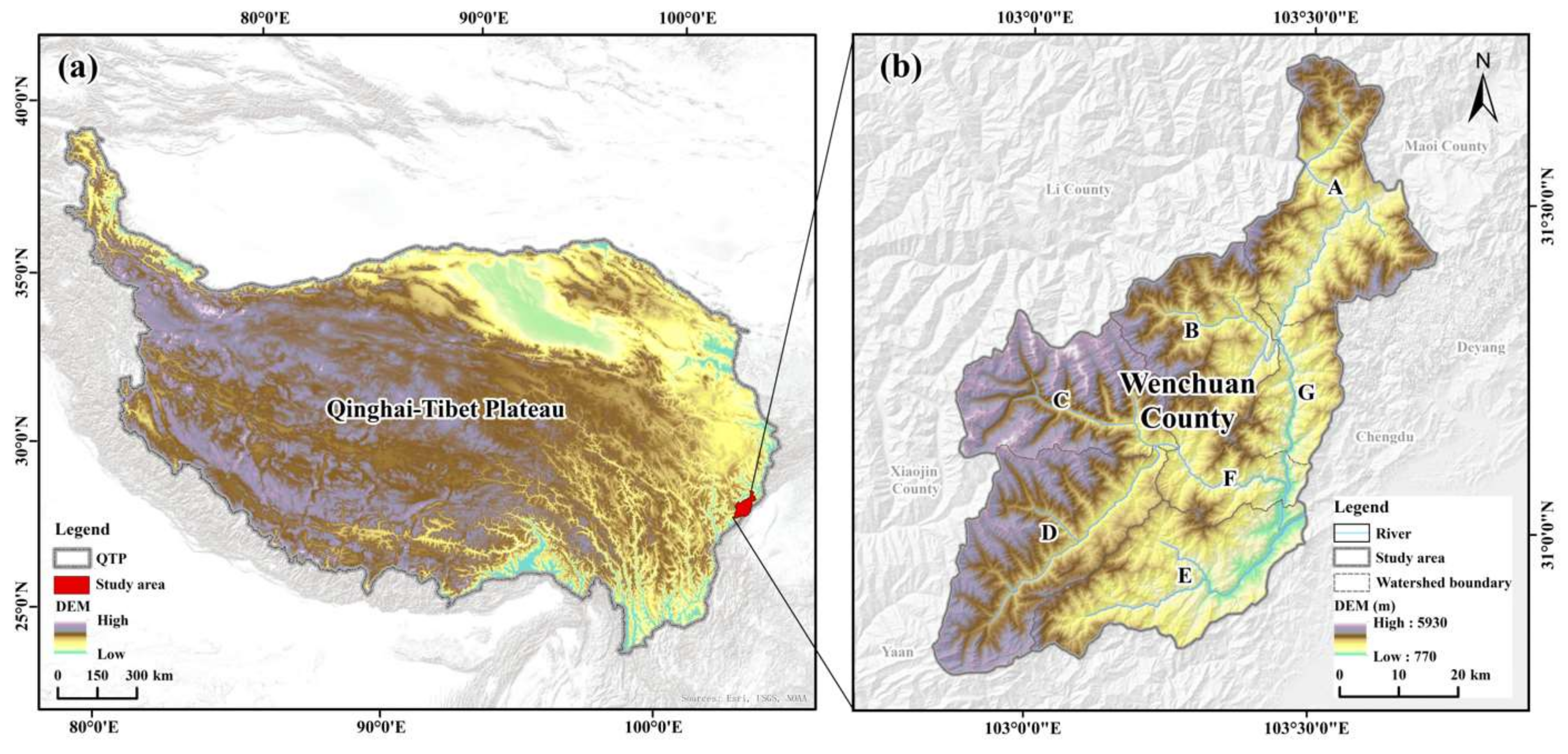
2.1. Study Area Overview
2.2. Data and Preprocessing
2.3. Methods
2.3.1. Ecological Indicators Assessment
2.3.2. Trade-Off/Synergy Analysis of Ecological Indicators
Correlation Analysis
Geographically Weighted Regression (GWR)
2.3.3. Identification of Ecological Indicator Bundles
2.3.4. Driving Force Analysis
3. Results
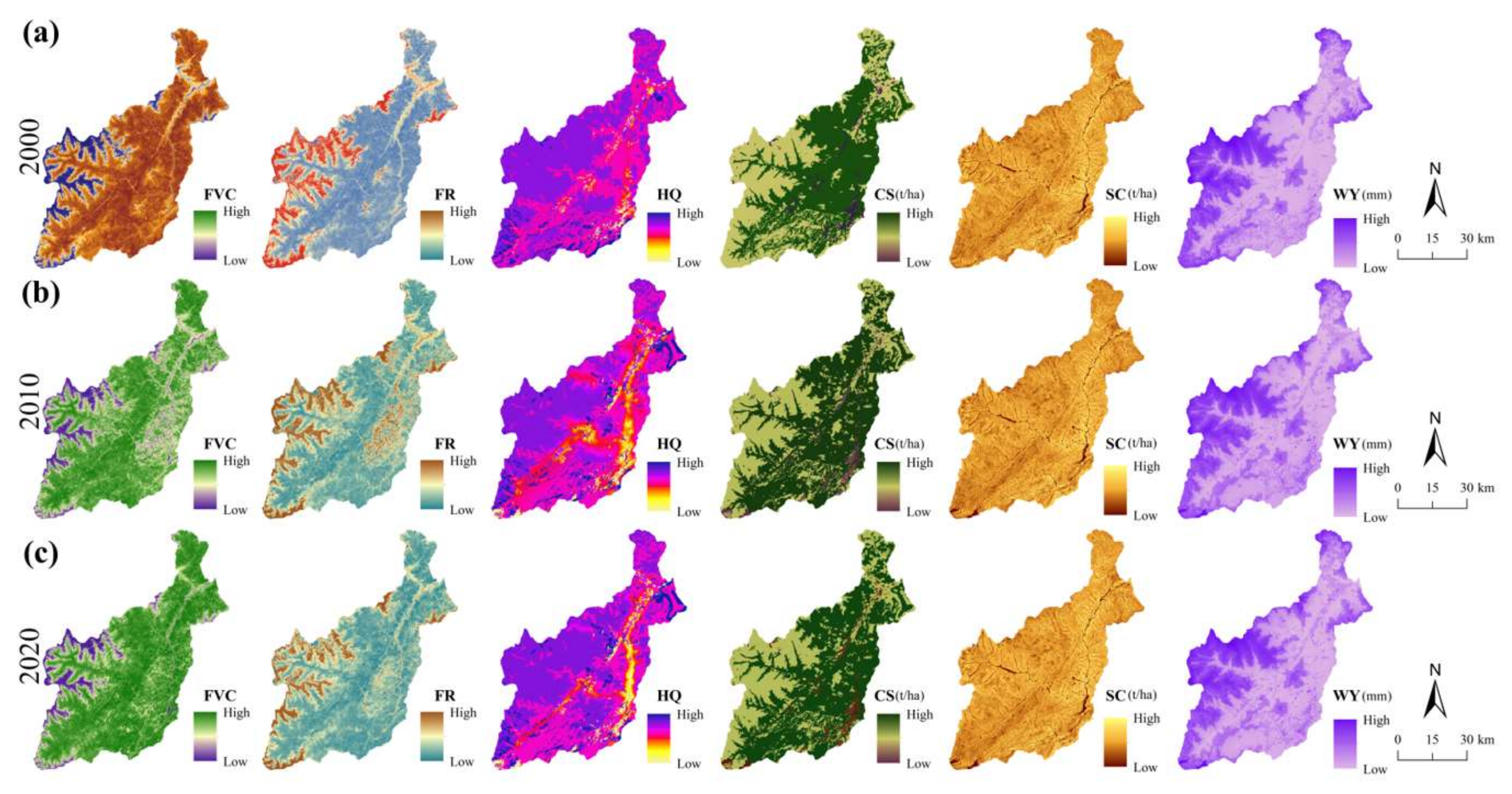
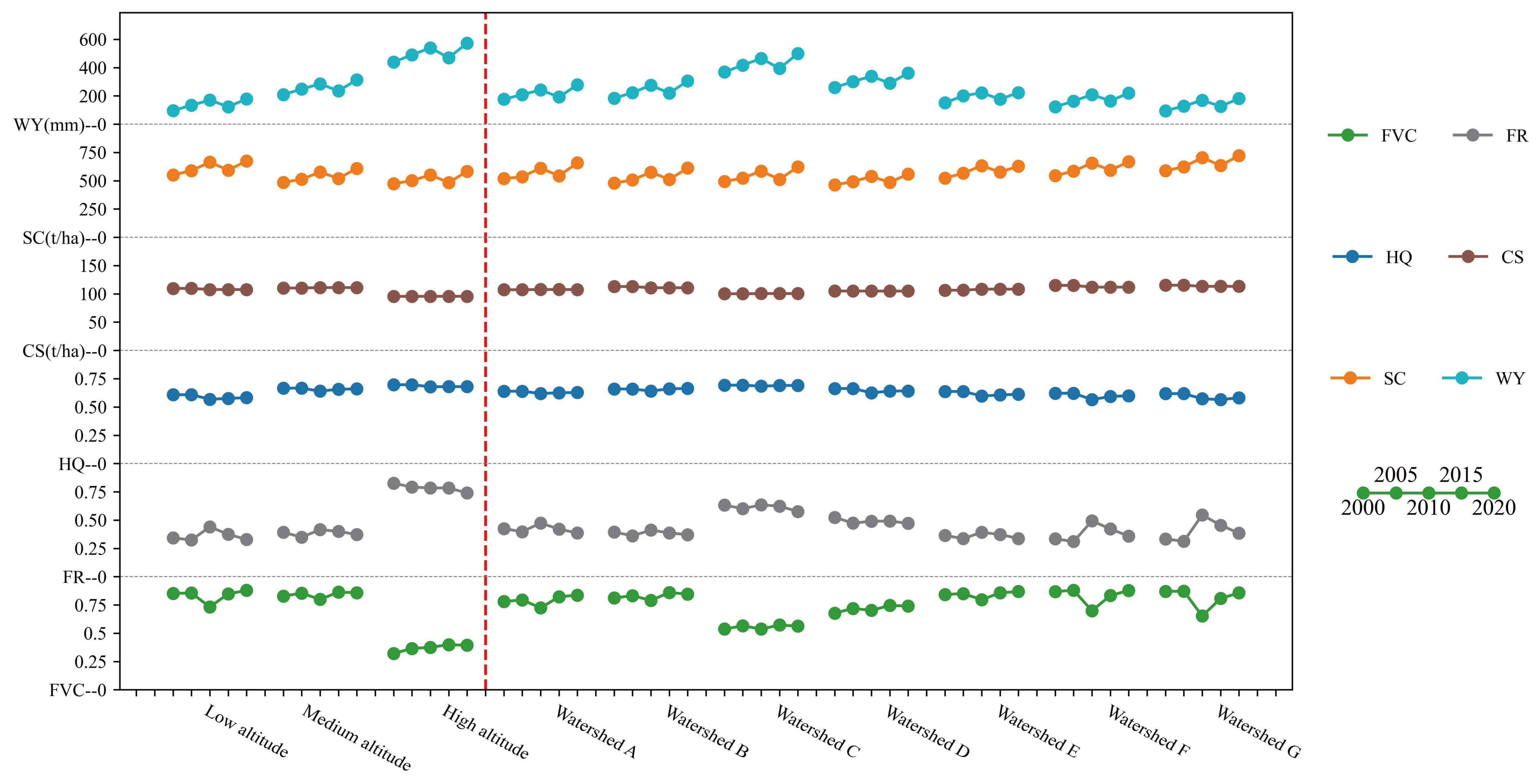
3.1. Spatiotemporal Distribution Characteristics
3.1.1. Spatial Distribution Characteristics
3.1.2. Temporal Variation Characteristics
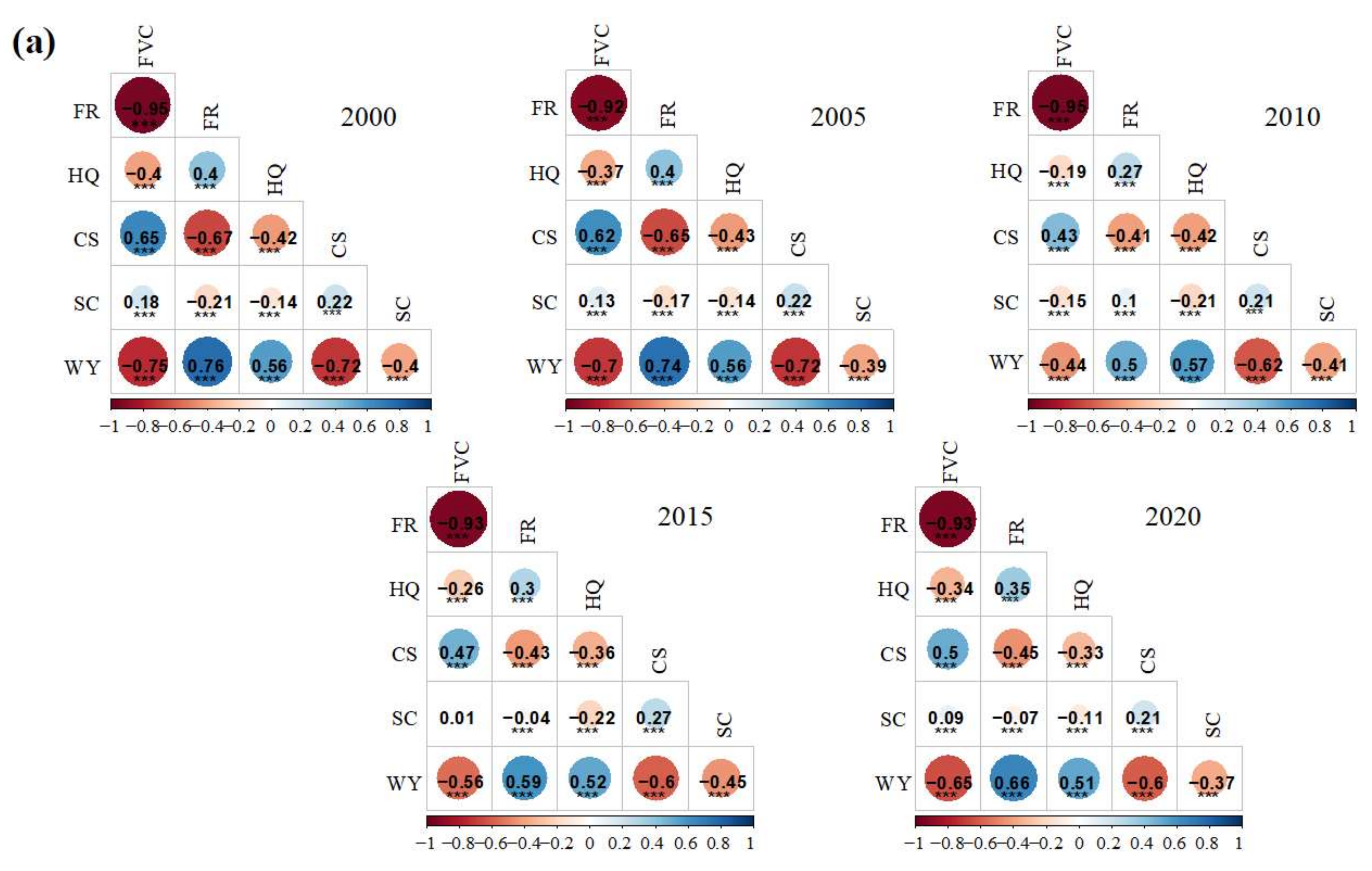
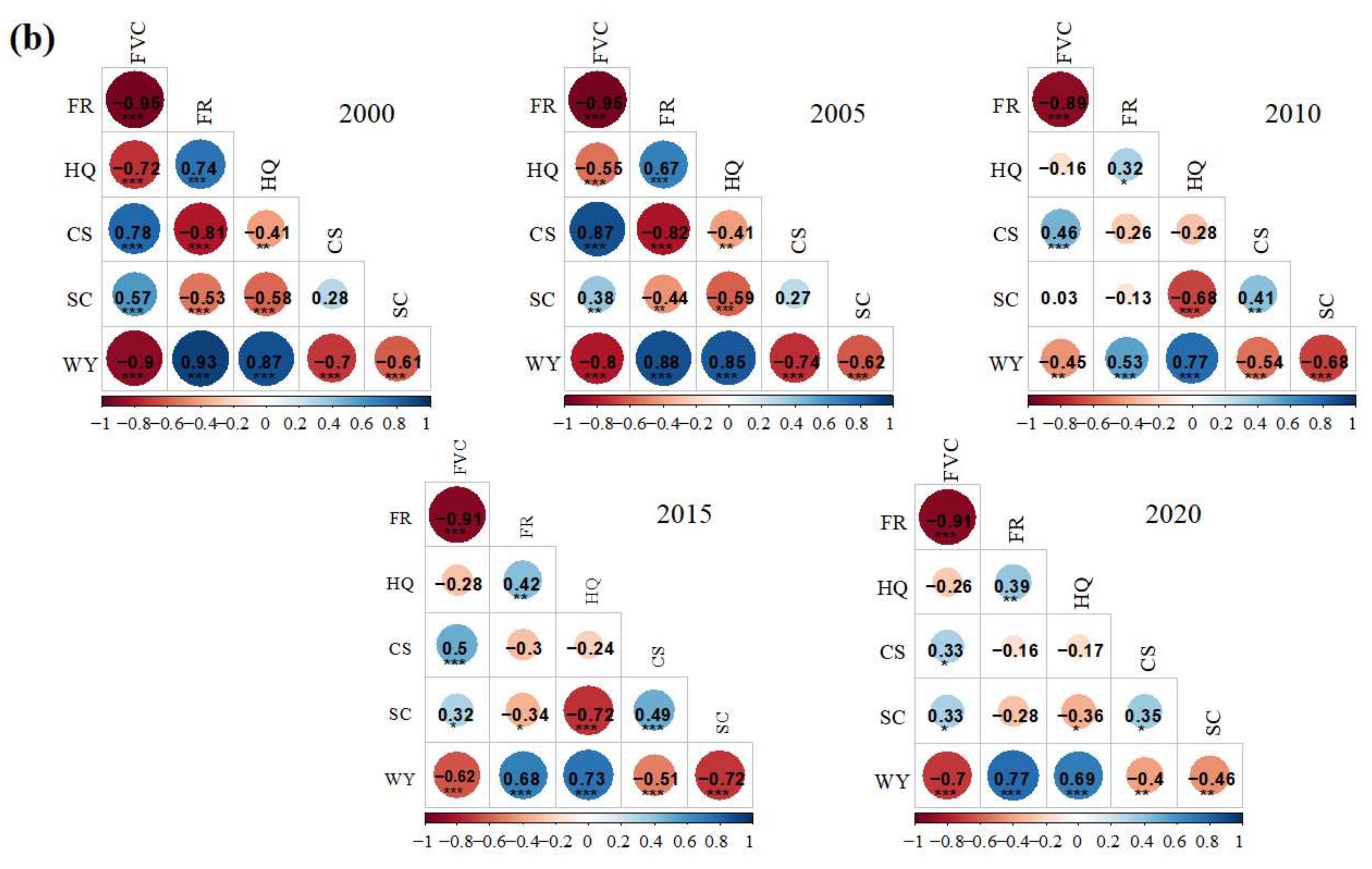
3.2. Trade-Offs and Synergies Between Ecological Indicators
3.2.1. Results of Correlation Analysis
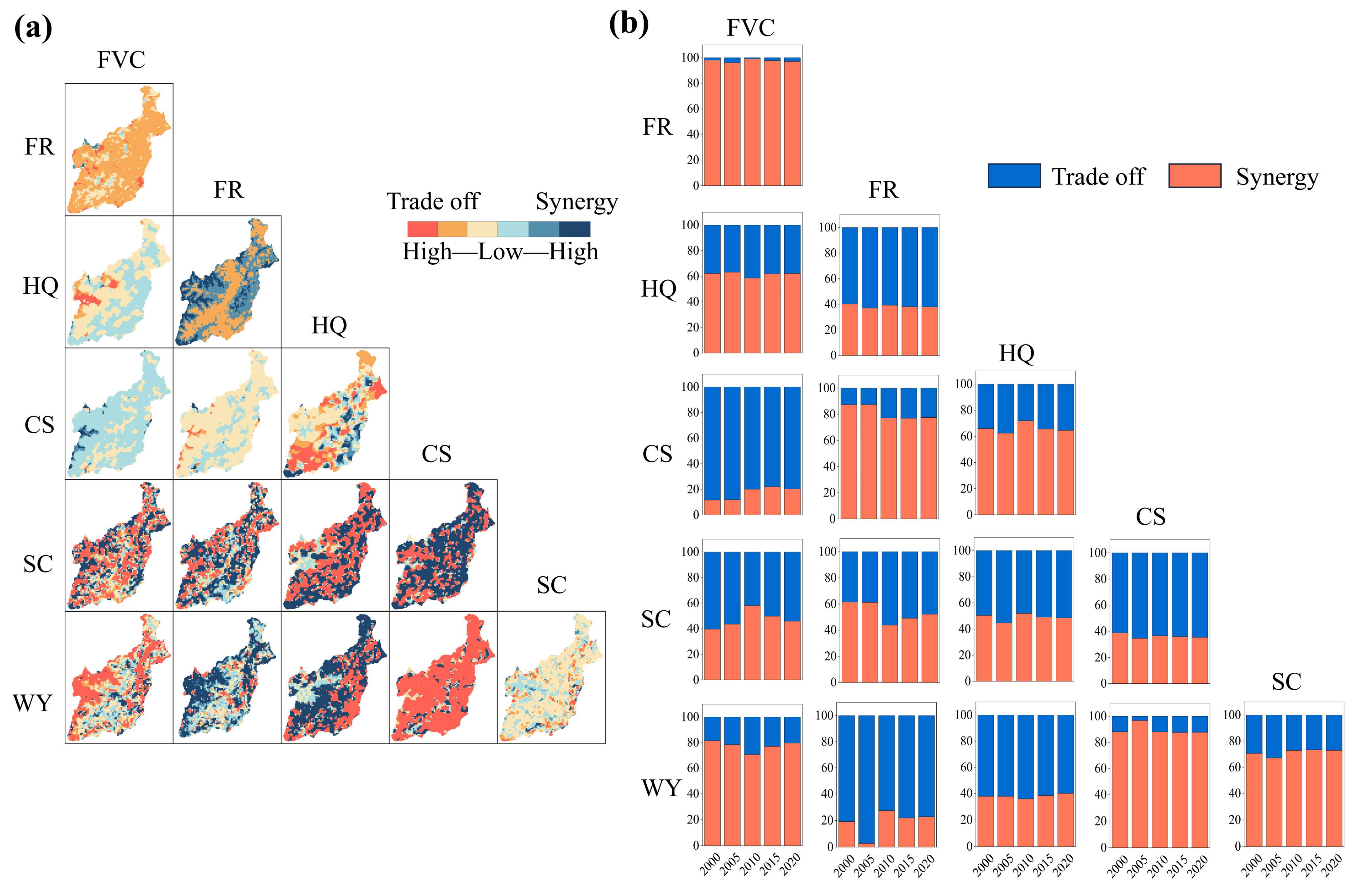
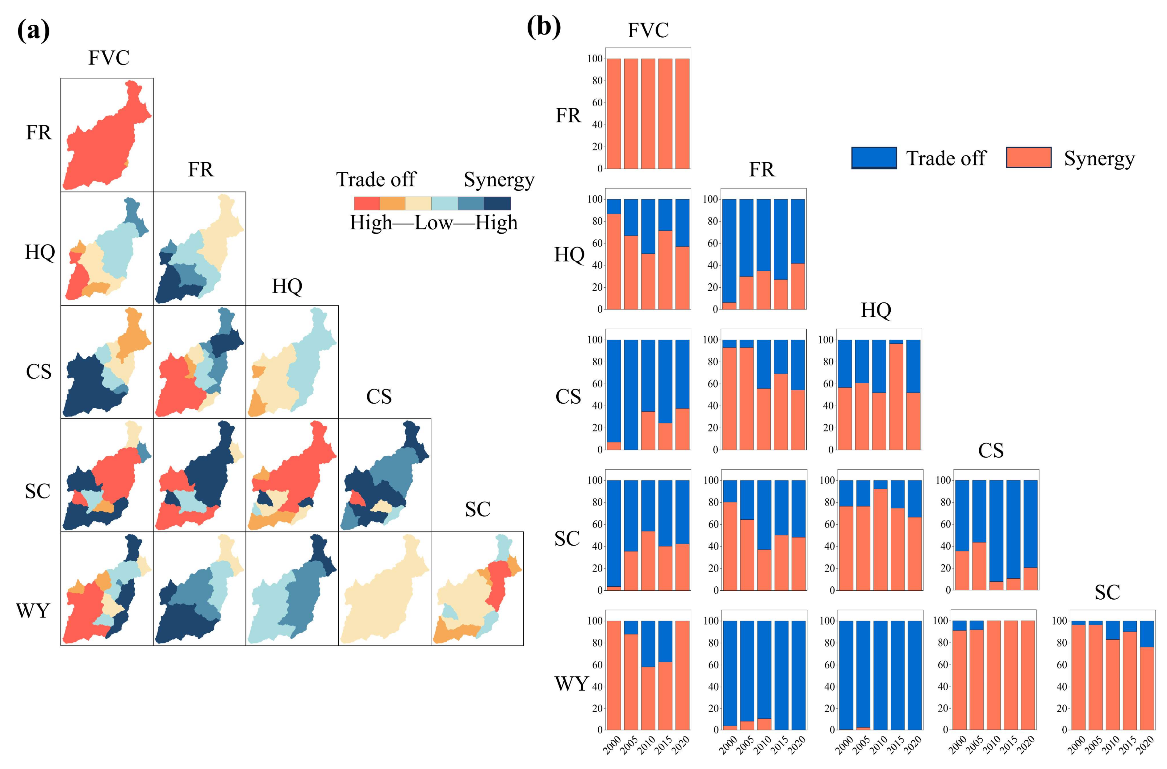
3.2.2. Results of GWR
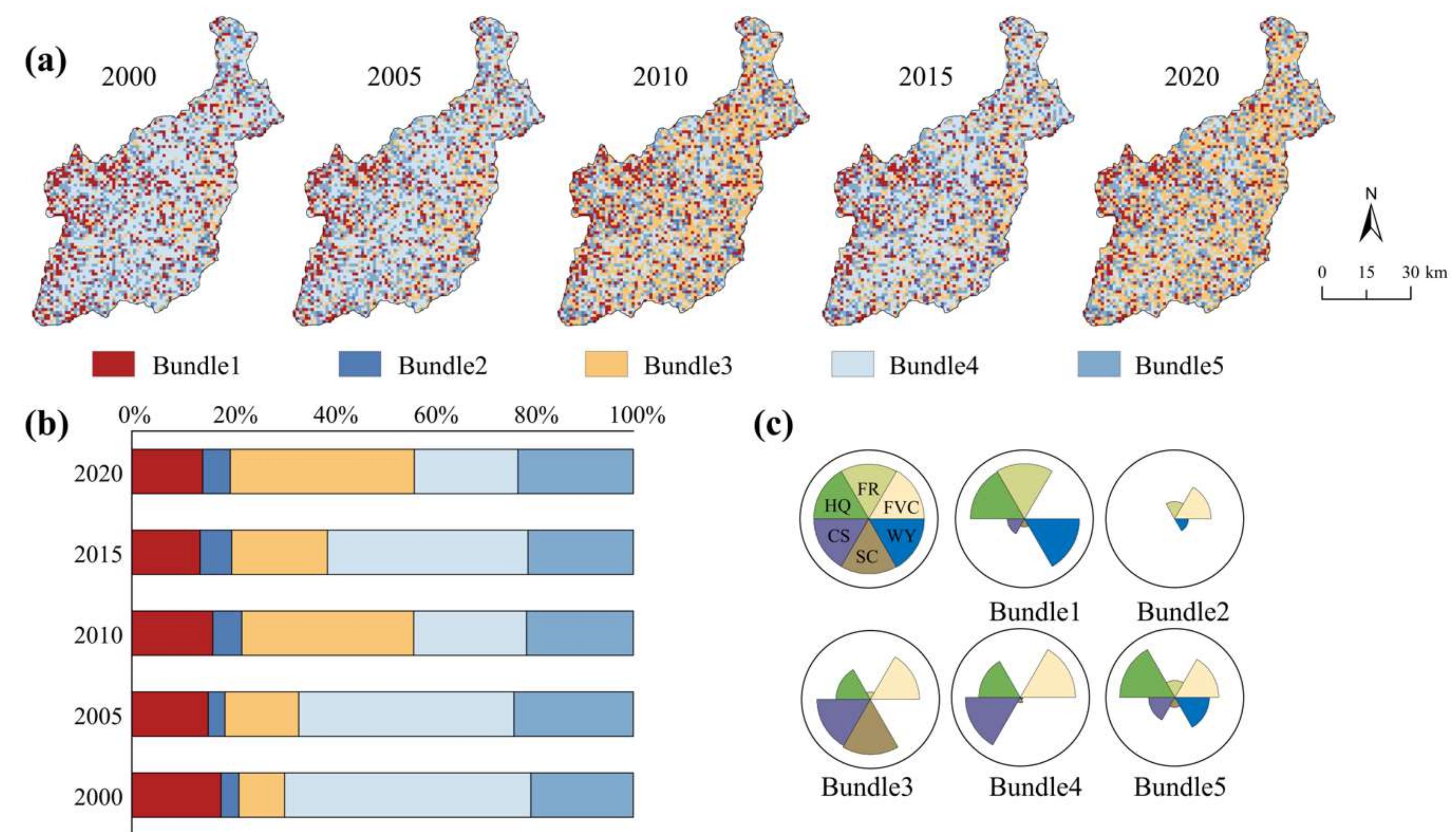
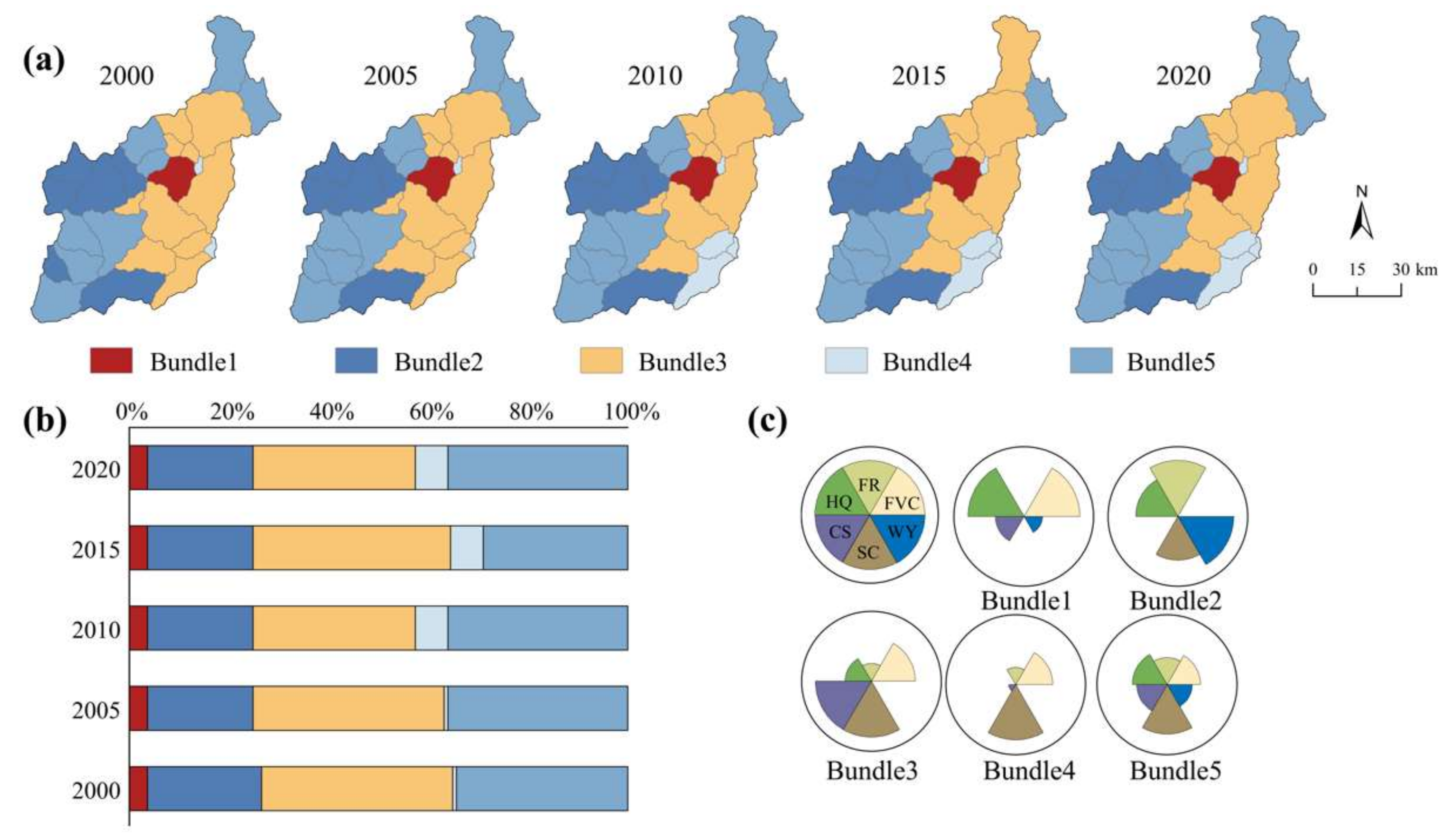
3.3. Identification of Ecological Indicator Bundles
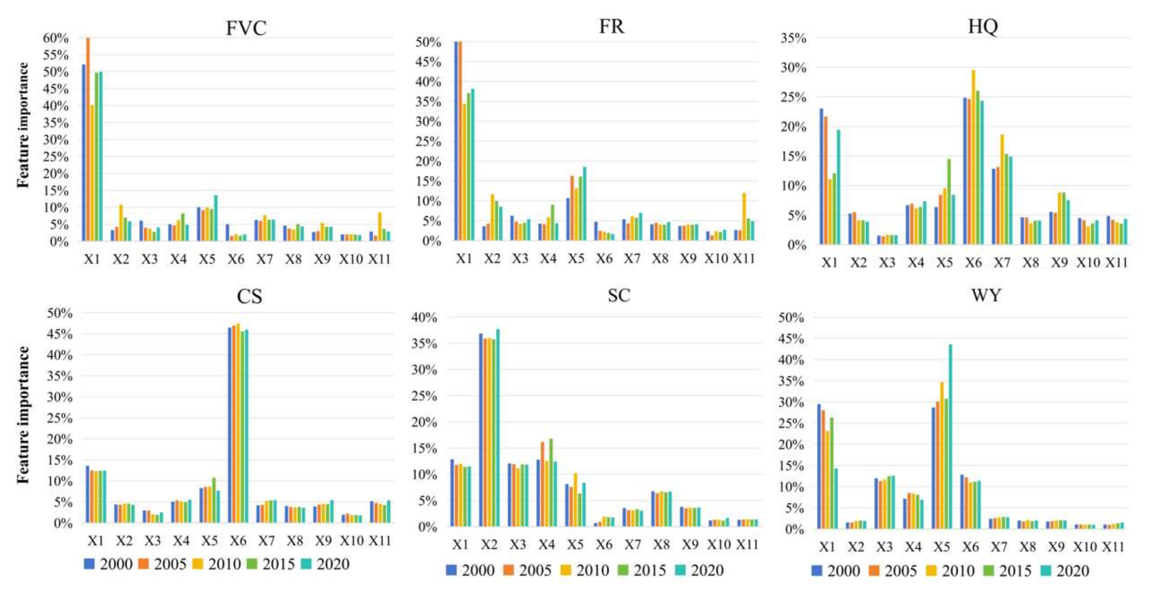
3.4. Results of Driving Force Analysis
4. Discussion
4.1. Spatiotemporal Evolution of LC and ESs
4.2. Interactions Between LC and ESs
4.3. Analysis of Driving Mechanisms
4.4. Significance of the Study and Policy Recommendations
4.5. Limitations and Prospects
5. Conclusions
- (1)
- The spatial distribution of ecological indicators exhibited a significant “gradient effect”: FVC, CS, and SC decreased with increasing elevation, showing a “high in the east, low in the west” distribution pattern; FR, HQ, and WY increased with increasing elevation, showing a “high in the west, low in the east” distribution pattern.
- (2)
- The earthquake had a significant but periodic impact on LC. Post-earthquake, FVC showed a “V”-shaped fluctuation, while FR showed an inverted “V”-shaped fluctuation. However, in most areas, vegetation and rock exposure had recovered to pre-earthquake levels by 2015, indicating a clear “recovery period”. In contrast, ESs were less affected by the earthquake. HQ and CS decreased slightly after the earthquake, while SC and WY showed an upward trend driven by climate change from 2000 to 2020.
- (3)
- Ecological indicators could be divided into two groups based on trade-off and synergy relationships. One group consists of FVC, CS, and SC, while the other group consists of FR, HQ, and WY. Ecological indicators within the same group exhibited synergy, while those between different groups exhibited trade-offs. The trade-off and synergy relationships of ecological indicators were similar across different scales but were more pronounced at larger scales and showed strong spatial heterogeneity.
- (4)
- Ecological indicators were driven by both natural and human factors, with elevation being a key driving factor. Elevation (explainability > 45%) was the primary driver of FVC and FR, and the earthquake temporarily enhanced the driving effect of lithology. The spatial distribution and variation of ESs are driven by multiple factors, including topography, climate, and human activities, all of which are closely related to the elevation gradient.
Author Contributions
Funding
Institutional Review Board Statement
Informed Consent Statement
Data Availability Statement
Conflicts of Interest
Appendix A

| Type | Formula | |
|---|---|---|
| Coverage Indicators | NDVI | |
| Where and are the red band and the near-infrared band of remote sensing images (Landsat TM/OLI), respectively. | ||
| NDRI | ||
| where and are the short-wave infrared band-1 and the near-infrared band of remote sensing images (Landsat TM/OLI), respectively. | ||
| Ecosystem Service | Habitat quality | |
| Here, Qxj represents the habitat quality of a grid within habitat type j, where Dxj indicates the disturbance level experienced by grid in habitat type . The constant is the half-saturation value, typically set at half of the maximum value obtained from during a preliminary trial, and , denotes the suitability of habitat type . | ||
| Carbon storage | ||
| In this equation, denotes above-ground organic matter, denotes below-ground organic matter, represents dead organic matter, and represents soil organic matter. | ||
| Ecosystem Service | Soil conservation | |
| In this equation, represents soil conservation capacity, while , denote potential and actual soil erosion, respectively. , , , , and represent rainfall erosivity, soil erodibility, slope length, vegetation cover management, and soil conservation practices. | ||
| Water yield | ||
| In this equation, represents the water yield for pixel ; : the annual precipitation for pixel ; and represents the annual evapotranspiration for pixel . | ||
| Spearman’s correlation analysis | ||
| where is the correlation coefficient between and ; and are the sample values of and , respectively; and is the number of samples. | ||
| Geographically Weighted Regression (GWR) | ||
| where is the sample values at position , is the remained sample values at position ; are the spatial coordinates of sampling point ; is the intercept term; is the regression coefficient and is the error term. | ||
| Extreme Gradient Boosting model (XGBoost model) | ||
| where represents the loss function, indicates the regularization term that suppresses the overfitting of the base learner at each iteration, and it is not involved in the integration of the final model. corresponds to the first-order derivative of the loss function, refers to the second-order derderivative of the loss function, and denotes the iteration number. | ||
| Shapley Additive Explanations (SHAP) | ||
| where is the SHAP value for a specific feature , indicating its influence on the model’s prediction. This value is computed by evaluating the contributions of feature across all potential subsets of the other features (excluding ). | ||
Appendix B. XGBoost-SHAP Model Evaluation Metrics
| 2000 | 2005 | 2010 | 2015 | 2020 | |||||||||||
|---|---|---|---|---|---|---|---|---|---|---|---|---|---|---|---|
| R2 | MAE | RMSE | R2 | MAE | RMSE | R2 | MAE | RMSE | R2 | MAE | RMSE | R2 | MAE | RMSE | |
| FVC | 0.96 | 0.04 | 0.05 | 0.96 | 0.03 | 0.05 | 0.92 | 0.05 | 0.06 | 0.94 | 0.04 | 0.06 | 0.94 | 0.04 | 0.06 |
| FR | 0.94 | 0.05 | 0.07 | 0.94 | 0.04 | 0.06 | 0.89 | 0.05 | 0.08 | 0.91 | 0.05 | 0.07 | 0.91 | 0.05 | 0.07 |
| HQ | 0.69 | 0.04 | 0.05 | 0.69 | 0.04 | 0.05 | 0.78 | 0.04 | 0.05 | 0.78 | 0.04 | 0.05 | 0.78 | 0.03 | 0.05 |
| CS | 0.82 | 0.03 | 0.05 | 0.82 | 0.03 | 0.05 | 0.81 | 0.04 | 0.06 | 0.80 | 0.04 | 0.06 | 0.81 | 0.04 | 0.06 |
| SC | 0.89 | 0.03 | 0.04 | 0.89 | 0.03 | 0.04 | 0.88 | 0.03 | 0.04 | 0.90 | 0.02 | 0.03 | 0.89 | 0.03 | 0.04 |
| WY | 0.96 | 0.04 | 0.05 | 0.96 | 0.04 | 0.05 | 0.95 | 0.04 | 0.05 | 0.95 | 0.04 | 0.05 | 0.96 | 0.04 | 0.05 |
| 2000 | 2005 | 2010 | 2015 | 2020 | |||||||||||
|---|---|---|---|---|---|---|---|---|---|---|---|---|---|---|---|
| R2 | MAE | RMSE | R2 | MAE | RMSE | R2 | MAE | RMSE | R2 | MAE | RMSE | R2 | MAE | RMSE | |
| FVC | 0.8 | 0.14 | 0.16 | 0.7 | 0.14 | 0.18 | × | 0.16 | 0.21 | 0.69 | 0.14 | 0.18 | 0.76 | 0.13 | 0.17 |
| FR | 0.77 | 0.18 | 0.19 | 0.7 | 0.15 | 0.19 | 0.52 | 0.18 | 0.21 | 0.65 | 0.14 | 0.18 | 0.61 | 0.17 | 0.20 |
| HQ | × | 0.13 | 0.19 | × | 0.15 | 0.21 | × | 0.14 | 0.19 | × | 0.15 | 0.19 | × | 0.14 | 0.18 |
| CS | × | 0.25 | 0.28 | × | 0.26 | 0.3 | × | 0.28 | 0.34 | × | 0.28 | 0.35 | × | 0.26 | 0.33 |
| SC | × | 0.15 | 0.27 | × | 0.15 | 0.26 | × | 0.15 | 0.27 | × | 0.16 | 0.28 | × | 0.15 | 0.28 |
| WY | 0.85 | 0.11 | 0.14 | 0.82 | 0.12 | 0.15 | 0.83 | 0.13 | 0.14 | 0.81 | 0.13 | 0.15 | 0.84 | 0.12 | 0.13 |
| Full Form | Abbreviation | Full Form | Abbreviation |
|---|---|---|---|
| Land cover | LC | Ecosystem service | ES |
| Fractional vegetation coverage | FVC | Rock exposure rate | FR |
| Habitat quality | HQ | Carbon storage | CS |
| Soil conservation | SC | Water yield | WY |
| Normalized difference vegetation index | NDVI | Normalized difference rock index | NDRI |
| Geographically weighted regression | GWR | Self-organizing map | SOM |
| Extreme gradient boosting | XGBoost | Shapley additive explanations | SHAP |
References
- Fan, X.; Juang, C.H.; Wasowski, J.; Huang, R.; Xu, Q.; Scaringi, G.; van Westen, C.J.; Havenith, H. What we have learned from the 2008 Wenchuan Earthquake and its aftermath: A decade of research and challenges. Eng. Geol. 2018, 241, 25–32. [Google Scholar] [CrossRef]
- Huang, R.; Li, W. Post-earthquake landsliding and long-term impacts in the Wenchuan earthquake area, China. Eng. Geol. 2014, 182, 111–120. [Google Scholar] [CrossRef]
- Cui, P.; Lin, Y.; Chen, C. Destruction of vegetation due to geo-hazards and its environmental impacts in the Wenchuan earthquake areas. Ecol. Eng. 2012, 44, 61–69. [Google Scholar] [CrossRef]
- Di, B.; Zeng, H.; Zhang, M.; Ustin, S.L.; Tang, Y.; Wang, Z.; Chen, N.; Zhang, B. Quantifying the spatial distribution of soil mass wasting processes after the 2008 earthquake in Wenchuan, China. Remote Sens. Environ. 2010, 114, 761–771. [Google Scholar] [CrossRef]
- Zhang, Y.; Zhao, X.; Gong, J.; Luo, F.; Pan, Y. Effectiveness and driving mechanism of ecological restoration efforts in China from 2009 to 2019. Sci. Total Environ. 2024, 910, 168676. [Google Scholar] [CrossRef]
- Duan, Y.; Di, B.; Ustin, S.L.; Xu, C.; Xie, Q.; Wu, S.; Li, J.; Zhang, R. Changes in ecosystem services in a montane landscape impacted by major earthquakes: A case study in Wenchuan earthquake-affected area, China. Ecol. Indic. 2021, 126, 107683. [Google Scholar] [CrossRef]
- Zhang, J.; Zhang, Y.; Dannenberg, M.P.; Guo, Q.; Atkins, J.W.; Li, W.; Sun, G. Eco-hydrological recovery following large vegetation disturbances from a mega earthquake on the eastern Tibetan plateau. J. Hydrol. 2025, 651, 132595. [Google Scholar] [CrossRef]
- Qiu, H.; Zhang, J.; Han, H.; Cheng, X.; Kang, F. Study on the impact of vegetation change on ecosystem services in the Loess Plateau, China. Ecol. Indic. 2023, 154, 110812. [Google Scholar] [CrossRef]
- Zhao, Z.; Dai, E. Vegetation cover dynamics and its constraint effect on ecosystem services on the Qinghai-Tibet Plateau under ecological restoration projects. J. Environ. Manag. 2024, 356, 120535. [Google Scholar] [CrossRef]
- Li, C.; Qiao, W.; Gao, B.; Chen, Y. Unveiling spatial heterogeneity of ecosystem services and their drivers in varied landform types: Insights from the Sichuan-Yunnan ecological barrier area. J. Clean. Prod. 2024, 442, 141158. [Google Scholar] [CrossRef]
- Pei, R.; Ma, B.; Liu, S.; Su, J.; Yu, M.; Li, W. Spatiotemporal differentiation and trade-offs and synergies of ecosystem services in Qilian Mountains National Park. Ecol. Indic. 2024, 169, 112891. [Google Scholar]
- Wang, Q.; Yao, Y.; Zhao, L.; Yang, C.; Zhao, Y.; Zhang, Q. Enhancing resilience against geological hazards and soil erosion through sustainable vegetation management: A case study in Shaanxi Province. J. Clean. Prod. 2023, 423, 138687. [Google Scholar]
- Wang, W.; Pen, Y.; Xu, W.; Wang, J.; Bai, X. Analysis on Ecosystem Destroy and lts Ecological impact Caused by Earthquake in Wenchuan, Sichuan Province. Res. Environ. Sci. 2008, 21, 110–116. [Google Scholar]
- Zhou, Q.; Chen, W.; Wang, H.; Wang, D. Spatiotemporal evolution and driving factors analysis of fractional vegetation coverage in the arid region of northwest China. Sci. Total Environ. 2024, 954, 176271. [Google Scholar] [PubMed]
- Wang, X.; Fan, X.; Fang, C.; Dai, L.; Zhang, W.; Zheng, H.; Xu, Q. Long-Term Landslide Evolution and Restoration After the Wenchuan Earthquake Revealed by Time-Series Remote Sensing Images. Geophys. Res. Lett. 2024, 51, e2023GL106422. [Google Scholar]
- Pu, J.; Zhao, X.; Huang, P.; Gu, Z.; Shi, X.; Chen, Y.; Shi, X.; Tao, J.; Xu, Y.; Xiang, A. Ecological risk changes and their relationship with exposed surface fraction in the karst region of southern China from 1990 to 2020. J. Environ. Manag. 2022, 323, 116206. [Google Scholar]
- Yang, W.; Qi, W.; Zhou, J. Decreased post-seismic landslides linked to vegetation recovery after the 2008 Wenchuan earthquake. Ecol. Indic. 2018, 89, 438–444. [Google Scholar]
- Shen, P.; Zhang, L.M.; Fan, R.L.; Zhu, H.; Zhang, S. Declining geohazard activity with vegetation recovery during first ten years after the 2008 Wenchuan earthquake. Geomorphology 2020, 352, 106989. [Google Scholar]
- Liu, Q.; Li, Y. Examining the Spatiotemporal Evolution of Land Use Conflicts from an Ecological Security Perspective: A Case Study of Tianshui City, China. Sustainability 2025, 17, 2253. [Google Scholar] [CrossRef]
- Zeng, W.; He, L.; He, Z.; Zhao, Y.; Yuan, Y.; Pang, J.; Zhao, J. A Prediction–Interaction–Driving Framework for Ecosystem Services Under Climate Change and Human Activities: A Case Study of Zoigê Plateau. Land 2025, 14, 441. [Google Scholar] [CrossRef]
- Chen, Y.; Zhang, F.; Lin, J. Projecting Future Land Use Evolution and Its Effect on Spatiotemporal Patterns of Habitat Quality in China. Appl. Sci. 2025, 15, 1042. [Google Scholar] [CrossRef]
- Wang, B.; Li, X.; Ma, C.F.; Zhu, G.F.; Luan, W.F.; Zhong, J.T.; Tan, M.B.; Fu, J. Uncertainty analysis of ecosystem services and implications for environmental management—An experiment in the Heihe River Basin, China. Sci. Total Environ. 2022, 821, 153481. [Google Scholar]
- Hamel, P.; Bryant, B.P. Uncertainty assessment in ecosystem services analyses: Seven challenges and practical responses. Ecosyst. Serv. 2017, 24, 1–15. [Google Scholar]
- Pan, Z.; Gao, G.; Fu, B. Spatiotemporal changes and driving forces of ecosystem vulnerability in the Yangtze River Basin, China: Quantification using habitat-structure-function framework. Sci. Total Environ. 2022, 835, 155494. [Google Scholar] [PubMed]
- Liu, C.; Li, W.; Xu, J.; Zhou, H.; Wang, W.; Wang, H. Temporal and spatial variations of ecological security on the northeastern Tibetan Plateau integrating ecosystem health-risk-services framework. Ecol. Indic. 2024, 158, 111365. [Google Scholar]
- Su, N.; Xu, L.; Yang, B.; Li, Y.; Gu, F. Risk Assessment of Single-Gully Debris Flow Based on Dynamic Changes in Provenance in the Wenchuan Earthquake Zone: A Case Study of the Qipan Gully. Sustainability 2023, 15, 12098. [Google Scholar] [CrossRef]
- Xiao, L.; Zhou, J.; Wu, X.; Anas Khan, M.; Zhao, S.; Wu, X. The dominant influence of terrain and geology on vegetation mortality in response to drought: Exploring resilience and resistance. Catena 2024, 243, 108156. [Google Scholar]
- Li, Q.; Bao, Y.; Wang, Z.; Chen, X.; Lin, X. Trade-offs and synergies of ecosystem services in karst multi-mountainous cities. Ecol. Indic. 2024, 159, 111637. [Google Scholar]
- Xia, H.; Yuan, S.; Prishchepov, A.V. Spatial-temporal heterogeneity of ecosystem service interactions and their social-ecological drivers: Implications for spatial planning and management. Resour. Conserv. Recycl. 2023, 189, 106767. [Google Scholar]
- Gao, Y.; Wang, Z.; Li, C. Assessing spatio-temporal heterogeneity and drivers of ecosystem services to support zonal management in mountainous cities. Sci. Total Environ. 2024, 954, 176328. [Google Scholar]
- Xiao, H.; Shao, H.; Long, J.; Zhang, S.; He, S.; Wang, D. Spatial-temporal pattern evolution and geological influence factors analysis of ecological vulnerability in Western Sichuan mountain region. Ecol. Indic. 2023, 155, 110980. [Google Scholar]
- Zhang, L.; Li, X.; Liu, X.; Lian, Z.; Zhang, G.; Liu, Z.; An, S.; Ren, Y.; Li, Y.; Liu, S. Dynamic monitoring and drivers of ecological environmental quality in the Three-North region, China: Insights based on remote sensing ecological index. Ecol. Inform. 2025, 85, 102936. [Google Scholar]
- Wu, F.; Yang, X.; Cui, Z.; Ren, L.; Jiang, S.; Liu, Y.; Yuan, S. The impact of human activities on blue-green water resources and quantification of water resource scarcity in the Yangtze River Basin. Sci. Total Environ. 2024, 909, 168550. [Google Scholar] [CrossRef] [PubMed]
- Shaikh, S.F.E.A.; See, S.C.; Richards, D.; Belcher, R.N.; Grêt-Regamey, A.; Galleguillos Torres, M.; Carrasco, L.R. Accounting for spatial autocorrelation is needed to avoid misidentifying trade-offs and bundles among ecosystem services. Ecol. Indic. 2021, 129, 107992. [Google Scholar]
- Xiong, J.; Chen, H.; Tang, C.; Chen, M.; Chang, M.; Zhang, X.; Gong, L.; Li, N.; Shi, Q.; Li, M. Application of remote sensing monitoring to the spatiotemporal variation in debris flow activity in the catastrophic Wenchuan seismic area. Catena 2023, 232, 107450. [Google Scholar] [CrossRef]
- Mukhopadhyay, A.; Hati, J.P.; Acharyya, R.; Pal, I.; Tuladhar, N.; Habel, M. Global trends in using the InVEST model suite and related research: A systematic review. Ecohydrol. Hydrobiol. 2024; in press. [Google Scholar] [CrossRef]
- Yang, R.; Mu, Z.; Gao, R.; Huang, M.; Zhao, S. Interactions between ecosystem services and their causal relationships with driving factors: A case study of the Tarim River Basin, China. Ecol. Indic. 2024, 169, 112810. [Google Scholar] [CrossRef]
- Zhao, T.; Pan, J. Ecosystem service trade-offs and spatial non-stationary responses to influencing factors in the Loess hilly-gully region: Lanzhou City, China. Sci. Total Environ. 2022, 846, 157422. [Google Scholar]
- Chang, B.; Chen, B.; Chen, W.; Xu, S.; He, X.; Yao, J.; Huang, Y. Analysis of trade-off and synergy of ecosystem services and driving forces in urban agglomerations in Northern China. Ecol. Indic. 2024, 165, 112210. [Google Scholar] [CrossRef]
- Li, W.; Kang, J.; Wang, Y. Exploring the interactions and driving factors among typical ecological risks based on ecosystem services: A case study in the Sichuan-Yunnan ecological barrier area. Ecol. Indic. 2025, 170, 113000. [Google Scholar] [CrossRef]
- Qu, J.; Xu, Z.; Dong, B.; Wang, H.; Han, Y. Analyzing trade-offs, synergies, and driving factors of ecosystem services in Anhui Province using spatial analysis and XG-boost modeling. Ecol. Indic. 2025, 171, 113098. [Google Scholar]
- Dai, F.C.; Xu, C.; Yao, X.; Xu, L.; Tu, X.B.; Gong, Q.M. Spatial distribution of landslides triggered by the 2008 Ms 8.0 Wenchuan earthquake, China. J. Asian Earth Sci. 2011, 40, 883–895. [Google Scholar]
- Huang, R.; Li, W. Development and distribution of geohazards triggered by the 5.12 Wenchuan Earthquake in China. Sci. China Ser. E Technol. Sci. 2009, 52, 810–819. [Google Scholar]
- Lv, J.; He, X.; Bao, Y.; Li, H. Spatiotemporal pattern of post-earthquake vegetation recovery in a mountainous catchment in southwestern China. Nat. Hazards 2024, 121, 3023–3046. [Google Scholar]
- Fusun, S.; Jinniu, W.; Tao, L.; Yan, W.; Haixia, G.; Ning, W. Effects of different types of vegetation recovery on runoff and soil erosion on a Wenchuan earthquake-triggered landslide, China. J. Soil Water Conserv. 2013, 68, 138–145. [Google Scholar]
- Zhang, S.; Zhang, L.M. Impact of the 2008 Wenchuan earthquake in China on subsequent long-term debris flow activities in the epicentral area. Geomorphology 2017, 276, 86–103. [Google Scholar]
- Tang, C.; Zhu, J.; Qi, X.; Ding, J. Landslides induced by the Wenchuan earthquake and the subsequent strong rainfall event: A case study in the Beichuan area of China. Eng. Geol. 2011, 122, 22–33. [Google Scholar]
- Niu, C.; Huang, C.; Zhang, X.; Ma, S.; Wang, L.; Hu, H.; Jiang, J. Trends in the Altitudinal Gradient Evolution of Vegetation Ecological Functions in Mountainous Areas. Forests 2024, 15, 1000. [Google Scholar] [CrossRef]
- Duan, L.; Yang, S.; Xiang, M.; Li, W.; Li, J. Spatiotemporal evolution and driving factors of ecosystem service value in the Upper Minjiang River of China. Sci. Rep. 2024, 14, 23398. [Google Scholar]
- Chen, L.; Wang, Q. Study on the Contradiction between Population and Cultivated Land and the Priority Protection of Cultivated Land in the Policy of Poverty Alleviation: A Case Study of the Upper Reaches of Min River, Sichuan Province, China. Sustainability 2021, 13, 3348. [Google Scholar] [CrossRef]
- Jiao, Q.; Zhang, B.; Liu, L.; Li, Z.; Yue, Y.; Hu, Y. Assessment of spatio-temporal variations in vegetation recovery after the Wenchuan earthquake using Landsat data. Nat. Hazards 2014, 70, 1309–1326. [Google Scholar]
- Wu, X.; Liu, H.; Huang, X.; Zhou, T. Human driving forces: Analysis of rocky desertification in karst region in Guanling County, Guizhou Province. Chin. Geogr. Sci. 2011, 21, 600–608. [Google Scholar]
- Zhang, H.; Tang, Q.; He, X.; Yang, Q. Land use function changes and trade-offs/synergies across topographic gradients in the Three Gorges Reservoir Area, China. J. Clean. Prod. 2024, 469, 143233. [Google Scholar]
- Gao, J.; Bian, H.; Zhu, C.; Tang, S. The response of key ecosystem services to land use and climate change in Chongqing: Time, space, and altitude. J. Geogr. Sci. 2022, 32, 317–332. [Google Scholar]
- Wei, D.; Tao, J.; Wang, Z.; Zhao, H.; Zhao, W.; Wang, X. Elevation-dependent pattern of net CO2 uptake across China. Nat. Commun. 2024, 15, 2489. [Google Scholar]
- Ma, S.; Qiao, Y.; Wang, L.; Zhang, J. Terrain gradient variations in ecosystem services of different vegetation types in mountainous regions: Vegetation resource conservation and sustainable development. Forest Ecol. Manag. 2021, 482, 118856. [Google Scholar]
- Huang, L.; Du, Y.; Tang, Y. Ecosystem service trade-offs and synergies and their drivers in severely affected areas of the Wenchuan earthquake, China. Land. Degrad. Dev. 2024, 35, 3881–3896. [Google Scholar]
- Zhang, L.; Yu, K.; Zhang, Y.; Wei, J.; Yang, W.; Wang, X. Research on the Value of County-Level Ecosystem Services in Highly Mountainous Canyon Areas Based on Land Use Change: Analysis of Spatiotemporal Evolution Characteristics and Spatial Stability. Land 2025, 14, 398. [Google Scholar] [CrossRef]
- Zhang, J.; Xu, W.; Kong, L.; Hull, V.; Xiao, Y.; Xiao, Y.; Ouyang, Z. Strengthening protected areas for giant panda habitat and ecosystem services. Biol. Conserv. 2018, 227, 1–8. [Google Scholar]
- Zheng, D.; Wang, Y.; Hao, S.; Xu, W.; Lv, L.; Yu, S. Spatial-temporal variation and tradeoffs/synergies analysis on multiple ecosystem services: A case study in the Three-River Headwaters region of China. Ecol. Indic. 2020, 116, 106494. [Google Scholar]
- Qin, J.; Yang, B.; Ding, Y.; Cui, J.; Zhang, Y. Assessment of runoff generation capacity and total runoff contribution for different landscapes in alpine and permafrost watershed. Catena 2025, 249, 108643. [Google Scholar]
- Xu, J.; Wang, S.; Xiao, Y.; Xie, G.; Wang, Y.; Zhang, C.; Li, P.; Lei, G. Mapping the spatiotemporal heterogeneity of ecosystem service relationships and bundles in Ningxia, China. J. Clean. Prod. 2021, 294, 126216. [Google Scholar]
- Shen, J.; Li, S.; Liang, Z.; Liu, L.; Li, D.; Wu, S. Exploring the heterogeneity and nonlinearity of trade-offs and synergies among ecosystem services bundles in the Beijing-Tianjin-Hebei urban agglomeration. Ecosyst. Serv. 2020, 43, 101103. [Google Scholar]
- Zhai, J.; Wang, L.; Liu, Y.; Wang, C.; Mao, X. Assessing the effects of China’s Three-North Shelter Forest Program over 40 years. Sci. Total Environ. 2023, 857, 159354. [Google Scholar]
- Yang, L.; Li, Y.; Yu, L.; Chen, M.; Yu, M.; Zhang, Y. Theory and case of land use transition promoting ecological restoration in karst mountain areas of Southwest China. Ecol. Indic. 2024, 158, 111393. [Google Scholar]


| Data type | Format | Resolution | Data Source |
|---|---|---|---|
| Administrative boundaries | Shpfile | / | National Platform for Common Geospatial Information Services (www.tianditu.gov.cn) |
| Major road data | Shpfile | / | Open Street Map (www.openstreetmap.org) |
| Land use data | Raster | 30 m | Resource and Environment Science and Data Center(www.resdc.cn) |
| DEM | Raster | 30 m | Geospatial Data Cloud Platform (www.gscloud.cn) |
| Precipitation | Raster | 1000 m | National Tibetan Plateau Science Data Center (https://data.tpdc.ac.cn) |
| Evapotranspiration | Raster | 1000 m | National Tibetan Plateau Science Data Center (https://data.tpdc.ac.cn) |
| Soli type | Raster | 250 m | Harmonized Worldwide Soil Data base: (HWSD) (http://www.fao.org) |
| Geological data | Shpfile | / | Geoscientific Data and Discovery Publishing System (http://dcc.ngac.org.cn) |
| FVC | FR | HQ | CS | SC | WY | |
|---|---|---|---|---|---|---|
| R2 | 0.95 | 0.92 | 0.75 | 0.81 | 0.89 | 0.96 |
| MAE | 0.04 | 0.05 | 0.04 | 0.04 | 0.03 | 0.04 |
| RMSE | 0.06 | 0.07 | 0.05 | 0.06 | 0.04 | 0.05 |
Disclaimer/Publisher’s Note: The statements, opinions and data contained in all publications are solely those of the individual author(s) and contributor(s) and not of MDPI and/or the editor(s). MDPI and/or the editor(s) disclaim responsibility for any injury to people or property resulting from any ideas, methods, instructions or products referred to in the content. |
© 2025 by the authors. Licensee MDPI, Basel, Switzerland. This article is an open access article distributed under the terms and conditions of the Creative Commons Attribution (CC BY) license (https://creativecommons.org/licenses/by/4.0/).
Share and Cite
Pang, J.; He, L.; He, Z.; Zeng, W.; Yuan, Y.; Bai, W.; Zhao, J. Interactions and Driving Force of Land Cover and Ecosystem Service Before and After the Earthquake in Wenchuan County. Sustainability 2025, 17, 3094. https://doi.org/10.3390/su17073094
Pang J, He L, He Z, Zeng W, Yuan Y, Bai W, Zhao J. Interactions and Driving Force of Land Cover and Ecosystem Service Before and After the Earthquake in Wenchuan County. Sustainability. 2025; 17(7):3094. https://doi.org/10.3390/su17073094
Chicago/Turabian StylePang, Jintai, Li He, Zhengwei He, Wanting Zeng, Yan Yuan, Wenqian Bai, and Jiahua Zhao. 2025. "Interactions and Driving Force of Land Cover and Ecosystem Service Before and After the Earthquake in Wenchuan County" Sustainability 17, no. 7: 3094. https://doi.org/10.3390/su17073094
APA StylePang, J., He, L., He, Z., Zeng, W., Yuan, Y., Bai, W., & Zhao, J. (2025). Interactions and Driving Force of Land Cover and Ecosystem Service Before and After the Earthquake in Wenchuan County. Sustainability, 17(7), 3094. https://doi.org/10.3390/su17073094