Abstract
As a key pillar of China’s economy, the manufacturing industry faces sustainable financial risk management challenges as it undergoes digital and green low-carbon transformation. However, existing financial risk prediction models often suffer from limited accuracy, insufficient robustness, and a suboptimal activation function design. In this study, we investigated advanced deep learning architectures to address these limitations, and we introduced a novel composite triple activation function (CTAF) framework to enhance predictive performance and model robustness. We began by evaluating several deep learning models, such as CNNs, BiLSTM, CNN-AM, and BiLSTM-AM, demonstrating that CNN-BiLSTM-AM achieved the highest performance. On the basis of this model structure, we proposed a CTAF, a composite activation mechanism that combines two distinct functions applied to the raw input x, effectively mitigating gradient instability and enhancing nonlinear expressiveness. Through ablation experiments with different composite activation functions, we verified that the CTAF consistently outperformed alternatives. Meanwhile, the mainstream activation functions and CTAF were applied to different layers for comparison, further verifying the CTAF’s advantages in various structures. The optimal configuration was achieved when tanh was used in the CNN and Dense layers and the CTAF (tanh_relu) was applied in a Lambda layer after a BiLSTM layer, resulting in the highest accuracy of 99.5%. Furthermore, paired t-tests and evaluations on cross-industry datasets confirmed the optimal model’s stability and generalizability.
1. Introduction
As the core pillar of the Chinese economy, manufacturing has always held an important position in the national economy. In 2024, while maintaining growth, China’s manufacturing industry faced deep-seated industrial adjustments and sustainable development challenges. The added value of industrial enterprises above the designated size increased by 5.8% year on year, while the high-tech manufacturing industry grew by 8.9%, demonstrating the driving force of technological innovation. However, with the advancement of the “dual carbon” target, the restructuring of the global industrial chain, and the acceleration of digital transformation, manufacturing enterprises face more significant pressure regarding green development, technological upgrading, and market competition. In this context, the development differentiation of different industries has become increasingly evident, and some industries have encountered severe challenges in adapting to changes, leading to increased financial risks.
In this transformation process, the semiconductor, automotive manufacturing, and steel industries, as important components of China’s manufacturing industry, have experienced significant market fluctuations in recent years. In the semiconductor industry, 14,648 enterprises have gone bankrupt, reflecting the dual impact of global supply chain adjustment and domestic industrial structure upgrading. The profit of the automobile manufacturing industry has decreased by 7.3% year on year, and 24 vehicle manufacturers withdrew from the market between 2020 and 2024, accelerating the transformation of the new energy industry and promoting the survival of the fittest. The capacity utilization rate of the steel industry has dropped below 70%, and 2314 steel companies have incurred losses. Under the dual pressure of low-carbon transformation and market supply and demand adjustment, the industry faces the challenges of capacity optimization and green upgrading. These changes indicate that China’s manufacturing industry is at a critical stage driven by technological change and sustainable development goals. Balancing industrial upgrading with financial stability and improving enterprise risk response capabilities has become an urgent issue that needs to be addressed.
With the development of artificial intelligence, deep learning has shown significant advantages in financial risk prediction, especially convolutional neural networks (CNNs), bidirectional extended short-term memory (BiLSTM) networks, and attention mechanisms (AMs). CNNs can extract local features, BiLSTM networks are suitable for processing time series information, and AMs enhance a model’s attention to key features. However, existing models still have shortcomings in selecting activation functions and structural design, making it challenging to fully explore the complex relationships in financial data.
Therefore, in this study, we propose a CNN-BiLSTM-AM model optimized based on a composite triple activation function (CTAF). The CTAF combines two activation functions with a multiplication scaling term to improve gradient propagation efficiency and feature extraction capabilities. By improving activation strategies and integrating multiple network structures, the proposed model demonstrates higher accuracy and stability in predicting financial risks in the manufacturing industry.
The objectives of this study are (1) to evaluate the performance of advanced deep learning architectures in predicting financial risks in the manufacturing industry and (2) to design and validate a new activation function framework (CTAF) to improve prediction accuracy and model robustness.
To achieve these objectives, the following research questions are proposed:
- (1)
- How effective are different deep learning architectures (such as CNNs, BiLSTM, CNN-AM, BiLSTM-AM, and CNN-BiLSTM-AM) in predicting financial risks in the manufacturing industry?
- (2)
- Can composite activation functions (such as CTAFs) outperform traditional activation functions regarding prediction accuracy and stability?
The main contributions of this study are as follows:
- (1)
- A CTAF (composite triple activation function) is proposed, the activation strategy is optimized, gradient propagation efficiency is improved, and the nonlinear expression ability is modeled.
- (2)
- A deep model structure that integrates a CNN, BiLSTM, and an AM and that fully leverages the advantages of multi-network collaborative feature extraction by using the CTAF is built.
- (3)
- Empirical research is conducted on a manufacturing financial dataset, revealing that the model performs excellently in accuracy and stability and has strong cross-industry applicability.
2. Literature Review
2.1. The Application of Deep Learning in Financial Risk Prediction
For enterprises, financial risk prediction has become increasingly important in the context of manufacturing transformation and sustainable development. However, the financial data of the manufacturing industry have significant cyclical and nonlinear characteristics and exhibit high complexity over time. For early financial risk prediction, researchers have used traditional statistical and machine learning methods, such as univariate discriminant models [1], logistic regression [2], support vector machines (SVMs) [3], decision trees [4], random forests [5], and XGBoost [6], and they have also widely used ARIMA time series models [7] in early financial risk prediction. Although these methods offer certain advantages in modeling structured data and handling small-sample problems, they have significant limitations in capturing nonlinear relationships, modeling time dependencies, and handling high-dimensional feature spaces, thus limiting their effectiveness in complex financial scenarios.
Deep learning methods, with their powerful feature extraction and pattern recognition capabilities, have shown more significant advantages, especially in modeling and analyzing complex financial data. Research has shown that deep learning models perform significantly better than traditional methods in financial risk prediction. Sekhar [8] and Tan [9] pointed out that CNN models have better accuracy in financial risk prediction than traditional risk models, such as KNN, SVM-RBF, and SVM Linear. The four-layer LSTM network constructed by Nong achieved an accuracy of 94.06%, significantly outperforming traditional models such as the Z-score model (78.42%) and Fisher discriminant analysis (87.65%) in financial risk prediction [10]. Wei significantly improved prediction accuracy by integrating multimodal data such as time series, financial reports, and unstructured text using Transformer models [11]. Scholars have attempted to combine multiple models to further improve the prediction performance. For example, Liu proposed a model that combines financial indicators and financial text, using a CNN to extract financial indicator features and an LSTM network with an attention mechanism to capture the semantic features of financial text. This model achieved a classification accuracy of 87.5%, significantly higher than that of an individual CNN (79.3%), an individual LSTM (85.7%), an SVM (70.8%), and XGBoost (75.6%) [12]. The BiLSTM attention deep learning network architecture proposed by Huang was found to better identify key patterns and features in stock market data [13]. In addition, Jing Su proposed using a Cross-Attention Mechanism with CNN-LSTM for hierarchical image classification tasks [14]. Similarly, the attention-mechanism-based logistic CNN-BiLSTM model constructed by Zhang et al. was used to predict the credit risk of listed real estate companies, and it demonstrated better performance than models such as PSO-SVM, RS-PSO-SVR, and PSO-BP [15].
In summary, traditional methods have advantages such as low computational overhead and strong interpretability in handling structured data and small-sample tasks. However, they have shortcomings in dealing with complex data relationships. Deep learning methods such as CNNs, LSTMs, and Transformers have end-to-end feature learning capabilities, thus allowing them to effectively model nonlinear relationships and temporal dependencies. They have significant advantages in processing long sequences and unstructured data and in multi-source information fusion tasks. However, deep learning models still face many challenges, such as dependence on large-scale annotated data, poor interpretability, high computational resource consumption, and overfitting risk. In practical applications, balancing model stability and interpretability while improving prediction performance remains one of the core research issues. It is worth noting that the activation function, as a crucial component of deep neural networks, directly affects the model’s expression ability, convergence speed, and final prediction performance. Its reasonable design and selection are of great significance for building high-performance models.
2.2. Optimization Application of Activation Function in Deep Learning
The success of deep learning stems from its origin—the research on artificial neural networks [16]. Among them, the activation function plays a crucial role as the core component enabling neural networks to learn and express nonlinear features. If there is no activation function, the neural network layers can only achieve linear transformations and cannot solve complex nonlinear problems. By introducing activation functions, neural networks can approximate any nonlinear function, making them widely applicable to various complex tasks. However, the performance of different activation functions varies significantly across tasks, and researching and optimizing activation functions have always been important directions in deep learning.
Traditional activation functions such as sigmoid and tanh dominated early applications. Rumelhart et al. used the sigmoid activation function when studying the backpropagation algorithm, but it is prone to non-zero center and gradient vanishing problems [17]. LeCun et al. introduced the tanh activation function to address the non-zero center problem, enhancing convergence [18], but it still struggles with gradient vanishing in deep networks. To address this issue, Nair et al. proposed the ReLU activation function, which has an efficient gradient updating ability in the positive interval, significantly improving the training efficiency of deep neural networks. However, its output in the negative value range is zero, which may lead to neuronal “death” and limit the learning ability of some networks [19]. Researchers have proposed many improved activation functions to address the shortcomings of the aforementioned ones. For example, Maas et al. proposed Leaky ReLU, which alleviates the problem of neuronal “death” by introducing a slight slope in the negative value range [20], and Ramachandran proposed the swish activation function, which dynamically adjusts the output to achieve smoother nonmonotonic characteristics and performs better than ReLU in deep networks [21]. In addition, scholars have actively explored the fusion of composite activation functions to overcome the limitations of traditional activation functions. The mish activation function proposed by Misra combines the characteristics of tanh and SoftPlus and has a strong gradient propagation ability and good generalization performance [22]. Wu Tingting proposed the SPReLU activation function, which combines the advantages of ReLU, PReLU, and SoftPlus, significantly improving model performance while alleviating the problems of gradient vanishing and neuronal “death” [23]. Shidik combined ReLU with tanh, proposed the LUTanh activation function, and applied it to LSTM and BiLSTM models for earthquake prediction, showing significant performance improvement and robustness [24]. These improved activation functions demonstrate excellent performance in different tasks, effectively overcoming the limitations of traditional activation functions and enabling deep learning models to handle complex problems more efficiently. Table 1 presents a comparative analysis to better understand the evolution of activation functions from traditional to improved designs.

Table 1.
Comparison of activation functions.
Despite the promising performance of improved activation functions, most previous studies have focused primarily on model-level testing and verification. There is a lack of in-depth exploration regarding the interaction between activation functions, model architectures, and feature dimensions. As a result, relying solely on a single activation function makes it challenging to construct models with strong generalization capabilities and robust performance across diverse tasks. These enhanced activation functions have shown remarkable effectiveness in addressing the limitations of traditional functions, enabling deep learning models to tackle complex problems more efficiently. Based on these advances, in this study, a deep learning model was constructed based on CNN-BiLSTM-AM, and prediction performance was further improved by applying composite triple activation functions (CTAFs) in each layer. A CTAF combines two activation functions with an additional multiplication scaling term x to achieve more efficient gradient propagation and feature extraction. By dynamically adjusting the combination of activation functions in different layers, the CTAFs optimize the model’s adaptability and improve the accuracy and stability of financial risk prediction.
3. Methodology
3.1. CNN-BiLSTM-AM Model Architecture
In the CNN-BiLSTM-AM model optimized with activation functions, a CNN, LSTM, and an AM are integrated to enhance performance through the activation functions, including both traditional activation functions and CTAFs.
- (1)
- Data Preprocessing and Feature Extraction: Preprocessed financial indicators are first passed through a fully connected layer to extract global features.
- (2)
- CNN Layer: Local patterns are captured via convolution and max pooling, reducing dimensionality while retaining essential information.
- (3)
- BiLSTM Layer: Outputs from the CNN are processed by forward and backward LSTM units to capture contextual dependencies in both directions.
- (4)
- AM Layer: The attention layer highlights key temporal dependencies, allowing the model to focus on informative parts of the sequence.
- (5)
- Activation Function Optimization: Optimized activation functions are applied throughout the network to improve nonlinearity, generalization, and robustness.
- (6)
- Dense Output Layer: High-level features are mapped to prediction outputs via the final Dense layer.
This architecture (Figure 1) effectively captures long-term dependencies in sequential financial data, improving accuracy and robustness in risk prediction tasks.

Figure 1.
Structure diagram of CNN-BiLSTM-AM model optimized by activation function.
3.1.1. Convolutional Neural Network (CNN)
A convolutional neural network (CNN) was first proposed by Yann LeCun and his team in 1989 [18] and was successfully applied to handwritten digit recognition tasks in 1998, constructing the classic LeNet-5 network [25]. The CNN’s core function is to extract local features through convolution operations, significantly reducing parameters and improving computational efficiency by utilizing weight-sharing mechanisms. At the same time, it gradually abstracts low-level to high-level features through a multi-layer structure, making it particularly suitable for processing spatially structured data such as time series.
This layer extracts local temporal features from financial sequence data by applying a sliding convolution kernel over the input. The kernel moves along the time dimension, covering the entire feature dimension. The kernel computes a dot product with the corresponding input window at each step, generating a new feature value. This process continues until the entire sequence is processed. Each convolution operation at time step t is computed as follows:
where x is the input sequence, w is the kernel, b is the bias term, M is the number of features, and N is the kernel size.
From Figure 2, for an input shape of (time_steps = 9, features = 34), with a kernel_size = 3 and stride = 1, the convolution is computed sequentially. At Step 1, it processes t = 1–3; at Step 2, it moves to t = 2–4; this pattern continues until Step 7, where it processes t = 7–9. The output size is calculated as follows:
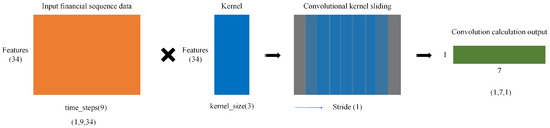
Figure 2.
Conv1D sliding process diagram of financial sequence data.
This describes the sliding computation process of a single convolution kernel, resulting in an output shape of (7, num_filters), representing the extracted features. Thus, after convolution and pooling operations, the final local feature sequence has a shape of (batch_size, new_time_steps, num_filters).
3.1.2. Bidirectional Long Short-Term Memory (BiLSTM)
Bidirectional Long Short-Term Memory (BiLSTM) is a development based on the LSTM model proposed by Hochreiter and Schmidhuber [26]. The concept of a bidirectional recurrent network for processing sequential data was first proposed by Schuster and Paliwal in their 1997 study [27]. BiLSTM combines the hidden states of both forward and backward LSTM networks by simultaneously constructing them, considering both past and future information to generate richer financial indicator sequence features, as shown in Figure 3. Using the local feature representations extracted by the CNN as input, BiLSTM can more comprehensively model the contextual dependencies between financial data points, significantly improving the predictive ability and robustness of the model compared to traditional one-way LSTM.
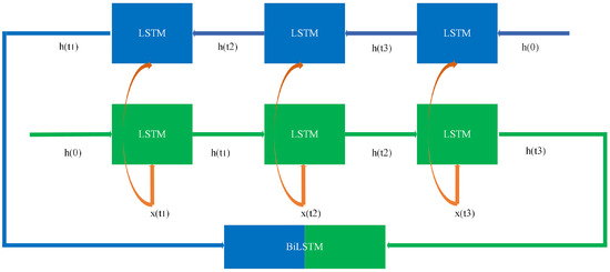
Figure 3.
Structure diagram of BiLSTM.
The local feature sequence extracted by convolution is used as the input of BiLSTM, with a shape of (batch_size, new_time_steps, num_filters). BiLSTM consists of forward LSTM and backward LSTM, and the specific formula is as follows:
where , are the hidden states of forward LSTM and backward LSTM at time step t; , , , are the weight matrix; , are the bias vector. After processing the entire sequence with BiLSTM, the forward and backward hidden states are concatenated to obtain the final temporal feature representation as follows:
The final output shape is (batch_size, new_time_steps, 2 × hidden_size).
3.1.3. Attention Mechanism (AM)
The attention mechanism (AM) was first proposed by Bahdanau et al. in their 2014 study for use in Neural Machine Translation (NMT) tasks [28], enabling the encoder–decoder architecture to dynamically focus on different parts of the input sequence when generating translations, thereby solving the information bottleneck problem of traditional sequence-to-sequence models (Seq2Seq) when processing long sequences. The attention mechanism (AM) focuses on the current time step and dynamically adjusts its weightings based on information from other time steps. The AM enables the model to capture key features across the entire input sequence, enhancing its ability to recognize important temporal dependencies, as shown in Figure 4. We implemented a custom Additive Attention layer to achieve this. The solid lines represent the attention weights at a specific time step (e.g., t = 3), showing how the hidden states are weighted and summed to compute . The dotted lines represent the attention weights at other time steps, illustrating the overall attention mechanism.
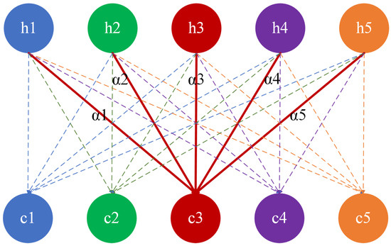
Figure 4.
Structure diagram of an attention mechanism.
The attention mechanism (AM) computes a weighted sum of the hidden states from the BiLSTM, where the attention weights determine how much importance to give to each hidden state. The context vector is the result of this weighted sum. The formula for obtaining the context vector using attention is as follows:
where W is the weight matrix, b is the bias vector, T is the total number of time steps in the input sequence, is the hidden state at time step i, and represents the output context vector for the current time step t.
3.2. Composite Triple Activation Function (CTAF)
The composite triple activation function (CTAF) is systematically designed by integrating two nonlinear activation functions with a multiplicative interaction applied to the raw input tensor x. Formally, it is defined as follows:
where , denote distinct activation primitives (e.g., ReLU, tanh, sigmoid).
The explicit inclusion of the raw input x as a multiplicative component allows the CTAF to retain input signal influence throughout the network. Although it does not constitute a residual connection in the additive sense, the design is partially inspired by the principles underlying residual networks [29] and gradient highway architectures [30], where preserving input pathways improves gradient flow and mitigates vanishing gradients. In a similar spirit, the CTAF promotes effective signal propagation by dynamically modulating the input through dual nonlinear activations. While structurally different, this multiplicative interaction serves a related functional role: maintaining input relevance and enhancing representational diversity, particularly in deeper architectures. The element-wise product ⊙ explicitly couples activation responses, enabling nonlinear feature modulation beyond traditional additive combinations. This interaction dynamically scales feature activations, enhances adaptive gating, and promotes gradient diversity, thus improving representational capacity [31].
In addition, the dual-branch nonlinear transformation enhances feature representation through complementary mechanisms; acts as a sparsity-inducing operator (e.g., ReLU), promoting localized feature selection and suppressing noise, while (e.g., tanh) enforces smooth saturation, ensuring bounded activation ranges to stabilize layer-wise feature magnitudes. From a functional approximation perspective, the multiplicative combination in the CTAF increases the expressiveness of the activation function by expanding the basis function space. Suppose the two nonlinear components and are analytic around 0. They can be expressed using Taylor series as follows:
Then, their product in CTAF becomes
where
This effectively produces a weighted sum of monomials of higher orders, allowing the CTAF to approximate more complex nonlinear mappings. The presence of the input term also shifts the power series upward by one degree, maintaining nonlinearity even when components like ReLU output zero.
Furthermore, the gradient flow through the CTAF can be written as follows:
This expression consists of three gradient-carrying terms. The first term provides a direct gradient signal, even when x is small, and the second and third terms introduce derivative-based modulation, which scales with the input x and preserves sensitivity to local curvature.
This structure is robust; if one component saturates (e.g., tanh), others still transmit gradients. Compared to purely additive or single-branch activations, the CTAF supports multiple gradient pathways. This improves training stability and accelerates convergence. The multiplicative use of the raw input x increases the expressive power of the function, as seen in the Taylor expansion, which produces higher-order monomials. At x = 0, this induces sparsity near zero, which may suppress noise and reduces gradient flow in low-activation regions. As x moves away from zero, nonlinear interactions become stronger. This facilitates gradient flow and avoids the dead neuron problem often seen in ReLU. Overall, the CTAF promotes a more stable and effective learning process by maintaining diverse gradient paths.
3.2.1. Tanh_Relu Activation Function
The tanh_relu activation function can rely on ReLU to accelerate training and feature extraction in positive regions. Leaky ReLU can be used to ensure gradient flow in negative regions, thereby avoiding dead neuron problems. At the same time, tanh maintains smoothness and output centralization, avoiding gradient explosion and improving the convergence and stability of the model. Ultimately, it can effectively improve the learning ability of neural networks when processing complex data, especially in deep networks, helping neurons to better participate in the training process and avoid training stagnation or overfitting.
This function amplifies the considerable value for positive input due to the quadratic growth of . However, the constraint of ensures that its growth will not be too fast, thus helping to maintain numerical stability and avoid gradient explosion. For negative inputs, due to the introduction of the alpha x term, even if x is negative, the output will not be zero, thus avoiding the “dead relu” problem in traditional ReLU networks, where all negative inputs result in zero output. The specific calculation formula and curve graph (Figure 5) are as follows:
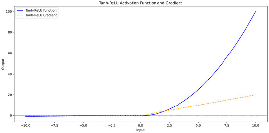
Figure 5.
tanh_relu activation function and gradient curve graph.
3.2.2. Tanh_Sig Activation Function
The tanh_sig activation function combines the strengths of the hyperbolic tangent (tanh) and sigmoid () functions with a scaling factor x. It leverages the smoothness and centralization of tanh(x) to avoid gradient explosion and improve convergence, while (x) introduces nonlinearity and normalization to the range [0, 1]. Including the scaling factor x ensures effective gradient propagation, enabling neurons to better participate in the training process. This combination enhances the learning capacity of neural networks when handling complex data, making it particularly effective for deep networks by preventing stagnation or overfitting.
exhibits symmetry around x = 0, but its output behavior for positive and negative values differs. For x > 0, this function is positive and gradually increases with the increase in x; for x < 0, it is negative and increases when x decreases gradually. Tanh_Sig is continuous and differentiable throughout the entire input space. During backpropagation, the gradient does not suddenly become very large or very small, thus avoiding the risk of gradient explosion or vanishing. The specific calculation formula and curve graph (Figure 6) are as follows:
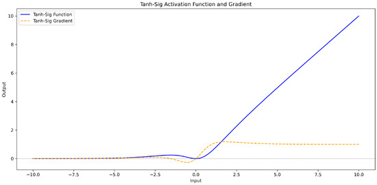
Figure 6.
tanh_sig activation function and gradient curve graph.
3.2.3. Relu_Sig Activation Function
The relu_sig activation function combines the strengths of the Rectified Linear Unit (ReLU) and sigmoid () functions, with an additional scaling factor x. ReLU accelerates feature extraction in the positive region, while Leaky ReLU ensures a small gradient flow in the negative region to prevent the “dead neuron” problem. The sigmoid function smoothens and normalizes the output to the range [0, 1], enhancing nonlinearity. By integrating the scaling factor x, this function improves gradient propagation and feature representation, making it highly effective for complex data processing, particularly in deep networks, by preventing training stagnation and boosting efficiency.
For , as x increases, the output of the function gradually increases, but as the output of the sigmoid function approaches 1, the growth rate will gradually slow down. For x < 0, the function output remains negative, but its absolute value increases with the increase in x. The specific calculation formula and curve graph (Figure 7) are as follows:
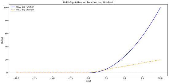
Figure 7.
reLU_sig activation function and gradient curve graph.
4. Experiment
4.1. Overview of Experimental Process
The entire experimental process was divided into five key stages to ensure a systematic exploration and evaluation of the proposed CNN-BiLSTM-AM model optimized with CTAFs. Each stage was designed to build upon the previous one, facilitating the step-by-step optimization and validation of model performance. Figure 8 illustrates the overall workflow.
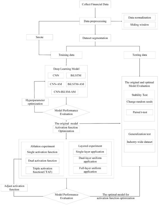
Figure 8.
Experimental process of CNN-BiLSTM-AM model optimized by activation function.
- (1)
- Data Preprocessing: Financial indicator data were collected and preprocessed through normalization and a sliding window approach to convert the raw time series data into structured input samples. We then split the dataset into training and testing sets. To address the class imbalance in the training set, we employed the SMOTE (Synthetic Minority Oversampling Technique), generating synthetic samples for the minority class to ensure balanced training.
- (2)
- Model Construction and Comparison: Multiple deep learning models, including a CNN, BiLSTM, CNN-AM, BiLSTM-AM, and CNN-BiLSTM-AM, were constructed using the training data. These models were evaluated under the same experimental conditions to compare their performance. We conducted hyperparameter optimization to identify the best-performing model architecture.
- (3)
- Activation Function Optimization: CNN-BiLSTM-AM, which was determined to be the optimal structure, was further enhanced through the optimization of the activation function. In this process, we systematically explored different activation function configurations, including single, double, and composite triple activation functions (CTAFs), to evaluate their impact on model performance. In addition, the CTAFs and current activation functions were applied to different layers, such as single-layer, double-layer uniform, and full-layer uniform applications, to examine the influence of layer-by-layer activation distribution. We evaluated the models under each configuration and determined the most effective activation function strategy to improve the model’s nonlinear learning ability.
- (4)
- Stability and Generalization Evaluation: To verify the stability of the optimized model, we conducted additional testing under various conditions. Statistical tests, such as paired t-tests, confirmed the significance of the performance improvements. Additionally, to assess the optimized model’s generalizability, it was tested on a broader industry-wide dataset without industry-specific segmentation.
4.2. Sample Selection
In this study, we investigated 627 manufacturing companies listed on the Shanghai and Shenzhen A-share markets between 2017 and 2024 using data sourced from the CSMAR database. We conducted all experiments using the TensorFlow framework on a Windows 10 operating system.
We included companies only if they had been listed for at least five years, had minimal missing data, and had maintained continuous quarterly financial records for the most recent 12 quarters to ensure data integrity and consistency. The dataset was divided into two groups:
- (1)
- ST companies, which were initially designated as “Special Treatment” (ST) due to abnormal financial conditions, such as two consecutive years of losses.
- (2)
- Non-ST companies, which remained financially stable and were not marked for ST designation during the observation period. To ensure comparability between the two groups, non-ST companies were selected from the same industry and year as the ST companies, with comparable asset scales (within ±20%) and no ST designation in that year.
In this study, we used 12 quarters of financial indicators from year T-5 to T-3 (where T is the year that a company was first marked as ST) as input features, aiming to enable early financial risk prediction and capture warning signals prior to financial distress.
The sample distribution is shown in Table 2. The total number of company samples was 627, and the total number of time series data points across 12 quarters was 7524.
Table 2.
Sample distribution table.
4.3. Indicator Selection
This study used seven categories of indicators to evaluate financial performance, including 34 indicators in total. These categories included debt-paying ability, ratio structure, operating ability, profitability, cash flow ability, development ability, and per-share indicators. Collectively, these indicators provide a comprehensive analysis of a company’s financial and risk status.
These indicators can be categorized into seven categories:
- (1)
- Debt-paying ability, including current ratio, quick ratio, cash ratio, working capital, debt-to-asset ratio, equity multiplier, and equity ratio;
- (2)
- Ratio structure, including current assets ratio, cash assets ratio, working capital ratio, non-current assets ratio, current liabilities ratio, fixed assets ratio, and operating profit margin;
- (3)
- Operating ability, including accounts receivable turnover, inventory turnover, accounts payable turnover, current asset turnover, fixed asset turnover, and total asset turnover;
- (4)
- Profitability, including return on assets, net profit margin on total assets, net profit margin on current assets, net profit margin on fixed assets, return on equity, and operating profit rate;
- (5)
- Cash flow ability, including the operating index;
- (6)
- Development ability, including capital preservation and appreciation rate, fixed asset growth rate, revenue growth rate, sustainable growth rate, and owners’ equity growth rate;
- (7)
- Per share, including earnings per share and earnings before interest and taxes per share.
The box plot of the key financial indicators in Figure 9 reveals that ST enterprises face substantial financial challenges compared to non-ST enterprises. These include insufficient short-term debt-paying ability (low cash ratio, cash assets ratio, current ratio, and quick ratio), high debt burden (high debt to asset ratio, current liabilities ratio and equity multiplier), and weak profitability (low operating profit rate). Additionally, ST enterprises show lower growth potential (low fixed asset growth rate) and reduced asset flexibility (high fixed assets ratio).
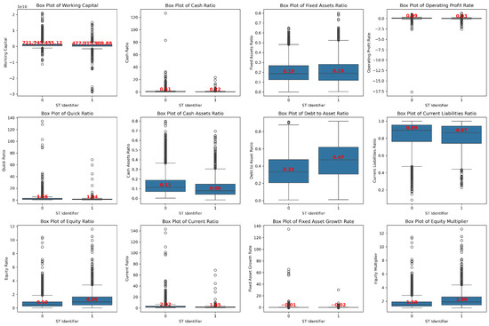
Figure 9.
Box plot of the main financial indicators.
4.4. Data Preprocessing
4.4.1. Sliding Window
For this study, we selected the time series data of financial indicators from each company over the past 12 quarters, with 1380 time series points for ST manufacturing companies and 6144 time series points for non-ST companies. In order to better utilize these time series data, we adopted the sliding window technique, where the data slide on the time series with a fixed window size. Each window contains financial data for several consecutive time steps, generating multiple overlapping time series samples. In a study on Internet financial credit risk prediction, Li et al. [32] combined the sliding window technique with the attention mechanism LSTM model and empirically verified its effectiveness and practicability in financial time series modeling. The sliding window technique is a commonly used method for time series modeling and sample expansion; it can divide long sequences into multiple overlapping short sequences, enhance the model’s ability to learn local dynamic features, and improve generalization performance.
Specifically, given a time series , , ⋯, , with a window size of w, it is possible to generate samples. Each sample consists of a sub-sequence of length w, represented as ..., where .... Each sub-sequence is associated with a corresponding label y.
In this study, the specific implementation method is as follows:
Each company provides data for 12 quarters assuming that the number of sliding windows is 8. During the sliding process, the window moves backward by one time step each time, containing financial indicators for eight consecutive time steps as feature data (X). It is important to note that the target value y for all samples generated by each company remains consistent and corresponds to the company’s ST status.
Sample 1: → Objective: Identifier (Company);
Sample 2: → Objective: Identifier (Company);
Sample 3: → Objective: Identifier (Company);
Sample 4: → Objective: Identifier (Company);
Sample 5: → Objective: Identifier (Company).
When the sliding window size is 8, the number of samples that each company can generate is 12 − 8 + 1 = 5. If the total number of companies is n, the sample size is 5 × n.
In this study, a ratio of 7:3 was set for the training and testing sets. The distribution of the sliding window samples is shown in Table 3. As the sliding window size decreases from w = 12 to w = 4, the total number of samples in the training and testing sets significantly increases. The number of non-ST and ST samples grows synchronously.
Table 3.
Distribution of sliding window samples.
4.4.2. SMOTE Oversampling
The raw data show a significant sample imbalance between ST manufacturing companies and non-ST companies, which may cause the model to lean towards categories with a larger sample size during training. This study adopted the Synthetic Minority Oversampling Technique (SMOTE), a well-established method proposed by Chawla, to address this issue and balance the class distribution [33]. Unlike random oversampling, which duplicates existing samples and may cause overfitting, the SMOTE generates synthetic samples by interpolating between minority class samples, thereby enriching the decision boundary and improving model generalization.
Specifically, the SMOTE works as follows: (1) It randomly selects a minority class sample as the reference point; (2) it finds the k-nearest neighbors of within the minority class; (3) based on a sampling ratio N%, it randomly selects neighbors ; and (4) it creates new synthetic samples by linearly interpolating between and . This approach helps to expand the feature space coverage of the minority class without introducing noise or redundancy.
The SMOTE alleviates the class imbalance by generating composite samples, specifically by interpolating the composite data points of minority-class samples to increase the number of minority-class samples. By applying the SMOTE to the training set and oversampling minority class samples, the class distribution in the training data is balanced, thereby improving the model’s fairness and generalization ability.
In this study, the SMOTE was applied only to the training set to avoid data leakage. Taking a time step of 8 (w = 8) as an example, in the original training data, the sample size of ST companies is 410, and the sample size of non-ST companies is 1797 ( Table 3). The synthesized samples generated by the SMOTE increase the number of ST company samples from 410 to 1797, which is equal to the number of non-ST company samples (as shown in Figure 10). This process effectively increases the sample size of minority classes (ST companies), significantly improving the data balance and reducing the bias caused by the class imbalance.
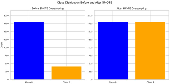
Figure 10.
Comparison of training set data before and after the SMOTE (w = 8).
5. Results
5.1. Model Construction and Comparison
A series of experiments was conducted using the same dataset for both training and evaluation to compare the effects of different model structures and time steps. In the CNN-BiLSTM-AM model, all components are combined to improve feature extraction and long-term learning. In addition, the CNN layer defaults to the ReLU activation function, the BiLSTM layer defaults to tanh as the primary activation function, and the Dense layer defaults to the ReLU activation function. These configurations help in assessing the impact of each layer on performance.
The CNN-BiLSTM-AM model’s hyperparameters were optimized using a grid search strategy over predefined search ranges (Table 4). This exhaustive search method allowed for a systematic evaluation of all possible combinations of hyperparameters to identify the configuration yielding the best model performance [34]. Table 4 presents the search ranges and the optimal values identified during the tuning process.
Table 4.
Optimal hyperparameter configuration.
Table 5 details the various model structures with different CNN, BiLSTM, and attention layer combinations. The CNN model captures local features, while an attention layer is incorporated into the CNN-AM model to focus on key features. The BiLSTM model learns long-term dependencies, and an attention layer is incorporated into the BiLSTM-AM model to enhance its performance. To compare the impact of different layers on the results, the hyperparameter settings of other selected model architectures were set to be consistent with those of CNN-BiLSTM-AM.
Table 5.
Different model structure tables.
5.1.1. Prediction Results of Different Models at Different Time Steps
The prediction results of the different models at various time steps show significant performance changes as the time step decreases from 12 to 4. As shown in Table 6, the CNN-BiLSTM-AM model tends to provide the best results across all time steps. At a time step of w = 8, the CNN-AM, BiLSTM, BiLSTM-AM, and CNN-BiLSTM-AM models perform best, while the CNN model performs best at w = 6.
Table 6.
Prediction results of different models at different time steps.
5.1.2. Comparison of Different Model Results at w = 8
Figure 11 illustrates the models’ performance at a specific time step (w = 8), highlighting the impact of different architectures. It presents the overall accuracy, recall, and F1-score for predicting ST companies. The accuracy of the CNN model is 95.1%, while that of the CNN-AM model with an attention mechanism is significantly improved to 98.7%. The accuracy of the BiLSTM model is 96.9%, slightly higher than that of the CNN but still lower than that of CNN-AM. The accuracy of the BiLSTM-AM model with an attention mechanism is 98.6%, outperforming that of BiLSTM and approaching that of CNN-AM. The CNN-BiLSTM-AM model, in which a CNN, BiLSTM, and an AM are combined, performs the best, with an accuracy of 98.8%. Overall, the introduction of an attention mechanism effectively improves the performance of the CNN and BiLSTM, with the CNN-BiLSTM-AM architecture performing the best under this setting.
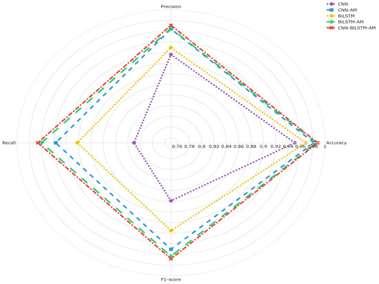
Figure 11.
Comparison of results from different models.
According to the ROC curve and the AUC value in Figure 12, it has the best performance and can perfectly distinguish between positive and negative samples. The AUC of the CNN model is 0.96, indicating a relatively weak discriminative ability, while that of the CNN-AM model with an added attention mechanism is improved to 0.98, demonstrating a strong classification ability. The AUC values of BiLSTM and BiLSTM-AM are 0.98 and 0.99, respectively, with the performance of the latter further improving as a result of the introduction of an attention mechanism. Overall, adding an attention mechanism significantly improves the predictive ability of the models, especially that of BiLSTM-AM and CNN-AM.
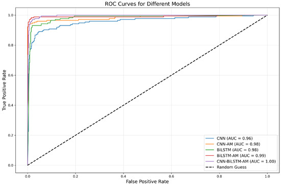
Figure 12.
ROC curves for different models.
5.1.3. Feature Importance Analysis of the CNN-BiLSTM-AM Model
To further interpret the prediction results of the optimal model CNN-BiLSTM-AM, permutation importance was employed to evaluate the contribution of each input feature [35]. This method measures the decrease in model performance when the values of a specific feature are randomly shuffled, thereby allowing for an assessment of how much the model relies on each feature for prediction.
As shown in Figure 13, the most influential features, including total asset turnover, return on assets, cash assets ratio, working capital, and earnings before interest and taxes per share, caused the most significant decline in model performance when permuted. This indicates that the CNN-BiLSTM-AM model relies heavily on these variables for accurate classification. In contrast, features such as capital preservation and appreciation rate, fixed asset growth rate, operating profit margin, accounts receivable turnover, and operating index exhibited relatively low importance scores, suggesting a limited contribution to the model’s predictions. This analysis enhances the interpretability of the CNN-BiLSTM-AM model. The results confirm that the model’s decision-making process aligns with financial indicators widely recognized as significant within the domain.

Figure 13.
Permutation feature importance of the CNN-BiLSTM-AM model.
5.2. Comparison of CNN-BiLSTM-AM Results Under Different Activation Functions
5.2.1. Ablation Experiment Results
Next, we designed a layer-wise activation function ablation study to systematically evaluate the impact of activation functions on model performance across different network layers. Using “CNN-ReLU, BiLSTM-Tanh, Dense-ReLU” as the benchmark model structure, only one activation function layer is replaced in each round of experiments. In contrast, the other two layers remain unchanged, effectively avoiding the interference of multivariate coupling in the result analysis, thus ensuring the comparability of the experiments and the reliability of the conclusions.
Through this experiment, we systematically investigated a range of activation functions and their combination forms, including tanh, relu, x, xtanh, xrelu, tanhrelu, and tanh_relu, by performing layer-wise substitutions in the CNN-BiLSTM-AM model. This ablation design aimed to assess the influence of each activation variant on classification accuracy. More importantly, it validated the superiority of the proposed composite triple activation function (CTAF) over conventional single or composite double activation functions. By comparing performance across different configurations, this experiment provided strong empirical support for the effectiveness and adaptability of the CTAF mechanism. Table 7 and Table 8 show the ablation experiment design and activation function description.
Table 7.
Activation function settings for different layer change strategies.
Table 8.
Activation function combinations and formulas.
1. Ablation Results of Activation Function Variants in the CNN Layer
In the CNN layer, the experimental results (Figure 14) obtained after replacing different activation functions show that the CTAF (tanh_relu) configuration achieves the highest accuracy of 0.993, significantly better than that of traditional single functions (such as relu, with a value of 0.988, and tanh, with a value of 0.991) and some composite variants (such as xtant and xrelu, both with a value of 0.984). This confirms that, in the convolutional feature extraction stage, integrating multiple nonlinear transformations can effectively improve the expressive power of the model, especially compared to sigmoid activation (which is quickly saturated and has an accuracy as low as 0.965), which has more advantages.
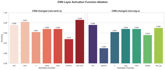
Figure 14.
Ablation results of activation function variants in the CNN layer.
2. Ablation Results of Activation Function Variants in the BiLSTM Layer
In the BiLSTM layer, the experimental results (Figure 15) show that the tanh activation function (0.988 accuracy) in the original configuration is still optimal. At the same time, alternative solutions, such as relu, xrelu, and tanhrelu, were explored but did not achieve better results, with the highest value being only 0.986. Due to there being multiple tanh/sigmoid-based gating mechanisms in the BiLSTM architecture, modifying the activation function can easily compromise its gradient stability and time modeling capabilities. Therefore, this layer is more sensitive to the activation function, and retaining the standard tanh is more conducive to temporal dependency modeling.
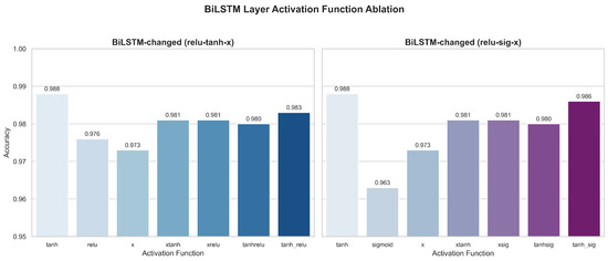
Figure 15.
Ablation results of activation function variants in the BiLSTM layer.
3. Ablation Results of Activation Function Variants in the Dense Layer
In the Dense layer, the baseline relu accuracy is 0.988, which improves to 0.991 when using xtanh and the CTAF (tanh_relu). This indicates that introducing composite activation in the feature integration stage helps enhance the decision-making ability. However, not all combinations are effective. For example, the accuracy of xrelu and tanhrelu decreases to 0.983 (Figure 16), indicating that the synergistic effect between functions significantly impacts the results and that caution must be taken with combination design.

Figure 16.
Ablation results of activation function variants in the Dense layer.
Overall, the ablation results demonstrate the advantages of the CTAF in specific layers (especially the CNN and Dense layers), further indicating that activation strategies should be flexibly adjusted based on differences in network layer functionality.
5.2.2. Layered Experiment Results
The aim of this study was to comparatively analyze the impact of the composite triple activation function (CTAF) and several commonly used activation functions on model performance across different layers. We explored the following three strategies, as shown in Figure 17, in order to minimize interference from multi-layer structures and ensure experimental validity:
- (1)
- Activation Strategies in the BiLSTM LayerTwo fine-grained strategies adapted specifically for the BiLSTM layer were used to further investigate how activation functions influence sequence modeling:
- (i)
- Direct replacement of the BiLSTM main activation function: The default main activation function (usually tanh) in the BiLSTM layer is modified, and its impact on sequence feature extraction and overall model performance is observed.
- (ii)
- Post-processing activation via Lambda layer: After the BiLSTM layer output its results, the model applies the activation function through a Lambda layer while keeping the BiLSTM layer’s default activation function unchanged. Then, it adds a Lambda layer after its output and performs further nonlinear transformations on the output (applying activation functions) to achieve finer control.
- (2)
- Activation Function Deployment Strategies Across Network Layers
- (i)
- Single-layer application: A specific activation function is applied to only one single layer, keeping the other layers unchanged. This isolates the influence of each activation function within a single network component.
- (ii)
- Dual-layer uniform application: The same activation function is applied to both the CNN and flattened Dense layers while varying the activation function in the BiLSTM or BiLSTM-Lambda layer. This setup allows for an evaluation of how the recurrent layer interacts with fixed nonlinear transformations in the non-recurrent layers and how this affects overall model performance.
- (iii)
- Full-layer uniform application: The same activation function is uniformly applied across all key layers. This strategy allows for an evaluation of the global effect of consistent nonlinearity throughout the network hierarchy.

Figure 17.
Optimization of activation function structure in different layers of CNN-BiLSTM-AM model.
Figure 17.
Optimization of activation function structure in different layers of CNN-BiLSTM-AM model.
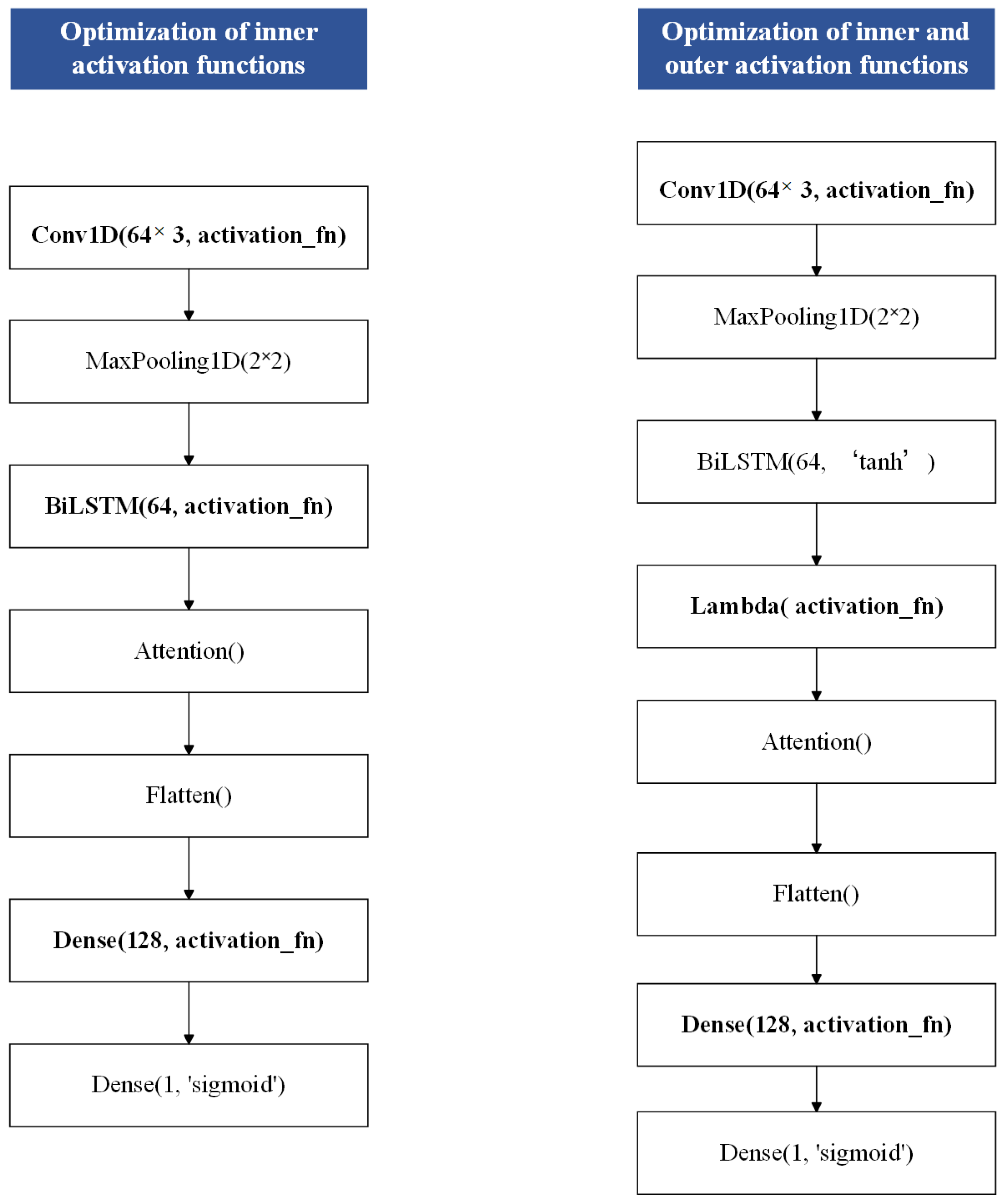
By comparing these strategies with the CTAF and widely used activation functions (e.g., relu, tanh, sigmoid, swish, mish, and leaky relu) and evaluating the application positions and mechanisms of activation functions, the impacts of activation functions on sequence modeling and feature expression were further revealed. In addition, in the experimental design, other hyperparameters and structural configurations were controlled consistently to ensure the comparability of the experimental results and the validity of the conclusions.
1. Single-Layer Activation Function Comparison
In this section, we investigate the effect of applying different activation functions to a single network layer (the CNN, BiLSTM, BiLSTM-Lambda, or Dense layers) while keeping the remaining layers unchanged. The purpose of this is to isolate and observe how each activation function independently influences model learning and performance within a specific layer.
Table 9 compares the classification accuracy of different activation functions applied to individual layers (the CNN, Dense, BiLSTM, and BiLSTM with Lambda activation layers). The results show that the activation function choice significantly affects model performance across layers.
Table 9.
Single-layer activation functions comparison.
In the CNN layer, CTAFs such as tanh_sig (0.993) and tanh_relu (0.993) outperform standard functions such as relu (0.988) and tanh (0.984), while sigmoid shows the lowest performance (0.965), likely due to gradient vanishing issues.
In the Dense layer, CTAFs such as tanh_relu (0.991) and swish (0.989) achieve the highest accuracy, indicating that smoother or composite functions improve classification performance. Traditional functions such as sigmoid and leaky relu perform worse (≤0.981).
In the BiLSTM layer, tanh (0.988) remains a strong performer, while sigmoid again lags (0.964). After applying activation functions through a Lambda layer post-BiLSTM, the performance of tanh and tanh_relu increases to 0.993, suggesting that post-processing with nonlinearities enhances sequential feature representation.
Overall, the results highlight the effectiveness of CTAFs and the potential of BiLSTM-Lambda nonlinear transformation to enhance model performance.
2. Dual-Layer Activation Function Comparison
In this section, we investigate how the interaction between the activation functions applied to the CNN and Dense layers and those applied to the BiLSTM or BiLSTM-Lambda layer affects model performance. Specifically, two directions are explored: (1) fixing the CNN and Dense layers while varying the activation functions in the BiLSTM or BiLSTM-Lambda layer and (2) fixing the BiLSTM or BiLSTM-Lambda layer while uniformly applying activation functions to both the CNN and Dense layers.
According to Table 10, the model uses the CTAF tanh_sig in the CNN and Dense layers. In contrast, the BiLSTM layer maintains the default activation function tanh, improving the accuracy from 0.988 to 0.990, which is the optimal combination. Secondly, when using leaky relu in the CNN and Dense layers and tanh in the BiLSTM layer, when using tanh in the CNN and Dense layers and tanh_relu in the BiLSTM layer, or when using mish in the CNN and Dense layers and tanh in the BiLSTM layer, the accuracy reaches 0.989. The BiLSTM layer performs more stably when using the main tanh activation function.
Table 10.
Dual-layer and BiLSTM layer activation functions comparison.
Due to the slight improvement in model performance caused by directly changing the default activation function of the BiLSTM layer, we further attempted to apply activation functions to the output data of the BiLSTM layer through the Lambda layer. According to Table 11, when the model uses the tanh activation function in the Dense layer after the CNN and flattening layers and applies the CTAF tanh_relu in the Lambda layer after the BiLSTM layer output, the accuracy improves from 0.988 to 0.995, showing the best performance. Secondly, when using the relu activation function in the CNN and Dense layers, combined with the CTAF relu_sig or tanh_sig in the Lambda layer, the accuracy reaches 0.992 and 0.990, respectively.
Table 11.
Dual-layer and BiLSTM-Lambda layer activation functions comparison.
Overall, the model achieves significantly better performance when applying the BiLSTM layer outputs and CTAFs (such as tanh_relu, relu_sig, and tanh_sig) through the Lambda layer than when using traditional activation functions or existing combinations of extended activation functions. This indicates that further nonlinear transformation of the output data of the BiLSTM layer can improve the model’s feature expression ability and prediction performance.
3. Full-Layer Activation Function Comparison
In this section, we explore how uniformly applying the same activation function across all key network layers, including the CNN, BiLSTM (or BiLSTM-Lambda), and Dense layers, impacts performance. By applying identical activation functions throughout the model, the goal was to evaluate how unified nonlinear transformations influence end-to-end feature learning and model generalization.
As shown in Table 12, under the strategy of a unified activation function, the overall performance of the model structure improves after adding the Lambda layer (CNN-BiLSTM-Lambda-Dense), and the accuracy of almost all activation functions is higher than that of the CNN-BiLSTM-Dense structure without the Lambda layer. For example, relu increases from 0.976 to 0.990, tanh increases from 0.989 to 0.993, and mish increases from 0.988 to 0.992, showing stable and excellent performance. However, the CTAFs do not achieve high accuracy in both structures, indicating their poor performance and limited applicability when applied uniformly throughout the entire layer.
Table 12.
Full-layer activation functions comparison.
To summarize, in this study, we systematically analyzed the impact of activation functions on performance at different levels of deep model applications. The results show that a CTAF could significantly improve model performance when applied to the CNN, Dense, and Lambda layers after BiLSTM outputs, with an accuracy of up to 0.995 achieved when using specific combinations (when using tanh in the CNN and Dense layers and tanh_relu in the Lambda layer after BiLSTM). The BiLSTM layer remains stable when using traditional tanh functions, and introducing nonlinear transformations through the Lambda layer further improves its performance. The overall performance of the strategy of applying the same CTAF uniformly to all layers is poor, indicating that the activation function should be tailored to different layer structures. Adopting a targeted activation function layout, especially combining CTAFs and Lambda structures, helps to enhance the model’s feature expression ability and prediction accuracy.
5.3. Performance of CNN-BiLSTM-AM Model with CTAF
5.3.1. Comparison of Performance of the Original and Optimal Models
By optimizing a combination of activation functions (CNN and Dense layers: tanh; Lambda layer after BiLSTM output: tanh_relu), the model achieves optimal performance with an accuracy of up to 99.5%. Figure 18 shows that the accuracy and loss value curves of the model tend to be stable, indicating that the model exhibits good convergence and stability during the training process and has strong robustness.
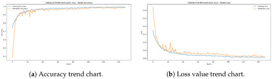
Figure 18.
The accuracy and loss trend chart of the optimal model.
In this study, relu was used as the original activation function in the CNN and Dense layers, and tanh was used in the BiLSTM layer. Then, tanh was used as the optimized activation function in the CNN and Dense layers, tanh was used in the BiLSTM layer, and the CTAF tanh_relu was used in the Lambda layer. Performance comparisons between the original and optimized configurations demonstrate significant improvements, with the overall accuracy increasing from 98.8% to 99.5%. As shown in Figure 19 and Figure 20, the key performance enhancements include the following:
- (1)
- Non-ST Company Recall: Increased from 97.1% to 100%, correctly identifying all 772 non-ST companies without omission, demonstrating improved recognition of majority-class samples.
- (2)
- ST Company Accuracy: Improved from 99.4% to 100%, indicating no false positives among the 169 predicted ST companies.
- (3)
- ST Company Recall: Increased from 96.6% to 97.1%, reducing missed ST identifications from six to five among 174 true ST samples.

Figure 19.
Comparison of precision and recall between original and optimal activation functions.
Figure 19.
Comparison of precision and recall between original and optimal activation functions.
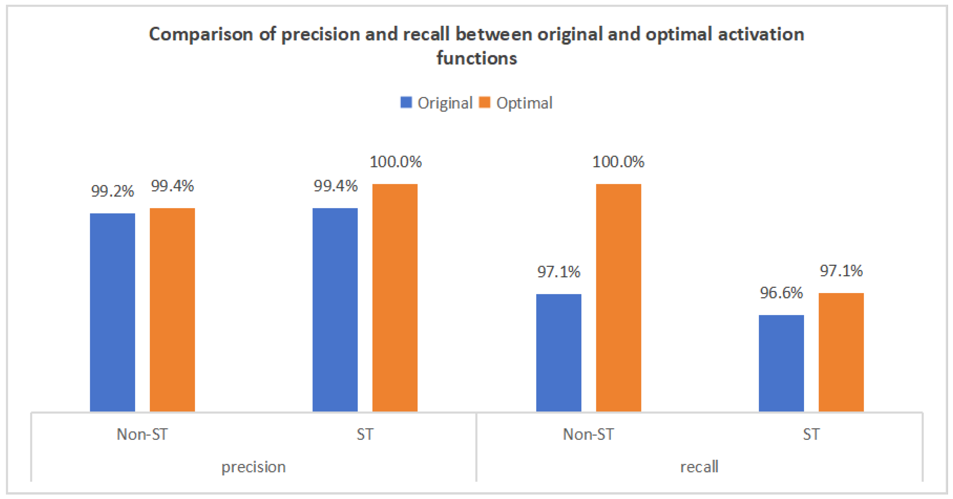

Figure 20.
Comparison of confusion matrices between original and optimal activation functions.
Figure 20.
Comparison of confusion matrices between original and optimal activation functions.
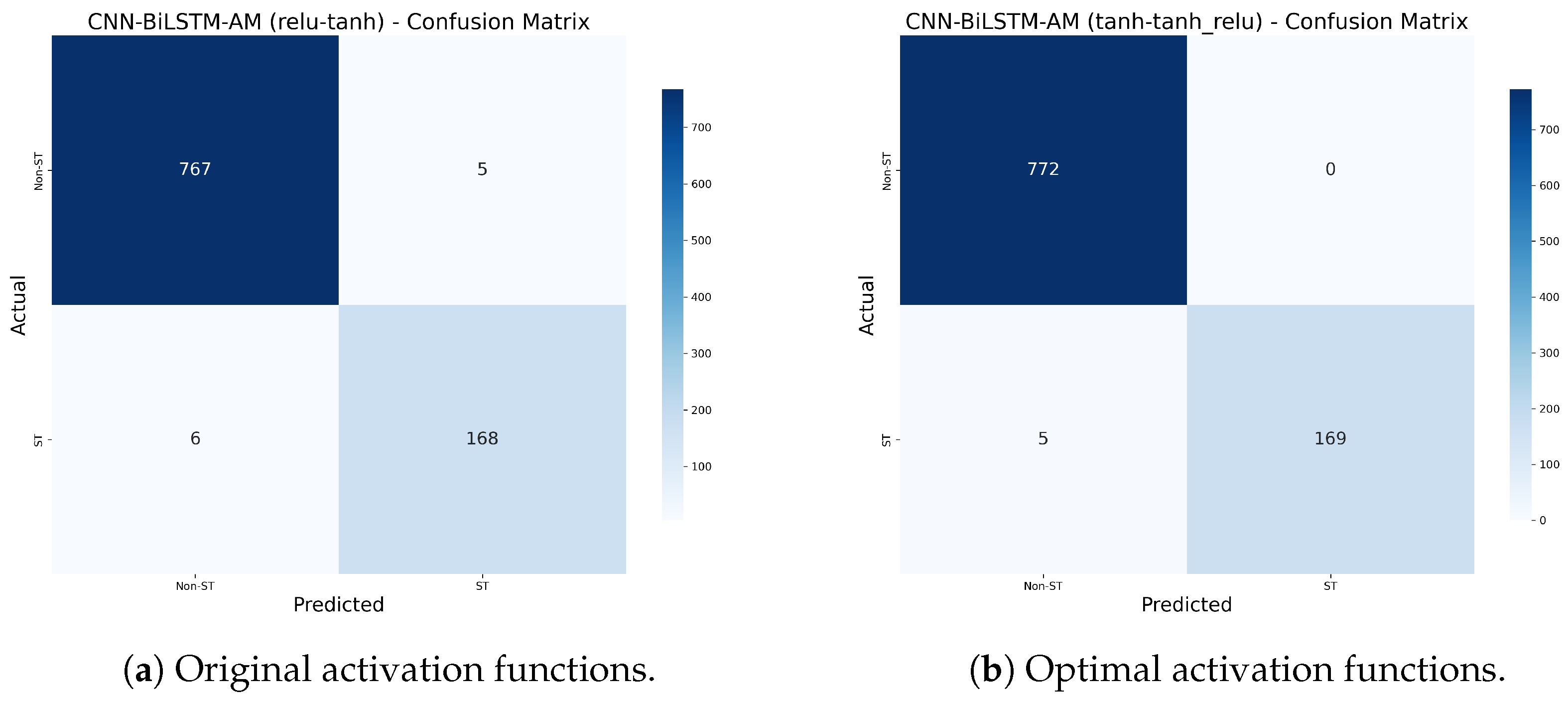
These results confirm that the optimized activation function configuration enhances accuracy and class balance. The model shows improved robustness, particularly in identifying minority-class (ST) samples, validating the effectiveness of activation function optimization in addressing class imbalance.
5.3.2. Stability Test Between the Original and Optimal Models
To ensure a fair comparison of different activation function combinations under the same parameter settings and dataset configuration, we initially set a fixed random seed (42) to guarantee result reproducibility. To further eliminate the possibility of performance improvements being due to randomness, both the original and optimized models were trained and evaluated 20 times with different random seeds. Figure 21 and Figure 22 show the accuracy trend and box plot distribution of the two models. The results show that the optimized model consistently outperforms the original model.
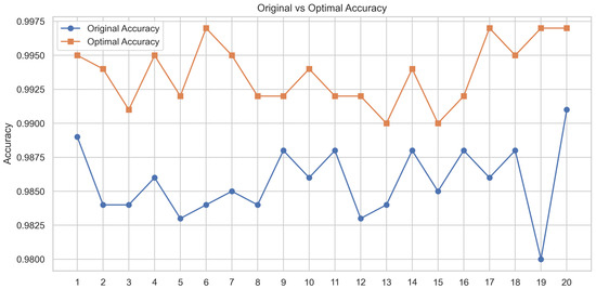
Figure 21.
Accuracy trend chart of the original model and optimal model in random experiments.
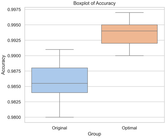
Figure 22.
Accuracy box plot of the original and optimal models in random experiments.
As shown in Table 13, the results of these 20 experiments were first subjected to a normality test using the Shapiro–Wilk test, which confirmed that the data followed a normal distribution (p = 0.067). We conducted a paired t-test, which revealed a statistically significant difference between the two models (t = −10.932, p < 0.001). These findings demonstrate that the proposed CTAF optimal model consistently demonstrates significant performance improvements across random conditions.
Table 13.
Statistical test results.
5.3.3. Generalization Test Between the Original and Optimal Models
The comparison between the original and optimized models was extended to an industry-wide dataset to assess the practical significance and generalizability of the proposed activation function optimization. This dataset includes ST and non-ST companies across all industries, comprising 890 companies and 10,680 time series samples. We conducted data preprocessing using the same approach, including a sliding window technique and SMOTE oversampling. With the time step set to 8, we evaluated the original and optimized models under consistent experimental settings.
As shown in Figure 23, the optimized model achieves an accuracy of 99.4%, outperforming the original model’s 98.9%. In particular, the recognition performance for ST companies improves significantly. Additionally, Figure 24 shows that the optimized model’s ROC curve demonstrates superior overall classification capability. These findings further validate the robustness and practical applicability of the optimized activation function (CTAF) design across diverse industry scenarios.
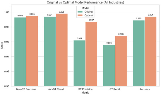
Figure 23.
Comparison of performance between original and optimal models across industries.
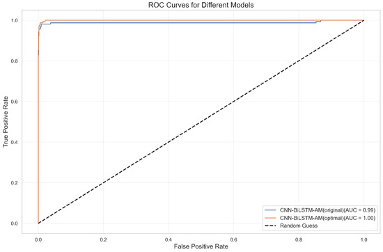
Figure 24.
ROC curves for original and optimal models across industries.
5.4. Summary of Results
Employing the experimental results presented in this section, we conducted a detailed performance evaluation of CNN BiLSTM-AM and the optimized CTAF. The main results are as follows:
- (1)
- Model construction and comparison: When the time step is w = 8, CNN-BiLSTM-AM achieves the best performance (0.988), outperforming the other models.
- (2)
- Comparison of CNN-BiLSTM-AM results under different activation functions: In the ablation and layered experiments, the CTAF shows the best application effect in the single-layer CNN, Dense layer, and Lambda layer, with corresponding model accuracies of 0.993, 0.991, and 0.993, respectively. However, in the BiLSTM layer, the performance of the CTAF is poor, and the original tanh activation function performs better. When the CNN, BiLSTM, and Dense layers use tanh and the CTAF (tanh_relu) is applied in the Lambda layer after BiLSTM, the model’s accuracy reaches its highest level (0.995). However, the model performance decreases when the CTAF is applied to all layers.
- (3)
- Performance of CNN-BiLSTM-AM model with the CATF: The paired t-test and industry-wide data expansion experiment verify that the optimal model consistently outperforms the original model.
6. Conclusions
6.1. Research Conclusions
This study proposes a CNN-BiLSTM-AM deep learning model based on CTAF optimization for predicting the financial risks of listed manufacturing companies using 12-quarter time series financial indicator data. An empirical analysis shows that the model and its optimization strategy have significant effectiveness and practical value. The main research conclusions are as follows:
- (1)
- The comprehensive advantages of the CNN-BiLSTM-AM model: Under the default activation function configuration, the predictive performance of the CNN-BiLSTM-AM model is superior to that of single or partial combination models such as CNNs, CNN-AM, BiLSTM, and BiLSTM AM, with an optimal accuracy (98.8%) and AUC value (1.00). This indicates that the model effectively combines the local feature extraction ability of the CNN, the temporal modeling ability of BiLSTM, and the feature selection ability of the attention mechanism, demonstrating excellent prediction performance.
- (2)
- The effectiveness of the attention mechanism: Introducing an attention mechanism significantly enhances the model’s ability to select key features. A comparative analysis shows that models with attention mechanisms, such as CNN-AM and BiLSTM-AM, perform significantly better in terms of accuracy and AUC values than models without attention mechanisms, further confirming the important role of attention mechanisms in modeling complex temporal data.
- (3)
- The identification of key financial indicators: Using permutation importance, it is found that the CNN-BiLSTM-AM model relies mostly on key financial indicators such as total asset turnover, return on assets, cash assets ratio, working capital, and earnings before interest and taxes per share, as permuting these indicators causes the most significant drop in performance.
- (4)
- Layer-wise ablation validates the superiority of the CTAF: Through structured ablation and comparative experiments involving single activation functions (e.g., relu and tanh), dual combinations (e.g., tanhrelu), and composite triple activation functions (CTAFs, e.g., tanh_relu), the proposed CTAF demonstrates clear performance advantages. Particularly in the CNN and Dense layers, the CTAF (tanh_relu) consistently achieves the highest accuracy, highlighting its superior nonlinear feature extraction and gradient propagation capabilities. Even in the BiLSTM layer, which is sensitive due to its gating mechanisms, the CTAF maintains competitive stability, confirming its generalizability across different layer types.
- (5)
- Activation functions exhibit heterogeneous performance in different network layers: The experimental results show that composite triple activation functions (CTAFs) are particularly effective in the CNN and Dense layers, where deep feature extraction and nonlinear decision boundaries are essential. In contrast, recurrent layers such as BiLSTM achieve better stability and performance with traditional tanh, benefiting from its balanced gradient flow and temporal memory capabilities. Furthermore, applying CTAFs in a Lambda layer after the BiLSTM output enhances sequential feature representation, revealing that activation efficiency is not only layer specific but also influenced by positional deployment within the architecture.
- (6)
- Significant effect and stability of the CTAF: The optimized model achieves the best performance when using tanh in the CNN and Dense layers and the CTAF tanh_relu in the Lambda layer after the BiLSTM output, increasing the accuracy from 98.8% to 99.5%. Repeated experiments under 20 random seeds confirmed that the improvement is stable and statistically significant (paired t-test), verifying both the effectiveness and robustness of the CTAF.
- (7)
- The CTAF demonstrates robust generalizability across industries: The effectiveness of the proposed composite triple activation function (CTAF) is not limited to the manufacturing sector. When applied to an industry-wide dataset covering a diverse set of ST and non-ST companies, the optimized model maintains superior performance, improving accuracy from 98.9% to 99.4%. The enhanced recognition of ST companies and improved ROC characteristics confirm that the CTAF retains its predictive advantages in broader real-world scenarios.
6.2. Discussion
6.2.1. Discussion of Model and CTAF Validity
The empirical results indicate that the CNN-BiLSTM-AM model optimized with a composite triple activation function (CTAF) effectively predicts financial risks in the manufacturing industry. This model’s advantage comes from its integrated design; the CNN layer extracts local spatial patterns from multivariate financial time series, the BiLSTM layer captures complex temporal dependencies, and the attention mechanism highlights key time steps related to risk prediction.
The important innovation of this study lies in the introduction of a composite triple activation function (CTAF), which enhances the model’s ability to learn nonlinear relationships by combining multiple activation functions (such as tanh and relu), particularly achieving significant performance improvements in the CNN and Dense layers. Compared with traditional activation strategies such as ReLU or tanh alone, the CTAF provides a more flexible and complex nonlinear mapping in a multi-level feature structure, which can more fully express the implicit risk features in financial data. In addition, deploying the CTAF through the Lambda layer after the BiLSTM layer not only maintains the memory characteristics of the recurrent neural network (RNN) for the time series but also introduces new nonlinear transformations, significantly improving the model’s discriminative ability at the end of the sequence. This layered deployment strategy enhances the nonlinear flow and depth of information expression in the network, which helps to construct more stable and generalizable discriminative boundaries.
These findings emphasize that activation function optimization, which is often overlooked in financial deep learning, can significantly improve model performance. A CTAF provides empirical improvements and offers a balanced gradient flow, feature representation, and generalization method.
6.2.2. Practical Implications and Application of the Model
The CNN-BiLSTM-AM model optimized using a CTAF can be effectively embedded in the financial warning system of manufacturing enterprises to actively identify the early signs of financial distress. By utilizing quarterly time series financial indicators, this model can be used to dynamically monitor the company’s financial situation, provide timely alerts, and support risk prevention and strategic planning.
In addition, identifying high-impact financial features and combining them with a permutation importance analysis can improve the interpretability of the model. Manufacturing companies can use this information to prioritize internal evaluations and optimize the management of these indicators. The risk management team can develop targeted intervention strategies based on specific indicators marked by the model, such as improving operational efficiency or adjusting capital structure. This will help them to move from passive financial reporting to proactive, data-driven financial governance, enhancing the overall resilience of enterprises in volatile market environments.
6.2.3. Research Limitations and Plans
Although the CTAF-optimized CNN-BiLSTM-AM model shows strong performance, several limitations remain. The model does not consider external factors such as macroeconomic conditions and industry competition, often crucial in real-world financial risk prediction. It also overlooks unstructured data sources such as financial news and company reports, limiting its ability to capture broader risk signals. In addition, the selection and placement of activation functions across the four layers remain based on empirical design, as we did not systematically explore all possible combinations.
Future research could integrate external indicators and unstructured data to improve the model’s comprehensiveness and applicability. Automated tools such as neural architecture search (NAS) could be employed to optimize activation function configurations more systematically. Exploring adaptive activation functions may also provide greater flexibility and enhanced performance. Furthermore, incorporating advanced architectures such as graph neural networks (GNNs), Transformer-based models, and multimodal data fusion techniques can help improve prediction accuracy and robustness. These developments will support the construction of intelligent, interpretable, and sustainable financial risk early warning systems, offering long-term value to enterprises and decision-makers in managing complex financial environments.
Author Contributions
Conceptualization, P.B.; methodology, P.B.; software, Y.S.; validation, Y.S. and M.C.; formal analysis, P.B., Y.S. and M.C.; investigation, P.B.; resources, Y.S.; data curator, Y.S.; writing original draft preparation, Y.S.; writing review and editing, P.B.; visualization, P.B. and Y.S.; supervision, P.B.; project administration, P.B. All authors have read and agreed to the published version of the manuscript.
Funding
This research project was financially supported by Mahasarakham University and the Guangdong Philosophy and Social Science Foundation Project (GD24XGL031).
Institutional Review Board Statement
Not applicable.
Informed Consent Statement
Not applicable.
Data Availability Statement
The data that support the findings of this study are available from the corresponding author upon reasonable request.
Acknowledgments
We would like to thank the referees for their comments and suggestions on the manuscript. The authors are grateful to the reviewers for their valuable and constructive comments. Observational data in China were provided by Shenzhen GTA Education Tech Ltd. (CSMAR database accessed on 10 August 2024) at https://data.csmar.com/.
Conflicts of Interest
The authors declare no potential conflicts of interest.
Abbreviations
| Abbreviation | Full Term |
| CNN | Convolutional Neural Network |
| BiLSTM | Bidirectional Long Short-Term Memory |
| AM | Attention Mechanism |
| SVM | Support Vector Machine |
| XGBoost | Extreme Gradient Boosting |
| RNN | Recurrent Neural Network |
| ROC | Receiver Operating Characteristic |
| AUC | Area Under the Curve |
| LSTM | Long Short-Term Memory |
| ST | Special Treatment |
| SMOTE | Synthetic Minority Oversampling Technique |
| CTAF | Composite Triple Activation Function |
| ReLU | Rectified Linear Unit Activation Function |
| Tanh | Hyperbolic Tangent Activation Function |
| Sigmoid | Sigmoid Activation Function |
| Swish | Swish Activation Function |
| Mish | Mish Activation Function |
| Leaky ReLU | Leaky Rectified Linear Unit Activation Function |
| LUTanh | Linear Unit Hyperbolic Tangent Activation Function |
| PReLU | Parametric Rectified Linear Unit Activation Function |
| SoftPlus | SoftPlus Activation Function |
| SPReLU | S-Shaped Rectified Linear Unit |
References
- Beaver, W.H. Financial ratios as predictors of failure. J. Account. Res. 1966, 4, 71–111. [Google Scholar]
- Chaiyawat, T.; Samranruen, P. Delisting Risk Analysis: Empirical Evidence from the Thai Listed Companies. Adv. Econ. Bus. 2016, 4, 461–467. [Google Scholar]
- Gottlieb, O.; Salisbury, C.; Shek, H.; Vaidyanathan, V. Detecting Corporate Fraud: An Application of Machine learning; American Institute of Computing: Chicago, IL, USA, 2006; pp. 100–215. [Google Scholar]
- Aydin, N.; Sahin, N.; Deveci, M.; Pamucar, D. Prediction of financial distress of companies with artificial neural networks and decision trees models. Mach. Learn. Appl. 2022, 10, 100432. [Google Scholar]
- Rustam, Z.; Saragih, G.S. Predicting bank financial failures using random forest. In Proceedings of the 2018 International Workshop on Big Data and Information Security (IWBIS), Jakarta, Indonesia, 12–13 May 2018; IEEE: New York, NY, USA, 2018; pp. 81–86. [Google Scholar]
- Yang, H.; Li, E.; Cai, Y.F.; Li, J.; Yuan, G.X. The extraction of early warning features for predicting financial distress based on XGBoost model and SHAP framework. Int. J. Financ. Eng. 2021, 8, 2141004. [Google Scholar] [CrossRef]
- Petrică, A.C.; Stancu, S.; Tindeche, A. Limitation of ARIMA models in financial and monetary economics. Theor. Appl. Econ. 2016, 23, 19–42. [Google Scholar]
- Sekhar, S.C.; Kovvuri, S.B.R.; Vyshnavi, K.S.S.; Uppalapati, S.; Yaswanth, K.; Teja, R.K. Risk Modelling and Prediction of Financial Management in Macro Industries using CNN Based Learning. In Proceedings of the 2023 International Conference on Disruptive Technologies (ICDT), Greater Noida, India, 11–12 May 2023; IEEE: New York, NY, USA, 2023; pp. 297–300. [Google Scholar]
- Tan, Y.; Chen, J.; Sun, J. On financial crisis warning of listed companies based on CNN. J. Southwest China Norm. Univ. (Nat. Sci. Ed.) 2021, 46, 73–80. [Google Scholar]
- Nong, X. Construction and Simulation of Financial Risk Prediction Model Based on LSTM. In Proceedings of the 2022 6th Asian Conference on Artificial Intelligence Technology (ACAIT), Changzhou, China, 9–11 December 2022; IEEE: New York, NY, USA, 2022; pp. 1–6. [Google Scholar]
- Wei, Y.; Xu, K.; Yao, J.; Sun, M.; Sun, Y. Financial Risk Analysis Using Integrated Data and Transformer-Based Deep Learning. J. Comput. Sci. Softw. Appl. 2024, 4, 1–8. [Google Scholar]
- Liu, Z.; Liu, X.; Zhou, L. A Hybrid CNN and LSTM Based Model for Financial Crisis Prediction. Teh. Vjesn. 2024, 31, 185–192. [Google Scholar]
- Huang, Y.; Wan, X.; Zhang, L.; Lu, X. A novel deep reinforcement learning framework with BiLSTM-Attention networks for algorithmic trading. Expert Syst. Appl. 2024, 240, 122581. [Google Scholar]
- Su, J.; Liang, J.; Zhu, J.; Li, Y. HCAM-CL: A Novel Method Integrating a Hierarchical Cross-Attention Mechanism with CNN-LSTM for Hierarchical Image Classification. Symmetry 2024, 16, 1231. [Google Scholar] [CrossRef]
- Zhang, X.; Ma, Y.; Wang, M. An Attention-Based Logistic-CNN-BiLSTM Hybrid Neural Network for Credit Risk Prediction of Listed Real Estate Enterprises. Expert Syst. 2024, 41, e13299. [Google Scholar]
- Haykin, S.; Network, N. A Comprehensive Foundation. Neural Netw. 2004, 2, 41. [Google Scholar]
- Rumelhart, D.E.; Hinton, G.E.; Williams, R.J. Learning representations by back-propagating errors. Nature 1986, 323, 533–536. [Google Scholar]
- LeCun, Y.; Bottou, L.; Bengio, Y.; Haffner, P. Gradient-based learning applied to document recognition. Proc. IEEE 1998, 86, 2278–2324. [Google Scholar]
- Nair, V.; Hinton, G.E. Rectified linear units improve restricted Boltzmann machines. In Proceedings of the 27th International Conference on Machine Learning (ICML-10), Haifa, Israel, 21–24 June 2010; pp. 807–814. [Google Scholar]
- Maas, A.L.; Hannun, A.Y.; Ng, A.Y. Rectifier nonlinearities improve neural network acoustic models. In Proceedings of the 30th International Conference on Machine Learning, Atlanta, GA, USA, 16–21 June 2013; Volume 30, p. 3. [Google Scholar]
- Ramachandran, P.; Zoph, B.; Le, Q.V. Searching for activation functions. arXiv 2017, arXiv:1710.05941. [Google Scholar]
- Misra, D. Mish: A self-regularized non-monotonic activation function. arXiv 2019, arXiv:1908.08681. [Google Scholar]
- Wu, T.; Xu, X.; Wu, Y. Research on optimization of SPReLU activation function in convolutional neural network. Comput. Digit. Eng. 2021, 49, 1637–1641. [Google Scholar]
- Shidik, G.F.; Pramunendar, R.A.; Kusuma, E.J.; Saraswati, G.W.; Winarsih, N.A.; Rohman, M.S.; Saputra, F.O.; Naufal, M.; Andono, P.N. LUTanh Activation Function to Optimize BI-LSTM in Earthquake Forecasting. Int. J. Intell. Eng. Syst. 2024, 17, 572–583. [Google Scholar]
- LeCun, Y.; Boser, B.; Denker, J.S.; Henderson, D.; Howard, R.E.; Hubbard, W.; Jackel, L.D. Backpropagation applied to handwritten zip code recognition. Neural Comput. 1989, 1, 541–551. [Google Scholar]
- Hochreiter, S. Long Short-Term Memory. Neural Comput. 1997, 9, 1735–1780. [Google Scholar]
- Schuster, M.; Paliwal, K.K. Bidirectional recurrent neural networks. IEEE Trans. Signal Process. 1997, 45, 2673–2681. [Google Scholar] [CrossRef]
- Bahdanau, D. Neural Machine Translation by Jointly Learning to Align and Translate. arXiv 2014, arXiv:1409.0473. [Google Scholar]
- He, K.; Zhang, X.; Ren, S.; Sun, J. Deep residual learning for image recognition. In Proceedings of the IEEE Conference on Computer Vision and Pattern Recognition, Las Vegas, NV, USA, 27–30 June 2016; pp. 770–778. [Google Scholar]
- Srivastava, R.K.; Greff, K.; Schmidhuber, J. Highway networks. arXiv 2015, arXiv:1505.00387. [Google Scholar]
- Jayakumar, S.M.; Czarnecki, W.M.; Menick, J.; Schwarz, J.; Rae, J.; Osindero, S.; Teh, Y.W.; Harley, T.; Pascanu, R. Multiplicative interactions and where to find them. In Proceedings of the International Conference on Learning Representations, Virtual, 26–30 April 2020. [Google Scholar]
- Li, M.; Zhang, Z.; Lu, M.; Jia, X.; Liu, R.; Zhou, X.; Zhang, Y. Internet financial credit risk assessment with sliding window and attention mechanism LSTM model. Teh. Vjesn. 2023, 30, 1–7. [Google Scholar]
- Chawla, N.V.; Bowyer, K.W.; Hall, L.O.; Kegelmeyer, W.P. SMOTE: Synthetic minority over-sampling technique. J. Artif. Intell. Res. 2002, 16, 321–357. [Google Scholar] [CrossRef]
- Bergstra, J.; Bengio, Y. Random search for hyper-parameter optimization. J. Mach. Learn. Res. 2012, 13, 281–305. [Google Scholar]
- Altmann, A.; Toloşi, L.; Sander, O.; Lengauer, T. Permutation importance: A corrected feature importance measure. Bioinformatics 2010, 26, 1340–1347. [Google Scholar] [CrossRef]
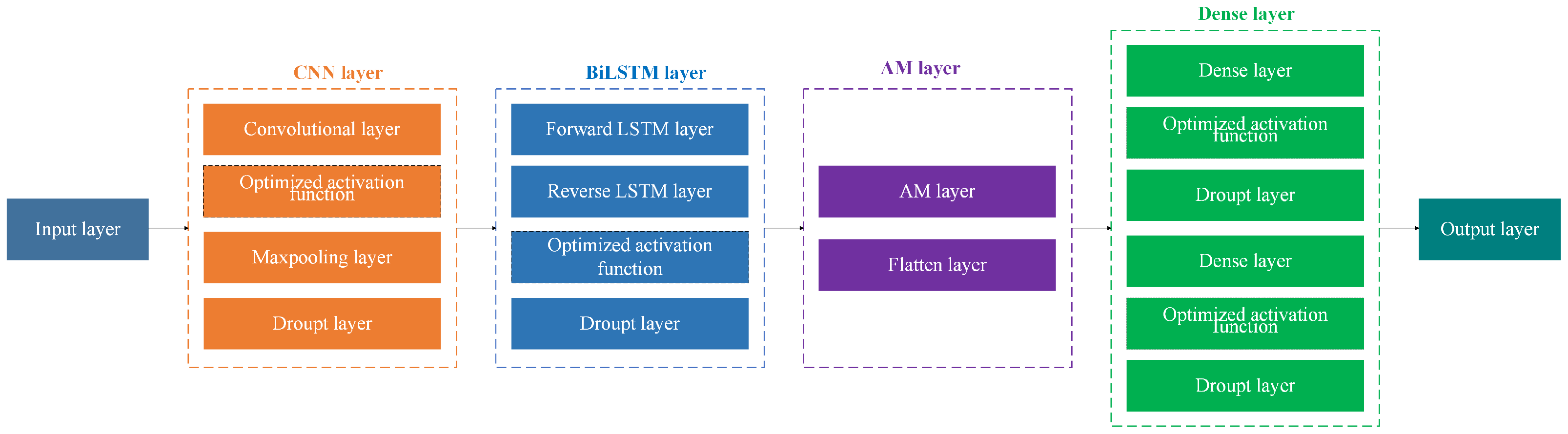

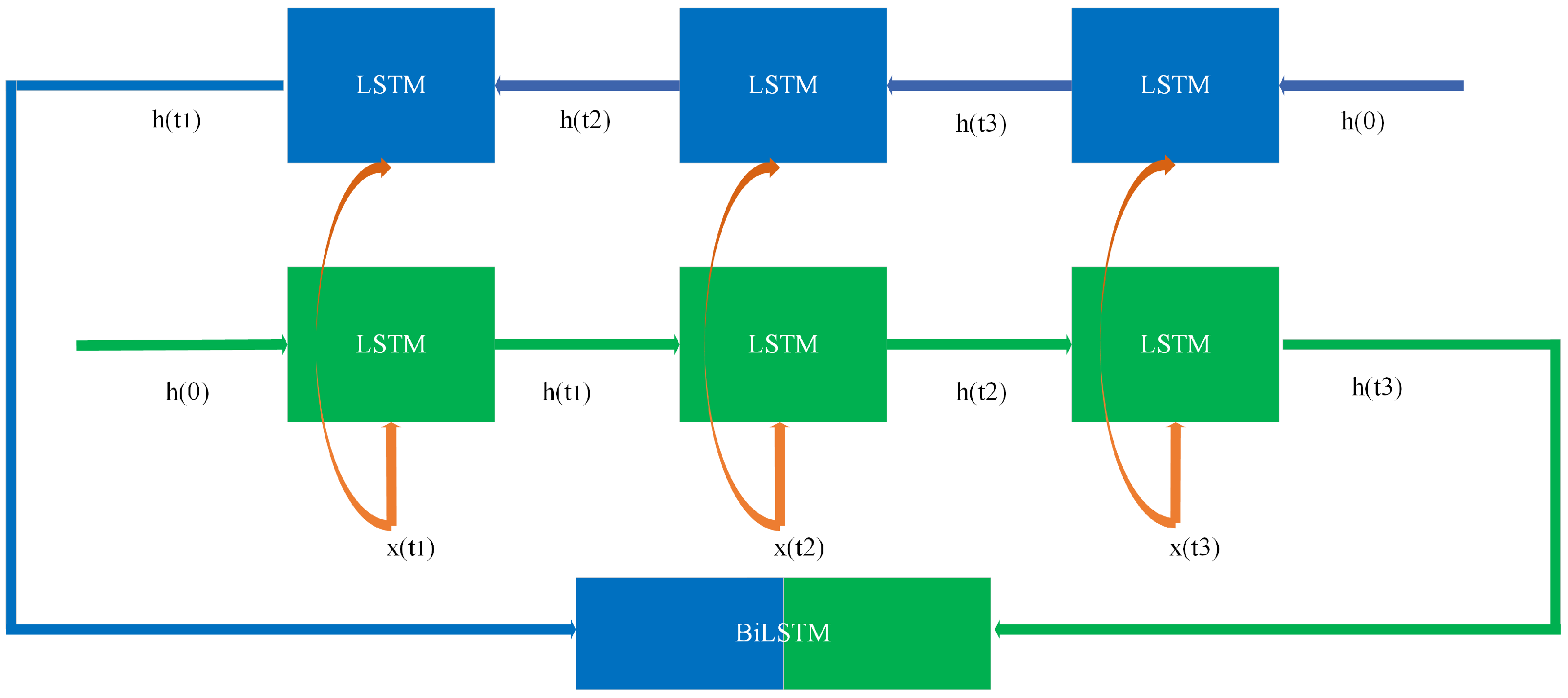
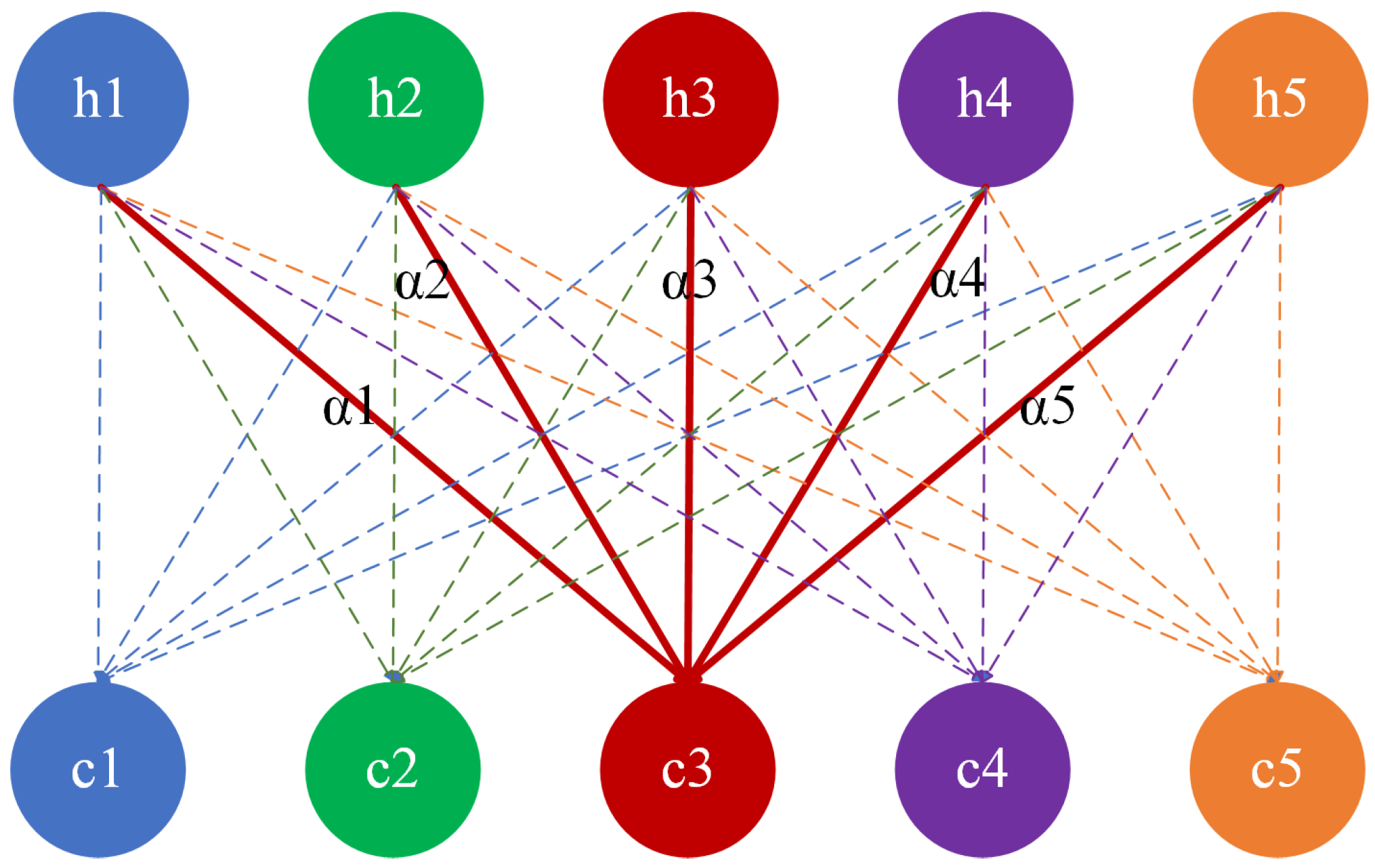
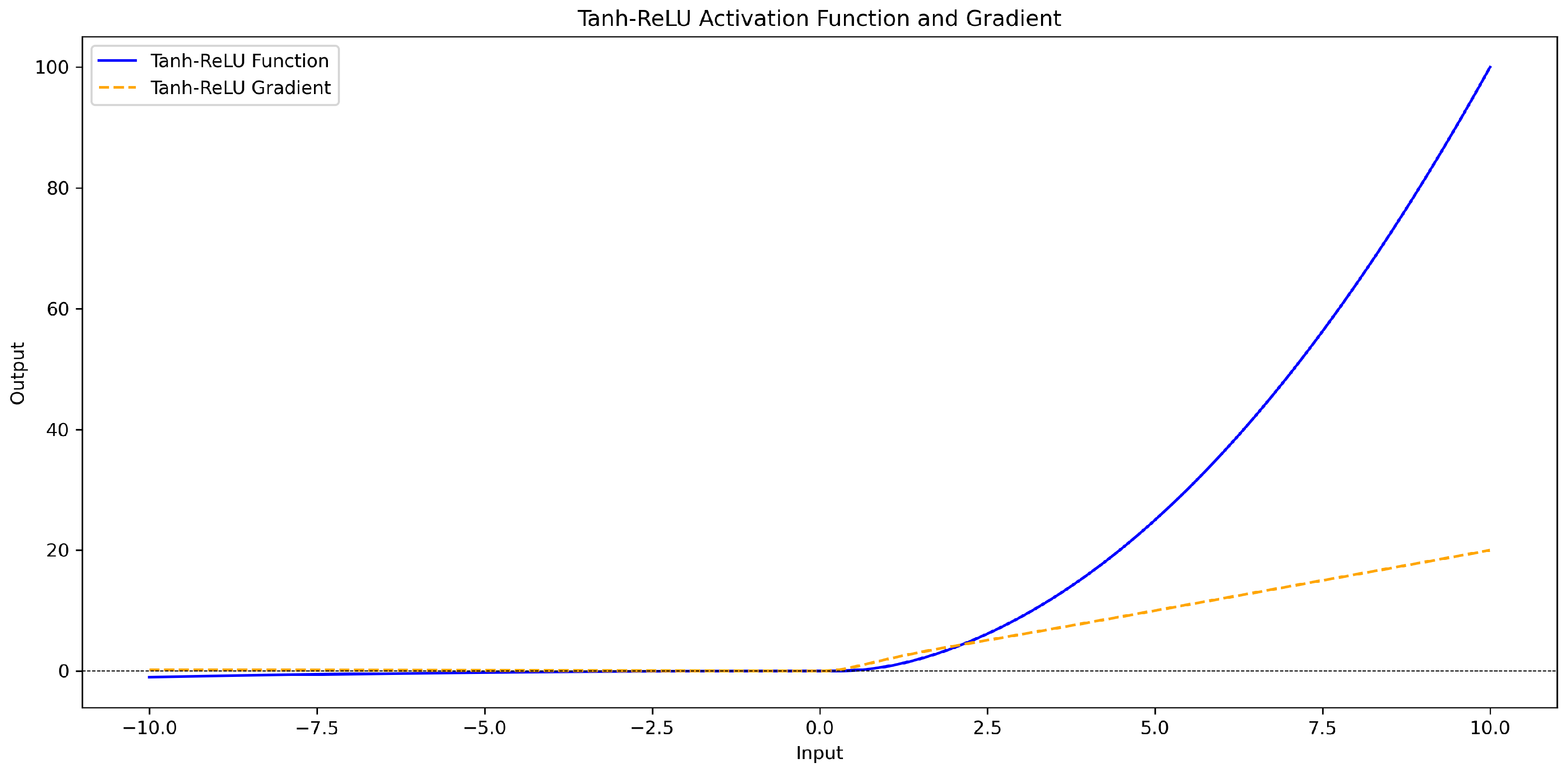
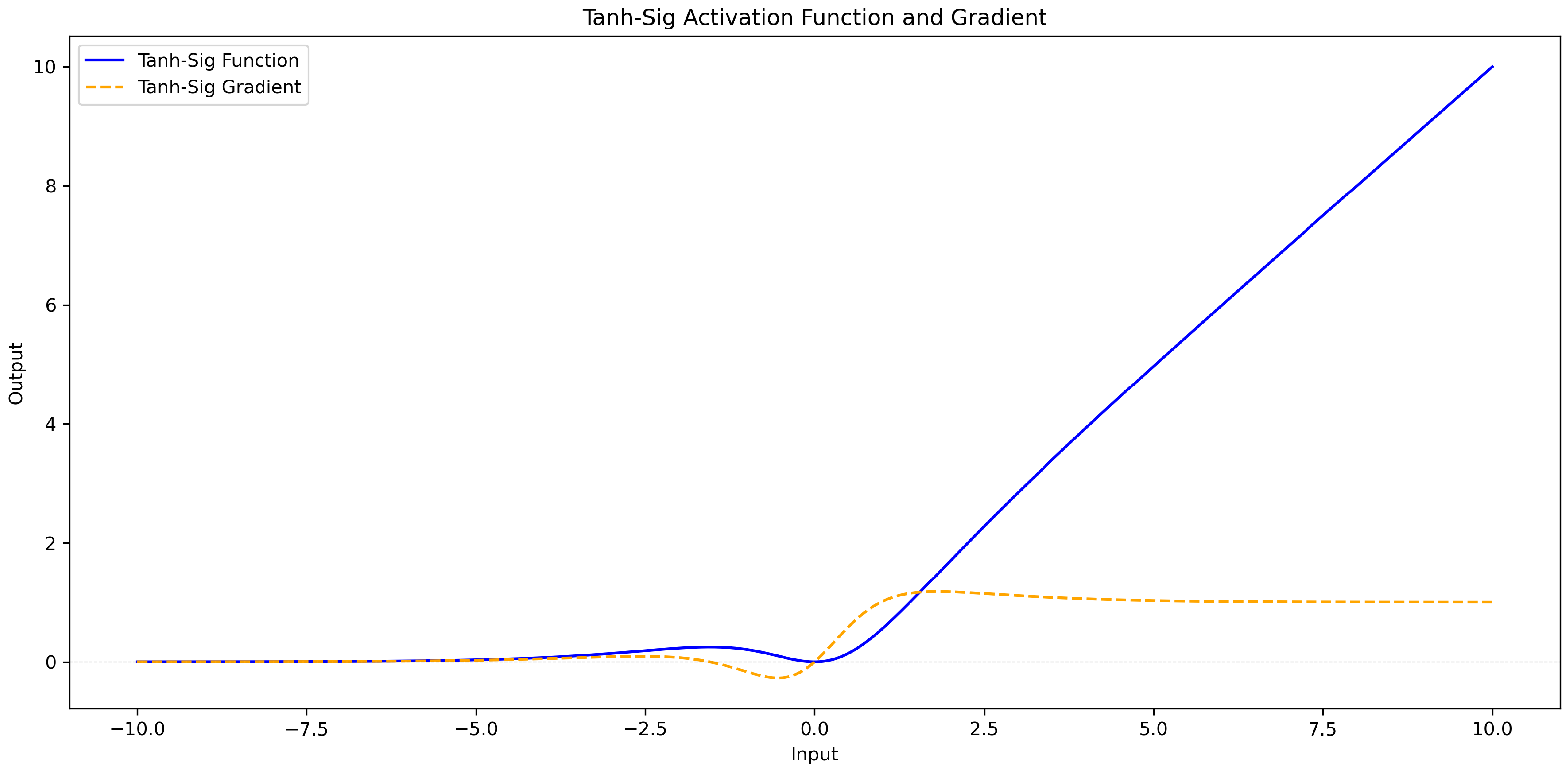
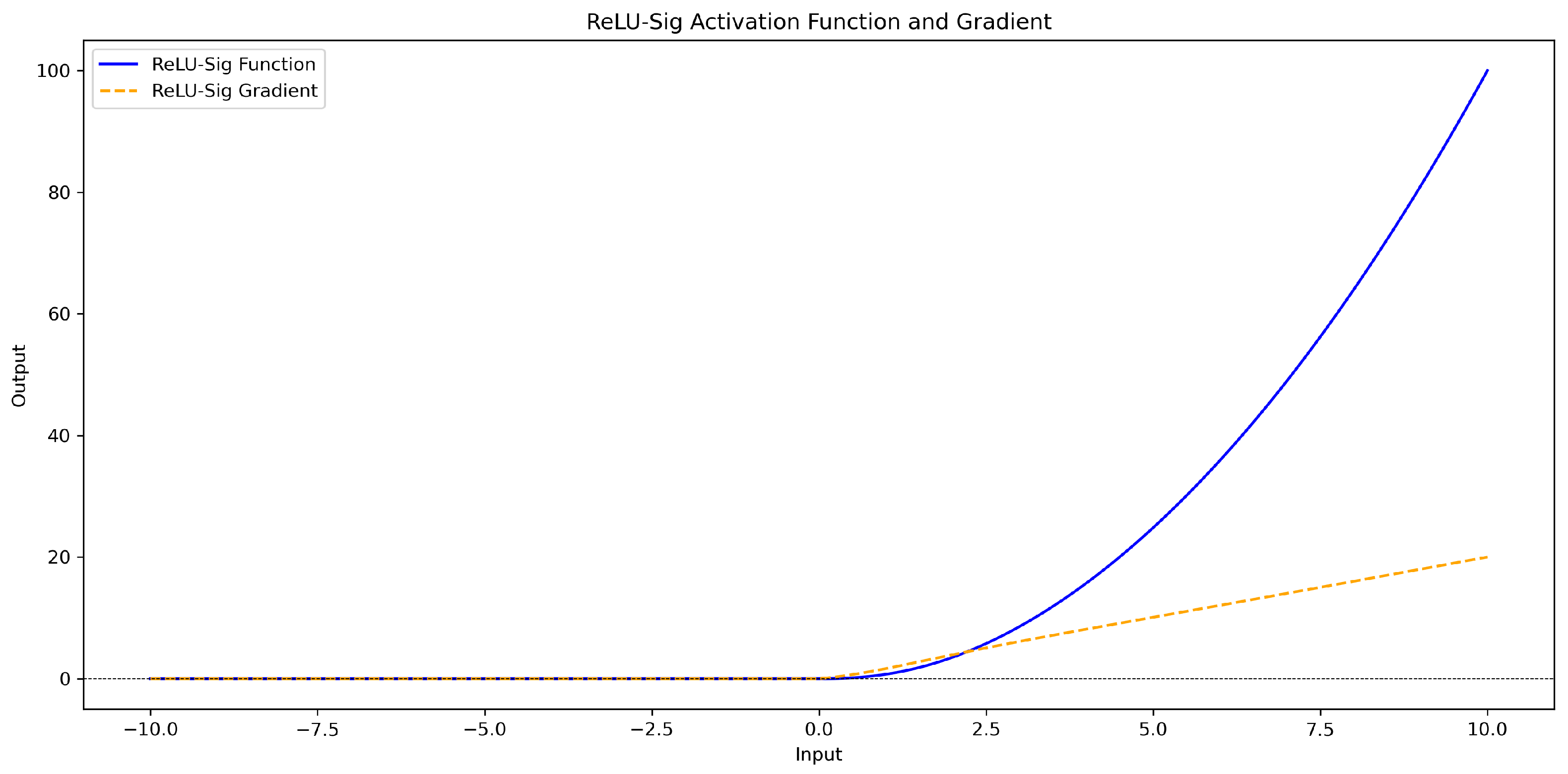


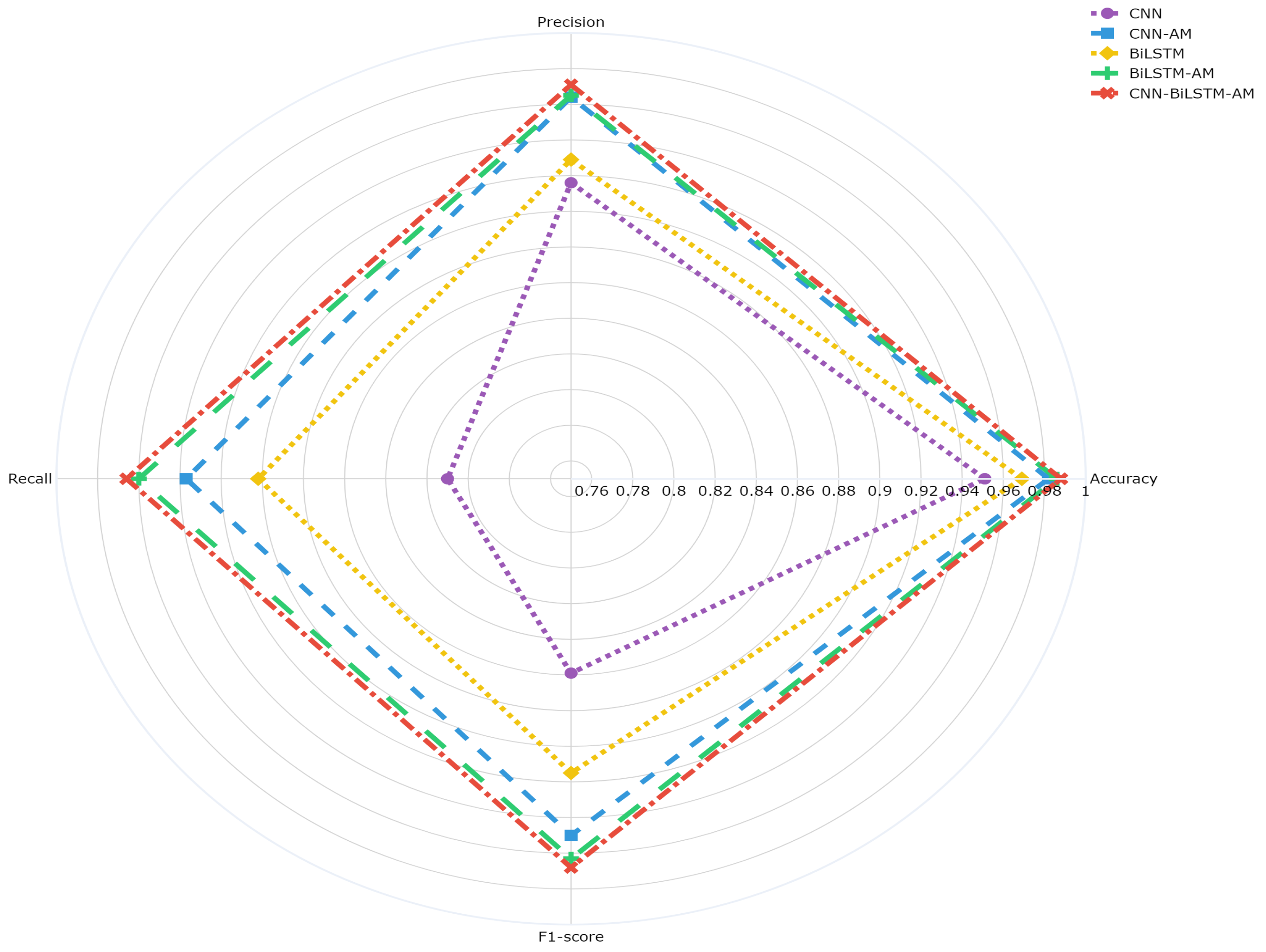
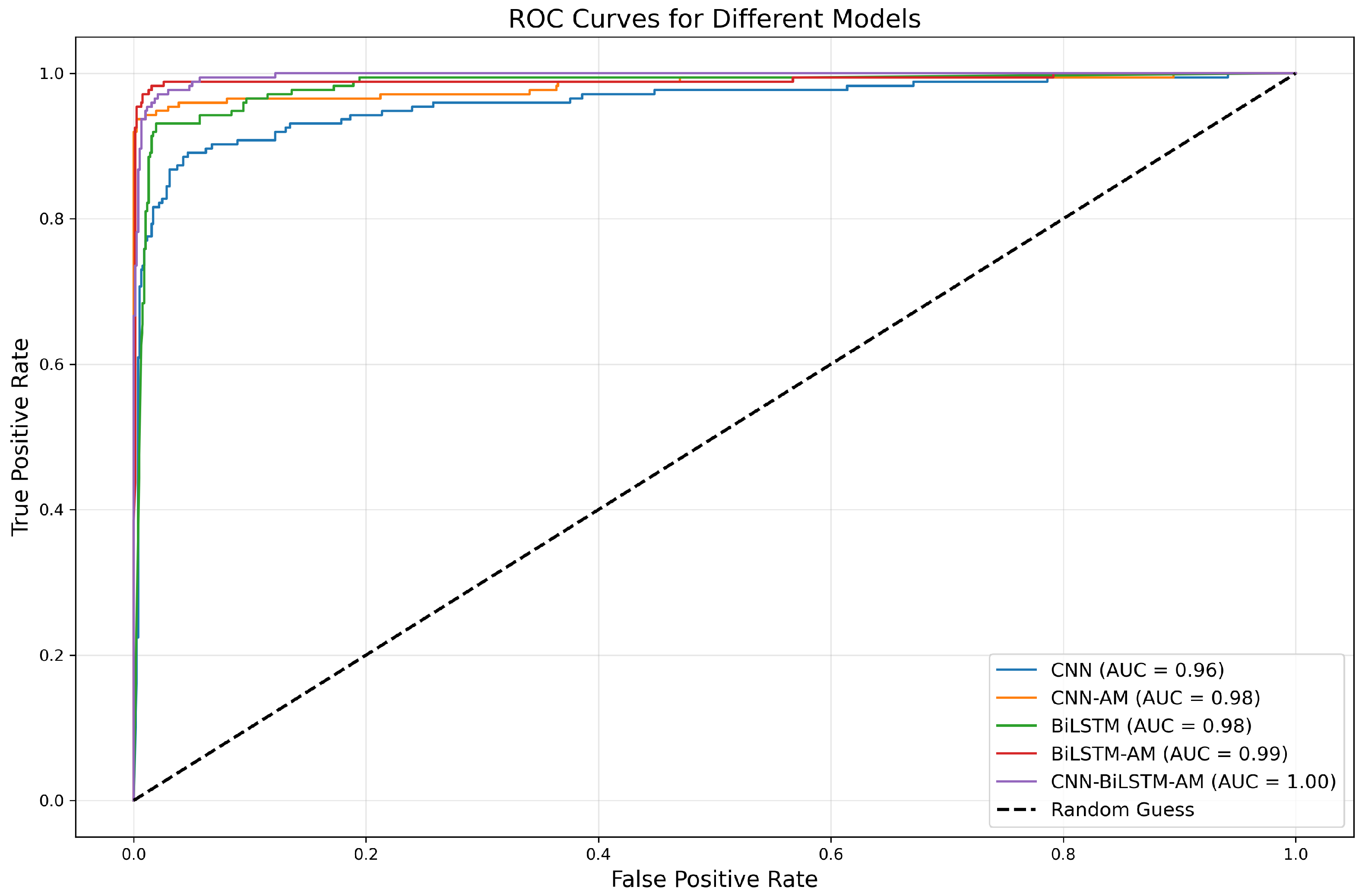
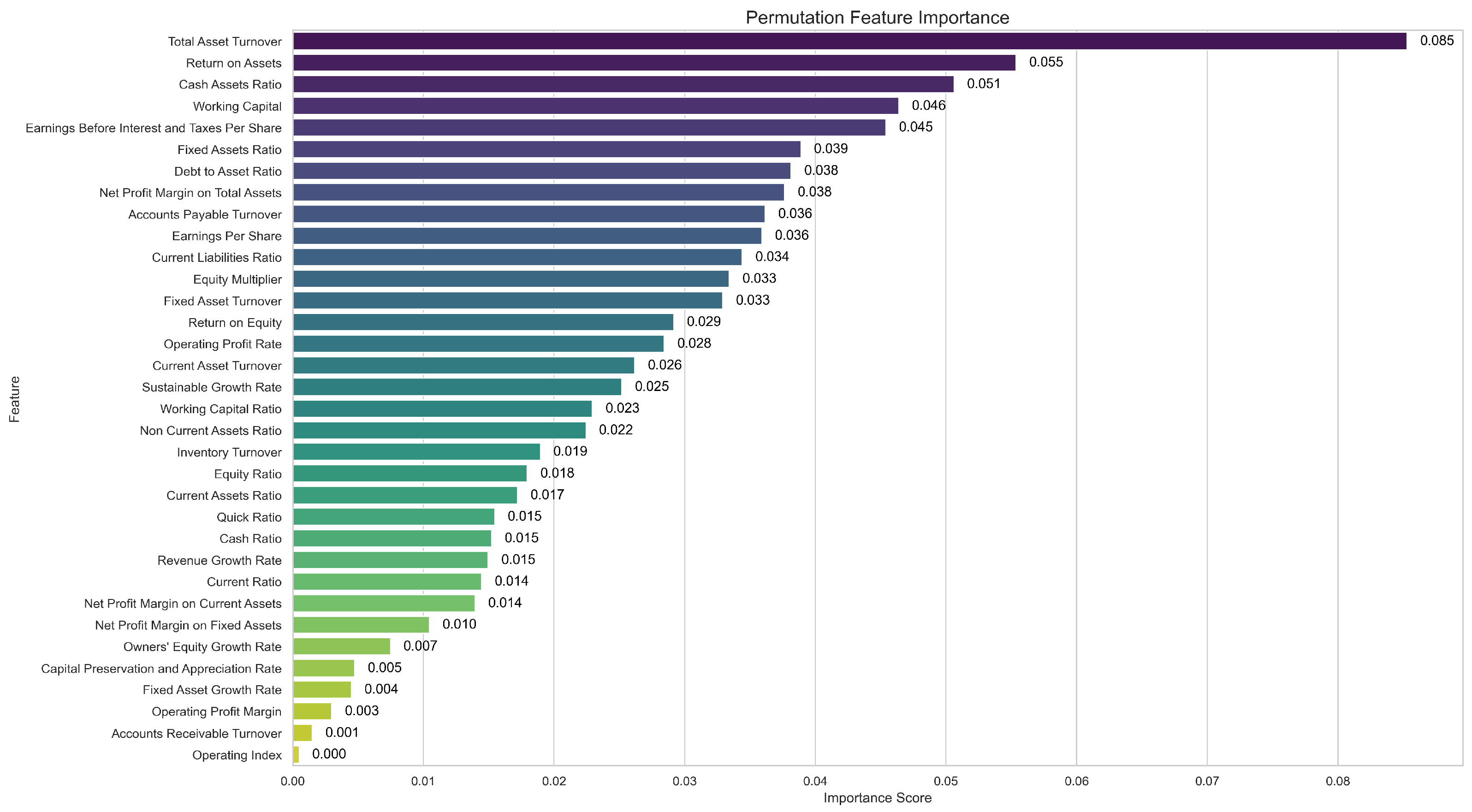
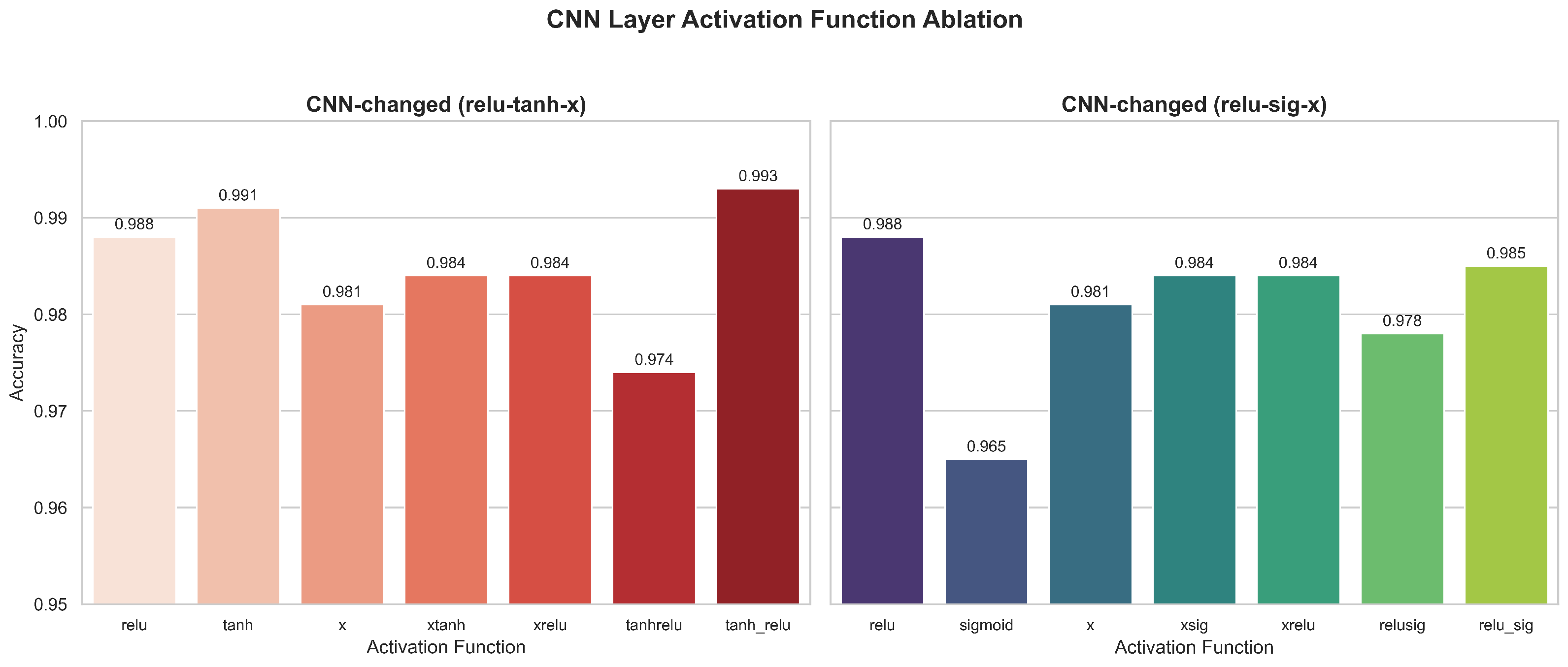
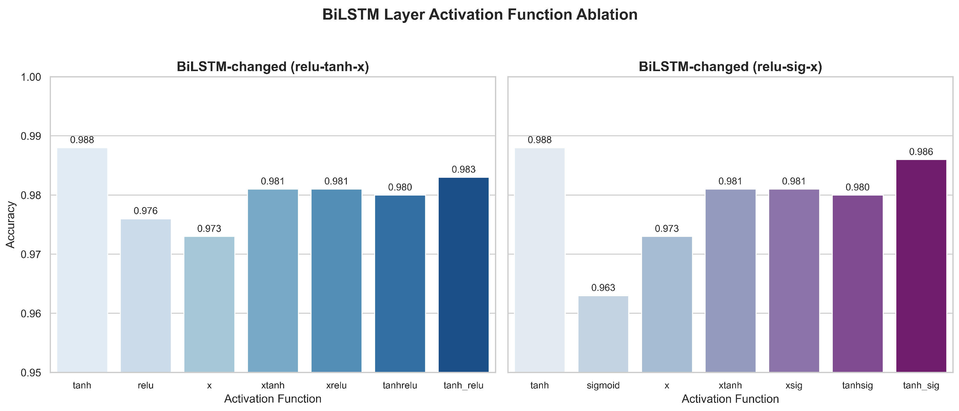
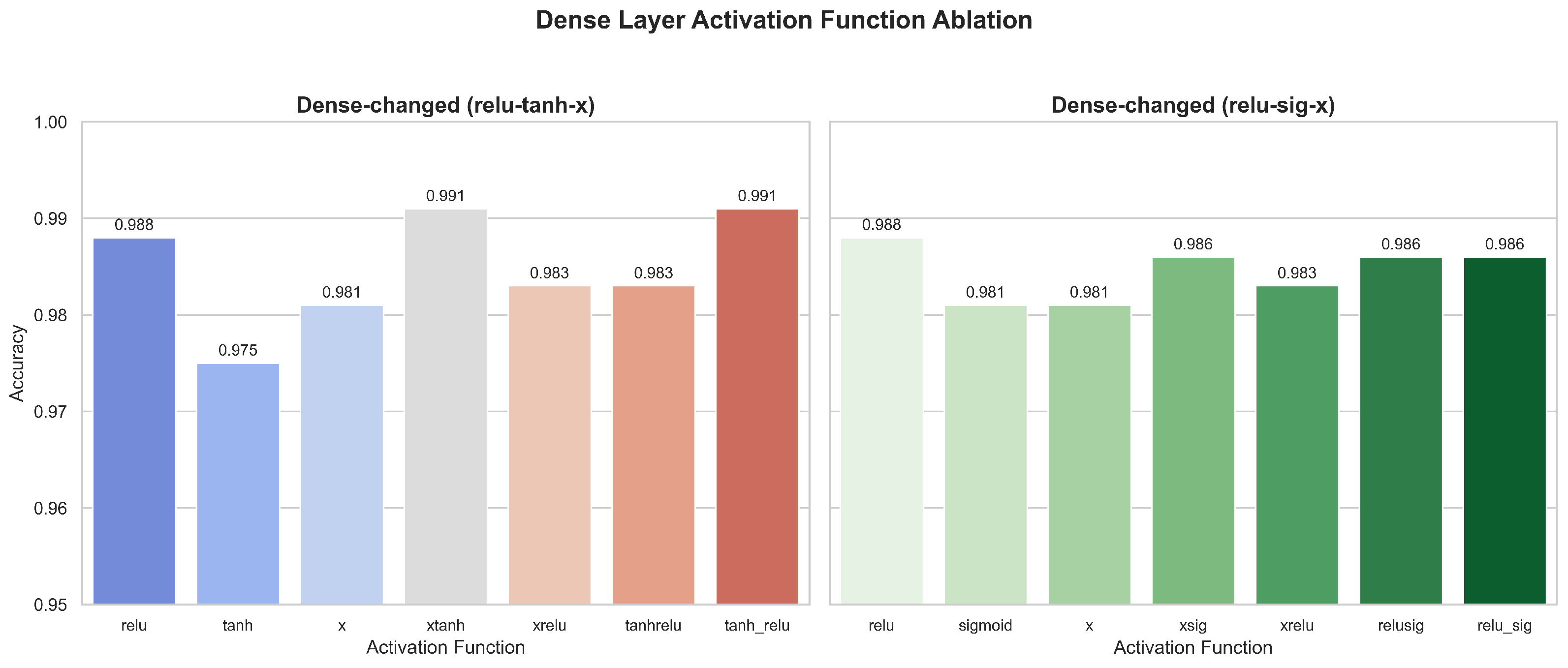
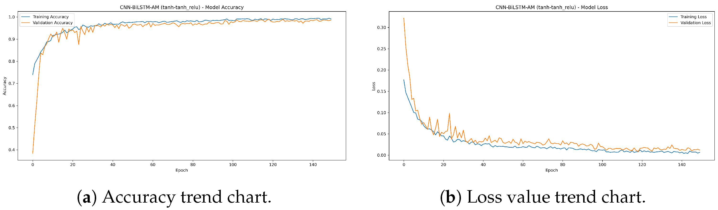

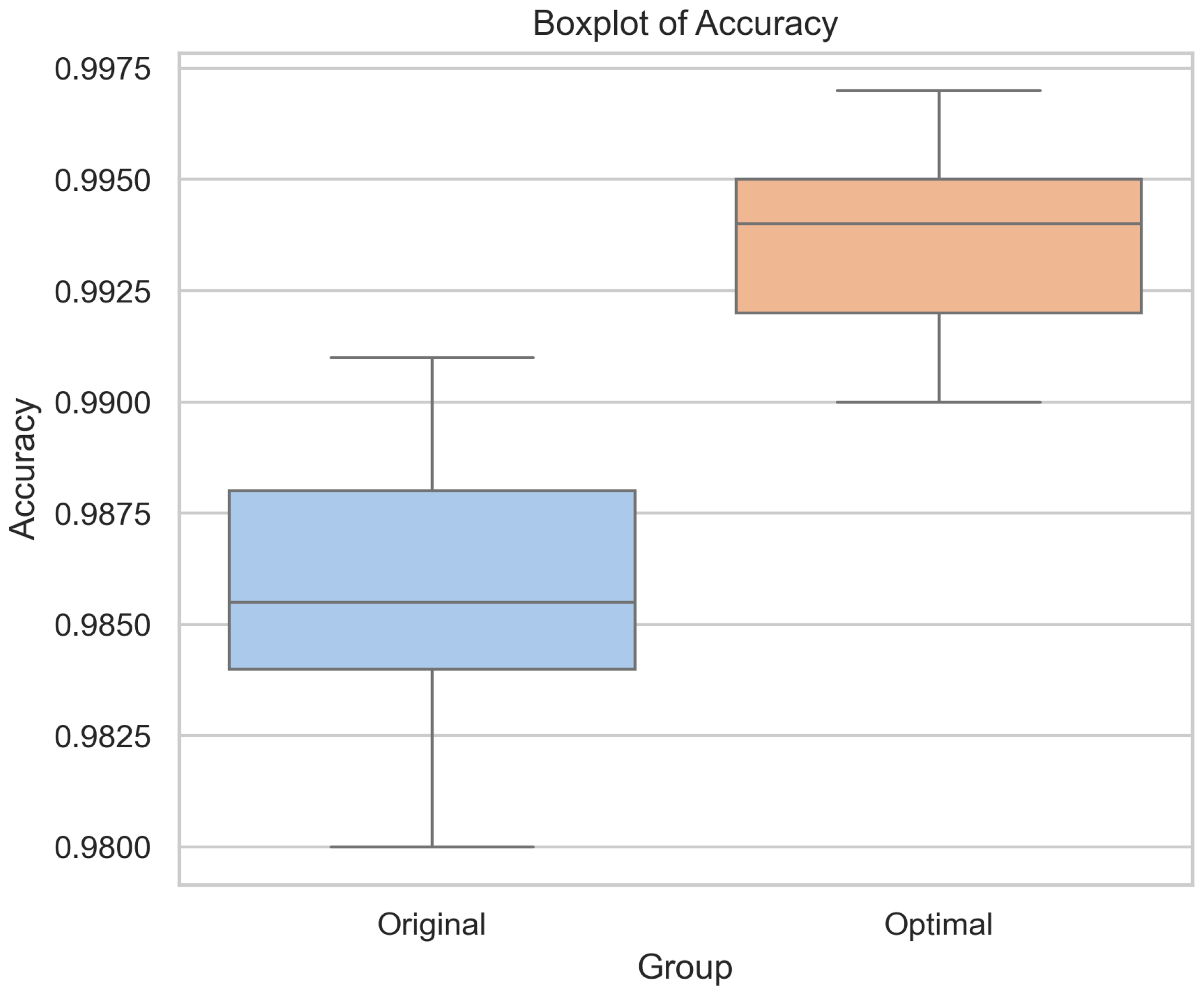
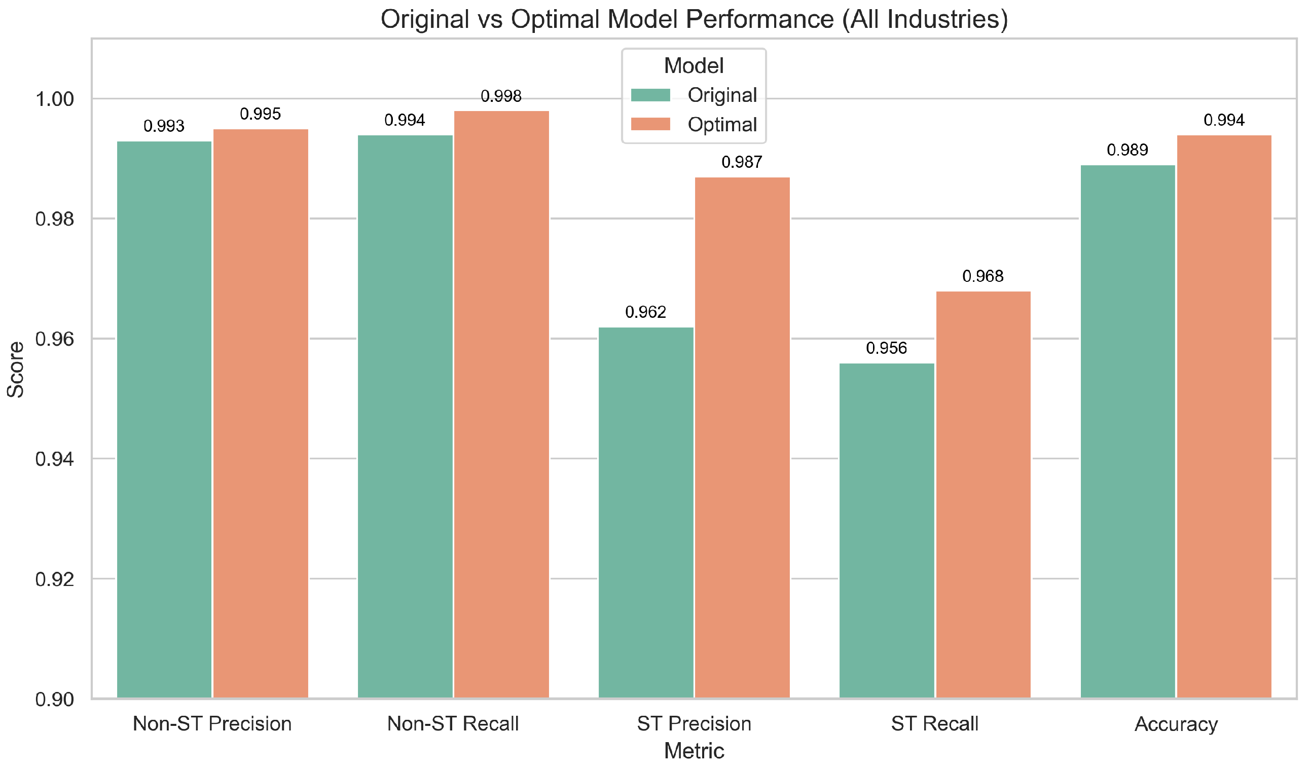
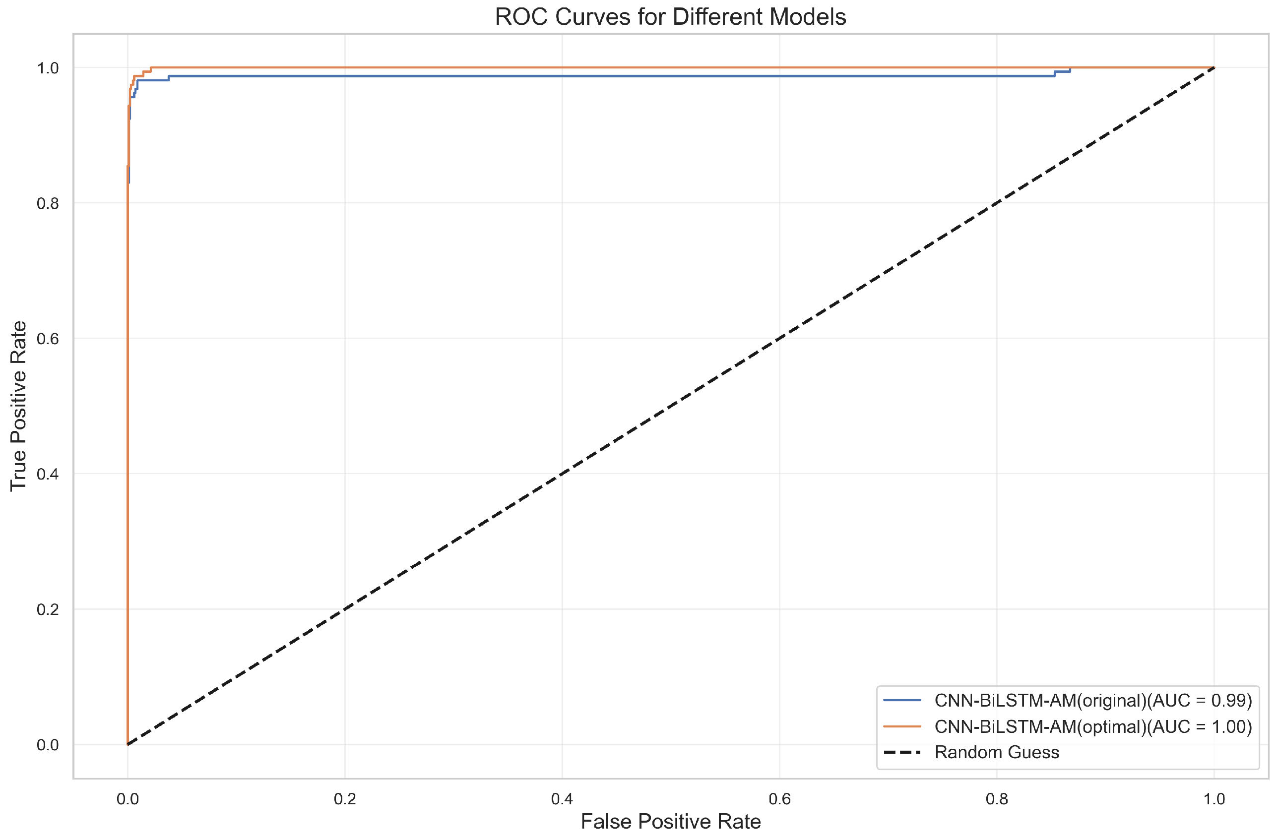
Disclaimer/Publisher’s Note: The statements, opinions and data contained in all publications are solely those of the individual author(s) and contributor(s) and not of MDPI and/or the editor(s). MDPI and/or the editor(s) disclaim responsibility for any injury to people or property resulting from any ideas, methods, instructions or products referred to in the content. |
© 2025 by the authors. Licensee MDPI, Basel, Switzerland. This article is an open access article distributed under the terms and conditions of the Creative Commons Attribution (CC BY) license (https://creativecommons.org/licenses/by/4.0/).