
A Daily Runoff Prediction Model for the Yangtze River Basin Based on an Improved Generative Adversarial Network


Abstract
1. Introduction
- (1)
- This research presents an innovative generative adversarial network framework (VXWGAN-GP) that integrates VAE and WGAN-GP, constructing a daily runoff prediction model that synergistically combines VAE, WGAN-GP, CNN, BiLSTM, GRU, and attention mechanisms.
- (2)
- The encoder of the VAE transforms the input features into a lower-dimensional latent space, whereas the decoder works to restore and merge the data back with the original input data. This process enhances the feature representation and boosts the model’s capacity to grasp complex data structures. Meanwhile, the model employs a CNN-based discriminator to assess the quality of generated data, and the generator integrates the temporal modeling strengths of BiLSTM and GRU, supplemented by an attention mechanism to optimize hydrological feature learning, further improving predictive performance.
- (3)
- The developed framework is implemented for daily streamflow prediction across three key hydrological monitoring sites—Yichang, Cuntan, and Pingshan—located in the upper and middle sections of the Yangtze River basin. Experimental results demonstrate that VXWGAN-GP significantly outperforms LSTM, BiLSTM, GRU, and WGAN-GP in terms of RMSE, MAE, and R2 metrics. Moreover, the model attains the optimal overall performance across representative wet, normal, and dry years, thereby highlighting its reliability and outstanding predictive capabilities.
2. Theoretical Introduction to Prediction Methods
2.1. Improved Generative Adversarial Network (WGAN-GP)
2.2. Bidirectional Long Short-Term Memory Network (BiLSTM)
2.3. Gated Recurrent Unit (GRU)
2.4. Attention Mechanism
2.5. Variational Autoencoder (VAE)
3. Proposed Model (VXWGAN-GP)
3.1. Primary Structure of the Improved WGAN-GP-Based Daily Runoff Prediction Model
- (1)
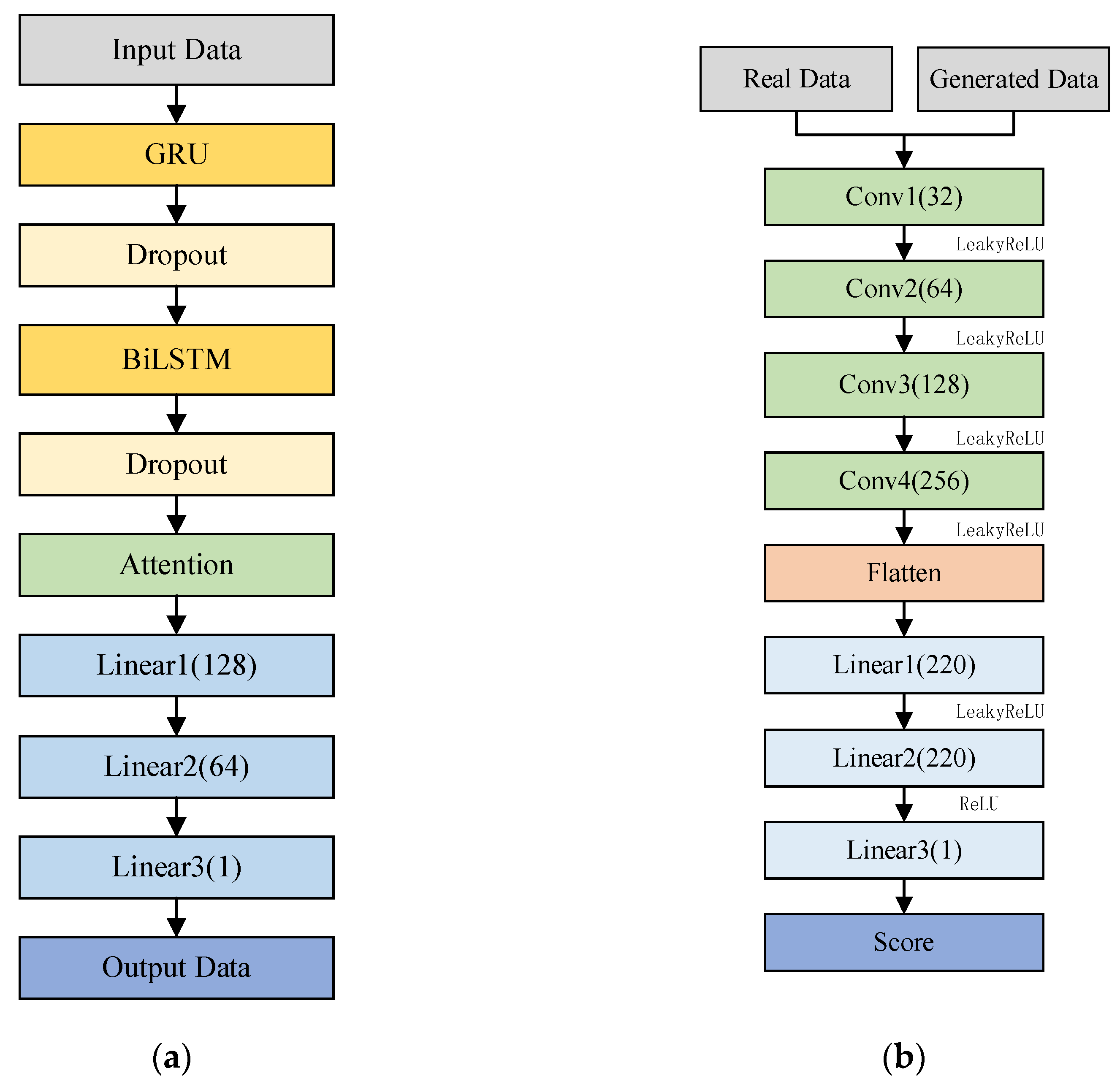
- Generator Structure
- (2)
- Discriminator Structure
3.2. Specific Steps of the Daily Runoff Prediction Model Based on the Improved Generative Adversarial Network
- (1)
- Step 1: Data Loading and Preprocessing. First, daily-scale runoff data and its associated features are acquired, with missing values and outliers removed to ensure data completeness and accuracy. All data are normalized to the range [0, 1] to eliminate the influence of different scales on the model. Subsequently, the dataset is divided into a calibration period (80% of the total data) and a validation period (20% of the total data).
- (2)
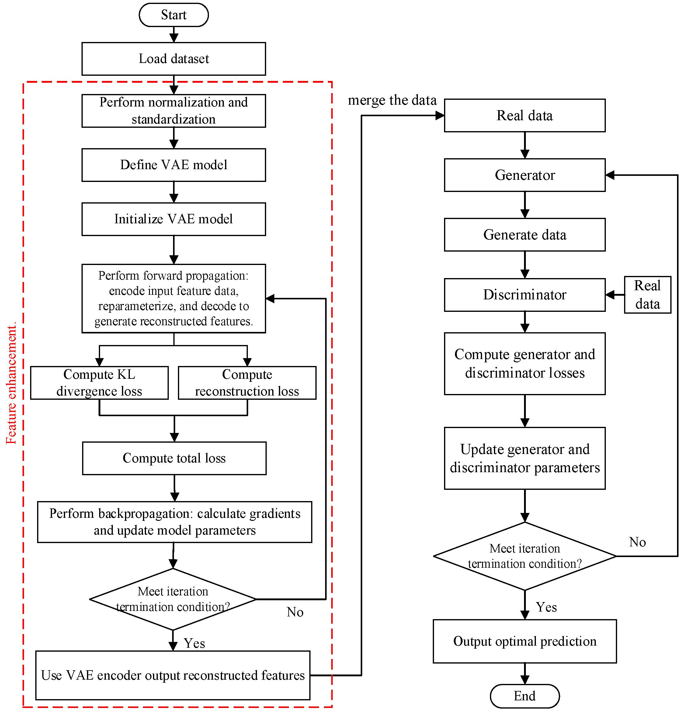
- Step 2: Feature Enhancement Using Variational Autoencoder (VAE). In this step, a VAE is employed for feature enhancement. The encoder part of the VAE maps the input to a multi-dimensional latent space through a multi-layer fully connected network, with each dimension representing a latent variable. The decoder part maps the representations from the latent space back to the input space. The model utilizes the reparameterization trick to approximate a Gaussian distribution, enabling sampling from the latent space. The training objective is to minimize the sum of the reconstruction loss and the KL divergence loss, where the KL divergence term ensures that the distribution of the latent space approximates a standard normal distribution. In each training epoch, the reconstruction loss and KL divergence are computed, and the model parameters are updated through backpropagation. The trained VAE model is then used to enhance the features, generating reconstructed features that are combined with the original features and fed into the forecasting model.
- (3)
- Step 3: Transforming Time-Series Data Using a Sliding Window Method. A sliding window method is adopted to transform the time-series data into a format suitable for model training. The sliding window size is set to 3, where each input sample includes data from the previous three time steps, and the output corresponds to the target value of the fourth time step.
- (4)
- Step 4: Constructing the Generator and Discriminator with Adversarial Training. The generator, which integrates GRU, BiLSTM, and an attention mechanism, learns the distribution characteristics of the time-series data and generates predictions for future time steps. The discriminator evaluates the discrepancy between the generated data and the real data through adversarial training, thereby optimizing the generator’s predictive capability. The generator and discriminator are trained alternately, continuously improving prediction accuracy.
- (5)
- Step 5: Model Prediction and Performance Evaluation. Finally, the trained generator is used to make predictions, and the predicted results are compared with the actual data. By evaluating various performance metrics, the effectiveness and accuracy of the model are validated.
4. Model Evaluation Metrics
5. Case Study
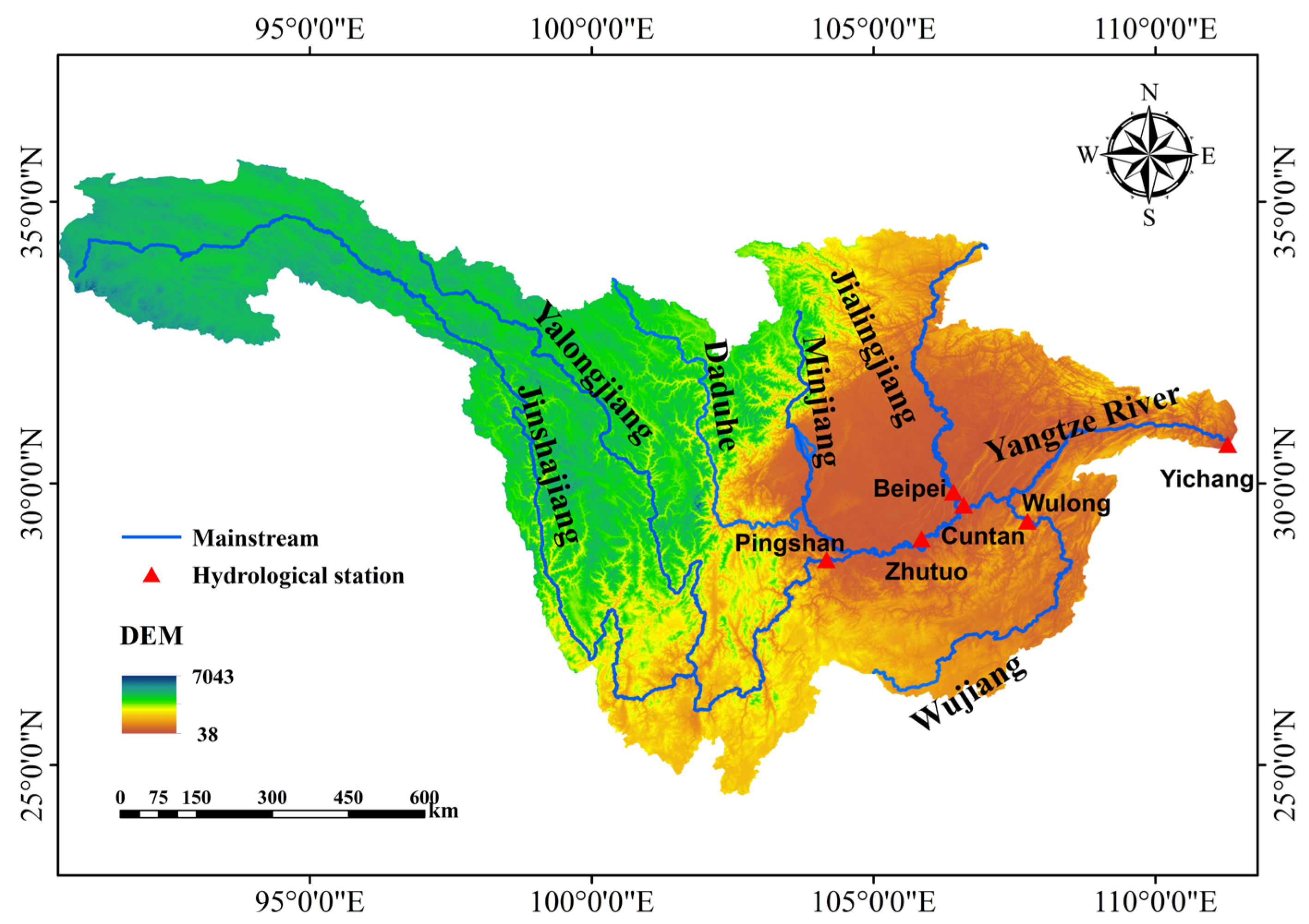
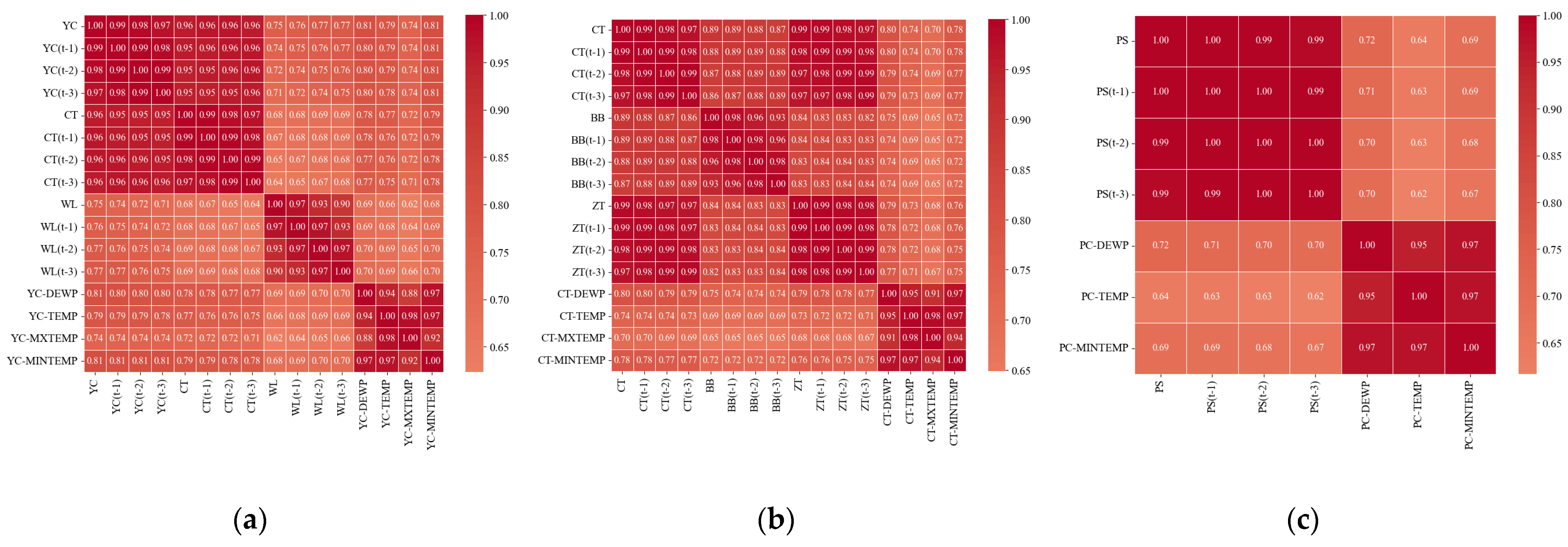
5.1. Study Area and Feature Selection
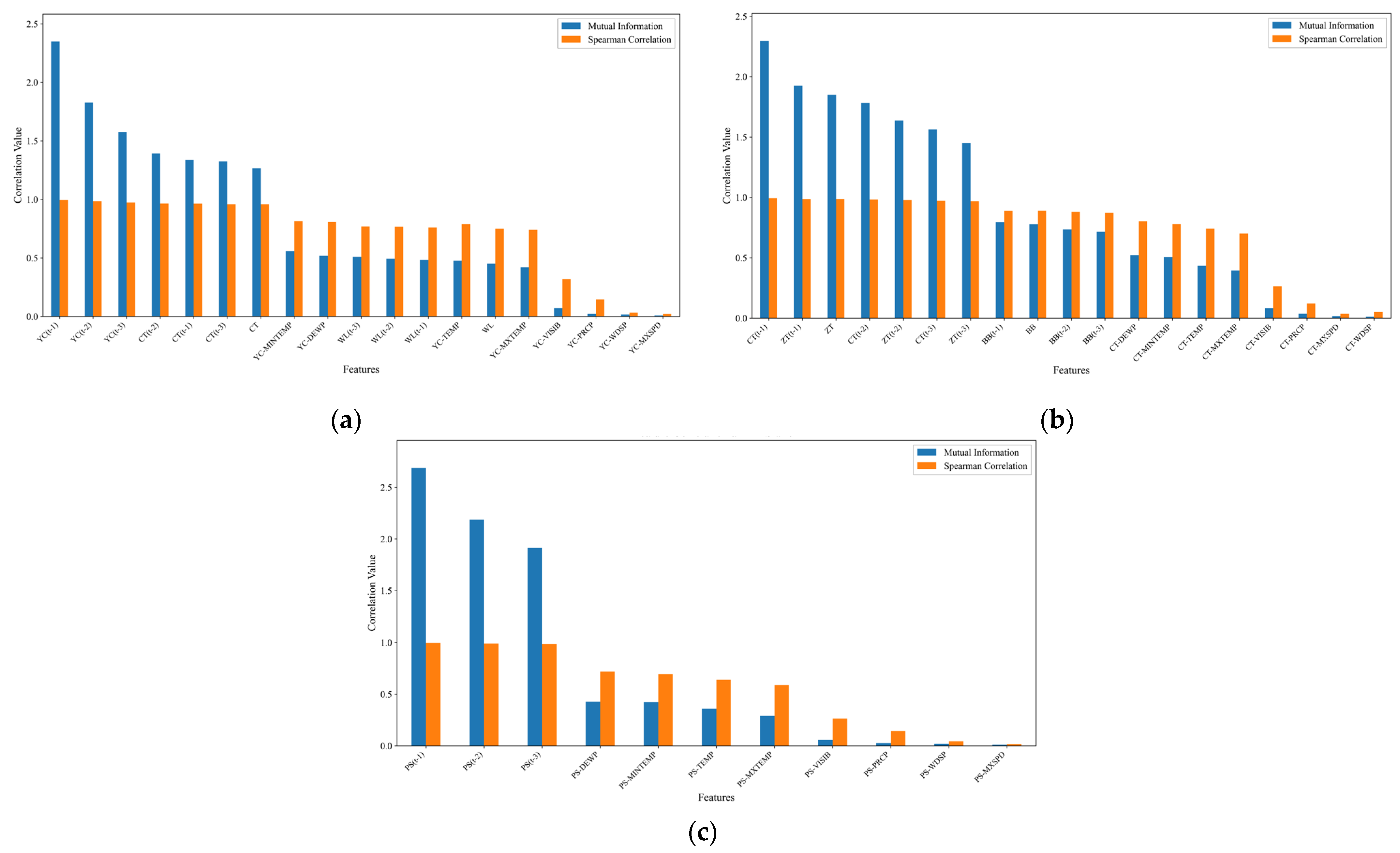
- Runoff-related factors: Measured runoff at Yichang Station for the previous 1, 2, and 3 days (YC(t − 1), YC(t − 2), YC(t − 3)); real-time and previous 1-, 2-, and 3-day runoff at Cuntan Station (CT, CT(t − 1), CT(t − 2), CT(t − 3)); and real-time and previous 1-, 2-, and 3-day runoff at Wulong Station (WL, WL(t − 1), WL(t − 2), WL(t − 3)).
- Meteorological factors: Dew point temperature (YC-DEWP), maximum temperature (YC-MXTEMP), minimum temperature (YC-MINTEMP), and average temperature (YC-TEMP) at Yichang Station.
- Runoff-related factors: Measured runoff at Cuntan Station for the previous 1, 2, and 3 days (CT(t − 1), CT(t − 2), CT(t − 3)); real-time and previous 1-, 2-, and 3-day runoff at Beibei Station (BB, BB(t − 1), BB(t − 2), BB(t − 3)); and real-time and previous 1-, 2-, and 3-day runoff at Zhutuo Station (ZT, ZT(t − 1), ZT(t − 2), ZT(t − 3)).
- Meteorological factors: Dew point temperature (CT-DEWP), maximum temperature (CT-MXTEMP), minimum temperature (CT-MINTEMP), and average temperature (CT-TEMP) at Cuntan Station.
- Runoff-related factors: Measured runoff at Pingshan Station for the previous 1, 2, and 3 days (PS(t − 1), PS(t − 2), PS(t − 3)).
- Meteorological factors: Dew point temperature (PS-DEWP), minimum temperature (PS-MINTEMP), and average temperature (PS-TEMP) at Pingshan Station.
5.2. Comparative Experiments and Parameter Settings
6. Results Analysis and Discussion
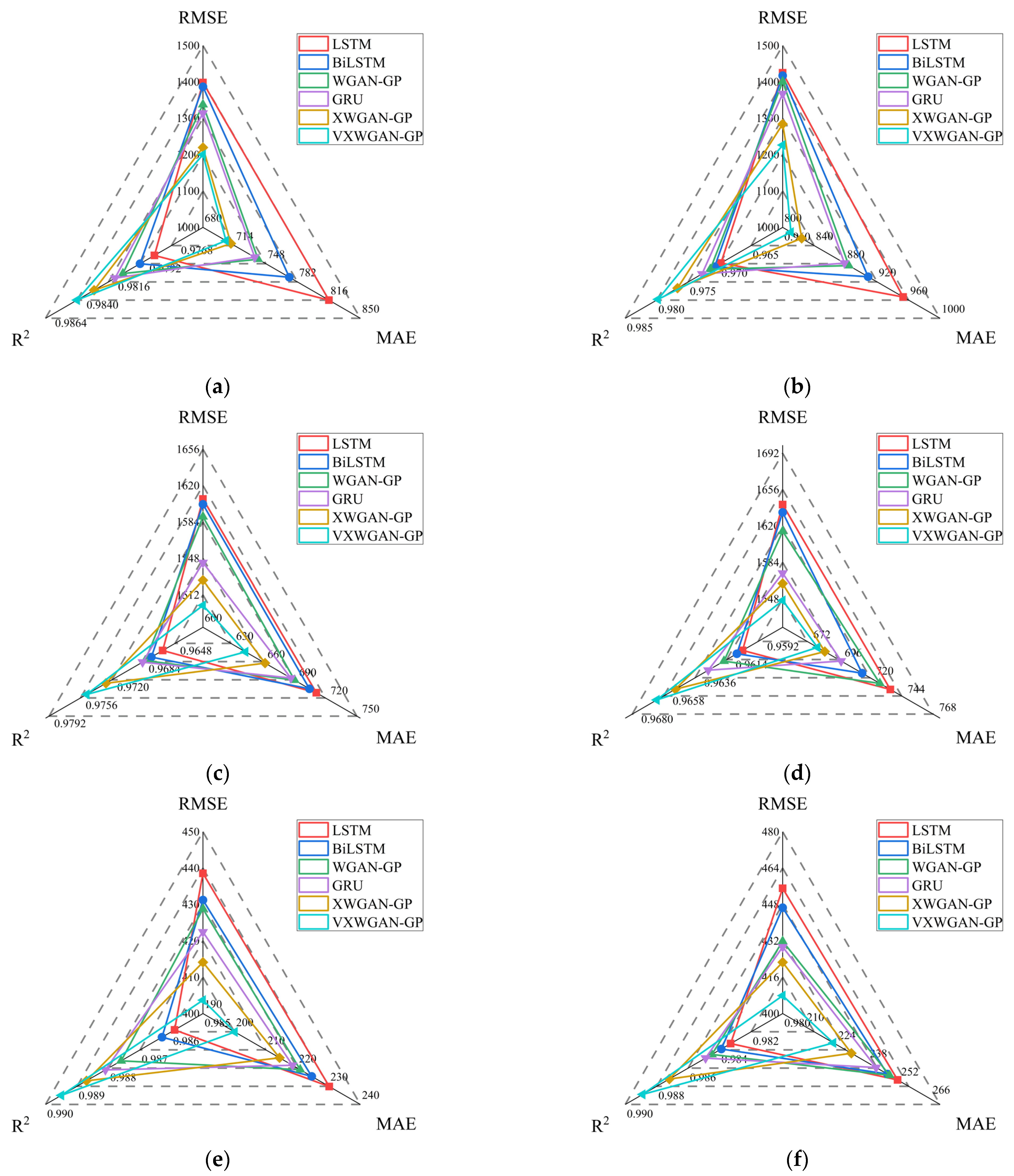
6.1. Analysis of Model Evaluation Metrics Calculation Results
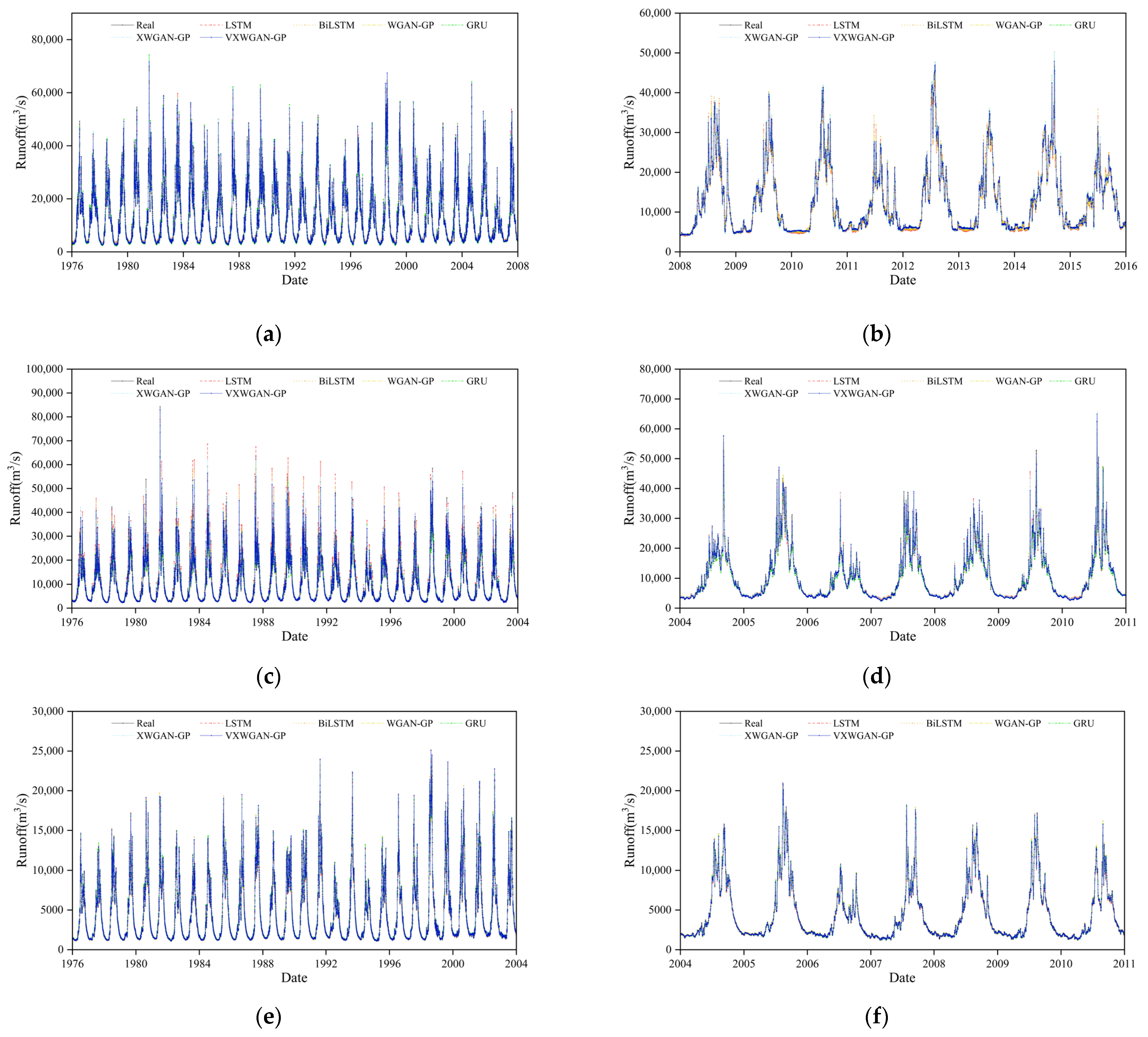
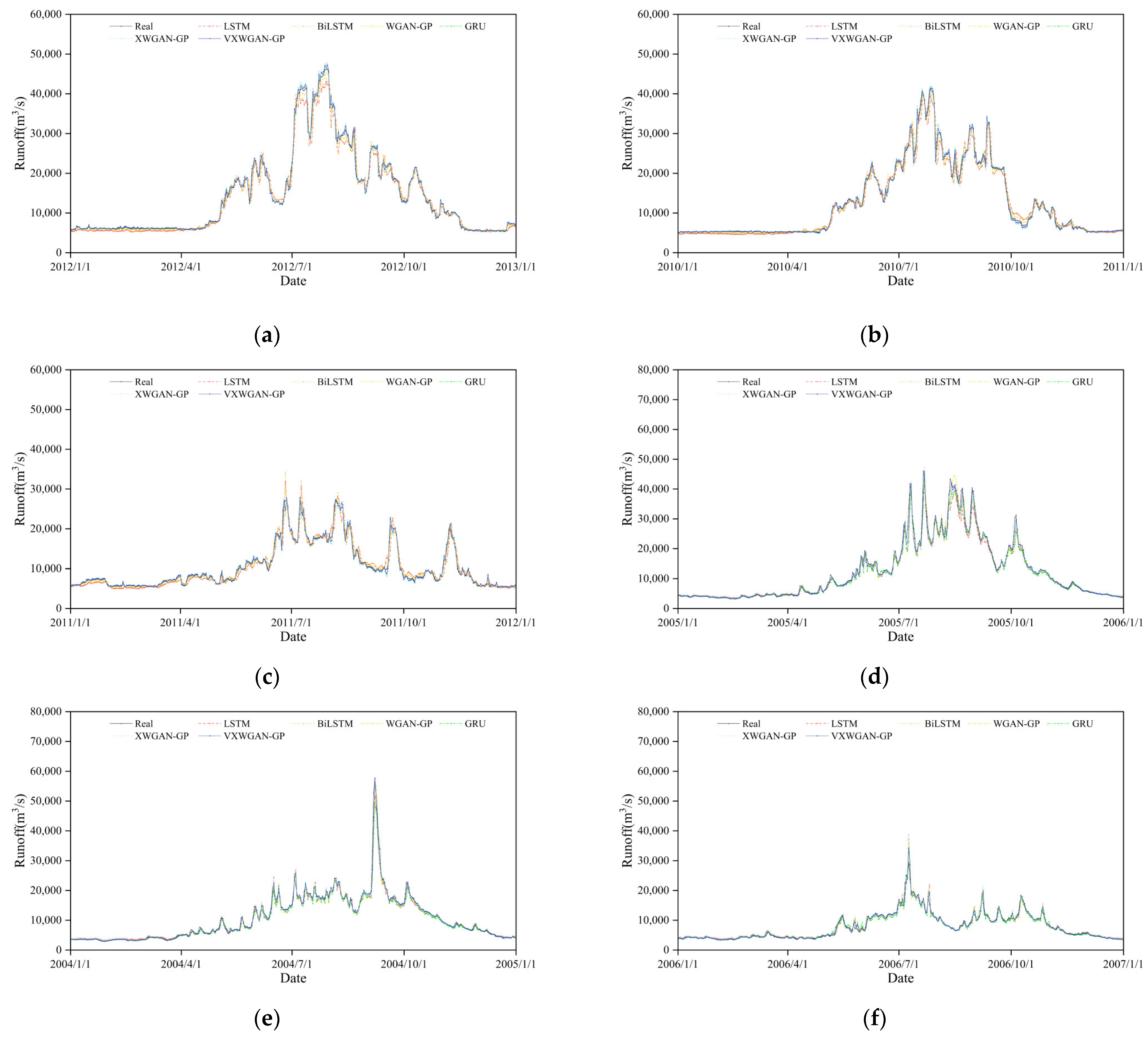
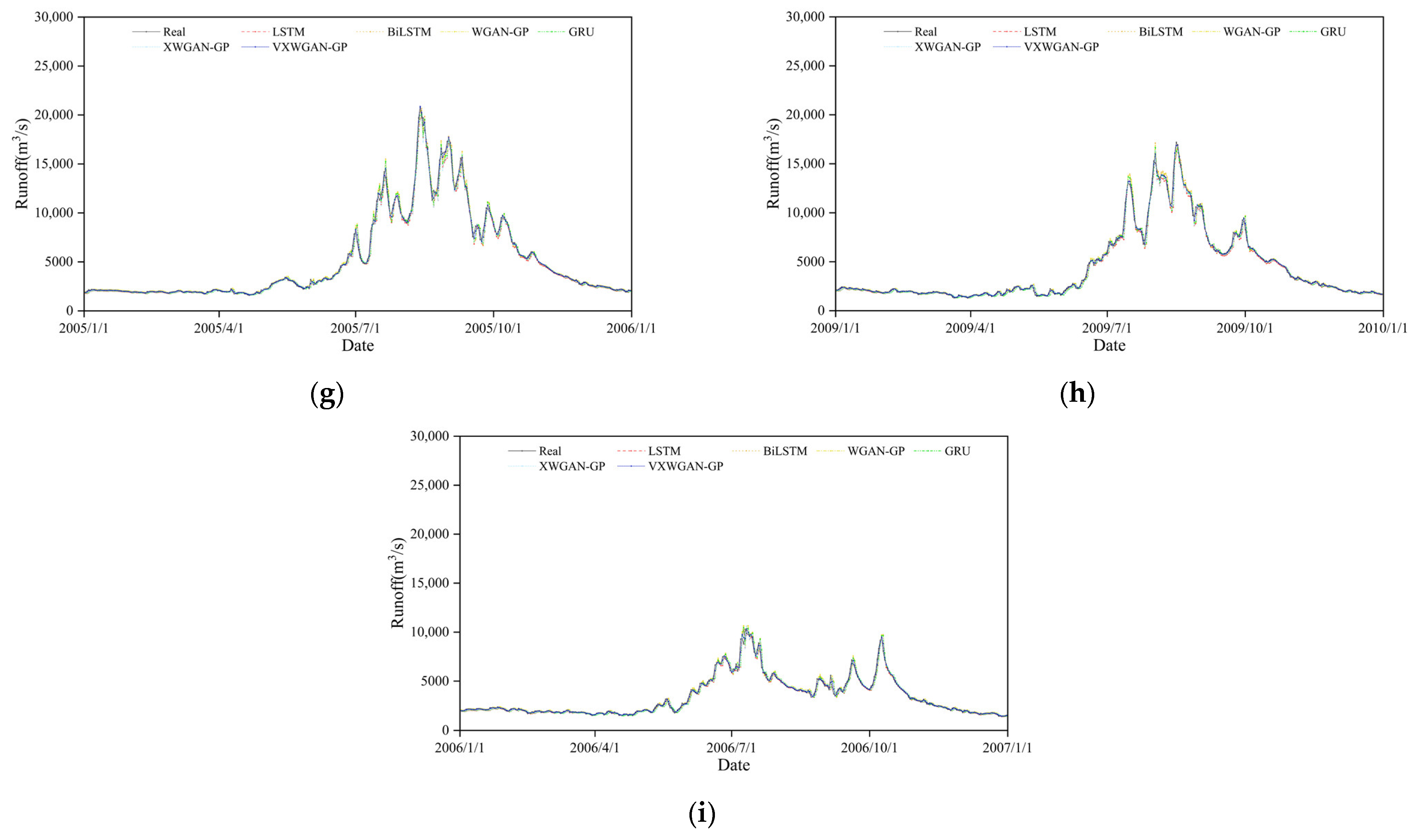
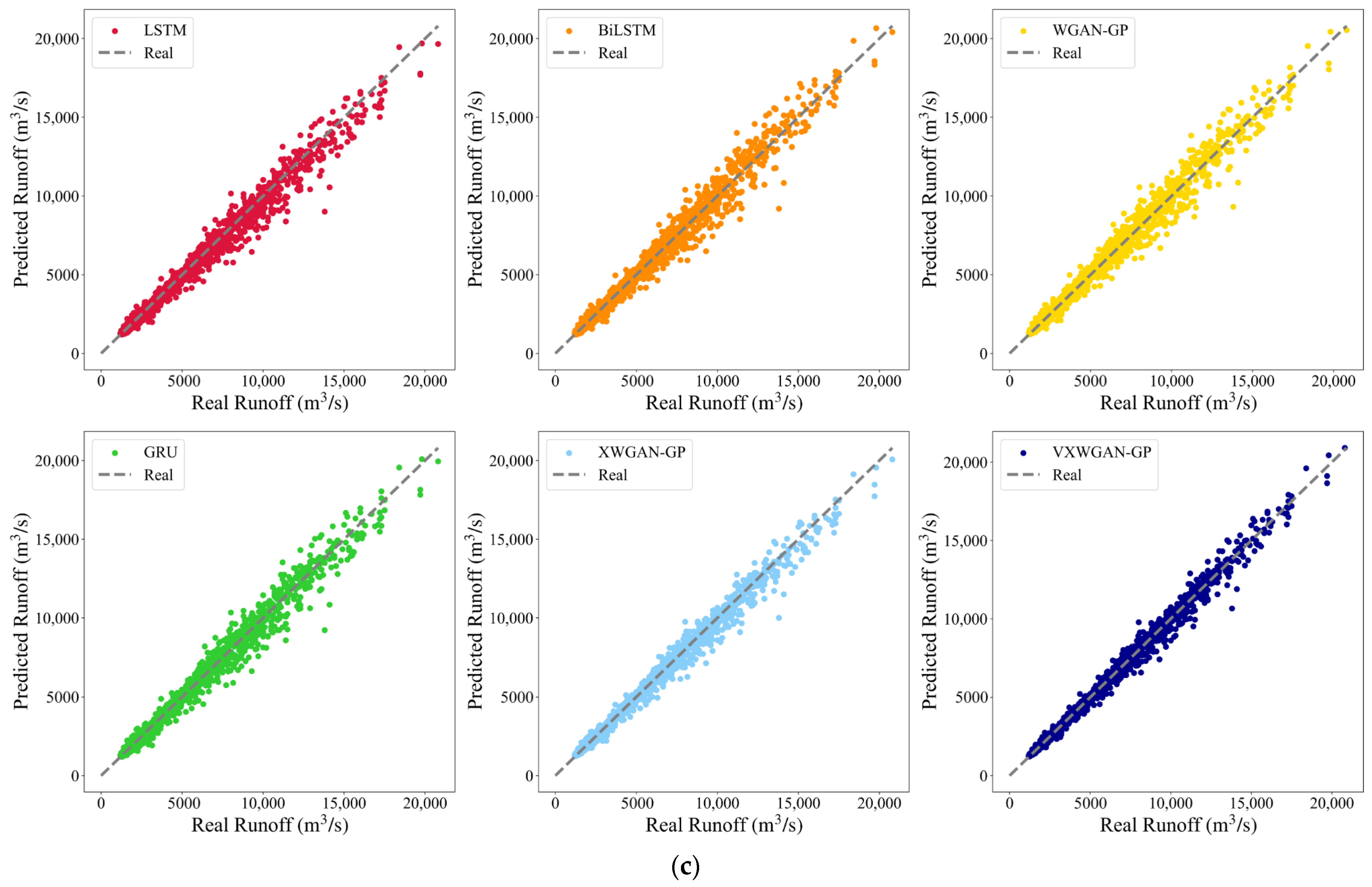
6.2. Analysis of Model Reliability and Applicability
7. Conclusions
- (1)
- Superior predictive performance: Through comparative analysis with benchmark models, the VXWGAN-GP model demonstrated superior performance across all evaluation metrics at the Yichang, Cuntan, and Pingshan stations. Its scatter plots exhibited a better overall trend fit than other models. Under three distinct hydrological conditions, the predicted runoff curves closely aligned with observed values, further confirming that the proposed model, based on an improved generative adversarial network, effectively enhances the accuracy and stability of hydrological runoff forecasting.
- (2)
- Effectiveness of VAE-based feature enhancement: This study validates the effectiveness and reliability of the VXWGAN-GP model, which integrates VAE for feature enhancement in daily-scale runoff forecasting. Experimental results indicate that, compared to XWGAN-GP, the proposed model achieves an R2 improvement of 0.0031 at the Yichang station, with MAE and RMSE reductions of 13.556 and 57.556, respectively. At the Cuntan station, R2 increases by 0.0013, with MAE and RMSE reductions of 5.556 and 16.556, respectively. Similarly, at the Pingshan station, R2 improves by 0.0017, while MAE and RMSE decrease by 8.000 and 14.676, respectively.
- (3)
- Future research directions: Although the VXWGAN-GP model demonstrates strong accuracy and generalization ability in runoff forecasting, its complex architecture increases the computational cost. Future research could explore lightweight deep learning models or leverage techniques such as knowledge distillation to reduce the model complexity. By optimizing the model structure while maintaining predictive accuracy, computational efficiency can be further improved.
Author Contributions
Funding
Institutional Review Board Statement
Informed Consent Statement
Data Availability Statement
Conflicts of Interest
References
- Zhang, J.; Chen, X.; Khan, A.; Zhang, Y.-K.; Kuang, X.; Liang, X.; Taccari, M.L.; Nuttall, J. Daily runoff forecasting by deep recursive neural network. J. Hydrol. 2021, 596, 126067. [Google Scholar]
- Zhu, S.; Wei, J.; Zhang, H.; Xu, Y.; Qin, H. Spatiotemporal deep learning rainfall-runoff forecasting combined with remote sensing precipitation products in large scale basins. J. Hydrol. 2023, 616, 128727. [Google Scholar]
- Li, H.; Zhang, C.; Chu, W.; Shen, D.; Li, R. A process-driven deep learning hydrological model for daily rainfall-runoff simulation. J. Hydrol. 2024, 637, 131434. [Google Scholar]
- Li, T.; Lan, T.; Zhang, H.; Sun, J.; Xu, C.-Y.; Chen, Y.D. Identifying the possible driving mechanisms in Precipitation-Runoff relationships with nonstationary and nonlinear theory approaches. J. Hydrol. 2024, 639, 131535. [Google Scholar]
- Parisouj, P.; Mokari, E.; Mohebzadeh, H.; Goharnejad, H.; Jun, C.; Oh, J.; Bateni, S.M. Physics-informed data-driven model for predicting streamflow: A case study of the Voshmgir Basin, Iran. Appl. Sci. 2022, 12, 7464. [Google Scholar] [CrossRef]
- Yin, H.; Guo, Z.; Zhang, X.; Chen, J.; Zhang, Y. Runoff predictions in ungauged basins using sequence-to-sequence models. J. Hydrol. 2021, 603, 126975. [Google Scholar]
- Shao, P.; Feng, J.; Lu, J.; Tang, Z. Data-driven and knowledge-guided denoising diffusion probabilistic model for runoff uncertainty prediction. J. Hydrol. 2024, 638, 131556. [Google Scholar] [CrossRef]
- Moosavi, V.; Fard, Z.G.; Vafakhah, M. Which one is more important in daily runoff forecasting using data driven models: Input data, model type, preprocessing or data length? J. Hydrol. 2022, 606, 127429. [Google Scholar]
- Bajirao, T.S.; Kumar, P.; Kumar, M.; Elbeltagi, A.; Kuriqi, A. Potential of hybrid wavelet-coupled data-driven-based algorithms for daily runoff prediction in complex river basins. Theor. Appl. Climatol. 2021, 145, 1207–1231. [Google Scholar] [CrossRef]
- Xu, C.; Zhong, P.-a.; Zhu, F.; Xu, B.; Wang, Y.; Yang, L.; Wang, S.; Xu, S. A hybrid model coupling process-driven and data-driven models for improved real-time flood forecasting. J. Hydrol. 2024, 638, 131494. [Google Scholar] [CrossRef]
- Ye, S.; Wang, C.; Wang, Y.; Lei, X.; Wang, X.; Yang, G. Real-time model predictive control study of run-of-river hydropower plants with data-driven and physics-based coupled model. J. Hydrol. 2023, 617, 128942. [Google Scholar] [CrossRef]
- Yoon, S.; Ahn, K.-H. Self-training approach to improve the predictability of data-driven rainfall-runoff model in hydrological data-sparse regions. J. Hydrol. 2024, 632, 130862. [Google Scholar]
- He, S.; Sang, X.; Yin, J.; Zheng, Y.; Chen, H. Short-term runoff prediction optimization method based on BGRU-BP and BLSTM-BP neural networks. Water Resour. Manag. 2023, 37, 747–768. [Google Scholar]
- Dong, J.; Wang, Z.; Wu, J.; Cui, X.; Pei, R. A novel runoff prediction model based on support vector machine and gate recurrent unit with secondary mode decomposition. Water Resour. Manag. 2024, 38, 1655–1674. [Google Scholar] [CrossRef]
- Tang, T.; Chen, T.; Gui, G. A Novel mRMR-RFE-RF Method for Enhancing Medium-and Long-term Hydrological Forecasting: A Case Study of the Danjiangkou Basin. IEEE J. Sel. Top. Appl. Earth Obs. Remote Sens. 2024, 17, 14919–14934. [Google Scholar]
- Liao, S.; Wang, H.; Liu, B.; Ma, X.; Zhou, B.; Su, H. Runoff Forecast Model Based on an EEMD-ANN and Meteorological Factors Using a Multicore Parallel Algorithm. Water Resour. Manag. 2023, 37, 1539–1555. [Google Scholar]
- Song, Z.; Xia, J.; Wang, G.; She, D.; Hu, C.; Hong, S. Regionalization of hydrological model parameters using gradient boosting machine. Hydrol. Earth Syst. Sci. 2022, 26, 505–524. [Google Scholar]
- Ibañez, S.C.; Dajac, C.V.G.; Liponhay, M.P.; Legara, E.F.T.; Esteban, J.M.H.; Monterola, C.P. Forecasting reservoir water levels using deep neural networks: A case study of Angat Dam in the Philippines. Water 2021, 14, 34. [Google Scholar] [CrossRef]
- Han, D.; Liu, P.; Xie, K.; Li, H.; Xia, Q.; Cheng, Q.; Wang, Y.; Yang, Z.; Zhang, Y.; Xia, J. An attention-based LSTM model for long-term runoff forecasting and factor recognition. Environ. Res. Lett. 2023, 18, 024004. [Google Scholar]
- Sheng, Z.; Wen, S.; Feng, Z.-K.; Shi, K.; Huang, T. A Novel Residual Gated Recurrent Unit Framework for Runoff Forecasting. IEEE Internet Things J. 2023, 10, 12736–12748. [Google Scholar]
- Wu, J.; Wang, Z.; Hu, Y.; Tao, S.; Dong, J. Runoff forecasting using convolutional neural networks and optimized bi-directional long short-term memory. Water Resour. Manag. 2023, 37, 937–953. [Google Scholar]
- Zhang, J.; Yan, H. A long short-term components neural network model with data augmentation for daily runoff forecasting. J. Hydrol. 2023, 617, 128853. [Google Scholar] [CrossRef]
- Tang, T.; Jiao, D.; Chen, T.; Gui, G. Medium-and long-term precipitation forecasting method based on data augmentation and machine learning algorithms. IEEE J. Sel. Top. Appl. Earth Obs. Remote Sens. 2022, 15, 1000–1011. [Google Scholar]
- Hu, W.; Qian, L.; Hong, M.; Zhao, Y.; Fan, L. An Improved Anticipated Learning Machine for Daily Runoff Prediction in Data-scarce regions. Math. Geosci. 2024, 57, 1–40. [Google Scholar]
- Snieder, E.; Abogadil, K.; Khan, U.T. Resampling and ensemble techniques for improving ANN-based high-flow forecast accuracy. Hydrol. Earth Syst. Sci. 2021, 25, 2543–2566. [Google Scholar] [CrossRef]
- Ding, X.-W.; Liu, Z.-T.; Li, D.-Y.; He, Y.; Wu, M. Electroencephalogram emotion recognition based on dispersion entropy feature extraction using random oversampling imbalanced data processing. IEEE Trans. Cogn. Dev. Syst. 2021, 14, 882–891. [Google Scholar]
- Dablain, D.; Krawczyk, B.; Chawla, N.V. DeepSMOTE: Fusing deep learning and SMOTE for imbalanced data. IEEE Trans. Neural Netw. Learn. Syst. 2022, 34, 6390–6404. [Google Scholar]
- Maldonado, S.; Vairetti, C.; Fernandez, A.; Herrera, F. FW-SMOTE: A feature-weighted oversampling approach for imbalanced classification. Pattern Recognit. 2022, 124, 108511. [Google Scholar]
- Feng, S.; Keung, J.; Yu, X.; Xiao, Y.; Zhang, M. Investigation on the stability of SMOTE-based oversampling techniques in software defect prediction. Inf. Softw. Technol. 2021, 139, 106662. [Google Scholar]
- Jahangir, M.S.; Quilty, J. Generative deep learning for probabilistic streamflow forecasting: Conditional variational auto-encoder. J. Hydrol. 2024, 629, 130498. [Google Scholar]
- Shao, P.; Feng, J.; Lu, J.; Zhang, P.; Zou, C. Data-driven and knowledge-guided denoising diffusion model for flood forecasting. Expert Syst. Appl. 2024, 244, 122908. [Google Scholar]
- Wen, Y.; Ma, X.; Zhang, X.; Pun, M.-O. GCD-DDPM: A generative change detection model based on difference-feature guided DDPM. IEEE Trans. Geosci. Remote Sens. 2024, 62, 5404416. [Google Scholar]
- Yi, B.; Chen, L.; Liu, Y.; Guo, H.; Leng, Z.; Gan, X.; Xie, T.; Mei, Z. Hydrological modelling with an improved flexible hybrid runoff generation strategy. J. Hydrol. 2023, 620, 129457. [Google Scholar] [CrossRef]
- Ji, H.K.; Mirzaei, M.; Lai, S.H.; Dehghani, A.; Dehghani, A. Implementing generative adversarial network (GAN) as a data-driven multi-site stochastic weather generator for flood frequency estimation. Environ. Model. Softw. 2024, 172, 105896. [Google Scholar]
- Ghanati, B.; Serra-Sagristà, J. Integration of Generative-Adversarial-Network-Based Data Compaction and Spatial Attention Transductive Long Short-Term Memory for Improved Rainfall–Runoff Modeling. Remote Sens. 2024, 16, 3889. [Google Scholar] [CrossRef]
- Shin, S.-Y.; Kang, Y.-W.; Kim, Y.-G. Android-GAN: Defending against android pattern attacks using multi-modal generative network as anomaly detector. Expert Syst. Appl. 2020, 141, 112964. [Google Scholar] [CrossRef]
- Liu, X.; Liu, S.; Xiang, J.; Sun, R. A transfer learning strategy based on numerical simulation driving 1D Cycle-GAN for bearing fault diagnosis. Inf. Sci. 2023, 642, 119175. [Google Scholar] [CrossRef]
- Mi, J.; Ma, C.; Zheng, L.; Zhang, M.; Li, M.; Wang, M. WGAN-CL: A Wasserstein GAN with confidence loss for small-sample augmentation. Expert Syst. Appl. 2023, 233, 120943. [Google Scholar]
- Arjovsky, M.; Chintala, S.; Bottou, L. Wasserstein Generative Adversarial Networks. In Proceedings of the International Conference on Machine Learning, Sydney, Australia, 6–11 August 2017; pp. 214–223. [Google Scholar]
- Gulrajani, I.; Ahmed, F.; Arjovsky, M.; Dumoulin, V.; Courville, A.C. Improved training of wasserstein GANs. Adv. Neural Inf. Process. Syst. 2017, 30, 5769–5779. [Google Scholar]
- Hu, H.; Mei, Y.; Zhou, Y.; Zhao, Y.; Fu, L.; Xu, H.; Mao, X.; Huang, L. Optimizing starch content prediction in kudzu: Integrating hyperspectral imaging and deep learning with WGAN-GP. Food Control 2024, 166, 110762. [Google Scholar] [CrossRef]
- Huang, L.; Li, L.; Wei, X.; Zhang, D. Short-term prediction of wind power based on BiLSTM–CNN–WGAN-GP. Soft Comput. 2022, 26, 10607–10621. [Google Scholar] [CrossRef]


| Symbol | Description | Symbol | Description |
|---|---|---|---|
| YC | Observed runoff at Yichang Station (current day) | YC-DEWP | Dew point temperature at Yichang Station |
| YC(t − 1) | Observed runoff at Yichang Station (1-day lag) | YC-MXTEMP | Maximum temperature at Yichang Station |
| YC(t − 2) | Observed runoff at Yichang Station (2-day lag) | YC-MINTEMP | Minimum temperature at Yichang Station |
| YC(t − 3) | Observed runoff at Yichang Station (3-day lag) | YC-TEMP | Average temperature at Yichang Station |
| CT | Observed runoff at Cuntan Station (current day) | YC-MXSPD | Maximum wind speed at Yichang Station |
| CT(t − 1) | Observed runoff at Cuntan Station (1-day lag) | YC-WDSP | Average wind speed at Yichang Station |
| CT(t − 2) | Observed runoff at Cuntan Station (2-day lag) | YC-PRCP | Precipitation at Yichang Station |
| CT(t − 3) | Observed runoff at Cuntan Station (3-day lag) | YC-VISIB | Visibility at Yichang Station |
| WL | Observed runoff at Wulong Station (current day) | CT-DEWP | Dew point temperature at Cuntan Station |
| WL(t − 1) | Observed runoff at Wulong Station (1-day lag) | CT-MXTEMP | Maximum temperature at Cuntan Station |
| WL(t − 2) | Observed runoff at Wulong Station (2-day lag) | CT-MINTEMP | Minimum temperature at Cuntan Station |
| WL(t − 3) | Observed runoff at Wulong Station (3-day lag) | CT-TEMP | Average temperature at Cuntan Station |
| BB | Observed runoff at Beibei Station (current day) | CT-MXSPD | Maximum wind speed at Cuntan Station |
| BB(t − 1) | Observed runoff at Beibei Station (1-day lag) | CT-WDSP | Average wind speed at Cuntan Station |
| BB(t − 2) | Observed runoff at Beibei Station (2-day lag) | CT-PRCP | Precipitation at Cuntan Station |
| BB(t − 3) | Observed runoff at Beibei Station (3-day lag) | CT-VISIB | Visibility at Cuntan Station |
| ZT | Observed runoff at Zhutuo Station (current day) | PS-DEWP | Dew point temperature at Pingshan Station |
| ZT(t − 1) | Observed runoff at Zhutuo Station (1-day lag) | PS-MXTEMP | Maximum temperature at Pingshan Station |
| ZT(t − 2) | Observed runoff at Zhutuo Station (2-day lag) | PS-MINTEMP | Minimum temperature at Pingshan Station |
| ZT(t − 3) | Observed runoff at Zhutuo Station (3-day lag) | PS-TEMP | Average temperature at Pingshan Station |
| PS | Observed runoff at Pingshan Station (current day) | PS-MXSPD | Maximum wind speed at Pingshan Station |
| PS(t − 1) | Observed runoff at Pingshan Station (1-day lag) | PS-WDSP | Average wind speed at Pingshan Station |
| PS(t − 2) | Observed runoff at Pingshan Station (2-day lag) | PS-PRCP | Precipitation at Pingshan Station |
| PS(t − 3) | Observed runoff at Pingshan Station (3-day lag) | PS-VISIB | Visibility at Pingshan Station |
| Model | Symbol | Description | Value |
|---|---|---|---|
| LSTM | h | Number of hidden neurons | 512 |
| η | Fixed learning rate | 0.0001 | |
| T | Batch size | 128 | |
| Ep | Number of training epochs | 100 | |
| O | Optimizer | Adam | |
| BiLSTM | h | Number of hidden neurons | 512 |
| η | Fixed learning rate | 0.0001 | |
| T | Batch size | 128 | |
| Ep | Number of training epochs | 100 | |
| O | Optimizer | Adam | |
| GRU | h (GRU) | Number of hidden neurons (GRU) | 512 |
| h (BiLSTM) | Number of hidden neurons (BiLSTM) | 512 | |
| η | Fixed learning rate | 0.0001 | |
| T | Batch size | 128 | |
| Ep | Number of training epochs | 100 | |
| O | Optimizer | Adam | |
| WGAN-GP | h (GRU) | Number of hidden neurons (GRU) | 512 |
| h (BiLSTM) | Number of hidden neurons (BiLSTM) | 512 | |
| η | Fixed learning rate | 0.0001 | |
| T | Batch size | 128 | |
| Ep | Number of training epochs | 100 | |
| O | Optimizer | Adam | |
| XWGAN-GP | h (GRU) | Number of hidden neurons (GRU) | 512 |
| h (BiLSTM) | Number of hidden neurons (BiLSTM) | 512 | |
| η | Fixed learning rate | 0.0001 | |
| T | Batch size | 128 | |
| Ep | Number of training epochs | 100 | |
| O | Optimizer | Adam | |
| VXWGAN-GP | h (GRU) | Number of hidden neurons (GRU) | 512 |
| h (BiLSTM) | Number of hidden neurons (BiLSTM) | 512 | |
| η (VAE) | Fixed learning rate (VAE) | 0.0001 | |
| Ep (VAE) | Number of training epochs (VAE) | 300 | |
| η | Fixed learning rate | 0.0001 | |
| T | Batch size | 128 | |
| Ep | Number of training epochs | 100 | |
| O | Optimizer | Adam |
| Model | Hydrological Station | RMSE (m³/s) | MAE (m³/s) | R2 | ||||||
|---|---|---|---|---|---|---|---|---|---|---|
| Max | Mean | Min | Max | Mean | Min | Max | Mean | Min | ||
| LSTM | Yichang | 1423.124 | 1398.324 | 1370.567 | 836.123 | 816.128 | 794.345 | 0.9806 | 0.9787 | 0.9743 |
| BiLSTM | 1406.789 | 1386.712 | 1362.456 | 793.234 | 773.245 | 755.678 | 0.9812 | 0.9798 | 0.9765 | |
| WGAN-GP | 1357.345 | 1337.845 | 1312.89 | 759.456 | 739.562 | 715.901 | 0.9823 | 0.9811 | 0.9798 | |
| GRU | 1334.234 | 1314.239 | 1289.123 | 751.987 | 735.891 | 718.234 | 0.9831 | 0.9817 | 0.9802 | |
| XWGAN-GP | 1239.567 | 1219.567 | 1196.345 | 730.234 | 710.234 | 698.765 | 0.983 | 0.9833 | 0.9819 | |
| VXWGAN-GP | 1212.456 | 1200.123 | 1188.678 | 710.987 | 704.892 | 692.432 | 0.9852 | 0.9846 | 0.9844 | |
| LSTM | Cuntan | 1646.789 | 1606.782 | 1592.456 | 768.123 | 708.123 | 686.543 | 0.9681 | 0.9666 | 0.9608 |
| BiLSTM | 1621.456 | 1601.456 | 1578.234 | 741.567 | 701.567 | 679.345 | 0.9693 | 0.9679 | 0.9642 | |
| WGAN-GP | 1609.234 | 1589.234 | 1563.789 | 707.345 | 687.345 | 665.123 | 0.9702 | 0.9686 | 0.9679 | |
| GRU | 1563.789 | 1543.789 | 1518.456 | 703.678 | 683.789 | 661.89 | 0.9705 | 0.9689 | 0.9681 | |
| XWGAN-GP | 1536.345 | 1526.345 | 1501.234 | 679.234 | 659.234 | 636.567 | 0.9746 | 0.9731 | 0.9729 | |
| VXWGAN-GP | 1518.678 | 1501.678 | 1489.901 | 650.567 | 640.567 | 629.345 | 0.9758 | 0.9753 | 0.9746 | |
| LSTM | Pingshan | 463.234 | 438.567 | 421.89 | 256.123 | 230.123 | 218.456 | 0.9884 | 0.9859 | 0.9839 |
| BiLSTM | 451.567 | 431.234 | 417.678 | 244.678 | 224.567 | 212.345 | 0.9886 | 0.9863 | 0.9842 | |
| WGAN-GP | 438.789 | 428.789 | 415.234 | 230.89 | 220.891 | 208.567 | 0.9898 | 0.9876 | 0.9848 | |
| GRU | 432.456 | 422.456 | 408.901 | 232.456 | 218.456 | 206.123 | 0.9887 | 0.9881 | 0.9867 | |
| XWGAN-GP | 419.123 | 414.123 | 400.567 | 224.345 | 214.345 | 198.89 | 0.9902 | 0.9887 | 0.9882 | |
| VXWGAN-GP | 408.678 | 403.678 | 396.234 | 206.234 | 200.123 | 192.678 | 0.9907 | 0.9895 | 0.989 | |
| Model | Hydrological Station | RMSE (m³/s) | MAE (m³/s) | R2 | ||||||
|---|---|---|---|---|---|---|---|---|---|---|
| Max | Mean | Min | Max | Mean | Min | Max | Mean | Min | ||
| LSTM | Yichang | 1455.789 | 1425.123 | 1395.456 | 980.567 | 953.124 | 925.432 | 0.9722 | 0.9698 | 0.9654 |
| BiLSTM | 1447.123 | 1417.345 | 1387.789 | 947.234 | 908.567 | 892.345 | 0.9725 | 0.9708 | 0.9676 | |
| WGAN-GP | 1430.789 | 1400.567 | 1370.456 | 917.345 | 884.123 | 859.789 | 0.9735 | 0.9715 | 0.9703 | |
| GRU | 1398.234 | 1367.891 | 1337.456 | 900.123 | 878.567 | 848.234 | 0.9747 | 0.9728 | 0.9719 | |
| XWGAN-GP | 1312.345 | 1284.123 | 1256.789 | 844.567 | 824.123 | 803.456 | 0.9785 | 0.9767 | 0.9762 | |
| VXWGAN-GP | 1243.789 | 1226.567 | 1210.456 | 813.234 | 810.567 | 789.456 | 0.9804 | 0.9798 | 0.9791 | |
| LSTM | Cuntan | 1675.678 | 1641.234 | 1608.345 | 790.456 | 732.123 | 695.789 | 0.9621 | 0.9608 | 0.9544 |
| BiLSTM | 1668.123 | 1633.456 | 1598.789 | 748.234 | 710.567 | 678.901 | 0.9624 | 0.9612 | 0.9572 | |
| WGAN-GP | 1650.345 | 1614.789 | 1580.234 | 742.567 | 724.123 | 685.432 | 0.9632 | 0.9621 | 0.9609 | |
| GRU | 1605.789 | 1573.345 | 1541.234 | 722.345 | 694.567 | 659.876 | 0.964 | 0.9632 | 0.9625 | |
| XWGAN-GP | 1575.678 | 1563.123 | 1530.456 | 704.789 | 682.123 | 652.234 | 0.9662 | 0.9655 | 0.9648 | |
| VXWGAN-GP | 1558.234 | 1546.567 | 1524.789 | 679.123 | 676.567 | 649.567 | 0.9674 | 0.9668 | 0.9629 | |
| LSTM | Pingshan | 470.567 | 455.123 | 439.789 | 285.432 | 251.123 | 237.901 | 0.9851 | 0.9833 | 0.9805 |
| BiLSTM | 461.234 | 446.567 | 432.345 | 270.789 | 246.567 | 232.678 | 0.9853 | 0.9839 | 0.9808 | |
| WGAN-GP | 445.123 | 431.789 | 416.456 | 263.567 | 247.567 | 236.345 | 0.9871 | 0.9845 | 0.9825 | |
| GRU | 444.567 | 429.345 | 414.789 | 258.234 | 241.567 | 225.789 | 0.9865 | 0.9849 | 0.9843 | |
| XWGAN-GP | 428.123 | 422.567 | 408.789 | 245.678 | 230.567 | 218.456 | 0.988 | 0.9872 | 0.9855 | |
| VXWGAN-GP | 412.345 | 407.891 | 393.456 | 226.89 | 222.567 | 209.345 | 0.9894 | 0.9889 | 0.9873 | |
Disclaimer/Publisher’s Note: The statements, opinions and data contained in all publications are solely those of the individual author(s) and contributor(s) and not of MDPI and/or the editor(s). MDPI and/or the editor(s) disclaim responsibility for any injury to people or property resulting from any ideas, methods, instructions or products referred to in the content. |
© 2025 by the authors. Licensee MDPI, Basel, Switzerland. This article is an open access article distributed under the terms and conditions of the Creative Commons Attribution (CC BY) license (https://creativecommons.org/licenses/by/4.0/).
Share and Cite
Liu, T.; Cui, X.; Mo, L. A Daily Runoff Prediction Model for the Yangtze River Basin Based on an Improved Generative Adversarial Network. Sustainability 2025, 17, 2990. https://doi.org/10.3390/su17072990
Liu T, Cui X, Mo L. A Daily Runoff Prediction Model for the Yangtze River Basin Based on an Improved Generative Adversarial Network. Sustainability. 2025; 17(7):2990. https://doi.org/10.3390/su17072990
Chicago/Turabian StyleLiu, Tong, Xudong Cui, and Li Mo. 2025. "A Daily Runoff Prediction Model for the Yangtze River Basin Based on an Improved Generative Adversarial Network" Sustainability 17, no. 7: 2990. https://doi.org/10.3390/su17072990
APA StyleLiu, T., Cui, X., & Mo, L. (2025). A Daily Runoff Prediction Model for the Yangtze River Basin Based on an Improved Generative Adversarial Network. Sustainability, 17(7), 2990. https://doi.org/10.3390/su17072990