Ridesharing Methods for High-Speed Railway Hubs Considering Path Similarity

Abstract

We propose a hub ridesharing method that considers path similarity to swiftly evacuate high volumes of passengers arriving at a high-speed railway hub. The technique aims to minimize total mileage and the number of service vehicles, considering the characteristics of hub passengers, such as the constraints of large luggage, departure times, and arrival times. Meanwhile, to meet passengers’ expectations, a path morphology similarity indicator combining directional and locational features is developed and used as a crucial criterion for passenger matching. A two-stage algorithm is designed as a solution. Passenger requests are clustered based on path vector similarity in the first stage using a heuristic approach. In the second stage, we employ an adaptive large-scale neighborhood search to form passenger matches and shared routes. The experiments demonstrate that this method can reduce operational costs, enhance computational efficiency, and shorten passenger wait times. Taking path similarity into account significantly decreases passenger detour distances. It improves the Jaccard coefficient (JAC) of post-ridesharing paths, fulfilling the passenger’s psychological expectation that the shared route will closely resemble the original one.

1. Introduction

In recent years, with the rapid rise in high-speed rail use, passenger flow has surged dramatically, making the swift dispersal of arriving passengers at hubs increasingly challenging. On long-distance journeys, travelers often carry large luggage, increasing the demand for transferring to taxis or online ride-hailing services to exit the hub [1]. However, taxis or online ride-hailing services typically accommodate only one to two passengers, which during peak times can lead to the problems of long wait times for passengers and resource wastage. Ridesharing can significantly enhance the efficiency of car usage, offering a balanced solution for capacity and passenger wait times [2,3]. Moreover, the timing and location at which passengers board cars at hubs are highly concentrated, significantly enhancing the feasibility of ridesharing. Therefore, studying ridesharing at hubs holds substantial practical value for the swift dispersal of passengers in scenarios of concentrated passenger flow at hubs.

Existing research on the evacuation of arriving passengers at large transfer hubs predominantly focuses on their preferences for connecting transportation modes or the coordinated evacuation of integrated transit systems, with limited focus on the swift evacuation of passengers using taxis. However, ridesharing services offer passengers economical, door-to-door, high-quality, and low-cost transportation options, prompting extensive research in this field. Related work mainly focuses on road network ridesharing and the integration of ridesharing with subway and bus systems. For instance, some studies emphasize ride matching, aiming to identify the optimal pairing between passengers and drivers, as documented in works like [2,4,5,6]. Other studies focus on ridesharing route planning, as highlighted in works such as [7,8,9]. These studies aim to identify the most cost-effective routes for vehicle fleets, employing solution methods such as exact algorithms and heuristic approaches.

However, compared to road network scenarios and ridesharing schemes connecting buses and subways, designing ridesharing solutions for high-speed railway hubs is significantly more complex. This complexity arises because passenger requests in road networks are highly dispersed, allowing matches to be made based on the original taxi routes, resulting in fewer feasible matching combinations. In contrast, the ridesharing problem at railway hubs lacks predefined route baselines and, compared to bus and subway connection scenarios, is characterized by the concentrated arrival of passengers, leading to a greater number of feasible matching combinations and higher optimization complexity. Additionally, some studies use the proximity of passenger destinations as a matching criterion, which ignores the similarity of traveling path morphology to meet passengers’ psychological expectations.

Accordingly, this study concentrates on ridesharing solutions for taxis at high-speed railway hubs. Given that train arrival times are known, passengers can pre-book ridesharing services with the provider according to their needs. The service provider preliminarily groups passengers based on their requested departure time windows and destination information, matches riders for shared trips, plans the ridesharing routes, and notifies passengers accordingly. To evacuate hub passengers under peak passenger flows, service providers need to make decisions based on the minimum target total mileage and the number of service vehicles, comprehensively consider the characteristics and psychological needs of hub passengers, and take into account large luggage, route similarity, departure and arrival times, etc. This model can speed up the evacuation of passengers arriving at the hub to a certain extent, as it not only considers factors like passenger expectations and large luggage, enhancing both rider participation and plan feasibility but also mitigates the high costs of individual car rides and the inconvenience of public transport’s inability to provide door-to-door service.

The remainder of this paper is organized as follows: Section 2 reviews related research and positions our work within the existing literature. Section 3 details the methodology for measuring path similarity and introduces the ridesharing model. Section 4 presents the PVS-ALNS solution approach. Section 5 describes the computational experiments conducted. The contribution and future work are outlined in Section 6.

2. Literature Review

Ridesharing entails operators pairing potential drivers with travelers on similar routes, enabling shared journeys and expenses [10]. This service can cut costs, improve transportation efficiency, and reduce emissions. As a result, many studies have delved into optimizing ridesharing services. Some scholars have explored the problem of ride-matching. For instance, some studies are oriented toward the system’s operational efficiency, aiming to maximize overall profit [6] or minimize the total traveling distance of operating vehicles [2,11]. Other studies are oriented toward the passenger, aiming to minimize waiting times for passengers [12] or reduce the total fare paid by passengers [13]. In recent research, Ref. [14] proposed an O-D pair-based ride-matching strategy designed for one-to-one [15] or one-to-many [5] matching between drivers and passengers with the same or different O-D pairs. This approach focuses on the geographic location of O-D points. Additionally, some research explores path-based ridesharing strategies that track travelers’ path information and integrate congestion scenarios to offer optimal driver–passenger matches [4]. Another avenue of research addresses the ridesharing route problem. For example, Ref. [9] studied on-demand ridesharing to minimize travel routes and passenger walking costs. Ref. [16] introduced a trust perception model within the ridesharing system, aiming to reduce costs while fostering mutual respect and trust between participants, using an algorithm combining adaptive neighborhood searches with differential evolution to plan ridesharing routes. However, the studies mentioned above primarily concentrated on road network ridesharing scenarios. With the rapid advancement of public transportation and integrated transport hubs to address the long-distance travel distances between passengers’ origins or destinations and public transportation stations (such as bus stops, subway stations, train stations, and airports), as well as the lack of bus connections, relevant scholars proposed utilizing ridesharing modes to provide passengers with economical and flexible travel services. Most studies focus on ridesharing solutions that integrate with buses and subways. For example, Ref. [17] employed a rule-based rider–car matching algorithm to facilitate ridesharing for shared autonomous vehicles connecting with light rail systems. Refs. [18,19] found that integrating ridesharing with public transport can significantly boost demand for both services and effectively address the last-mile issue. In contrast, studies on connecting travel at hubs predominantly address travelers’ preference for mode selection, factoring in personal attributes, travel habits, mode features, and psychological variables. Discrete choice models are employed to identify the determinants influencing passengers’ connectivity choices and to offer strategic support for the coordinated scheduling of multi-modal capacities [20,21,22]. Currently, research on taxi-sharing problems connecting high-speed railway hubs is relatively scarce. Existing studies focus on shuttle buses or flexible bus services for passengers traveling to or from hubs. For example, Ref. [23] designed a customized bus service for passengers at large transport terminals, considering delays in their departure times. Ref. [24] explored providing shared bus services at train stations, integrating passenger and freight transportation to achieve fair matching, and incentivizing passengers to participate, thereby improving the matching rate. However, such approaches cannot provide accurate door-to-door services. To the best of our knowledge, only two papers have specifically addressed taxi ridesharing problems in connecting hubs: Refs. [1,25] designed a taxi ridesharing scheme for connecting intercity transport hubs and train stations, considering passengers’ arrival time requirements and the connection with train schedules. However, these studies focused on first-mile ridesharing problems in connecting hubs. Compared to first-mile ridesharing, last-mile ridesharing from hubs features a high concentration of passenger origin points (O-points) and a large volume of requests. At the same time, the former emphasizes time constraints to ensure passengers catch their next journey. Consequently, there remains a lack of exploration of services aimed at swiftly dispersing passengers at high-speed railway hubs and providing high-quality and cost-effective connecting travel services for travelers.

The ridesharing problem falls under the Vehicle Route Problem (VRP), known as an NP-hard problem. Exact algorithms like branch and bound [26], column generation [27], and decomposition [28] can be devised to obtain optimal global solutions. Still, they are generally applicable only to small-scale cases. The combinatorial explosion of larger instances makes it difficult to find optimal solutions within polynomial time. Heuristic methods have proven effective for finding near-optimal solutions and have thus seen widespread application in recent years. These methods primarily include ant colony algorithms [29], tabu search [30], and neighborhood search algorithms [31]. Ref. [32] introduced a greedy random adaptive search algorithm to address the dynamic ridesharing problem. Ref. [8] developed an adaptive large neighborhood search heuristic algorithm built upon local search (LS) and routing combination (RCP) extensions. Experimental results demonstrated that integrating LS and RCP extensions into the ALNS heuristic significantly enhanced solution quality. Ref. [31] proposed a large neighborhood search algorithm to optimize the average occupancy rate of vehicles across the entire system in the context of dynamic ridesharing. As mentioned earlier, the studies addressed the vehicle routing problem from a global optimization standpoint. The cluster-first route-second method has increasingly been applied to the vehicle routing problem and its variants to enable real-time decision making within large-scale systems. Ref. [33] proposed a cluster-first route-second approach to address ridesharing’s on-demand matching problem. This method employed greedy and K-means algorithms to group passengers based on their geographical locations, followed by the design of a hybrid heuristic algorithm incorporating insertion and tabu search techniques to determine ridesharing routes. To address the multi-site routing problem with time windows and heterogeneous vehicles, Ref. [34] introduced a three-stage heuristic algorithm using heuristic clustering to decompose the large-scale VRPTW problem, and it has been proven through experiments that this method can achieve optimal solutions at reduced computational costs. Ref. [7] also presented a cluster-first route-second heuristic method designed explicitly for urgent logistics scheduling problems. Ref. [35] proposed a hierarchical and partition-based clustering method to place the most shareable trips into distinct clusters. Although clustering methods are widely applied to vehicle routing and ridesharing problems, research on their application in ridesharing scenarios at transport hubs remains limited.

Based on the related work, current research on ridesharing predominantly concentrates on road network ridesharing and ridesharing that connect to public transportation systems like subways and buses, while there is a lack of studies on ridesharing to high-speed railway hubs. The cluster-first route-second method proves effective in solving large-scale combinatorial optimization problems. Yet, few scholars have explored the study of rapid matching in scenarios with high-order demand at hubs. Moreover, path similarity is a key factor in successful matches. Existing studies primarily focus on the geographic proximity of passenger origins and destinations, with less emphasis on the similarity of traveling path morphology to meet rider expectations.

Our contributions consist of the following: (a) proposing a ridesharing method using cars to disperse passengers at high-speed railway hubs efficiently; (b) introducing a path similarity measurement method that incorporates directional and locational features; (c) developing a ridesharing model aimed at minimizing total travel distance and the number of service vehicles, while considering factors such as large luggage, passenger departure and arrival time requirements, and similarities in traveling path morphology; (d) proposing a custom solution algorithm that combines heuristic clustering based on path vector similarity with an adaptive large neighborhood search (PVS-ALNS).

3. Model Formulation

3.1. Problem Description and Modeling Assumptions

Regarding train and high-speed rail stations as high-speed railway hubs, we aim to disperse passengers from these hubs swiftly and provide them with convenient and cost-effective continuous travel services. Since train arrival times are known in advance, passengers can predict their departure from the hub and book ridesharing services accordingly, providing essential information. After receiving booking details, the ridesharing service assigns a path for each passenger.

The ridesharing model is built on the following assumptions:

(1)

Cars reach the pick-up area before the passengers and depart the hub only after boarding.

(2)

All passengers arrive at the specified location before the earliest scheduled departure time.

(3)

Each car maintains a constant speed throughout the journey.

(4)

Once passengers receive their ridesharing details, they do not cancel their trips.

(5)

The road network is assumed to be free of traffic congestion, and other random disruptions are not considered.

3.2. Mathematical Model

3.2.1. Symbols and Parameters

The variables in the model are explained with the established symbols, as shown in

Table 1. Symbols and parameter description table.

Symbols	Description
$K$	Set of all cars
$N$	Set of passenger destinations
$N_0$	Set of all nodes, including the railway hub (denoted as 0)
$c_f$	Fixed usage cost per car
$c_d$	Operational cost per unit distance for each car
$Q$	Number of seats in each car
$p_i$	Number of passengers of request $i$
$b_i$	Number of large luggage items of request $i$
$B$	Number of pieces of luggage that can be placed on the trunk of each car
$W$	Number of pieces of luggage that can be placed on a seat
$v$	Vehicle speed
$s$	Drop-off time for each passenger (service time)
$\left[e_i,l_i\right]$	Departure time window for passenger $i$
$\left[e{e}_i,l{l}_i\right]$	Desired arrival time window for passenger $i$
$x_{ijk}$	0–1 variable, when vehicle $k$ travels from node $i$ to node $j$$, x_{ijk}$$=1; \mathrm{otherwise}, x_{ijk}$ = 0

.

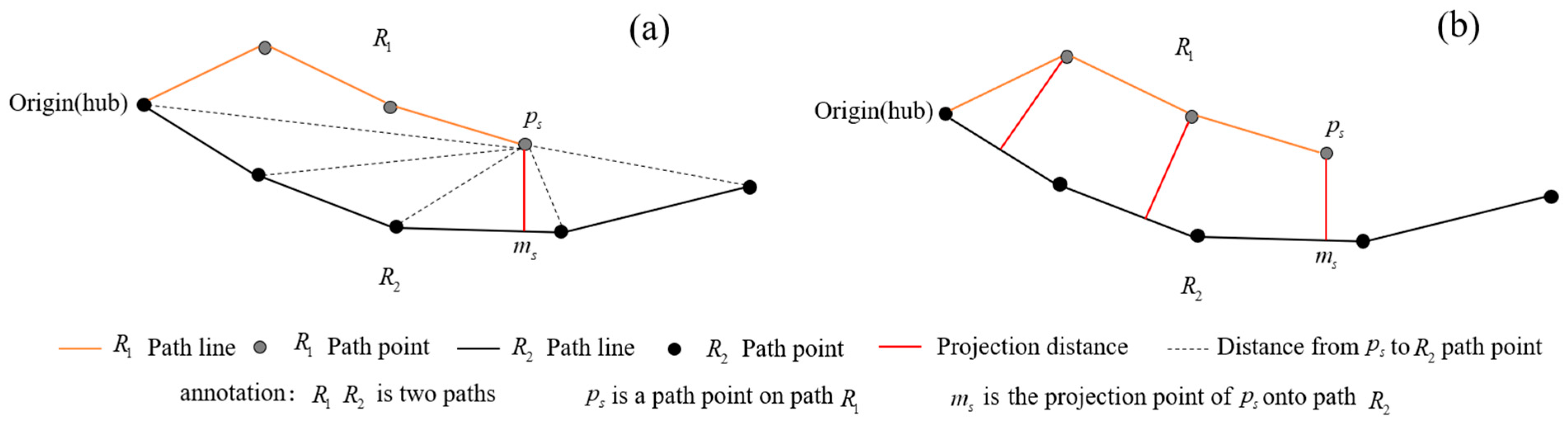
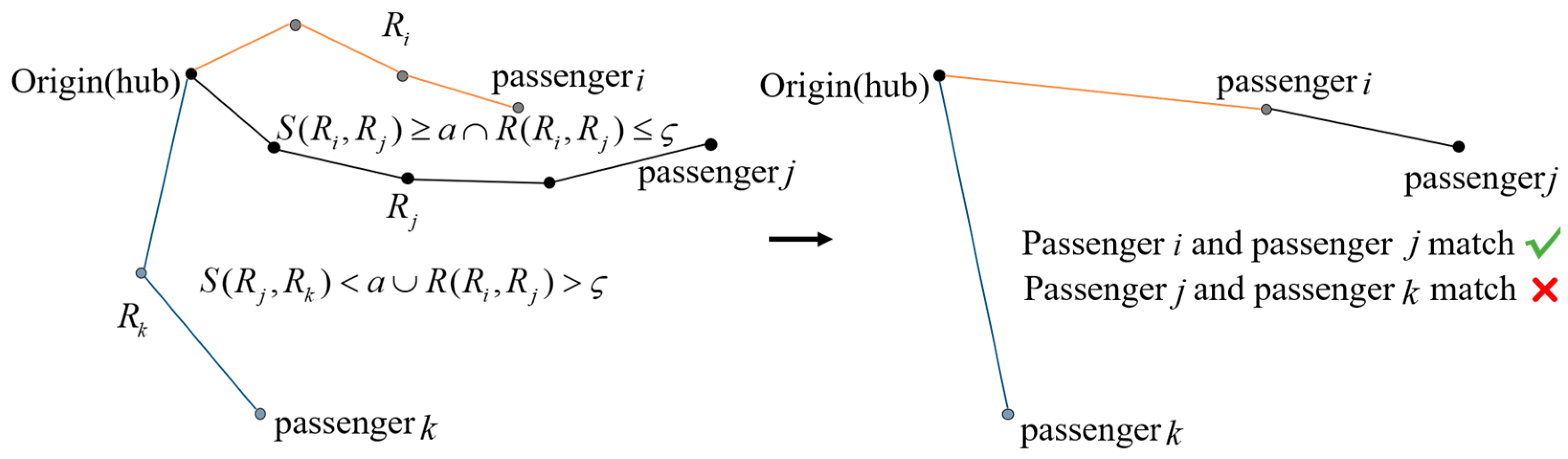
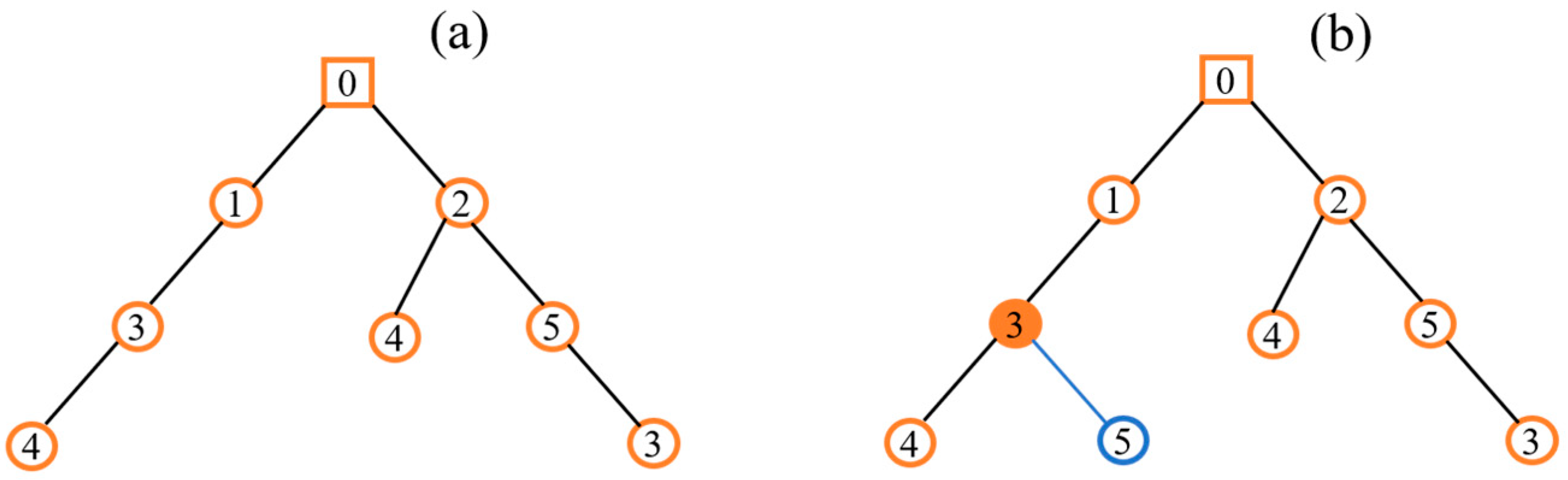
3.2.2. Measurement of Path Similarity

To measure the similarity of ridesharing paths under known origin–destination (OD) pairs, we propose a path similarity measurement method called the directionally corrected segment path distance (DSPD), which integrates spatial proximity and directional similarity. The DSPD metric incorporates both directional and positional characteristics, effectively reducing the impact of variations in path length and accurately assessing the similarity of path morphology (that is, driving trajectory similarity) despite variations in passengers’ destinations. Additionally, to reduce computational complexity and avoid analyzing all possible matching combinations individually, the model evaluates the similarity of traveling path morphology under paired OD pairs, using this as a key criterion for passenger matching.

(1)

Measurement of spatial proximity of paths

Definition 1. 

Projected distance from a point to a path (PD). The projected distance from a point to a path refers to the shortest distance from a point to a path [36], expressed as follows:

$${\mathrm{d}}_{PD}(p,R)=\min d_{\min }(p,r_s),\forall r_s\in R$$

(1)

where $p$ represents a point on the path; $R$ denotes a path; $r_s$ refers to a sub-segment of a path; and $d_{\min }(p,r_s)$ indicates the shortest distance from the point $p$ to the segment $r_s$. As illustrated in Figure 1a, the red line represents the projected distance from point $p_s$ on one path to another path $R_2$, where $m_s$ is the projection point of $p_s$ onto path $R_2$.

Definition 2. 

Segmented path distance (SPD). The segmented path distance refers to the average of the projected distances from points on one path to another path [36]. The calculation formula is as follows:

$$d_{SPD}(R_1,R_2)={\displaystyle \frac{1}{n_1}}{\displaystyle \sum _{p_s\in R_1}{d}_{PD}}(p_s,R_2)$$

(2)

where $R_1$ and $R_2$ represent two paths, $p_s$ represents a trajectory point on $R_1$,$n_1$ is the total number of trajectory points on path $R_1$, and $d_{PD}(p_s,R_2)$ is the projected distance from point $p_s$ on path $R_1$ to path $R_2$. Figure 1b shows an example of the SPD calculation.

Based on the above definitions, the DSPD evaluates the spatial proximity of two paths by calculating the average of projected distances from points on one path to another. This method effectively captures the overall proximity, thereby mitigating the impact of noise points. In this study on ridesharing at transport hubs, the destination requests of passengers are highly dispersed, resulting in paths of varying lengths. To measure the proximity between two paths of different lengths, we apply the minimum SPD as the metric of spatial proximity between the two paths, defined as follows:

$$D_s(R_1,R_2)=\min \left\{d_{SPD}(\right.R_1,R_2),\left.d_{SPD}(R_2,R_1\right\}$$

(3)

where $d_{SPD}(R_1,R_2)$ denotes the SPD from path $R_1$ to path $R_2$, and $d_{SPD}(R_2,R_1)$ represents the SPD from path $R_2$ to path $R_1$.

As defined in Equation (3), when paths vary in length, the minimum SPD is used to measure spatial proximity, focusing on the similarity of sub-path segments with the same length, as illustrated in Figure 1.

(2)

Measurement of directional similarity of paths

Definition 3. 

Directional vector discrepancy (DD). The directional vector discrepancy refers to the angular difference between the vector ${\lambda }_{1s}$ formed by point $p_{1s}$ and the subsequent point $p_{1s+1}$ on one path $R_1$ and the vector ${\lambda }_{2s}$ formed by point $p_{2s}$ and the subsequent point $p_{2s+1}$ on another path $R_2$. The calculation is as follows:

$$d_{PA}({\lambda }_{1s},{\lambda }_{2s})=1-{\displaystyle \frac{{\lambda }_{1s}·{\lambda }_{2s}}{\left|{\lambda }_{1s}\right|\left|{\lambda }_{2s}\right|}}$$

(4)

where $d_{PA}({\lambda }_{1s},{\lambda }_{2s})$ represents the directional vector discrepancy between the vector ${\lambda }_{1s}$ on path $R_1$ and the vector ${\lambda }_{2s}$ on path $R_2$. If $R_1$ is longer than $R_2$, then each of the remaining vectors is computed with the last vector in $R_2$. Figure 2 shows an example of the DD calculation.

Definition 4. 

Average directional vector discrepancy (ADD). The average directional vector discrepancy refers to the mean angular difference between the set of vectors formed by all the points on one path and the set of vectors formed by all the points on another path, expressed as follows:

$$d_{RA}(R_1,R_2)={\displaystyle \frac{1}{n_1-1}}{\displaystyle \sum _{s\in n_1-1}{d}_{PA}({\lambda }_{1s},{\lambda }_{2s})}$$

(5)

in this formula, $n_1$ − 1 denotes the total number of vectors derived from trajectory points on path $R_1$, and $d_{RA}(R_1,R_2)$ represents the directional difference in path $R_1$ relative to path $R_2$.

Thus, the overall directional similarity between paths $R_1$ and $R_2$ can be determined:

$$D_a(R_1,R_2)=\min \left\{d_{RA}(\right.R_1,R_2),\left.d_{RA}(R_2,R_1\right\}$$

(6)

where $d_{RA}(R_1,R_2)$ represents the directional difference in path $R_1$ relative to path $R_2$, and $d_{RA}(R_2,R_1)$ indicates the directional difference in path $R_2$ relative to path $R_1$. The value of $D_a$ ranges from 0 to 2, with values closer to 0 indicating a higher degree of overall directional similarity between paths $R_1$ and $R_2$.

(3)

Measurement of path similarity—DSPD

In this study on ridesharing at high-speed railway hubs, passengers share the same starting point, and each path’s direction significantly impacts the final path’s deviation. Thus, the path similarity measure integrates a directional correction, embedding directional similarity as an influencing factor within the spatial proximity metric. This approach results in a direction-corrected path similarity measure formulated as follows:

$$DSPS(R_1,R_2)={\displaystyle \frac{2}{2-D_a(R_1,R_2)}}·D_s(R_1,R_2)$$

(7)

where $DSPS(R_1,R_2)$ denotes the DSPD between paths $R_1$ and $R_2$, $D_s(R_1,R_2)$ represents spatial proximity, and $D_a(R_1,R_2)$ indicates directional similarity between the two paths. The value of $D_a(R_1,R_2)$ ranges from $[0,2]$. $2/2-D_a(R_1,R_2)$ acts as a correction factor for directional similarity, with $2/2-D_a(R_1,R_2)$ equal to 1 when the paths are identical, allowing the DSPD to capture spatial proximity fully. When the paths are entirely dissimilar, $2/2-D_a(R_1,R_2)$ becomes infinite, maximizing the distinction between two paths with different directions.

By applying the Gaussian function to standardize the DSPD, the path similarity measure is obtained as follows:

$$S(R_1,R_2)=\left\{\begin{array}{l}{\displaystyle \frac{\exp [-DSPD{(R_1,R_2)}^2]}{2{\sigma }^2}},D_a(R_1,R_2)\in [0,2)\\ {\displaystyle \frac{1}{M}},D_a(R_1,R_2)=2\end{array}\right.$$

(8)

where $S(R_1,R_2)\in (0,1)$ represents the normalized path similarity measure, and as $S(R_1,R_2)$ nears 1, path similarity increases. However, normalizing with a Gaussian function can distort the data when directional similarity is infinite. To address this, when directional similarity is infinite, $M$ is set to a significant value to ensure that when the paths are entirely dissimilar, the path similarity is 0.

The DSPD method ensures path similarity for passengers in a ridesharing state. To further guarantee the degree of detours in single-occupancy statuses, assume $L(R_1)<L(R_2)$, the detour between the endpoints of routes $R_1$ and $R_2$, represented by $R(R_1,R_2)$, must satisfy the maximum acceptable detour rate $\varsigma$ for single-occupancy trips.

$$R(R_1,R_2)={\displaystyle \frac{r(z_1,z_2)}{r(z_1^{\prime },z_2)}}\le \varsigma$$

(9)

where $z_1$ and $z_2$ represent the endpoints of routes $R_1$ and $R_2$, while $z_1^{\prime }$ signifies the point on route $R_2$ that corresponds to the same position as endpoint $z_1$. $r(z_1,z_2)$ and $r(z_1^{\prime },z_2)$ denote the path lengths (actual travel distances) from $z_1$ to $z_2$ and $z_1^{\prime }$ to $z_2$, respectively, as illustrated by the red line segments in Figure 3.

Figure 4 illustrates an example of passenger matching and the subsequent path updates following these rules:

1)

$S(R_i,R_j)\ge a\cap R(R_i,R_j)\le \varsigma$, where passenger $i$ and passenger $j$ achieve a successful match, $R_{0j}=R_{0i}+R_{ij}$;

2)

$S(R_j,R_k)<a\cup R(R_i,R_j)>\varsigma$, where passenger $i$ and passenger $j$ fail to match.

3.2.3. Mathematical Model

To alleviate peak-hour demand pressure and reduce operational costs for car service providers, we aim to optimize for the shortest total vehicle mileage and the fewest service vehicles. Concurrently, to meet passenger expectations, we develop a ridesharing model that considers route similarity.

$$\min Z={\displaystyle \sum _{i\in N_0}{\displaystyle \sum _{j\in N_0}{\displaystyle \sum _{k\in K}{c}_f}}{x}_{ijk}+{\displaystyle \sum _{i\in N_0}{\displaystyle \sum _{j\in N_0}{\displaystyle \sum _{k\in K}{c}_d}}}}{d}_{ij}{x}_{ijk}$$

(10)

$${\displaystyle \sum _{j\in N_0\cup j\ne i}{\displaystyle \sum _{k\in K}{x}_{ijk}}}=1,\forall i\in N_0$$

(11)

$${\displaystyle \sum _{i\in N_0\cup j\ne i}{\displaystyle \sum _{k\in K}{x}_{ijk}}}=1,\forall j\in N$$

(12)

$${\displaystyle \sum _{j\in N}{x}_{0jk}}=1,\forall k\in K$$

(13)

$${\displaystyle \sum _{i\in N}{x}_{i0k}}=0,\forall k\in K$$

(14)

$${\displaystyle \sum _{i\in N_0}{x}_{ijk}}={\displaystyle \sum _{l\in N_0}{x}_{jlk}},\forall j\in N,k\in K$$

(15)

$${\displaystyle \sum _{i\in N}(p_i+\max \left\{0,\left.⌈\frac{b_i-B}{W}⌉\right\}\right.){\displaystyle \sum _{j\in N}{x}_{ijk}}}\le Q,\forall k\in K$$

(16)

$$e_i\le \max \left\{e_i\right.x_{ijk}|e_i{x}_{ijk}\ne 0,\forall i,j\in \left.N\right\}\le l_i,k\in K$$

(17)

$$\begin{array}{c}e{e}_i\le \max \left\{e_i\right.x_{ijk}|e_i{x}_{ijk}\ne 0,\forall i,j\in \left.N\right\}\\ +{\displaystyle \sum _{i\in N}{\displaystyle \sum _{j\in N}{x}_{ijk}}}({\displaystyle \frac{d_{ij}}{v}}+s)\le l{l}_i,k\in K\end{array}$$

(18)

$$S({\displaystyle \sum _{i\in N_0}{\displaystyle \sum _{j\in N}{x}_{ijk}{R}_{0j}}},{\displaystyle \sum _{i\in N_0}{\displaystyle \sum _{l\in N}{x}_{ilk}{R}_{0l}}})\ge a,k\in K$$

(19)

$$R({\displaystyle \sum _{i\in N_0}{\displaystyle \sum _{j\in N}{x}_{ijk}{R}_{0j}}},{\displaystyle \sum _{i\in N_0}{\displaystyle \sum _{l\in N}{x}_{ilk}{R}_{0l}}})\le \varsigma ,k\in K$$

(20)

$$x_{ijk}\in \left\{0,\left.1\right\}\right.,\forall i,j\in N_0,k\in K$$

(21)

The objective function (10) minimizes overall system costs, including total vehicle mileage and the number of vehicles required for service. Constraints (11) and (12) ensure that each request is served precisely once. Constraints (13) and (14) guarantee that all cars depart from the hub and do not return during the service. Constraint (15) ensures traffic flow balance. Constraint (16) is a capacity limitation, ensuring that the total number of passengers and luggage does not exceed the vehicle’s carrying capacity. Constraints (17) and (18) indicate time windows: Constraint (17) dictates that the latest arrival time for passengers sharing the exact vehicle aligns with the car’s departure time, which must meet each passenger’s departure window; Constraint (18) ensures that every passenger’s arrival time falls within the designated arrival window. Constraint (19) requires that passengers sharing the same car have path similarities that meet a specified threshold. ${\displaystyle \sum _{i\in N_0}{\displaystyle \sum _{j\in N}{x}_{ijk}{R}_{0j}}}$ and ${\displaystyle \sum _{i\in N_0}{\displaystyle \sum _{l\in N}{x}_{ilk}{R}_{0l}}}$ represent the routes from the hub 0 to points $j$ and $l$ before ridesharing. Constraint (20) stipulates that the detour between the destinations of passengers sharing the same car must meet the detour rate $\varsigma$. Equation (21) defines the decision variable as a 0–1 integer constraint.

4. Solution Algorithm

Ridesharing at high-speed railway hubs differs from road network ridesharing; here, passengers have the same starting point, making it unable to match riders based on the original car routes, resulting in an extensive set of possible vehicle matching combinations. Consequently, we propose a tailored PVS-ALNS heuristic algorithm that combines path vector similarity-based (PVS) heuristic clustering and an adaptive large neighborhood search algorithm (ALNS). The PVS heuristic clustering is designed to group requests with similar traveling paths, decomposing the large-scale VRP into smaller sub-problems. Subsequently, the ALNS algorithm is applied to determine the optimal ridesharing routes for each cluster.

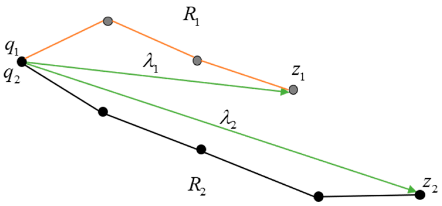
4.1. Request Clustering Based on Path Vector Similarity

Traveling path and ride time are critical factors influencing passenger matching. In the context of ridesharing at high-speed railway hubs, passengers share the same starting point, and the direction of their routes plays a decisive role in determining the traveling path. In contrast, the distance between passengers’ destinations has a relatively minor impact on the “near-to-far” travel pattern discussed in this study. Accordingly, this section proposes a path vector similarity measurement method incorporating directional and temporal characteristics to cluster passengers with similar route directions and minimal time spans into the same group.

4.1.1. Definition of Path Vector Similarity

Without participating in ridesharing, requests $r_1$ and $r_2$ can result in two separate paths, $R_1$ and $R_2$, departing from the large transport hub. Taking the starting points $q_1$ and $q_2$ and the endpoints $z_1$ and $z_2$ of the two paths, the vectors ${\lambda }_1$ and ${\lambda }_2$ are obtained by connecting the starting and ending points, as shown in Figure 5.

(1)

Vector similarity in direction

We calculate the cosine of the intersection angle between the vectors ${\lambda }_1$ and ${\lambda }_2$, obtained from the start and end points of the two paths, denoted as $\cos 〈{\lambda }_1,{\lambda }_2〉$. If $\mu \le \cos 〈{\lambda }_1,{\lambda }_2〉\le 1$, the two vectors are considered directionally similar, expressed as follows:

$$VD(R_1,R_2)=\left\{\begin{array}{l}1,\mu \le \cos 〈{\lambda }_1,{\lambda }_2〉\le 1\\ -N,\cos 〈{\lambda }_1,{\lambda }_2〉<\mu \end{array}\right.$$

(22)

where $VD(R_1,R_2)$ denotes the directional similarity between the two paths, and $N$ represents a significantly large constant.

(2)

Vector similarity in temporal

We consider the temporal attribute, which pertains to the departure window from the hub, stipulating that passengers with overlapping departure windows have the potential to be matched. The longer the overlap, the greater the likelihood of a successful match. For any two passenger requests, with time attributes $t_1$ and $t_2$, the temporal similarity between paths $R_1$ and $R_2$ is calculated as shown in Equation (23):

$$VT({\mathrm{t}}_1,t_2)=\left\{\begin{array}{l}|\min \left\{l_1\right.,\left.l_2\right\}-\max \left\{e_1\right.,\left.e_2\right\}|,if\min \left\{l_1\right.,\left.l_2\right\}>\max \left\{e_1\right.,\left.e_2\right\}\\ 0,otherwise\end{array}\right.$$

(23)

In the hub ridesharing problem context, the direction of travel paths is decisive in determining shared routes. Consequently, directional similarity is incorporated into the temporal similarity metric as an influencing factor. The expression for the path vector similarity measurement method is as follows:

$$VDT(R_1,R_2)=VD(R_1,R_2)·VT(R_1,R_2)$$

(24)

where $VDT(R_1,R_2)$ represents the path vector similarity between paths $R_1$ and $R_2$, $VD(R_1,R_2)$ denotes the directional similarity between the two vectors, and $VT(R_1,R_2)$ indicates the temporal similarity between the paths.

4.1.2. Clustering Based on a Greedy Heuristic Algorithm

Ref. [33] have demonstrated that, in most ride-sharing scenarios, a greedy algorithm achieves better clustering results than the K-Means method. Therefore, in this section, using path vector similarity (PVS) as the benchmark, a greedy heuristic algorithm is employed for clustering. This approach groups similar passengers into the same cluster based on the similarity of their route directions and temporal spans.

4.2. Adaptive Large Neighborhood Search Algorithm

After clustering, each cluster requires matching and optimization. Considering the complex constraint of path similarity in our model, there is a significant reliance on trajectory data, making it difficult to directly use off-the-shelf solvers (for instance, CPLEX and GUROBI). Adaptive large neighborhood search (ALNS) algorithms are highly effective at accommodating the complex constraints of VRP-related problems. Therefore, we design an algorithm based on the ALNS framework. Algorithm 1 outlines the main steps of the ALNS, including initial solution generation, removal and repair operators, and their adaptive selection using a roulette wheel strategy [37]. To avoid local optima during the search, we apply the Metropolis criterion [37] to accept new solutions. The parameter $T_0$ represents the initial temperature of the algorithm, and $\xi$ denotes the cooling rate; the algorithm terminates upon reaching the maximum iteration count.

Algorithm 1: Outline of ALNS
01	Input: similarity data, removal and repair operators, other algorithm
02	$\mathrm{Output}: \mathrm{the} \mathrm{best} \mathrm{solution} (S_{best}$)
03	current an initial solution by Insert algorithm
04	$\mathrm{set} S_{best}$$\leftarrow S_{\mathrm{new}}$$, S_{curr}$$\leftarrow S_{new}$, iter ← 0;
05	while termination criteria are not met do
06	select removal & repair operators by roulette selection
07	$S_{temp}$$\leftarrow \mathrm{removal} \mathrm{and} \mathrm{repair} (S_{curr}$)
08	$\mathrm{if} f(S_{temp}$$) > f(S_{best}$)
09	$S_{best}$$\leftarrow S_{curr}$$\leftarrow S_{temp}$$, \mathit{iter}=0, \mathrm{and} \mathrm{update} \mathrm{operator} \mathrm{scores} \mathrm{by} {\omega }_1$
10	$\mathrm{else} \mathrm{if} f(S_{temp}$$) > f(S_{curr}$)
11	$S_{curr}$$\leftarrow S_{temp}$$,\mathit{iter}=0, \mathrm{and} \mathrm{update} \mathrm{operator} \mathrm{scores} \mathrm{by} {\omega }_2$
12	$\mathrm{else} \mathrm{if} f(S_{temp}$$\le$$f(S_{curr}$) but accepted by the Metropolis criterion then
13	$S_{curr}$$\leftarrow S_{temp}$$,\mathit{iter}+1, \mathrm{and} \mathrm{update} \mathrm{operator} \mathrm{scores} \mathrm{by} {\omega }_3$
14	else
15	$\mathrm{reject} \mathrm{solution}, \mathit{iter}+1, \mathrm{and} \mathrm{update} \mathrm{operator} \mathrm{scores} \mathrm{by} {\omega }_4$
16	update T, scores, and weights of removal & repair operators
17	$\mathrm{return} S_{best}$

4.2.1. Initial Solution

We employ a random insertion algorithm to construct the algorithm’s initial solution. An empty route is created, and unvisited requests are inserted into this route individually. Subsequently, the feasibility of inserting request $i$ into the route $r$ is evaluated. Based on the feasibility assessment, request $i$ is either inserted into the route $r$ or used to construct a new empty path. Algorithm 2 details the complete procedure for building this initial solution.

Algorithm 2: Insert algorithm
01	Input: requests, cars
02	Output: set of routes
03	uninserted requests ← all requests
04	while |uninserted requests| > 0 do
05	generate a new empty route (r)
06	for each request do
07	for each possible insertion position in the route do
08	new route ← insert the request at the current position
09	check the feasible of the new route;
10	if the new route is feasible then
11	delete this uninserted requests, r ← new route and break
12	else
13	try inserting in the next position
14	add r to routes
15	return routes

4.2.2. Removal and Repair Operators

Three removal and repair operators are designed to obtain the optimum solution.

(1)

Random Removal: This operator randomly removes a certain number of requests from the current vehicle route at a specific rate of destruction.

(2)

Worst removal: This operator removes the request, saving the most considerable routing cost. First, the routing cost savings are calculated for each request removed. Then, the request that results in the most significant cost savings is removed from the current route. Finally, the first two steps are repeated until the number of removals is satisfied.

(3)

Shaw Removal: We define the similarity of two requests in a route, obtain the two requests with the highest similarity, and remove one request from it to increase the diversity of the scheme. The similarity of two requests i and j for a route is defined as SM(i,j), as shown in Equation (25).

$$SM(i,j)=\epsilon \times |e_i-e_j|+\upsilon \times |l_i-l_j|+\omega \times [1-ccmat(i,j)]$$

(25)

where $e_i-e_j$ represents the difference in earliest departure times, $l_i-l_j$ denotes the difference in latest departure times, and $1-ccmat(i,j)$ indicates the difference in similarity between the two paths. The weights $\epsilon$, $\upsilon$, and $\omega$ are all set to 0.5, respectively.

After the removal operation, the vehicle route and the removal request are obtained. Next, we use the repair operator to insert the removal request into the vehicle routing scheme.

(1)

Random Repair: Each request can be randomly inserted into a feasible location. An empty route is created to insert this request if no feasible position exists.

(2)

Greedy Repair: This operator first calculates the insertion cost of inserting each request into each available location and then selects the request–location pair that results in the smallest increase in routing cost, which means this request will be inserted into this position. If there is no feasible insertion location for a given request, an empty route is generated for storage.

(3)

Regret-2 Repair: This operator includes a forward-looking message when selecting a customer to insert. We use $\Delta C_i^r$ to denote the minimum insertion cost of placing a request $i$ into route $r$. This operator calculates the insertion costs $\Delta C_i^r$ of placing the request into the first-best and second-best routes. $RV(i)=\Delta C_i^{r(2)}-\Delta C_i^{r(1)}$ represents the maximum regret value for inserting the request $i$. The request with the highest regret value is inserted into the first-best position.

4.2.3. Adaptive Mechanism

To select the removal and repair operators more efficiently, we select and adjust them at each iteration based on their weights and the roulette wheel. Each operator’s weight is determined by its performance in previous iterations. Initially, each operator’s weight is set to 1, and during each iteration, weights are updated according to Equation (26).

$$w_i=\left\{\begin{array}{l}(1-U)w_i+U{\displaystyle \frac{s_i}{t_i}},t_i>0\\ w_i,t_i=0\end{array}\right.$$

(26)

where $s_i$ is the score of the operator $i$ recorded in the previous iteration, $t_i$ is the number of times operator $i$ was selected in the last stage, and $U\in [0,1]$ is the response factor that controls the speed of weight adjustment. In each iteration, the removal and repair operators determine a score based on the quality of the new solution. The initial score is set to 0; if the temporary solution outperforms the global optimal solution, the removal and repair operator score increases by ${\omega }_1$. If the temporary solution is inferior to the global optimal solution but better than the current solution, the removal and repair operator score increases by ${\omega }_2$. If the temporary solution is worse than the global optimum yet still accepted, the removal and repair operator scores increase by ${\omega }_3$. If the temporary solution is worse than the global optimal solution but not accepted, the removal and repair operator scores increase by ${\omega }_4$.

4.2.4. Parallel Computing and Acceleration Strategies

Parallel computing tackles large-scale problems that can be decomposed into multiple independent subproblems. Solving each subproblem in parallel significantly accelerates the overall solution process. This study first segments large-scale requests into independent vehicle request clusters using PVS-based heuristic clustering. These clusters are processed independently, with the parallel computing framework illustrated in Figure 6.

Numerous identical neighboring solutions may arise in the neighborhood search process. To quickly identify duplicates and prevent redundant calculations, we employ a trie structure to track information on previously examined paths, a proven effective strategy in alleviating time-consuming feasibility checks and computational issues [38,39].

In this study, we use a trie structure to store route request IDs in conjunction with the total cost of each route. To minimize the trie’s storage footprint, we specify that if a route is feasible, the cost value returns as the total route cost; if infeasible, the cost returns as infinity. Two cases are distinguished as follows:

(1)

When a complete route is successfully retrieved, return the total cost of the route directly.

(2)

When a complete route is not retrieved, assess its feasibility, calculate the total cost, and store it in the trie structure.

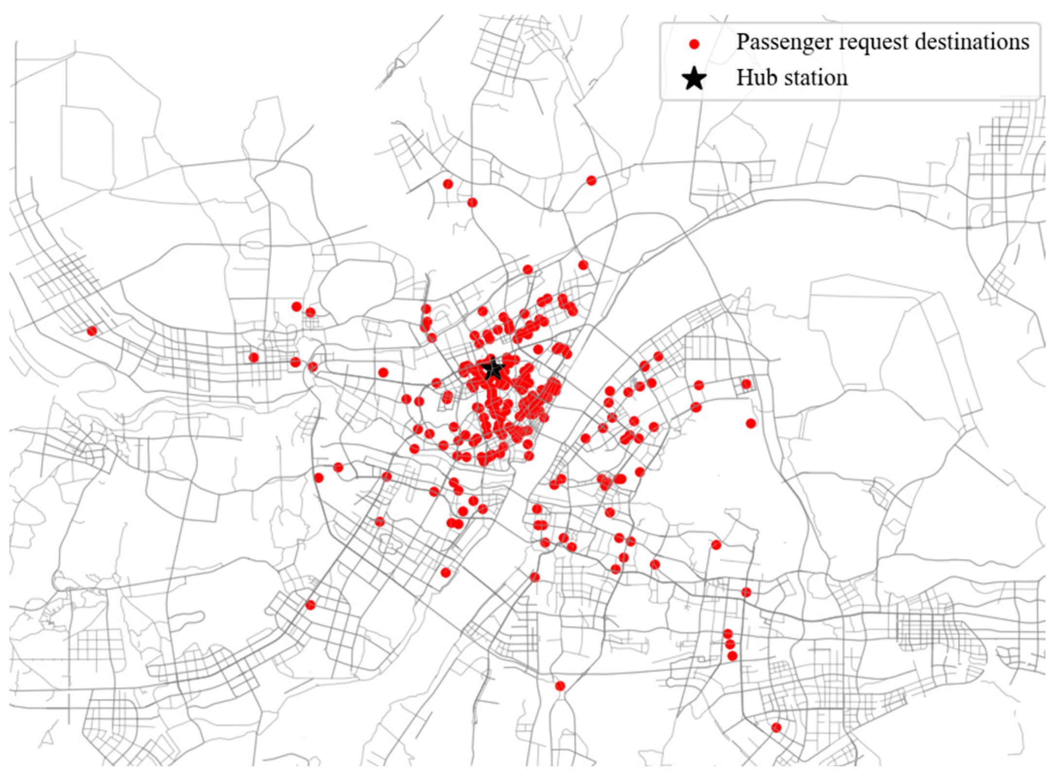
Figure 7 illustrates the retrieval and storage of routing information. In Figure 7a, the current trie contains four routing entries: (0–1–3), (0–2–4), (0–1–3–4), and (0–2–5–3). If the new route to be evaluated is (0–2–5–3), we can directly obtain the total cost of this route from the trie. For the new route (0–1–3–5), which is not stored in the trie, we need to recalculate its associated information and store it in the trie, as shown in Figure 7b.

5. Case Study

In this experiment, we utilize real taxi data from Wuhan, China, focusing on Hankou Station as a high-speed railway hub. We selected order data from weekdays, which includes order IDs, start and end coordinates, and order start and end times (for example, Figure 8 shows the distribution of 230 passenger request destinations from Hankou Station between 22:00 and 23:00). The algorithm developed for this study is implemented in Python 3.9, and all simulations are executed on a PC equipped with 64 GB RAM and a 3.4 GHz CPU.

5.1. Parameter Configuration and Instance Generation

The model parameters are as follows: the fixed usage cost $c_f$ = USD 2.77, and the driving cost per kilometer $c_d$ = 1. The number of pieces of luggage that can be placed on the trunk $B$ = 2; the number of pieces of luggage that can be placed on a seat $W$ = 2. The speed of the vehicle $v$ = 40 km/h. Drop-off time at each service point $s$ = 0.2 min. The maximum acceptable detour rate $\varsigma$ = 1.5 for single-occupancy status.

The solution algorithm parameters are as follows: in the PVS-based heuristic clustering algorithm, the maximum cosine value between two vector angles $\mu$ = 0.5. In the ALNS algorithm, the initial temperature $T_0$ is 100, the cooling rate $\xi$ = 0.97, the weight update reaction factor $U$ = 0.5, and the maximum number of iterations $M$ is 100. Operator scores are ${\omega }_1$ = 1.5, ${\omega }_2$ = 1.2, ${\omega }_3$ = 0.8, and ${\omega }_4$ = 0.6, respectively.

Regarding instance generation, the departure time window $e_i$ is based on the order start time, derived from an analysis of real taxi operational data in Wuhan. The passenger waiting time is randomly generated within a range of [5,15] minutes. The arrival time window is defined by $[e_i+d_{ij}/v+s,{\mathrm{l}}_i+\gamma (d_{ij}/v+s)]$, where $\gamma$ = 1.5 represents the maximum acceptable detour rate for passengers. Next, we randomly generate the number of riders and the amount of large luggage for each request. The number of riders is either 1 or 2, with probabilities of 80% and 20%, respectively, while large luggage amounts are 0, 1, or 2, with probabilities of 50%, 40%, and 10% [1]. Based on the origin and destination data from car orders, we utilized the OSRM routing engine to generate routes and calculate the distances between all requests. We obtained trajectory points at 100 m intervals along the path.

5.2. Analysis of the Effects of Heuristic Clustering Based on Path Vector Similarity

The ride-sharing model presented in this paper can be solved using a solver without considering the constraint of route similarity. However, introducing DSPD requires measuring the spatial proximity and angular similarity of routes, which heavily relies on route trajectories, making it difficult to solve directly using a standard solver.

To evaluate the computational performance of the proposed algorithm, we compare the solution results of the PVS-ALNS algorithm with those directly using the ALNS algorithm by using taxi passenger request data at different times and scales.

Table 2. Comparison of passenger case optimization results.

Scale	Index	PVS-ALNS	ALNS	Gap (%)
60	Objective function/USD	131.87	131.87	0
	Number of cars/vehicles	28	28	0
	Total car mileage/km	381.92	381.92	0
	Average solution time/s	28.31	139.85	79.8
	Average passenger waiting time/minute	3.07	3.07	0
120	Objective function/USD	304.40	308.16	1.2
	Number of cars/vehicles	52	52	0
	Total car mileage/km	989.35	1014.37	2.5
	Average solution time/s	42.23	711.65	94
	Average passenger waiting time/minute	2.87	4.14	30.6
230	Objective function/USD	401.45	406.35	1.2
	Number of cars/vehicles	71	71	0
	Total car mileage/km	1483.38	1526.71	2.8
	Average solution time/s	86.24	1882.40	95
	Average passenger waiting time/minute	2.90	4.16	30.2

presents the average results of 10 runs for both algorithms. It can be found that the two-stage algorithm in this paper achieves the same optimization results as the global optimization method in the scenario with a small data scale, but in the scenario with a large data scale, the proposed method obtains better optimization results with the same number of iterations. When the data scale is 230, the calculation time of the algorithm is reduced by more than 95%, and the average passenger detour ratio and average passenger waiting time are reduced by 4% and 30%, respectively. This demonstrates that the clustering method proposed in this study effectively groups similar passenger requests, improving computational efficiency while ensuring optimization quality, thereby achieving the goal of rapidly matching large-scale passenger requests at a high-speed railway hub.

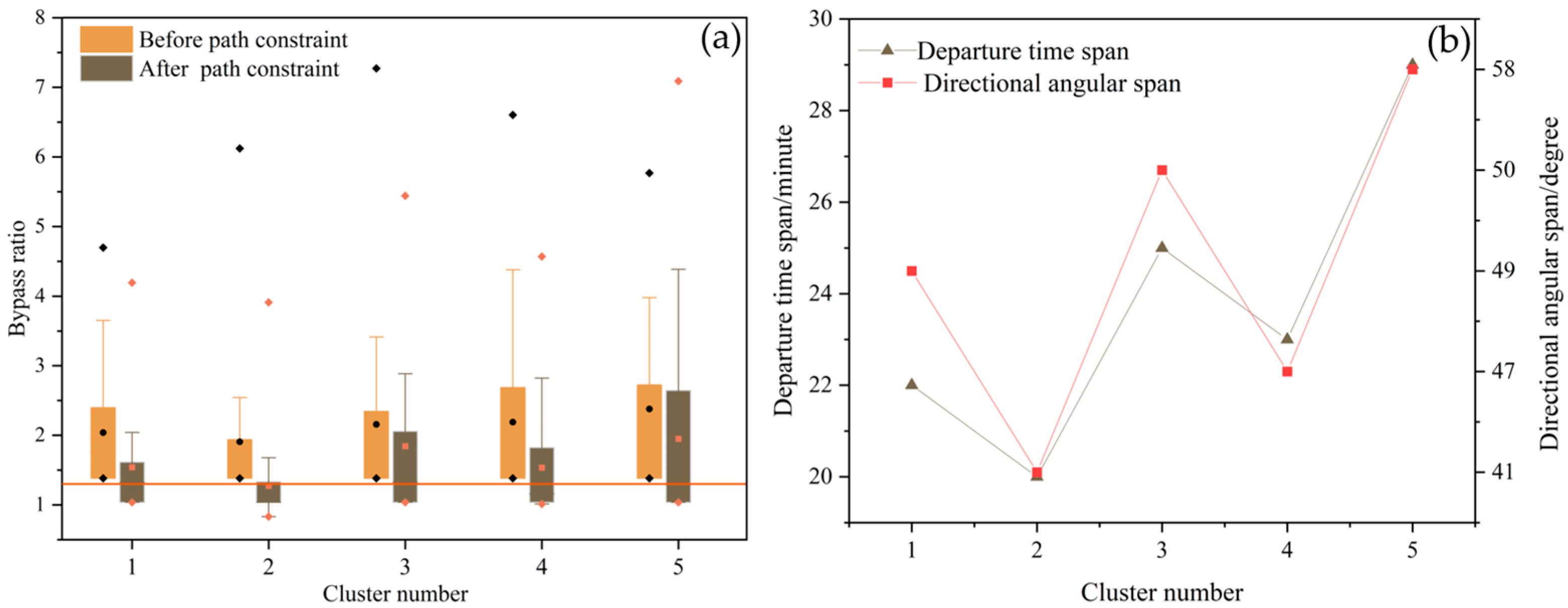
5.3. Analysis of the Effects of Path Similarity

To examine the impact of incorporating path similarity as a constraint, we analyze from perspectives including vehicle count, mileage savings, and detour ratios under 230 requests. Figure 9 presents the box plot of detour ratios when the threshold is set to 0.8 and the line charts of directional angles and departure time span of passenger requests within clusters. Considering path similarity constraints, the overall detour ratio decreases, with the proportion of passengers experiencing a detour ratio below 1.3 increasing from 42% to 60%. This indicates that the proposed method can effectively reduce passenger detour distances. Moreover, each cluster’s highest average detour ratio is Cluster 5, and the lowest is Cluster 2. Analyzing the directional angles and departure time spans of passenger requests within the clusters reveals that matching results are closely related to clustering characteristics: the smaller the directional angle and departure time span within a cluster, the better the matching performance, and vice versa.

Table 3. Overall result comparison considering route similarity.

Index	Before Ridesharing	With Path Constraints	Without Path Constraints
Objective function/USD	880.73	401.45	411.35
Total car mileage/km	1772.24	1483.38	1577.35
Number of cars/vehicles	230	71	70
Total mileage saving rate/%	—	16%	11%
Average passenger diversions ratio	—	1.56	1.84
Ridesharing success rate/ %	—	97%	100%
JAC value	—	0.63	0.52

indicates that with path constraints in place, the number of cars decreases from 230 pre-ridesharing to 71, achieving a ridesharing success rate of 97%; the total mileage savings reaches 16% and overall operational costs drop by 54%; and the average detour ratio for passengers is 1.56, showcasing significant cost and resource savings while ensuring a satisfactory passenger experience.

A comparison with the unconstrained model shows that removing path constraints slightly reduces car usage but leads to a nearly 6% increase in total mileage and raises the average passenger detour ratio to 1.84. Without path constraints, while ridesharing success rates can improve, total travel mileage and passenger detour ratios and operational costs for car service providers tend to increase.

The JAC index [40] aims to quantify the overlap of road segments, with the calculation formula being.

$$JAC(R,R^{\prime })={\displaystyle \frac{\left|\left\{\left.R_{\mathrm{edges}}\right\}\cap \left\{\left.R_{edges}^{\prime }\right\}\right.\right.\right|}{\left|\left\{\left.R_{\mathrm{edges}}\right\}\cup \left\{\left.R_{edges}^{\prime }\right\}\right.\right.\right|}}$$

(27)

The average JAC value under path constraints is 0.63, compared to 0.52 without constraints, indicating that ridesharing routes with constraints better align with passengers’ expectations regarding travel paths.

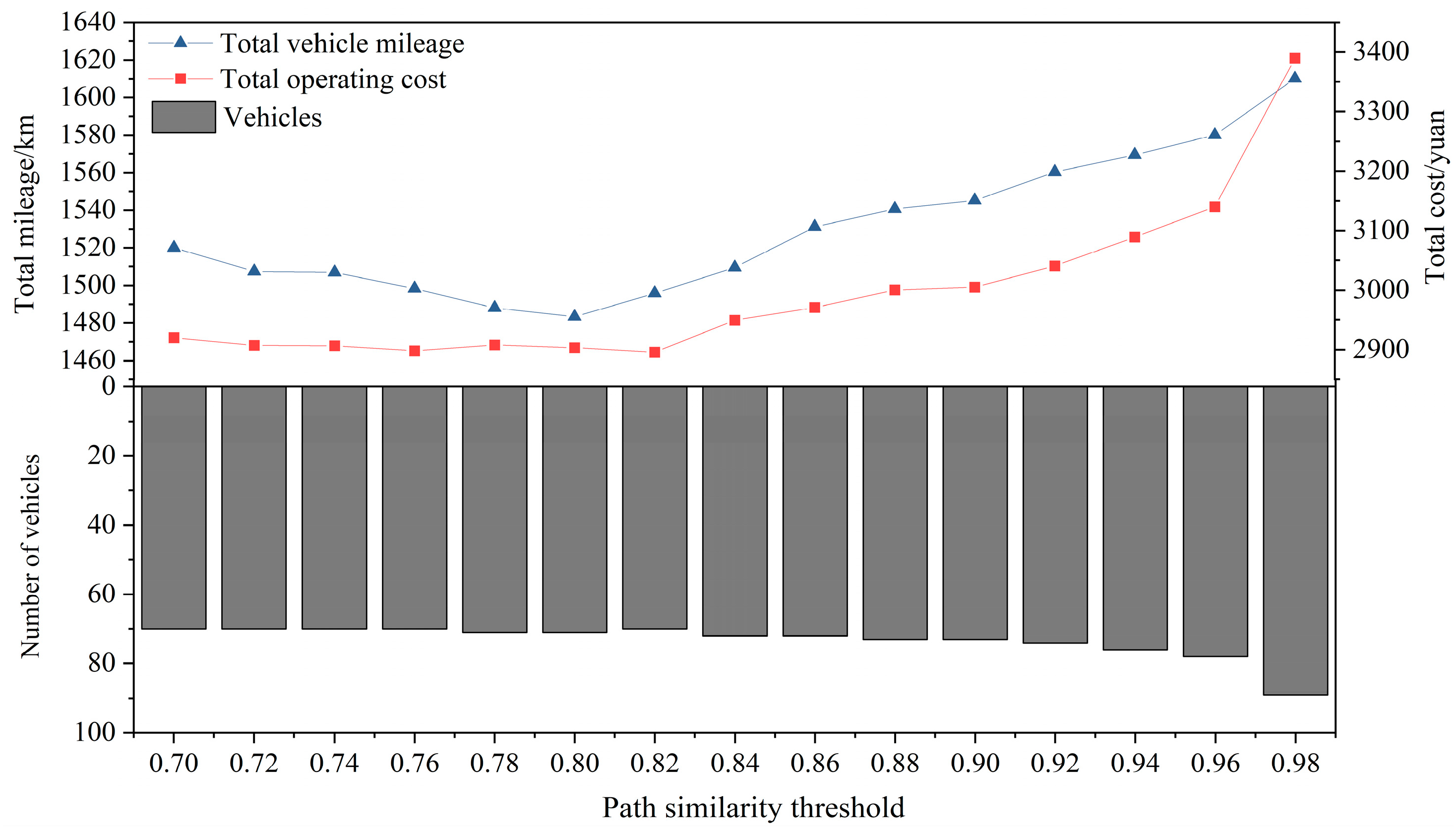
5.4. Sensitivity Analysis of Path Similarity Threshold

To investigate the impact of path similarity thresholds, we set the threshold value $a$ within a range of 0.7 to 0.98. The resulting total operating cost, vehicle miles traveled, and vehicle count are shown in Figure 10. It is observed that between threshold values of 0.7 and 0.82, vehicle numbers remain essentially unchanged. This stability results from preliminary request clustering via PVS, ensuring high path vector similarity among passengers in the same cluster, which enhances matching rates and ridesharing success. Furthermore, within this threshold range, when the threshold value $a$ is set to 0.8, the total vehicle miles traveled is minimized. This suggests that a specific threshold can effectively match requests with similar paths, making the algorithm achieve a better solution within the same computational time. When the threshold $a$ exceeds 0.82, stricter path similarity constraints reduce ridesharing success rates, leading to increased vehicle miles traveled and higher overall operating costs. When the threshold value $a$ is set between 0.78 and 0.82, the total vehicle mileage and overall target cost reach their lowest point. Therefore, within this range of values, it is possible to ensure a lower detour ratio while reducing the total operational cost.

5.5. Analysis of the Impact of Large Luggage on Route Feasibility

To illustrate the importance of considering large luggage in ridesharing services at a high-speed railway hub, we employ the Monte Carlo simulation method to analyze route feasibility without accounting for large luggage. First, using the random method for generating large luggage requests described in Section 5.1, we randomly select passengers with large luggage from 230 requests at different proportions, and the number of passengers per request is also randomly generated, as detailed in Section 5.1. Then, we construct ridesharing matches within a model that excludes large luggage considerations. Figure 11 shows the probability of route infeasibility across 1000 simulation trials. As observed, when the share of large luggage requests is low (for instance, under 10%), it has a minimal impact on route feasibility. Consequently, large luggage can be overlooked in ridesharing designs aimed at commuting or transport to bus and subway stations. However, route feasibility significantly impacts ridesharing at high-speed railway hubs, where a higher number of passengers carry large luggage. For instance, when more than 50% of passengers possess large luggage, the probability of route infeasibility exceeds 20%, indicating a considerable impact. Thus, it is essential to consider the influence of large luggage on route feasibility for ridesharing services at large rail hubs or airports.

6. Conclusions

We propose a ridesharing strategy to swiftly alleviate the high influx of arriving passengers at high-speed railway hubs. By incorporating route similarity constraints into the model, we ensure that the planned routes align with passenger expectations while accommodating their departure and arrival times and large luggage needs. The optimization seeks to minimize total vehicle mileage and the number of service vehicles, utilizing a two-stage PVS-ALNS algorithm for solutions.

The case study shows that: (1) for large-scale ridesharing optimization problems, the two-stage PVS-ALNS method improves computational efficiency by 95% while effectively reducing passengers’ waiting time and detour distances. (2) Sensitivity analysis shows that thresholds between 0.78 and 0.82 minimize total operational costs while maintaining low detour ratios. (3) It is found that under the path similarity constraint, the total mileage and operating cost of the vehicle can be effectively reduced, the proportion of passengers detouring is low, and the JAC value of the route after carpooling can be increased from 0.52 to 0.63. (4) In rideshare matching at high-speed railway hubs, the impact of large luggage must be considered to ensure compliance with car capacity constraints.

This study assumes that all passengers arrive at designated ridesharing points at high-speed railway hubs as scheduled. However, vehicle arrival delays and passengers’ unfamiliarity with the hub layout may impact when passengers arrive at these pickup points. Future research could consider ridesharing strategies that accommodate passenger delays, thus enhancing service flexibility.

References

1. He, P.; Jin, J.G.; Schulte, F.; Trépanier, M. Optimizing first-mile ridesharing services to intercity transit hubs. Transp. Res. Part C-Emerg. Technol. 2023, 150, 104082. [Google Scholar]
2. Nourinejad, M.; Roorda, M.J. Agent based model for dynamic ridesharing. Transp. Res. Part C-Emerg. Technol. 2016, 64, 117–132. [Google Scholar]
3. Bian, Z.Y.; Liu, X. Mechanism design for first-mile ridesharing based on personalized requirements part I: Theoretical analysis in generalized scenarios. Transp. Res. Part B-Methodol. 2019, 120, 147–171. [Google Scholar]
4. Li, Y.Y.; Liu, Y.; Xie, J. A path-based equilibrium model for ridesharing matching. Transp. Res. Part B-Methodol. 2020, 138, 373–405. [Google Scholar] [CrossRef]
5. Du, M.Q.; Zhou, J.K.; Li, G.Y.; Tan, H.Q.; Chen, A.T.Y. A stochastic ridesharing user equilibrium model with origin-destination-based ride-matching strategy. Transp. Res. Part E-Logist. Transp. Rev. 2024, 189, 103688. [Google Scholar]
6. Hosni, H.; Naoum-Sawaya, J.; Artail, H. The shared-taxi problem: Formulation and solution methods. Transp. Res. Part B-Methodol. 2014, 70, 303–318. [Google Scholar]
7. Yin, R.Y.; Lu, P.X. A Cluster-First Route-Second Constructive Heuristic Method for Emergency Logistics Scheduling in Urban Transport Networks. Sustainability 2022, 14, 2301. [Google Scholar] [CrossRef]
8. Nitter, J.; Yang, S.S.; Fagerholt, K.; Ormevik, A.B. The static ridesharing routing problem with flexible locations: A Norwegian case study. Comput. Oper. Res. 2024, 167, 106669. [Google Scholar]
9. Fielbaum, A. Optimizing a vehicle’s route in an on-demand ridesharing system in which users might walk. J. Intell. Transp. Syst. 2022, 26, 432–447. [Google Scholar]
10. Najmi, A.; Waller, T.; Liu, W.; Rashidi, T.H. Integration of ridesharing and activity travel pattern generation. Transp. A-Transp. Sci. 2023. [Google Scholar] [CrossRef]
11. Agatz, N.A.H.; Erera, A.L.; Savelsbergh, M.W.P.; Wang, X. Dynamic ride-sharing: A simulation study in metro Atlanta. Transp. Res. Part B-Methodol. 2011, 45, 1450–1464. [Google Scholar]
12. Ramezani, M.; Valadkhani, A.H. Dynamic ride-sourcing systems for city-scale networks- Part I: Matching design and model formulation and validation. Transp. Res. Part C-Emerg. Technol. 2023, 152, 104158. [Google Scholar]
13. Miller, J.; How, J.P. Predictive Positioning and Quality Of Service Ridesharing for Campus Mobility On Demand Systems. In Proceedings of the 2017 IEEE International Conference on Robotics and Automation (ICRA), Singapore, 29 May–3 June 2017; pp. 1402–1408. [Google Scholar]
14. Ma, J.; Xu, M.; Meng, Q.; Cheng, L. Ridesharing user equilibrium problem under OD-based surge pricing strategy. Transp. Res. Part B-Methodol. 2020, 134, 1–24. [Google Scholar]
15. Li, M.; Di, X.; Liu, H.X.; Huang, H.J. A restricted path-based ridesharing user equilibrium. J. Intell. Transp. Syst. 2020, 24, 383–403. [Google Scholar]
16. Hsieh, F.S. Trust-Based Recommendation for Shared Mobility Systems Based on a Discrete Self-Adaptive Neighborhood Search Differential Evolution Algorithm. Electronics 2022, 11, 776. [Google Scholar] [CrossRef]
17. Huang, Y.T.; Kockelman, K.M.; Garikapati, V. Shared automated vehicle fleet operations for first-mile last-mile transit connections with dynamic pooling. Comput. Environ. Urban Syst. 2022, 92, 101730. [Google Scholar]
18. Stiglic, M.; Agatz, N.; Savelsbergh, M.; Gradisar, M. Enhancing urban mobility: Integrating ride-sharing and public transit. Comput. Oper. Res. 2018, 90, 12–21. [Google Scholar]
19. Ma, T.Y.; Rasulkhani, S.; Chow, J.Y.J.; Klein, S. A dynamic ridesharing dispatch and idle vehicle repositioning strategy with integrated transit transfers. Transp. Res. Part E-Logist. Transp. Rev. 2019, 128, 417–442. [Google Scholar]
20. Shen, R.G.; Pei, Y.L. Research on Effect of Passenger Behavior to Transfer Demand of Comprehensive Transport Hub: A Case of High-speed Railway Station. In Proceedings of the 2012 2nd International Conference on Applied Robotics for the Power Industry (CARPI), Zurich, Switzerland, 11–13 September 2012; pp. 456–459. [Google Scholar]
21. Deloukas, A.; Georgiadis, G.; Papaioannou, P. Shared Mobility and Last-Mile Connectivity to Metro Public Transport: Survey Design Aspects for Determining Willingness for Intermodal Ridesharing in Athens. In Proceedings of the 20th International Conference on Computational Science and Its Applications (ICCSA), Cagliari, Italy, 1–4 July 2020; pp. 819–835. [Google Scholar]
22. Li, H.J.; Zhou, H.C.; Feng, J.R.; Chen, X.H.; Zhang, W. Railway passengers travel behavior based on bounded rationality by rough set weight. Clust. Comput.-J. Netw. Softw. Tools Appl. 2019, 22, S10019–S10029. [Google Scholar]
23. Wu, Y.L.; Poon, M.; Yuan, Z.Z.; Xiao, Q.Y. Time-dependent customized bus routing problem of large transport terminals considering the impact of late passengers. Transp. Res. Part C-Emerg. Technol. 2022, 143, 103859. [Google Scholar]
24. Peng, Z.X.; Feng, R.; Wang, C.Y.; Jiang, Y.L.; Yao, B.Z. Online bus-pooling service at the railway station for passengers and parcels sharing buses: A case in Dalian. Expert Syst. Appl. 2021, 169, 114354. [Google Scholar]
25. Bian, Z.Y.; Liu, X.; Asme. Planning the ridesharing route for the first-mile service linking to railway passenger transportation. In Proceedings of the 2017 Joint Rail Conference, American Society of Mechanical Engineers Digital Collection, Philadelphia, PA, USA, 19 July 2017; pp. 1–11. [Google Scholar]
26. Tamannaei, M.; Irandoost, I. Carpooling problem: A new mathematical model, branch-and-bound, and heuristic beam search algorithm. J. Intell. Transp. Syst. 2019, 23, 203–215. [Google Scholar]
27. He, P.; Jin, J.G.; Trépanier, M.; Schulte, F. A column-generation matheuristic approach for optimizing first-mile ridesharing services with publicly- and privately-owned autonomous vehicles. Transp. Res. Part C-Emerg. Technol. 2024, 160, 104516. [Google Scholar]
28. Hua, S.J.; Zeng, W.J.; Liu, X.L.; Qi, M.Y. Optimality-guaranteed algorithms on the dynamic shared-taxi problem. Transp. Res. Part E-Logist. Transp. Rev. 2022, 164, 102809. [Google Scholar]
29. Montemanni, R.; Gambardella, L.M.; Rizzoli, A.E.; Donati, A. Ant colony system for a dynamic vehicle routing problem. J. Comb. Optim. 2005, 10, 327–343. [Google Scholar]
30. Lin, Y.; Bian, Z.Y.; Liu, X. Developing a dynamic neighborhood structure for an adaptive hybrid simulated annealing—Tabu search algorithm to solve the symmetrical traveling salesman problem. Appl. Soft Comput. 2016, 49, 937–952. [Google Scholar]
31. Hou, L.W.; Li, D.; Zhang, D.L. Ride-matching and routing optimisation: Models and a large neighbourhood search heuristic. Transp. Res. Part E-Logist. Transp. Rev. 2018, 118, 143–162. [Google Scholar]
32. Santos, D.O.; Xavier, E.C. Taxi and Ride Sharing: A Dynamic Dial-a-Ride Problem with Money as an Incentive. Expert Syst. Appl. 2015, 42, 6728–6737. [Google Scholar]
33. Li, Y.L.; Chung, S.H. Ride-sharing under travel time uncertainty: Robust optimization and clustering approaches. Comput. Ind. Eng. 2020, 149, 106601. [Google Scholar]
34. Dondo, R.; Cerdá, J. A cluster-based optimization approach for the multi-depot heterogeneous fleet vehicle routing problem with time windows. Eur. J. Oper. Res. 2007, 176, 1478–1507. [Google Scholar]
35. Alisoltani, N.; Ameli, M.; Zargayouna, M.; Leclercq, L. Space-time clustering-based method to optimize shareability in real-time ride-sharing. PLoS ONE 2022, 17, e0262499. [Google Scholar]
36. Besse, P.C.; Guillouet, B.; Loubes, J.M.; Royer, F. Review and Perspective for Distance-Based Clustering of Vehicle Trajectories. IEEE Trans. Intell. Transp. Syst. 2016, 17, 3306–3317. [Google Scholar]
37. Pisinger, D.; Ropke, S. A general heuristic for vehicle routing problems. Comput. Oper. Res. 2007, 34, 2403–2435. [Google Scholar]
38. Zhang, Y.; Zhang, Z.Z.; Lim, A.; Sim, M. Robust Data-Driven Vehicle Routing with Time Windows. Oper. Res. 2021, 69, 469–485. [Google Scholar]
39. Wei, L.J.; Zhang, Z.Z.; Zhang, D.F.; Lim, A. A variable neighborhood search for the capacitated vehicle routing problem with two-dimensional loading constraints. Eur. J. Oper. Res. 2015, 243, 798–814. [Google Scholar]
40. Jaccard, P. The distribution of the flora in the alpine zone. New Phytol. 1912, 11, 37–50. [Google Scholar]
Figure 1. Trajectory point projection distance and trajectory segmentation path distance: (a) projected distance from the path point p s to the path R 2 . (b) Path R 1 to path R 2 segment path distance.
Sustainability 17 02975 g001
Figure 2. Example of directional vector discrepancy calculation.
Sustainability 17 02975 g002
Figure 3. Example of calculating the degree of route detour in a single-occupancy scenario.
Sustainability 17 02975 g003
Figure 4. Path update.
Sustainability 17 02975 g004
Figure 5. Schematic diagram of path vectors.
Sustainability 17 02975 g005
Figure 6. Parallel computing framework.
Sustainability 17 02975 g006
Figure 7. Example of path information storage for trie structure: (a) the current paths stored in the trie structure and (b) updates to the trie structure when a new path appears.
Sustainability 17 02975 g007
Figure 8. Example of passenger request destination and hub location distribution.
Sustainability 17 02975 g008
Figure 9. Comparison of passenger detour ratios before and after path constraints and analysis of intra-cluster request angles and time spans: (a) comparison of passenger detour ratios before and after path constraints and (b) analysis of intra-cluster request angles and time spans.
Sustainability 17 02975 g009
Figure 10. Sensitivity analysis of path similarity threshold.
Sustainability 17 02975 g010
Figure 11. Analysis of the impact on route feasibility with different percentages of large luggage.
Sustainability 17 02975 g011