Research on the Spatiotemporal Distribution of Vegetation Phenology in Suzhou City Based on Local Climate Zones and Urban–Rural Gradients

Abstract

Vegetation phenology greatly impacts urban development and climate change responses. However, research on phenological characteristics in small-scale urban areas is limited, especially concerning their spatiotemporal variations. This study analyzes the phenological indicators SOS, EOS, and LOS of urban vegetation in Suzhou from 2003 to 2022, utilizing Local Climate Zones (LCZs) and Urban–Rural Gradients (URGs) to explore their spatiotemporal variations and correlations with various LCZs and URGs. Subsequently, one-way ANOVA and the Honest Significant Difference (HSD) test are employed to compare the applicability of the two analytical methods. The results show that in Suzhou, SOS, EOS, and LOS exhibit trends of advancement, delay, and extension, with annual averages of 1.02 days earlier, 0.55 days later, and 1.57 days longer. Compared to land cover types, LCZ built types exhibit earlier SOS, later EOS, and longer LOS. As the urban gradient shifts from the city center to the suburbs, vegetation phenology shows gradually delayed SOS, advanced EOS, and shortened LOS. Additionally, phenological differences associated with LCZs are more significant and statistically relevant than those linked to URGs. The study confirms urbanization’s impact on vegetation phenology and provides new insights for future research. The findings assist in plant management, climate regulation, and living environment improvement, contributing to the sustainable development of resilient cities.

1. Introduction

Sustainable development is one of the most important global issues of the 21st century. Sustainable Development Goal 11 (SDG 11) emphasizes the need to create safe, inclusive, resilient, and sustainable cities and human settlements that can adapt to climate change and withstand disasters. As a crucial component of achieving urban sustainable development, urban vegetation is receiving increasing attention from researchers and policymakers alike. Vegetation phenology refers to periodic events that occur in vegetation due to seasonal changes, closely linked to energy exchange and material flow in the natural environment. It serves as an important indicator reflecting vegetation growth and climate change, and can be used to analyze the impacts of changes in ecosystems due to factors such as land cover and nutrient cycling [1]. Urban areas, characterized by high degrees of land cover modification and surfaces that tend toward impermeable materials like hard pavement and dense buildings, are gradually exacerbating the Urban Heat Island (UHI) effect caused by these changes. Due to urban interference with surface runoff and regional water cycles, as well as relatively higher temperatures and CO₂ concentrations in urban areas, significant fluctuations in urban vegetation phenology have been observed [2]. For urban vegetation, urbanization and the resulting climate change are the two main factors influencing phenological changes, often leading to significant differences in the Start of the Growing Season (SOS), End of the Growing Season (EOS), and Length of the Growing Season (LOS) between urban and rural areas [3,4]. Vegetation indices, which accurately reflect vegetation greenness and photosynthetic and metabolic intensity, are commonly used to extract phenological information [5]. Common extraction methods include threshold methods, moving average methods, derivative methods, and functional fitting methods [6]. Currently, research on vegetation phenology primarily employs satellite remote sensing, field surveys, controlled experiments, and model simulations [7]. Among these, satellite remote sensing is widely used for extracting vegetation characteristics and monitoring vegetation phenology due to its advantages in large-scale coverage and spatiotemporal information acquisition [8]. Google Earth Engine, as a research platform providing easily accessible remote sensing data, offers a solid foundation for studies on vegetation phenology. Urban areas, as ideal locations for such research, provide a favorable environment for studying the phenology of regional vegetation [9]. Investigating urban vegetation phenology can deepen our understanding of the mechanisms through which urbanization and climate change affect vegetation growth, as well as allowing us to explore how vegetation responds to changes in urban environments and climate. This research can inform strategies for optimizing urban microclimates and provide methodological references and theoretical foundations for simulating the responses of vegetation to future climate scenarios and the impacts of phenological changes on ecosystems and human activities. Such insights can significantly contribute to the construction of sustainable cities and communities.

Variations in urban vegetation phenology may arise from differences in geographic location, urbanization intensity, and vegetation types [10]. Previous studies in urban phenology often favored a binary classification of “Urban–Rural Gradients”, simplifying research plots into single types and neglecting the dynamic changes in phenology across different gradients within regions [11]. In recent years, some studies have utilized Urban–Rural Gradient (URG) zoning methods to investigate the spatial patterns of vegetation phenology in urban and rural areas. URGs reflect the gradual changes in ecosystem elements, structures, processes, functions, and services from urban to rural areas, representing the spatial patterns formed as cities expand outward [12,13]. While URGs are simple and effective for studying large-scale regions, they still lack sufficient application within urban interiors and on other smaller scales, necessitating the exploration and integration of different zoning methods to comprehensively capture the spatiotemporal differences in vegetation phenology due to urban–rural changes. The Local Climate Zones (LCZs) classification system, proposed by Stewart et al., is a novel land cover classification system based on thermal climate characteristics [14,15]. Due to its potential for standardizing UHI intensity, the LCZ is gradually becoming one of the guiding principles in urban climate research [16,17]. It systematically incorporates the three-dimensional structural characteristics of buildings into the analysis, allowing for more detailed classifications of urban areas and their surrounding environments. The diverse combinations of built landscapes create unique microclimates in different urban regions, which significantly influence the spatiotemporal variations in vegetation SOS, EOS, and LOS [18]. Clearly, LCZs can be applied to the standardization and comprehensive multidimensional spatiotemporal analysis of vegetation phenology in urban areas.

Given the complex influences of geographic location, urbanization levels, and UHI effects on local vegetation phenology changes in different urban regions, and the existing urban zoning methods’ limitations due to a lack of effective urban morphological representation data, this study combines the LCZ and URG zoning methods, utilizing MODIS remote sensing datasets, to investigate the vegetation phenology of Suzhou—a city in the Yangtze River Delta with high variability in urbanization levels and increasingly pronounced heat island effects. The study aims to explore the spatiotemporal variation characteristics of urban vegetation phenology and analyze the differences and applicability of the LCZ classification system and URG methods in urban vegetation phenology research. The main research objectives are (1) to analyze the spatiotemporal variation characteristics of vegetation phenology in Suzhou from 2003 to 2022; (2) to explore the changes in vegetation phenology across different LCZ categories and URG categories in Suzhou; and (3) to analyze the differences and applicability.

2. Materials and Methods

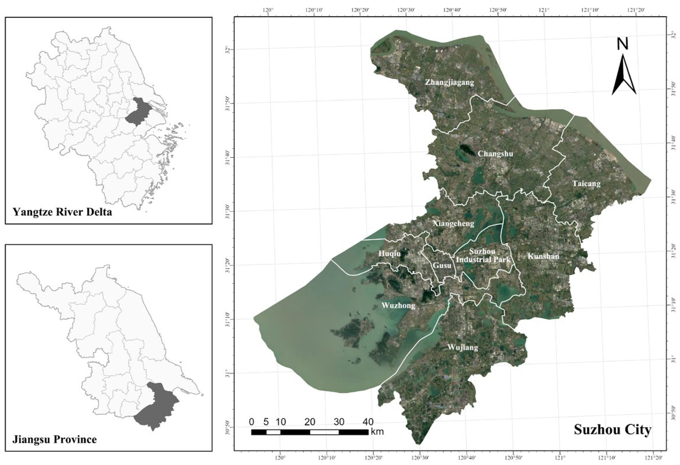
2.1. Study Area

Suzhou City is located in the southeastern part of Jiangsu Province, in the central area of the Yangtze River Delta, situated within longitudes 119°55′ to 121°20′ E and latitudes 30°47′ to 32°02′ N. It has a subtropical monsoon maritime climate characterized by warm, rainy conditions and distinct monsoon influences. In 2023, the average temperature in the urban area was 18.1 °C, with an average temperature of 6.1 °C in January and 29.7 °C in July. The total annual precipitation was 1406.8 mm, with an annual sunshine duration of 1806.3 h and an average relative humidity of 71%. The total area of Suzhou is approximately 8657.32 km², with a generally flat terrain where plains account for 54.8% of the total area, with an elevation of 3 to 4 m, gradually sloping from west to east. Rivers, lakes, and wetlands cover 34.6% of the total area, with over 20,000 rivers and more than 300 lakes, making it a typical water network city in a plain region (Figure 1).

As an important central city in the Yangtze River Delta and a renowned garden city in China, Suzhou not only has a high level of urbanization and economic development but also holds significant ecological importance in the surrounding areas. However, rapid urban expansion and changes in land use have led to ecological issues such as reduced vegetation cover, intensified heat island effects, and changes in plant phenology. Suzhou is facing an ecological crisis triggered by urbanization, making it a scientifically representative site for this study.

2.2. Data Sources

The data used in this research can mainly be divided into two categories: vegetation phenology data and land classification data. The vegetation phenology data primarily come from the MODIS land vegetation data product MOD13Q1 (MODIS/Terra Vegetation Indices 16-Day L3 Global 250 m SIN Grid), with a spatial resolution of 250 m and a temporal resolution of 16 days. Compared to other remote sensing datasets, MOD13Q1 offers excellent temporal continuity, stable vegetation indices, and an appropriate spatial resolution, making it widely utilized in studies on vegetation growth monitoring and phenological changes [19,20]. This research utilizes the NDVI layer as the data source, which has been extensively used in phenological studies of vegetation at various scales, including urban areas [21]. The study extracts the SOS, EOS, and LOS parameters from these data to characterize vegetation phenology. The land classification data refer to the LCZ classification mapping data, which are obtained using the current mainstream research method—World Urban Database and Access Portal Tools (WUDAPT) (LCZ Generator (rub.de) (https://lcz-generator.rub.de/), accessed on 1 July 2024). Multiple training simulations were conducted to ensure that the final data accuracy exceeded 80%, completing the classification mapping of the Local Climate Zones (LCZs) in Suzhou [22].

2.3. Methods

2.3.1. Extraction of Vegetation Phenological Parameters

Satellite remote sensing-based vegetation phenology research primarily analyzes the changes in vegetation indices over time to extract key time points and characteristic values [23]. Both the Normalized Difference Vegetation Index (NDVI) and the Enhanced Vegetation Index (EVI) can capture seasonal variations in vegetation characteristics and productivity. EVI is often used for monitoring the phenology of high biomass crops, while NDVI is more suitable for monitoring vegetation phenology in Suzhou, where vegetation distribution is relatively sparse [24]. First, the MOD13Q1 NDVI time series data are preprocessed to reduce the impacts of clouds, snow, aerosols, and other factors. Subsequently, data processing is conducted using software such as MATLAB R2023a and ENVI 5.6, and the Double Logistic function is employed to fit the data. The dynamic threshold method is then used to extract vegetation phenology indicators. When the maximum value and amplitude of an interval meet the threshold conditions, the increase and decrease intervals are determined as the growth period. The dates when the vegetation index rises or falls to a certain proportion are defined as the Start of the Growing Season (SOS) and End of the Growing Season (EOS), respectively. The difference between the EOS and SOS defines the Length of the Growing Season (LOS), calculated as follows [25]:

LOS = EOS − SOS

(1)

where LOS represents the length of the growing season, EOS indicates the end of the growing season, and SOS denotes the start of the growing season.

The study then cleans the data for the three key phenological indicators, removing SOS data exceeding 192 days or below 32 days, and EOS data exceeding 352 days or below 272 days. This process updates the LOS data, resulting in a more accurate dataset of key phenological periods for the study area. Finally, the trend slope S for SOS, EOS, and LOS from 2003 to 2022 is calculated using simple linear regression analysis in ArcGIS 10.8 software. The formula for the univariate linear regression equation is as follows [26]:

$$S={\displaystyle \frac{n\times \sum _{i=1}^n\left(i\times Pi\right)-\sum _{i=1}^{n}i\sum _{i=1}^n{P}_i}{n\times \sum _{i=1}^n{i}^2-{\left(\sum _{i=1}^{n}i\right)}^2}}$$

(2)

where n = 20, i is the year number, P_i is the phenological parameter for year i, and S is the slope of the univariate linear regression equation. A positive S indicates a delayed (lengthened) overall trend in phenological parameters over the 20 years, while a negative S indicates an advanced (shortened) trend.

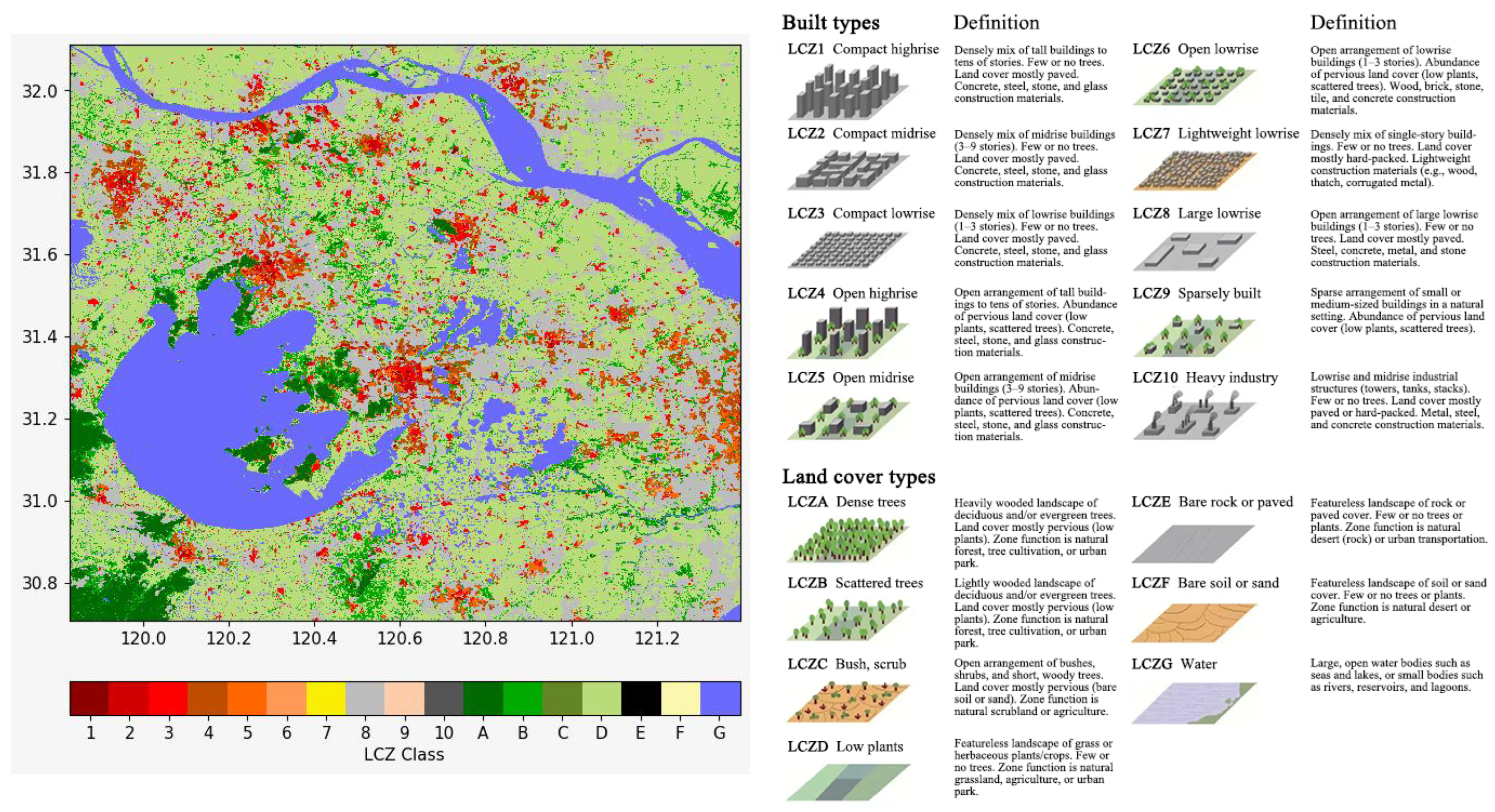
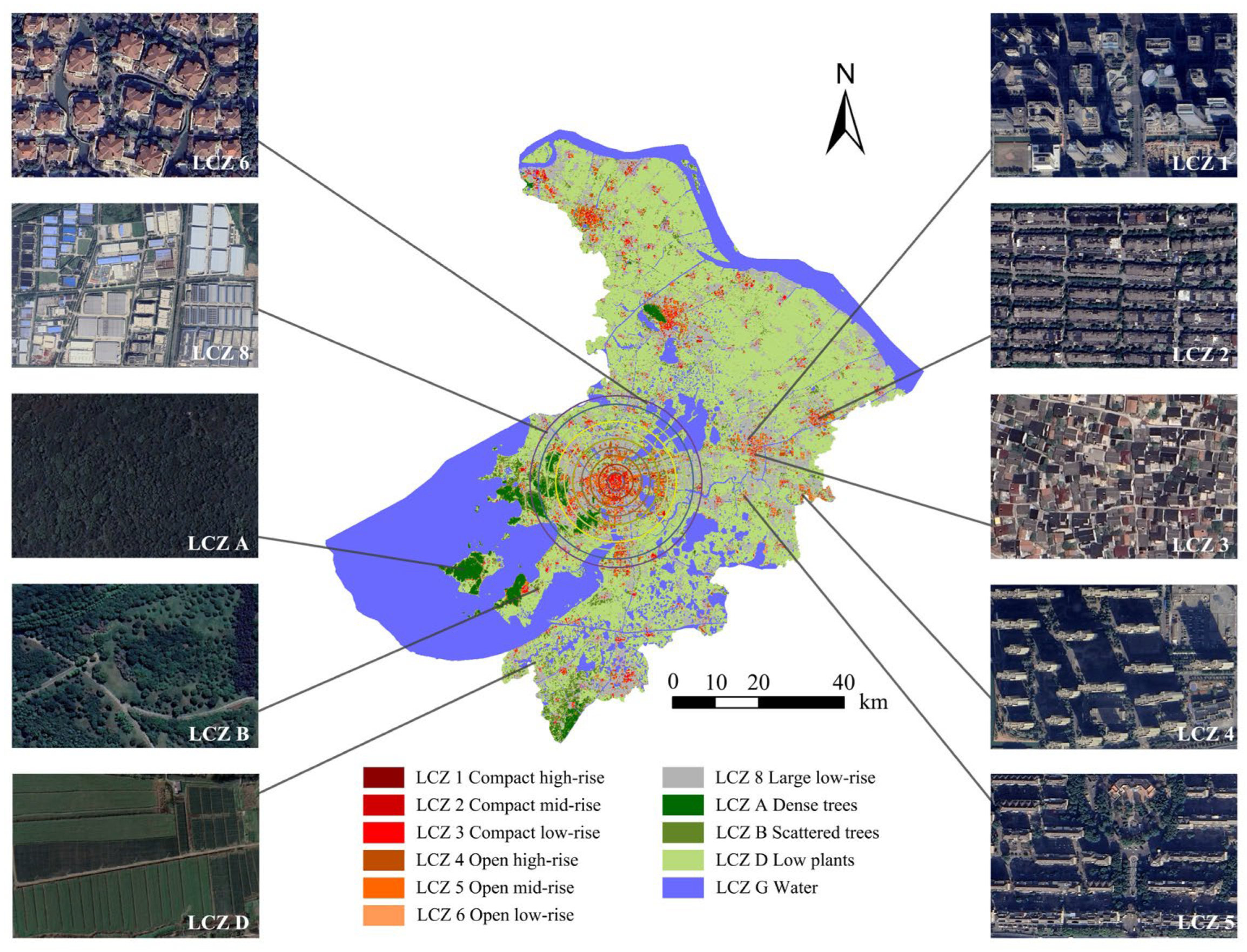
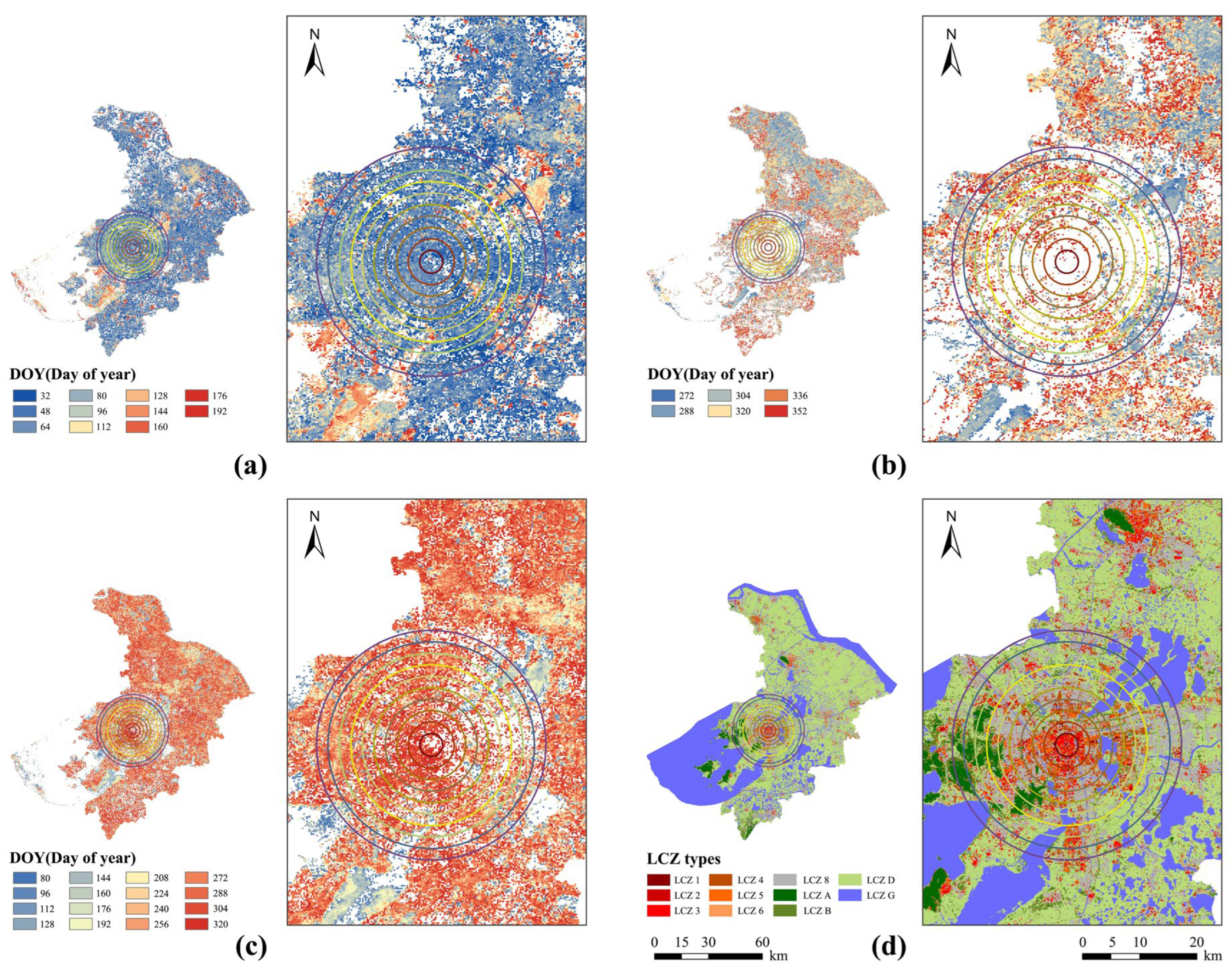
2.3.2. Mapping of Local Climate Zones (LCZs)

Among various LCZ mapping methods, those based on remote sensing imagery are widely applied, primarily including the WUDAPT method and machine learning approaches [27]. This study employs the current mainstream method—World Urban Database and Access Portal Tools (WUDAPT)—to classify the Local Climate Zones in Suzhou. First, templates for various LCZ categories used for training the model are obtained from the WUDAPT website. Based on the definitions provided by Stewart et al. for each LCZ category, the delineation of the study area’s LCZ samples is completed using Google Earth Pro 7.3.6 software [14]. The files are then uploaded to WUDAPT for model training, adjusting the delineated samples based on simulation results to improve accuracy, and repeating this process until the final model achieves an accuracy of over 80%. Finally, the simulation results are compared with historical imagery provided by Google Earth to confirm the accuracy of the land classification, completing the mapping of the Local Climate Zones in Suzhou (Figure 2).

2.3.3. Division of Urban–Rural Gradients (URGs)

In this study, the Urban–Rural Gradients (URGs) are defined by integrating Suzhou’s administrative divisions and the geometric center of the LCZ 1 parcel (compact high-rise buildings) to establish the starting point of the URGs (i.e., the urban center). Suzhou is divided into ten gradients with a radius of 2 km, resulting in categories of 2 km, 4 km, 6 km, 8 km, 10 km, 12 km, 14 km, 16 km, 18 km, and 20 km (hereinafter referred to as URG 2K, 4K, …, 18K, 20K), as shown in Figure 3.

2.3.4. Statistical Analysis of Phenological Indices Based on LCZs and URGs

The calculated phenological indicators are overlaid with the LCZs and URGs, using ArcGIS software to extract pixel values of vegetation phenology indicators for both zoning methods. These indicators are then statistically analyzed in relation to the LCZs and URGs. First, the TIFF files of SOS, EOS, and LOS from 2003 to 2022 are imported into ArcGIS software. In ArcGIS, both LCZs and URGs are converted into polygon features. The coverage tool is employed to match the phenological indicators of vegetation with the category fields of each LCZ and URG, and the merged attribute table is then exported. Subsequently, Origin and SPSS 27 are used to analyze the vegetation phenology parameters for various LCZs and URGs, and box line diagrams and line charts are created. Finally, based on the average values of SOS, EOS, and LOS for different LCZs and URGs, ANOVA is conducted to determine the differences in vegetation phenology across various LCZs and URGs. Tukey’s HSD (Honestly Significant Difference) test is used to assess the significance of differences in SOS, EOS, and LOS between the various LCZs and URGs [28], and the results are visualized using RStudio 2023.12.1. The HSD calculation formula is as follows:

$$HSD=\sqrt[q_{\alpha ,k,n-k}]{{\displaystyle \frac{MSE}{n_j}}}$$

(3)

where q is the significance level α, k is the number of means being tested, and n − k are the error degrees of freedom.

3. Results

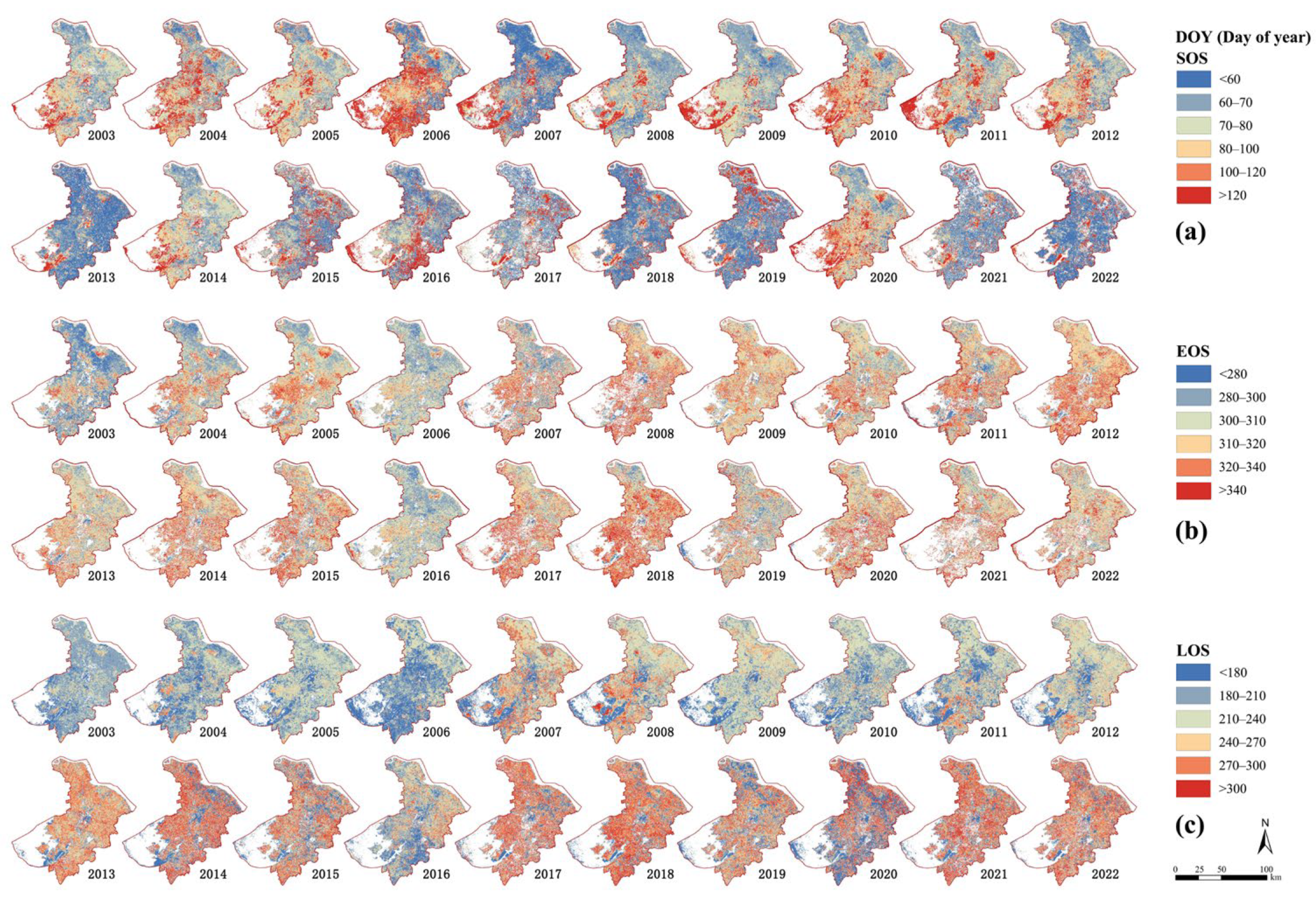
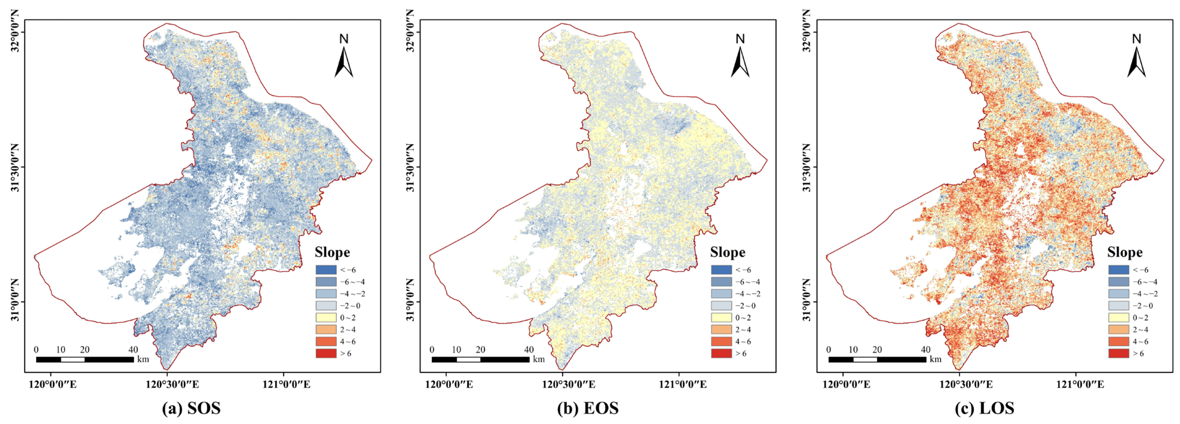
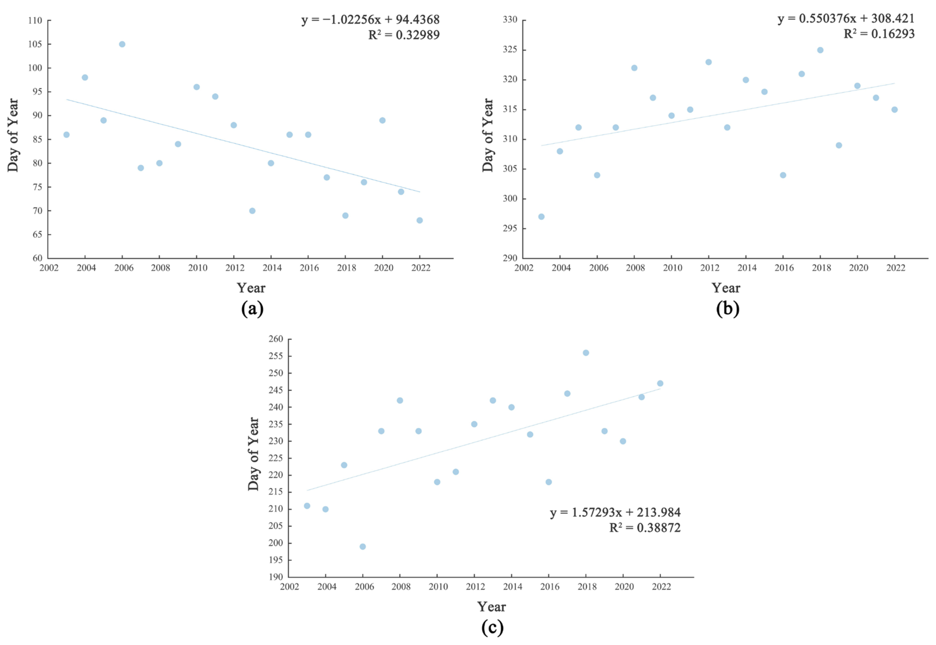
3.1. Spatio-Temporal Characteristics of Vegetation Phenology in Suzhou City

The spatial distribution map of the key phenological periods of vegetation in Suzhou from 2003 to 2022 (Figure 4) indicates that the End of the Growing Season (EOS) and Length of the Growing Season (LOS) show a significant trend of gradual advancement from the northeast to the southwest, while the Start of the Growing Season (SOS) exhibits a trend of advancement from east to west. From 2003 to 2007, the occurrence interval of EOS in the northeastern part of Suzhou primarily ranged from day 272 to day 300. However, from 2008 to 2022, the EOS in the northeast gradually delayed to the interval of day 300 to day 320. In contrast, the EOS in the central and southern regions of Suzhou mainly concentrated around day 320 to day 340, with a notable concentration even after day 340 in 2018. The latest EOS is widely distributed, mainly occurring in regions with high human activity intensity, such as the center of Zhangjiagang, Changshu, Kunshan City, and the central urban area of Suzhou. The trend of LOS is even more pronounced; from 2003 to 2006, it primarily occurred in the northeastern part of Suzhou between days 172 and 240. From 2007 to 2021, LOS was mainly concentrated between days 210 and 240. Since 2013, LOS has consistently clustered between days 270 and 300, with significant occurrences beyond day 300 in the central region in 2018 and 2021. The shortest LOS is widely distributed but predominantly found around the wetlands of lakes such as Taihu Lake, Yangcheng Lake, Kuncheng Lake, and Jinji Lake. In contrast, the spatial distribution characteristics of the longest LOS are not particularly significant. Compared to EOS and LOS, the trend of SOS changes is less pronounced, but it also shows a spatial and temporal advancement from east to west. Overall, from 2003 to 2022, SOS, EOS, and LOS exhibit widespread trends of advancement, delay, and extension, respectively.

The interannual variation trend spatial distribution map of the key phenological periods in Suzhou from 2003 to 2022 (Figure 5) shows that SOS and EOS primarily exhibit slopes of −2 to −4 and 0 to 2, respectively, under univariate linear regression analysis, while LOS shows relatively balanced positive slopes, indicating a clear hierarchical delay trend. The interannual variations in the key phenological periods also indicate (Figure 6) that during the study period, SOS, EOS, and LOS exhibit trends of advancement, delay, and extension, but the magnitude of these changes varies. Figure 6a shows that SOS advanced by an average of 1.02 days per year, with an average SOS value of 84 days, ranging from day 68 to day 105. Figure 6b indicates that EOS delayed by an average of 0.55 days per year, with an average EOS value of 314 days, fluctuating between days 297 and 325. LOS extended by an average of 1.57 days per year, with a 20-year average LOS of 231 days, ranging from day 199 to day 256 (Figure 6c).

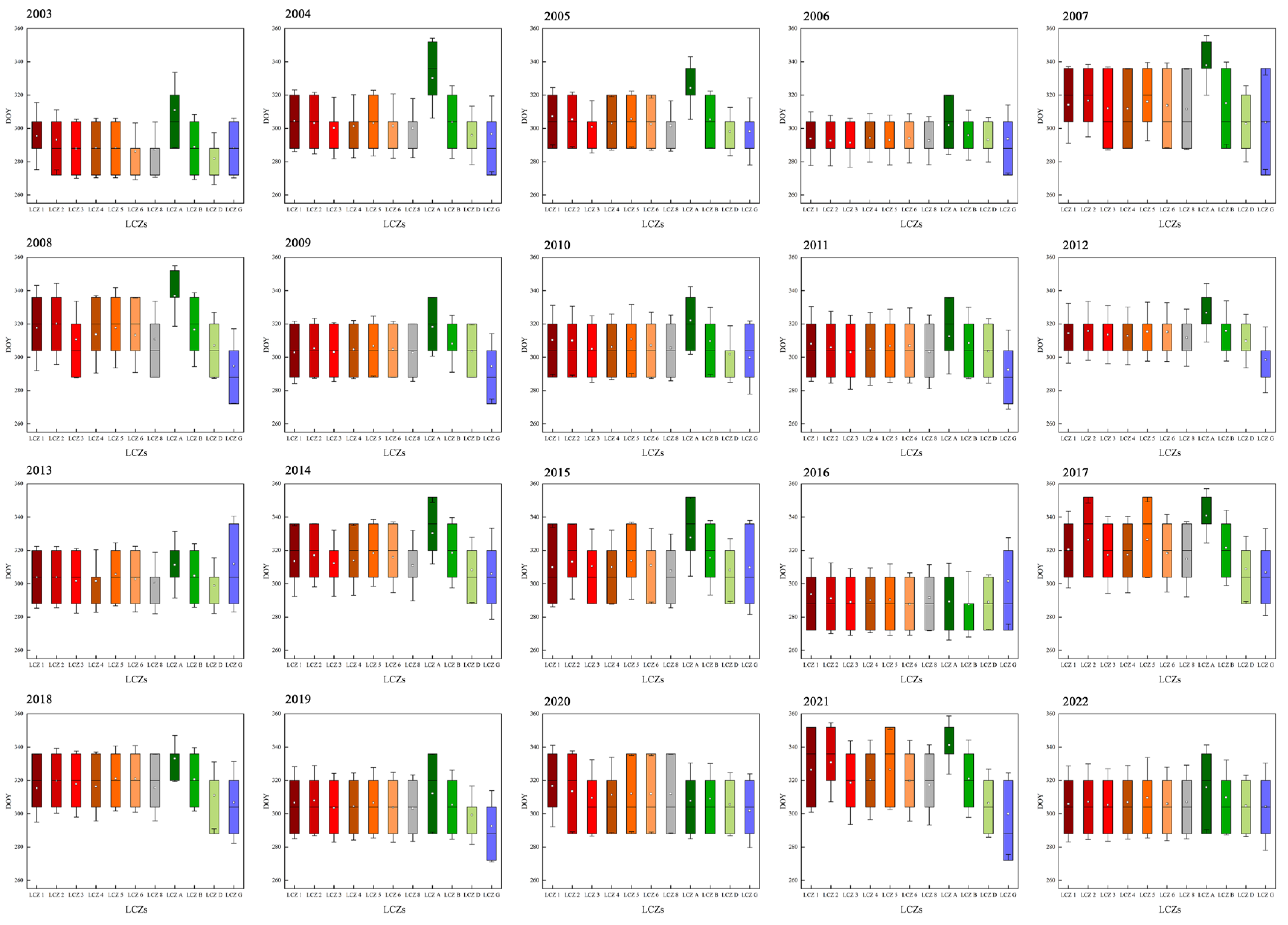
3.2. The Distribution of Vegetation Phenology of Each LCZ Category in Suzhou City

During the study period, significant differences in vegetation phenology were observed among different LCZ types, but the phenological changes between LCZ types were not significant. Relatively speaking, the EOS fluctuated widely across different LCZ categories, while the ranges for SOS and LOS were comparatively smaller (Figure 7, Figure 8 and Figure 9). The findings reveal that among the LCZ built types, LCZ 1, LCZ 2, and LCZ 5 have the most similar mean distributions. Furthermore, except for LCZ A, built types generally maintain the latest EOS, while natural land cover types, such as LCZ D and LCZ G, typically exhibit the earliest EOS. The LOS across different LCZ categories is similar to EOS, with built types usually maintaining a higher LOS than natural land cover types (except for LCZ A). Compared to EOS and LOS, built types generally have the earliest SOS (except for LCZ D), while natural land cover types LCZ G, LCZ A, and LCZ B typically exhibit the latest SOS. According to existing research, built types usually have an earlier SOS than natural land cover types, while EOS and LOS are later and longer for built types [13,25]. The earliest EOS and longest LOS observed in this study was often concentrated in the southern region of the study area, particularly in LCZ A, which may be related to the prevalence of artificial forests in the central and southern parts of Suzhou. This area is primarily dominated by artificial pure forests with simple species composition and longer overall lifecycles, leading to the phenomenon where LCZ A has greater SOS and LOS compared to built types.

In summary, built types of LCZs generally exhibit earlier SOS, later EOS, and longer LOS compared to natural land cover types. As representative areas of urban development and expansion, changes in the underlying surface and increased building density in built types contribute to rising surface and air temperatures, enhancing enzyme activity within plants, which leads to changes in plant phenology. This aligns with previous findings by Chen, Zhu, and others [29,30].

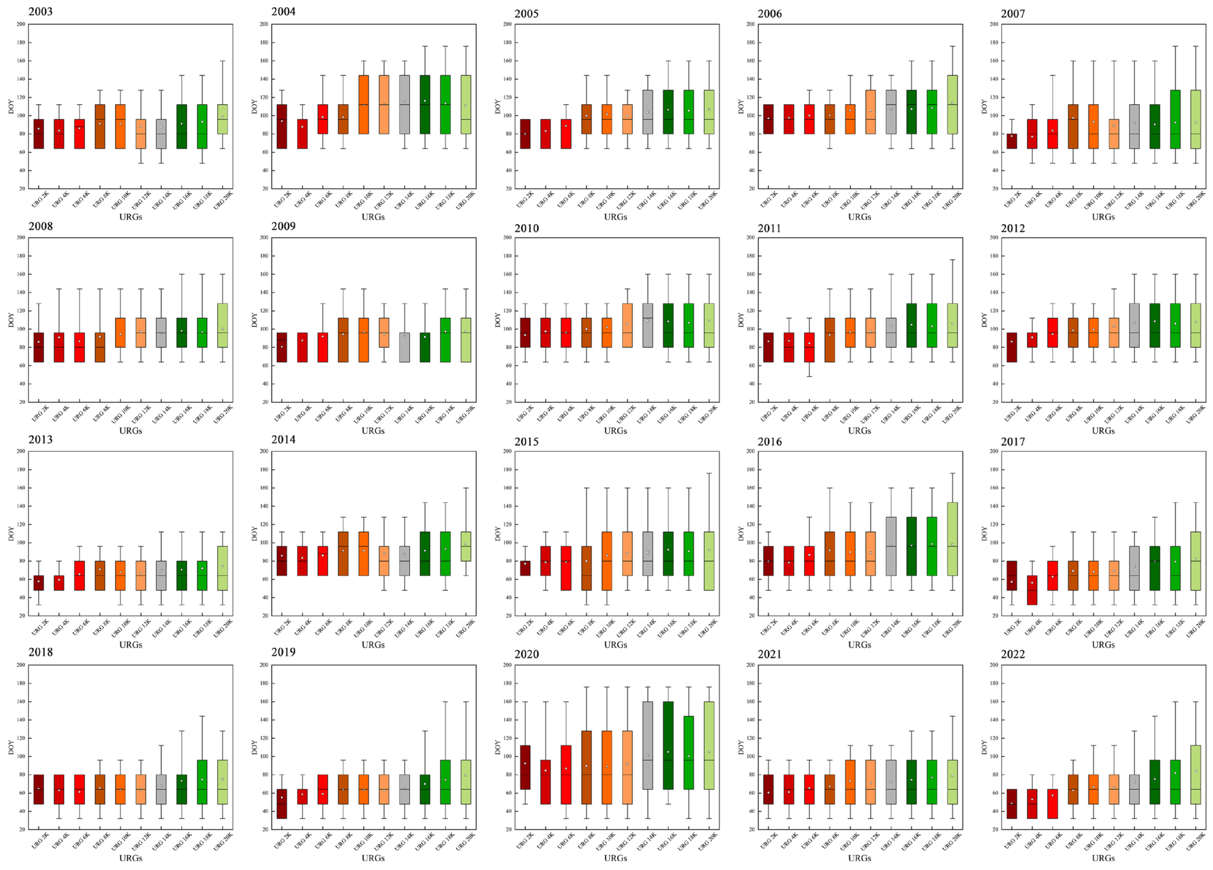
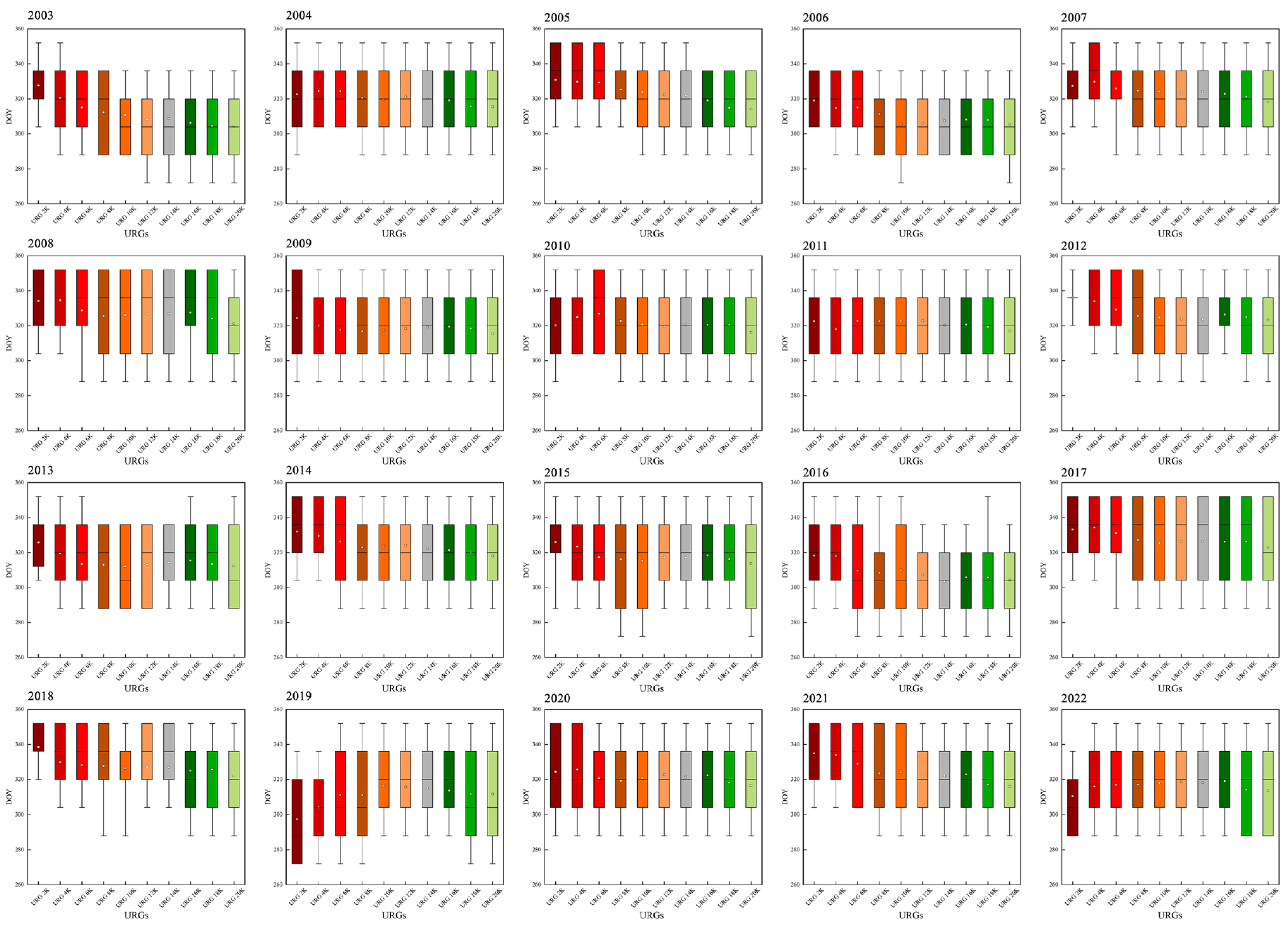
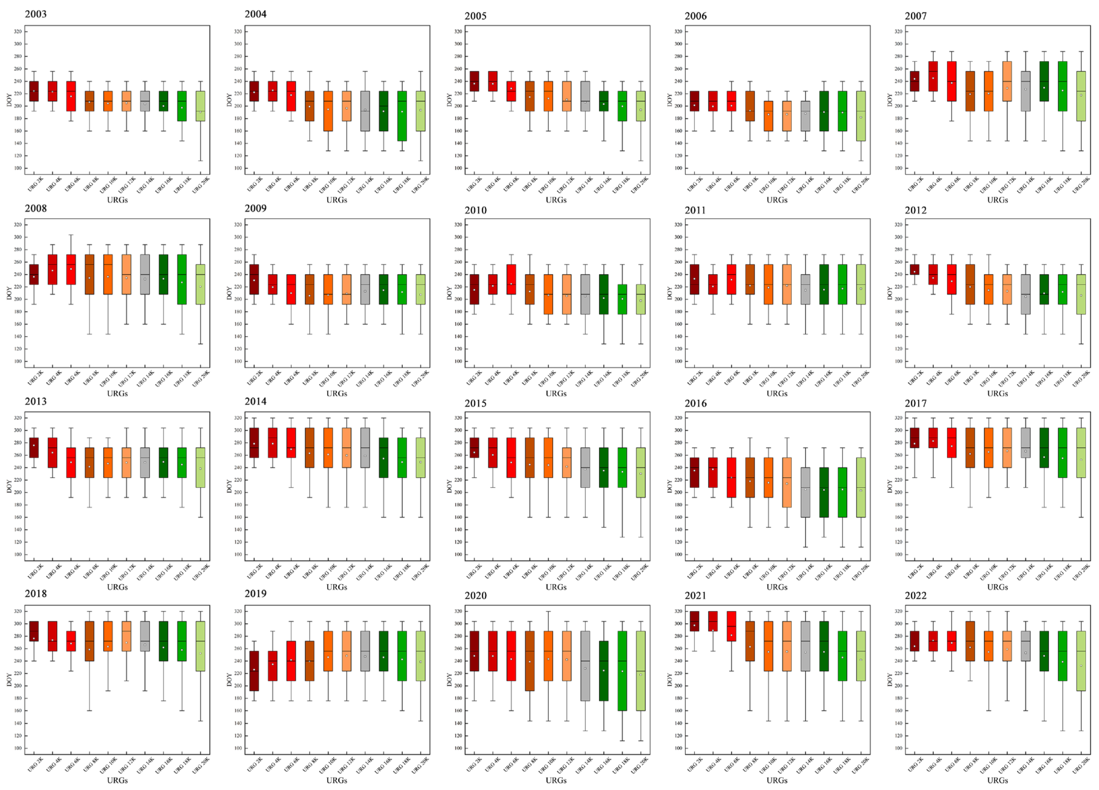
3.3. Vegetation Phenology Distribution of Each URG Category in Suzhou City

The research results indicate that the average SOS shows an overall trend of gradual delay from the urban center outward, with fluctuations between gradients generally within 30 days. The earliest average SOS typically occurs at the 2 km or 4 km gradients (Figure 10). In contrast, the average EOS exhibits an overall trend of advancement from the inner to the outer gradients, with fluctuation ranges similar to those of SOS. The latest average EOS usually appears at the 2 km or 4 km gradients, and from the 8 km gradient onward, the fluctuation range of EOS averages remains largely within 10 days, with minimal variation (Figure 11). The distribution of LOS along the Urban–Rural Gradients (URGs) is similar to that of EOS, but the average phenological parameters between gradients fluctuate comparatively more, generally ranging from 30 to 40 days (Figure 12). In summary, during the study period, as the distance from the urban center increases, SOS, EOS, and LOS exhibit trends of gradual delay, advancement, and shortening, respectively, reflecting the impact of urbanization on vegetation phenology.

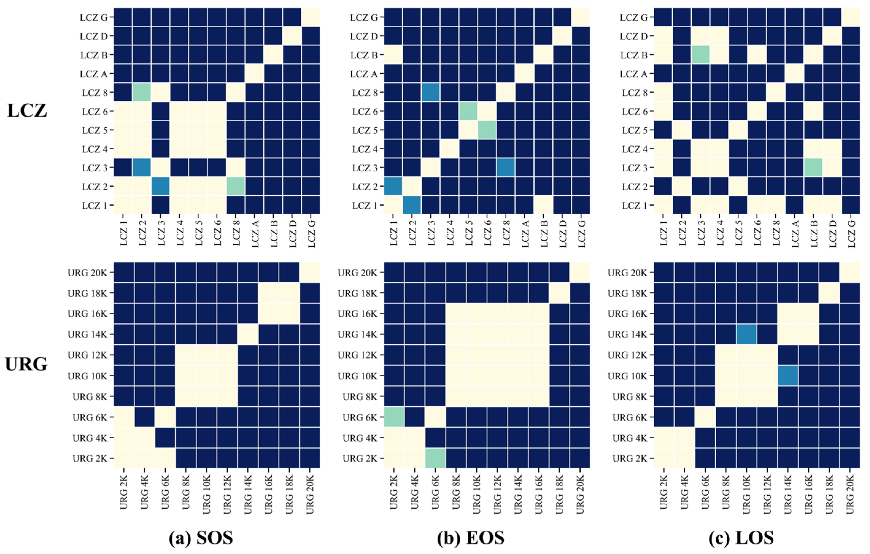
3.4. Comparative Analysis of the Key Period Parameters of Vegetation Phenology for Each URG and LCZ Category

Based on the analysis of the changes in the average parameters of the key phenological periods across various URG and LCZ categories in Suzhou over the past 20 years (Figure 13), and in conjunction with the previous study of phenological data in Suzhou, it was found that the trends in key phenological indicators across different URGs are quite pronounced. Gradients closer to the urban center exhibit earlier SOS, later EOS, and longer LOS, with these trends showing advancement, slight delay, and extension as the years progress. The changes in key phenological indicators across different LCZ categories are relatively complex. Excluding LCZ G (water bodies), which has minimal vegetation and thus influences trend analysis, and LCZ A, which has a high proportion of artificial forests and shorter growth cycles, the various LCZ categories generally demonstrate that built types (LCZ 1–10) have relatively earlier SOS, later EOS, and longer LOS compared to natural land cover types.

To further explore the differences in vegetation phenology between URG and LCZ categories, the study selected a representative year (2021) for in-depth analysis and conducted an overlay analysis of each URG and LCZ category (Figure 14). The findings reveal that the distribution ratios of built types in different Urban–Rural Gradients do not completely align with their distance from the urban center. For instance, LCZ 1 is not the most dominant built type in the URG 2K gradient (LCZ 3 is the highest), and LCZ 2 is the most prevalent in the URG 4K gradient. Additionally, LCZ 8 has the highest proportion among all LCZ types in the URG 10K gradient, resulting in a higher proportion of built types in URG 10K compared to URG 8K. The proportion of built types in LCZs gradually decreases from the urban center outward, with built types dominating within 12 km of the urban center. On the one hand, the variation in different built types between gradients is substantial, leading to significant fluctuations in phenological indicators and changes in trends (e.g., URG 8K, URG 10K). On the other hand, the proportion of natural land cover types exhibits greater variability between URG 16K and URG 20K compared to previous gradients, resulting in changes in key phenological parameters (Figure 15).

To further investigate the applicability of the two analytical methods (LCZs and URGs) in urban vegetation phenology research, the study performed one-way ANOVA and HSD tests on the average key phenological parameters of each LCZ and URG category for 2021 (Figure 16). The results indicate that the significant logarithms of LCZ for SOS, EOS, and LOS are 44, 54, and 43, respectively, with significant difference proportions of 66.7%, 81.8%, and 65.2%. In contrast, the significant logarithms of URG are 39, 34, and 40, with difference proportions of 70.9%, 61.8%, and 72.7%. The ratio of significant differences for SOS and LOS among the various LCZ and URG pairs is relatively consistent; however, the proportion of significant differences for EOS in LCZ pairs is notably higher than that in URG pairs, indicating greater statistical significance. Overall, the vegetation phenological differences among various LCZ types are more pronounced and statistically significant compared to URG pairs.

4. Discussion

4.1. Local Climate Zones and Urban–Rural Gradients

Urban vegetation phenology often varies with different levels of urbanization, geographical locations, and heat island intensity, and is influenced by multiple factors and characterized by complex mechanisms. Urban–Rural Gradients (URGs) facilitate spatial analysis of vegetation phenology changes by establishing the urban center and examining differences in horizontal distances. According to the results of this study, urban vegetation phenology exhibits a trend of gradually delayed SOS, advanced EOS, and shortened LOS as one moves outward from the urban center. This reflects the impact of urbanization on vegetation phenology and aligns with existing research on interannual variations in vegetation phenology. However, the consideration of spatial changes in urban vegetation phenology through URGs is relatively simplistic, as it analyzes solely from a two-dimensional distance perspective without incorporating relevant indicators that reflect the complexity of urban ecosystems, such as underlying surface conditions, building characteristics, slope, and aspect. This limitation may hinder the advancement of more detailed urban vegetation phenology studies.

In contrast to Urban–Rural Gradients (URGs), Local Climate Zones (LCZs) incorporate the three-dimensional structural characteristics of buildings into land use classification, using indicators such as building height and density to describe the urban canopy. This approach standardizes urban morphology and functional zoning, providing a more comprehensive reflection of the complexity of the environment in which urban vegetation exists, thereby offering a better theoretical framework for phenological studies. The results of this study indicate that analyses of key phenological periods based on LCZs show that built types generally exhibit earlier SOS, later EOS, and longer LOS compared to natural cover types. This is consistent with the results of phenological changes from the urban center to suburban areas observed in URG analyses. However, the spatial distribution of built types in LCZs is not concentric, like that defined by URGs, and their proportions do not change progressively with increasing distance from the urban center. This reflects the non-concentrated distribution of built types in the study area and the complex characteristics of the research environment, which also influence the temporal and spatial trends in vegetation phenology. The changes in EOS begin to stabilize from the 8 km distance from the urban center (URG 8K) as the gradient increases, which may correlate with the stabilization of built type proportions in LCZs. The higher proportion and greater fluctuation of built types in URG 2K and URG 4K often maintain the earliest SOS and the latest EOS. This is likely due to the impermeable nature of built types, leading to higher surface temperatures compared to natural cover types. Because air temperatures in urban canopies are significantly influenced by building form, materials, underlying surface conditions, and anthropogenic heat, these areas experience higher air temperatures. Coupled with the high sensible heat flux characteristic of large built-up areas, this exacerbates the urban heat island (UHI) phenomenon. Given that spring phenology in vegetation is primarily regulated by temperature, rising temperatures can lead to significantly earlier spring growth. Increased temperatures can also affect autumn phenology, resulting in delayed EOS and thus extending LOS. This finding is consistent with the results of this study and aligns with observed phenological change patterns in regions such as Africa [31], the southern United States [28], many cities in China [32], and other mid- to high-latitude areas in the Northern Hemisphere [33,34]. In summary, compared to the partitioning method of URGs, the LCZ classification method, which comprehensively considers urban underlying surface conditions and three-dimensional structures, is evidently more scientifically sound. Combined with the results of the HSD test analysis in this study, LCZs are not only applicable to current research on urban ecosystems’ responses to urban heat islands but also well-suited for future complex studies of urban vegetation phenology.

4.2. Analysis of Spatial and Temporal Characteristics of Urban Vegetation Phenology

The temporal and spatial changes in urban vegetation phenology are closely related to urbanization. The results indicate that with increasing levels of urbanization, urban vegetation phenology tends to show earlier Start of the Growing Season (SOS), delayed End of the Growing Season (EOS), and extended Length of the Growing Season (LOS). However, the specific impacts of urbanization on changes in vegetation phenology are multifactorial and involve complex mechanisms. For instance, increased carbon dioxide concentrations can lead to earlier SOS and delayed EOS, while changes in underlying surfaces can result in increased surface accumulation temperatures and air temperatures, contributing to extended LOS. Factors such as photoperiod, hydrological conditions, topography, species, and human activities also influence changes in urban vegetation phenology. In this study, the phenology of artificial forests (LCZ A) and cropland (LCZ D), affected by human activities and species types, exhibited differences from other areas, introducing some uncertainty into the research results. Future studies should explore in depth the driving mechanisms of various factors affecting vegetation phenology changes in the context of urbanization.

The analysis of the spatiotemporal distribution characteristics of vegetation phenology typically employs satellite remote sensing methods to extract phenological parameters. The choice of remote sensing datasets and extraction methods may introduce some uncertainties into the experimental results. The MOD13Q1 dataset used in this study has a high temporal resolution but relatively low spatial resolution. Due to the influence of meteorological factors and cloud cover, the data may contain outliers and missing values, which may hinder the ability to capture finer-scale urban vegetation characteristics and variations in vegetation changes. To address the outliers in the phenological data, this study applied a threshold method based on existing research results and field observations, removing SOS data older than the 192nd day or younger than the 32nd day, as well as EOS data older than the 352nd day or younger than the 272nd day, and subsequently updating the LOS data. After cleaning the outliers, some areas with missing values appeared on the maps, primarily around water bodies, which did not significantly affect the analysis of temporal and spatial changes in vegetation phenology. According to the results of this study, the overall trend of vegetation phenology in Suzhou shows earlier SOS, delayed EOS, and extended LOS, which is consistent with previous research on temporal changes in vegetation phenology. The cleaning of outliers did not lead to significant deviations in the research results. To address the issue of low data resolution preventing the extraction of detailed vegetation indicators, it is advisable to select appropriate high-resolution remote sensing products or employ emerging technologies for the data fusion of remote sensing data to obtain more accurate and detailed vegetation phenology information. For instance, using high-resolution multispectral satellite data such as Landsat to extract urban vegetation phenology indicators [7], or utilizing remote sensing-based solar-induced chlorophyll fluorescence (SIF) data for phenological research, could replace the commonly used methods based on NDVI data for extracting key phenological parameters [35,36]. With the continuous evolution of new satellite remote sensing data and analytical techniques, there are increasing opportunities for a deeper exploration of the complex mechanisms underlying temporal and spatial changes in urban vegetation phenology.

5. Conclusions

This study extracted the key period parameters SOS, EOS, and LOS of vegetation phenology in Suzhou from 2003 to 2022 using the MOD13Q1 dataset, and linked these parameters to Local Climate Zones (LCZs) and Urban–Rural Gradients (URGs) to explore the temporal and spatial distribution characteristics of urban vegetation phenology in Suzhou. The research validated the impact of urbanization on urban vegetation phenology and provided a basis for optimizing urban plant maintenance management, climate regulation, and the quality of the human living environment, thereby contributing to the construction and development of sustainable cities.

The results revealed that during the study period, the average SOS in Suzhou advanced by 1.02 days per year, the average EOS was delayed by 0.55 days per year, and the average LOS extended by 1.57 days per year. Overall, built types in LCZs exhibited earlier SOS, later EOS, and longer LOS compared to natural land cover types. As the URG gradient progresses outward from the city center, vegetation phenology shows a trend of gradually delayed SOS, gradually advanced EOS, and gradually shortened LOS. Moreover, the differences in vegetation phenology within LCZ pairs are more pronounced and statistically significant than those within URG pairs. The study found that LCZs account for the complexity of urban ecosystems by incorporating three-dimensional information, such as buildings and underlying surfaces, into land use classification. This approach is more aligned with the characteristics of temporal and spatial changes in urban vegetation phenology than the simpler two-dimensional perspective of URGs, which considers only the distance from the urban center. This provides a novel perspective for future explorations of the mechanisms behind urban vegetation phenology changes and the interactions between urbanization, climate change, and vegetation phenology. Future research holds potential for further exploration and optimization of LCZs by enhancing their alignment with studies on vegetation phenology under various contexts such as urbanization and climate change, thereby maximizing their advantages and value. Additionally, investigating how to construct multidimensional and comprehensive urban vegetation research models is another valuable and meaningful direction for future studies. For instance, combining LCZs with URGs or other methodologies to develop analytical and evaluation models for urban vegetation phenology, as well as integrating phenological data with climate change prediction models to create forecasts of changes in urban vegetation phenology, represent areas that warrant further investigation by researchers.

References

1. Piao, S.; Liu, Q.; Chen, A.; Janssens, I.A.; Fu, Y.; Dai, J.; Liu, L.; Lian, X.; Shen, M.; Zhu, X. Plant phenology and global climate change: Current progresses and challenges. Glob. Change Biol. 2019, 25, 1922–1940. [Google Scholar] [CrossRef]
2. Zhang, L.; Yang, L.; Zohner, C.M.; Crowther, T.W.; Li, M.; Shen, F.; Guo, M.; Qin, J.; Yao, L.; Zhou, C. Direct and indirect impacts of urbanization on vegetation growth across the world’s cities. Sci. Adv. 2022, 8, eabo0095. [Google Scholar] [CrossRef]
3. Li, L.; Li, X.; Asrar, G.; Zhou, Y.; Chen, M.; Zeng, Y.; Li, X.; Li, F.; Luo, M.; Sapkota, A. Detection and attribution of long-term and fine-scale changes in spring phenology over urban areas: A case study in New York State. Int. J. Appl. Earth Obs. Geoinf. 2022, 110, 102815. [Google Scholar]
4. Su, Y.; Liu, L.; Liao, J.; Wu, J.; Ciais, P.; Liao, J.; He, X.; Liu, X.; Chen, X.; Yuan, W. Phenology acts as a primary control of urban vegetation cooling and warming: A synthetic analysis of global site observations. Agric. For. Meteorol. 2020, 280, 107765. [Google Scholar]
5. Zeng, Y.; Hao, D.; Huete, A.; Dechant, B.; Berry, J.; Chen, J.M.; Joiner, J.; Frankenberg, C.; Bond-Lamberty, B.; Ryu, Y. Optical vegetation indices for monitoring terrestrial ecosystems globally. Nat. Rev. Earth Environ. 2022, 3, 477–493. [Google Scholar] [CrossRef]
6. Hassan, T.; Gulzar, R.; Hamid, M.; Ahmad, R.; Waza, S.A.; Khuroo, A.A. Plant phenology shifts under climate warming: A systematic review of recent scientific literature. Environ. Monit. Assess. 2024, 196, 36. [Google Scholar] [CrossRef]
7. Zeng, L.; Wardlow, B.D.; Xiang, D.; Hu, S.; Li, D. A review of vegetation phenological metrics extraction using time-series, multispectral satellite data. Remote Sens. Environ. 2020, 237, 111511. [Google Scholar]
8. Gong, Z.; Ge, W.; Guo, J.; Liu, J. Satellite remote sensing of vegetation phenology: Progress, challenges, and opportunities. ISPRS J. Photogramm. Remote Sens. 2024, 217, 149–164. [Google Scholar]
9. Yang, L.; Zhao, S.; Liu, S. Urban environments provide new perspectives for forecasting vegetation phenology responses under climate warming. Glob. Change Biol. 2023, 29, 4383–4396. [Google Scholar]
10. Wang, L.; De Boeck, H.J.; Chen, L.; Song, C.; Chen, Z.; McNulty, S.; Zhang, Z. Urban warming increases the temperature sensitivity of spring vegetation phenology at 292 cities across China. Sci. Total Environ. 2022, 834, 155154. [Google Scholar]
11. Yang, C.; Wu, H.; Xie, C.; Wan, Y.; Qin, Y.; Jiang, R.; Zhang, Y.; Che, S. Community future climate resilience assessment based on CMIP6, A case study of communities along an urban-rural gradient in Shanghai. Urban Clim. 2024, 56, 101966. [Google Scholar] [CrossRef]
12. Yang, J.; Luo, X.; Jin, C.; Xiao, X.; Xia, J.C. Spatiotemporal patterns of vegetation phenology along the urban–rural gradient in Coastal Dalian, China. Urban For. Urban Green. 2020, 54, 126784. [Google Scholar] [CrossRef]
13. Xie, J.; Li, X.; Chung, L.C.H.; Webster, C.J. Effects of land surface temperatures on vegetation phenology along urban–rural local climate zone gradients. Landsc. Ecol. 2024, 39, 62. [Google Scholar] [CrossRef]
14. Stewart, I.D.; Oke, T.R. Local climate zones for urban temperature studies. Bull. Am. Meteorol. Soc. 2012, 93, 1879–1900. [Google Scholar] [CrossRef]
15. Demuzere, M.; Kittner, J.; Martilli, A.; Mills, G.; Moede, C.; Stewart, I.D.; Van Vliet, J.; Bechtel, B. A global map of Local Climate Zones to support earth system modelling and urban scale environmental science. Earth Syst. Sci. Data Discuss. 2022, 2022, 3835–3873. [Google Scholar] [CrossRef]
16. Xia, H.; Chen, Y.; Song, C.; Li, J.; Quan, J.; Zhou, G. Analysis of surface urban heat islands based on local climate zones via spatiotemporally enhanced land surface temperature. Remote Sens. Environ. 2022, 273, 112972. [Google Scholar] [CrossRef]
17. Du, S.; Zhang, X.; Jin, X.; Zhou, X.; Shi, X. A review of multi-scale modelling, assessment, and improvement methods of the urban thermal and wind environment. Build. Environ. 2022, 213, 108860. [Google Scholar] [CrossRef]
18. Aslam, A.; Rana, I.A. The use of local climate zones in the urban environment: A systematic review of data sources, methods, and themes. Urban Clim. 2022, 42, 101120. [Google Scholar] [CrossRef]
19. Ahmed, T.; Singh, D. Probability density functions based classification of MODIS NDVI time series data and monitoring of vegetation growth cycle. Adv. Space Res. 2020, 66, 873–886. [Google Scholar] [CrossRef]
20. Cai, Z.; Jönsson, P.; Jin, H.; Eklundh, L. Performance of smoothing methods for reconstructing NDVI time-series and estimating vegetation phenology from MODIS data. Remote Sens. 2017, 9, 1271. [Google Scholar] [CrossRef]
21. Wu, Y.; Tang, G.; Gu, H.; Liu, Y.; Yang, M.; Sun, L. The variation of vegetation greenness and underlying mechanisms in Guangdong province of China during 2001–2013 based on MODIS data. Sci. Total Environ. 2019, 653, 536–546. [Google Scholar] [PubMed]
22. Wang, R.; Wang, M.; Ren, C.; Chen, G.; Mills, G.; Ching, J. Mapping local climate zones and its applications at the global scale: A systematic review of the last decade of progress and trend. Urban Clim. 2024, 57, 102129. [Google Scholar]
23. Ferchichi, A.; Abbes, A.B.; Barra, V.; Farah, I.R. Forecasting vegetation indices from spatio-temporal remotely sensed data using deep learning-based approaches: A systematic literature review. Ecol. Inform. 2022, 68, 101552. [Google Scholar]
24. Lv, J.; Zhao, W.; Hua, T.; Zhang, L.; Pereira, P. Multiple Greenness Indexes revealed the vegetation greening during the growing season and winter on the Tibetan Plateau despite regional variations. Remote Sens. 2023, 15, 5697. [Google Scholar] [CrossRef]
25. Li, S.; Li, Q.; Zhang, J.; Zhang, S.; Wang, X.; Yang, S.; Zhang, S. Study on the Spatial and Temporal Distribution of Urban Vegetation Phenology by Local Climate Zone and Urban–Rural Gradient Approach. Remote Sens. 2023, 15, 3957. [Google Scholar] [CrossRef]
26. Liu, N.; Shi, Y.; Ding, Y.; Liu, L.; Peng, S. Temporal effects of climatic factors on vegetation phenology on the Loess Plateau, China. J. Plant Ecol. 2023, 16, rtac063. [Google Scholar]
27. Huang, F.; Jiang, S.; Zhan, W.; Bechtel, B.; Liu, Z.; Demuzere, M.; Huang, Y.; Xu, Y.; Ma, L.; Xia, W. Mapping local climate zones for cities: A large review. Remote Sens. Environ. 2023, 292, 113573. [Google Scholar]
28. Zhao, C.; Weng, Q.; Wang, Y.; Hu, Z.; Wu, C. Use of local climate zones to assess the spatiotemporal variations of urban vegetation phenology in Austin, Texas, USA. GIScience Remote Sens. 2022, 59, 393–409. [Google Scholar]
29. Chen, Y.; Lin, M.; Lin, T.; Zhang, J.; Jones, L.; Yao, X.; Geng, H.; Liu, Y.; Zhang, G.; Cao, X. Spatial heterogeneity of vegetation phenology caused by urbanization in China based on remote sensing. Ecol. Indic. 2023, 153, 110448. [Google Scholar]
30. Zhu, E.; Fang, D.; Chen, L.; Qu, Y.; Liu, T. The Impact of Urbanization on Spatial–Temporal Variation in Vegetation Phenology: A Case Study of the Yangtze River Delta, China. Remote Sens. 2024, 16, 914. [Google Scholar] [CrossRef]
31. Shi, S.; Yang, P.; van der Tol, C. Spatial-temporal dynamics of land surface phenology over Africa for the period of 1982–2015. Heliyon 2023, 9, e16413. [Google Scholar] [CrossRef] [PubMed]
32. Hu, M.; Li, X.; Xu, Y.; Huang, Z.; Chen, C.; Chen, J.; Du, H. Remote sensing monitoring of the spatiotemporal dynamics of urban forest phenology and its response to climate and urbanization. Urban Clim. 2024, 53, 101810. [Google Scholar] [CrossRef]
33. Wu, F.; Jiang, Y.; Wen, Y.; Zhao, S.; Xu, H. Spatial synchrony in the start and end of the thermal growing season has different trends in the mid-high latitudes of the Northern Hemisphere. Environ. Res. Lett. 2021, 16, 124017. [Google Scholar] [CrossRef]
34. Yin, H.; Liu, Q.; Liao, X.; Ye, H.; Li, Y.; Ma, X. Refined Analysis of Vegetation Phenology Changes and Driving Forces in High Latitude Altitude Regions of the Northern Hemisphere: Insights from High Temporal Resolution MODIS Products. Remote Sens. 2024, 16, 1744. [Google Scholar] [CrossRef]
35. Zheng, C.; Wang, S.; Chen, J.M.; Chen, J.; Chen, B.; He, X.; Li, H.; Sun, L. Combination of vegetation indices and SIF can better track phenological metrics and gross primary production. J. Geophys. Res. Biogeosci. 2023, 128, e2022JG007315. [Google Scholar] [CrossRef]
36. Zhang, J.; Gonsamo, A.; Tong, X.; Xiao, J.; Rogers, C.A.; Qin, S.; Liu, P.; Yu, P.; Ma, P. Solar-induced chlorophyll fluorescence captures photosynthetic phenology better than traditional vegetation indices. ISPRS J. Photogramm. Remote Sens. 2023, 203, 183–198. [Google Scholar] [CrossRef]
Figure 1. Location and satellite map of the study area.
Sustainability 17 02970 g001
Figure 2. The mapping results of Local Climate Zones (LCZs) in the study area and the illustration and definition of each LCZ category.
Sustainability 17 02970 g002
Figure 3. The spatial distribution of LCZs and the division of Urban–Rural Gradients of Suzhou.
Sustainability 17 02970 g003
Figure 4. Spatial distributions of (a) SOS, (b) EOS, and (c) LOS in Suzhou from 2003 to 2022.
Sustainability 17 02970 g004
Figure 5. Spatial distributions of interannual variation trends of (a) SOS, (b) EOS, and (c) LOS in Suzhou from 2003 to 2022.
Sustainability 17 02970 g005
Figure 6. The interannual variability of (a) SOS, (b) EOS, and (c) LOS in Suzhou from 2003 to 2022. Note: The blue dot corresponds to the average value of the phenological index of a year, and the blue line represents the linear regression line of these points.
Sustainability 17 02970 g006
Figure 7. The box line diagram of SOS distribution of different LCZ categories in Suzhou from 2003 to 2022. Note: The whisker range of the box plot is 1 times the standard deviation of the coefficient (Standard Deviation, SD).
Sustainability 17 02970 g007
Figure 8. The box line diagram of EOS distribution of different LCZ categories in Suzhou from 2003 to 2022.
Sustainability 17 02970 g008
Figure 9. The box line diagram of LOS distribution of different LCZ categories in Suzhou from 2003 to 2022.
Sustainability 17 02970 g009
Figure 10. The box line diagram of SOS distribution of different URG categories in Suzhou from 2003 to 2022.
Sustainability 17 02970 g010
Figure 11. The box line diagram of EOS distribution of different URG categories in Suzhou from 2003 to 2022.
Sustainability 17 02970 g011
Figure 12. The box line diagram of LOS distribution of different URG categories in Suzhou from 2003 to 2022.
Sustainability 17 02970 g012
Figure 13. The variation trend of the mean values of LCZ and URG categories: (a) SOS, (b) EOS, and (c) LOS in Suzhou from 2003 to 2022.
Sustainability 17 02970 g013
Figure 14. The (a) SOS, (b) EOS, and (c) LOS distribution on URGs in 2021 and (d) LCZs along URGs in 2021.
Sustainability 17 02970 g014
Figure 15. The average change in phenological critical period of each URG category and the proportion of each LCZ type on each gradient in 2021.
Sustainability 17 02970 g015
Figure 16. HSD test results of (a) SOS, (b) EOS, and (c) LOS based on LCZ and URG in 2021. Note: Yellow indicates no significant difference, dark blue, blue, and green indicate significant difference, and the significance levels were 0.001, 0.01 and 0.05, respectively.
Sustainability 17 02970 g016
Disclaimer/Publisher’s Note: The statements, opinions and data contained in all publications are solely those of the individual author(s) and contributor(s) and not of MDPI and/or the editor(s). MDPI and/or the editor(s) disclaim responsibility for any injury to people or property resulting from any ideas, methods, instructions or products referred to in the content.