Enhanced TSMixer Model for the Prediction and Control of Particulate Matter

Abstract

This study presents an improved deep-learning model, termed Enhanced Time Series Mixer (E-TSMixer), for the prediction of particulate matter. By analyzing the temporal evolution of PM_2.5 concentrations from multivariate monitoring data, the model demonstrates significant prediction capabilities while maintaining consistency with observed pollutant transport characteristics in the urban boundary layer. In E-TSMixer, a fully connected output layer is proposed to enhance the predictive capability for complex spatiotemporal dependencies. The relevant data on air quality and traffic flow are fused to achieve high-precision predictions of PM_2.5 concentrations through a multivariate time-series forecasting model. An asymmetric penalty mechanism is added to dynamically optimize the loss function. Experimental results indicate that the proposed E-TSMixer model achieves higher accuracy for the prediction of PM_2.5, which significantly outperforms the traditional models. Additionally, an intelligent dual regulation of fixed and dynamic threshold model is introduced and combined with E-TSMixer for the decision-making model of the real-time adjustments of the frequency, routes, and timing of water truck operation in practice.

1. Introduction

With the acceleration of urbanization, activities such as construction projects, road works, and transportation have increased in frequency, exacerbating the issue of road dust particulate pollution. Road dust particles, particularly PM_2.5 and PM₁₀, not only significantly deteriorate urban air quality but also pose a major threat to the respiratory and cardiovascular health of residents. Studies indicated that long-term exposure to high concentrations of particulate matter can lead to various chronic diseases, including asthma, bronchitis, and heart disease [1]. Furthermore, road dust pollution adversely affects the aesthetic quality of urban environments, diminishing their livability [2]. Therefore, effectively controlling road dust emissions and mitigating their impact on air quality has become a pressing issue in urban environmental management.

Effective prediction and detection of PM_2.5 concentrations exceeding regulatory thresholds is a critical requirement in the context of air quality management, particularly in regions where stringent air pollution regulations are enforced. Instances of pollutant concentrations surpassing these thresholds often trigger extensive regulatory interventions, including temporary shutdowns of industrial activities, restrictions on transportation, and heightened enforcement of emission controls. These measures, while necessary, impose substantial socioeconomic costs, making it imperative to accurately capture and predict threshold-exceeding events to enable timely and targeted responses. Exceeding regulatory thresholds for PM_2.5 concentrations is unacceptable from a governance perspective due to its potential to compromise public health and trigger widespread regulatory actions. For policymakers, accurate early warnings of threshold breaches are indispensable, as they provide the basis for implementing preemptive measures and mitigating the escalation of pollution events. The frequency and accuracy of such threshold-exceedance predictions, therefore, play a pivotal role in supporting government decision-making processes. Moreover, the ability to capture and respond to these critical events not only ensures compliance with regulatory frameworks but also aligns with broader goals of environmental sustainability and public health protection. This underlines the necessity of developing predictive models that prioritize the detection of threshold-exceeding pollution levels over marginal improvements in overall statistical accuracy.

Traditional road dust control methods typically rely on water trucks [3]. While these methods can reduce road dust concentrations to some extent, most road dust suppression operations depend on manual inspections and fixed-frequency applications, lacking precise real-time air quality perception and dynamic adjustment capabilities. This often results in delayed responses and limited coverage. For example, during traffic congestion or peak construction periods, fluctuations in particulate concentrations can be significant; fixed-frequency water truck operations may yield suboptimal road dust suppression results and even lead to resource wastage [4]. Traditional approaches are inflexible in adapting to these variable conditions and lack intelligent responses to changes in weather conditions and traffic flow.

Recently, the advancements in the Internet of Things (IoT), big data, and artificial intelligence have accelerated the intelligent transformation of urban environmental governance [5,6]. Big data-driven predictive technologies offer new directions for air pollution prevention and control. By leveraging real-time monitoring and deep-learning models, air quality trends can be forecasted, enabling more scientific and efficient road dust control decision-making. Against this backdrop, a district in Guangdong Province has begun to deploy air quality monitoring systems, traffic flow monitoring systems, and big data analytics platforms, achieving precise monitoring of air quality and particulate concentrations. However, the key challenge remains how to effectively integrate these data sources to construct an intelligent road dust control system.

To address these challenges, this study presents an improved deep-learning model, termed Enhanced TSMixer (E-TSMixer), for the intelligent prediction and control of PM_2.5. The model integrates air quality and traffic flow data to provide high-precision predictions of particulate matter concentrations. This approach incorporates mechanisms to enhance its reliability in detecting and predicting concentration peaks over regulatory limits, optimizing both environmental outcomes and resource utilization. While utilizing data collected from Shenzhen, China, the core framework of E-TSMixer is based on universal mathematical and algorithmic principles, making it inherently adaptable to various environmental contexts with appropriate parameter adjustments.

The contributions of this work are summarized in three folds.

(1)

The E-TSMixer with a fully connected output layer is proposed to enhance the predictive capability of complex spatiotemporal dependencies for minute-level particulate matter prediction.

(2)

The various time-series data, including air quality and traffic flow, are fused to achieve high-precision predictions of particulate matter in the proposed model.

(3)

An intelligent dual-threshold decision-support system that integrates fixed and dynamic thresholds derived from E-TSMixer prediction is proposed for the dynamic decision-making of water truck operation.

The remainder of this paper is organized as follows: Section 2 provides a comprehensive review of related literature on particulate matter prediction methods and examines the foundational TSMixer model. Section 3 presents the proposed E-TSMixer model and details its architectural enhancements. Section 4 describes the experimental methodology and analyzes the results. Finally, Section 5 concludes the paper and discusses future research directions.

2. Literature Review

2.1. Existing Methods

Air pollution, particularly concerning PM_2.5, has prompted the development of various predictive methodologies, which can be broadly categorized into traditional statistical methods, physical modeling approaches, and intelligent forecasting methods based on machine learning and deep learning. Each of these methods has its unique characteristics and limitations, making them suitable for different application scenarios.

Traditional statistical methods primarily rely on time-series analysis, with common models including Autoregressive Integrated Moving Average (ARIMA) and Multiple Linear Regression (MLR) [7]. The ARIMA model, as a classic time-series forecasting technique, effectively captures periodic fluctuations in air pollution data and is widely used for short-term predictions [8]. More sophisticated statistical approaches, such as the periodically correlated stationary processes model [9], offered enhanced capabilities in handling periodic patterns in time-series data. This model was particularly effective for data exhibiting strong cyclic components, such as daily patterns in air pollution measurements, and provided transparent mathematical interpretability compared to black-box approaches. These models could capture complex temporal dependencies while maintaining analytical tractability, making them valuable tools for environmental time-series analysis. Shumway et al. discussed the application of the ARIMA model in pollutant concentration forecasting, demonstrating its effectiveness in handling stable data [10]. However, the ARIMA model has limited capability in dealing with nonlinear data and struggles to meet the complex multivariable influences and long-term forecasting requirements [11]. Furthermore, since air pollution issues involve multiple intricate factors, such as meteorological conditions and traffic situations, single-variable time-series models often fail to provide comprehensive predictions, constraining the applicability of these methods.

Physical modeling approaches predict particulate matter concentrations by establishing models of the physical processes governing the diffusion, transport, and deposition of particles in the atmosphere [12]. Common physical models include Gaussian plume dispersion models, Lagrangian particle dispersion models [13], and aerodynamic models [14]. The Gaussian plume model is a classic method frequently used in pollution dispersion studies, particularly suitable for predicting diffusion from a single pollution source [15]. However, the application of physical models requires a wealth of precise environmental parameters such as wind speed, air pressure, temperature, and humidity, and these models typically assume that atmospheric conditions are homogeneous and stable. These assumptions diverge from the actual complexities of urban environments, potentially limiting the accuracy of model predictions. Moreover, physical models respond slowly to real-time monitoring, rendering them unsuitable for real-time processing and dynamic predictions in large-scale data contexts.

In recent years, machine learning and deep-learning methods have emerged as mainstream approaches for predicting particulate matter concentrations, spurred by advancements in big data technology. Unlike traditional statistical and physical models, machine learning and deep-learning techniques do not require precise modeling of the mechanisms underlying pollutant dispersion; instead, they automatically learn the complex nonlinear relationships of pollutant concentration variations from historical data. Support Vector Machines (SVM) [16] are classic machine learning algorithms frequently employed for high-dimensional data and nonlinear problems, and they were applied in air pollution forecasting. However, SVMs exhibit low computational efficiency with large-scale data, particularly in real-time prediction scenarios, leading to high computational costs. Long Short-Term Memory (LSTM) [17] networks effectively address long-term dependency issues in time-series data and are widely utilized in particulate concentration prediction research. LSTM networks capture the dynamic variations in air quality influenced by multiple factors, such as weather and traffic, showing superior performance in long-term forecasting. Research by Li et al. indicated that LSTM models significantly outperform traditional methods in air quality predictions, allowing for more accurate forecasts of PM_2.5 concentration trends [18]. Additionally, Convolutional Neural Networks (CNN) [19] effectively capture spatial distribution patterns of pollutants, especially when dealing with multivariate spatiotemporal data. The combination of CNNs and LSTMs, such as ConvLSTM models, demonstrated performance. However, the complexity of deep-learning models entails higher computational costs and challenges in model tuning, limiting their widespread adoption in real-time large-scale applications.

In summary, traditional statistical methods are simple and easy to implement but have limited capacity for handling nonlinear relationships. Physical models provide a theoretical basis for pollutant dispersion but fall short in addressing complex multi-source pollution and real-time dynamic forecasting. In contrast, machine learning and deep-learning models capture the nonlinear variations in pollutant concentrations through large-scale historical data, showcasing higher prediction accuracy and flexibility, though they face challenges related to high computational costs and model complexity. Therefore, balancing prediction accuracy and computational costs remains one of the key issues in practical applications.

2.2. TSMixer and Its Applications

In the field of air pollutant concentration forecasting and road dust control, the research and application of time-series analysis, machine learning, and deep-learning methods have gradually matured. The TSMixer model [20], utilized in our study, is an innovative time-series deep-learning model that has demonstrated exceptional predictive performance across various domains in recent years. Its applications extend beyond air quality forecasting to encompass complex spatiotemporal data modeling tasks in areas such as financial markets and traffic flow.

The TSMixer model addresses computational complexity and efficiency issues associated with traditional recurrent neural networks (RNNs) and attention-based Transformer models in handling time-series data through a simplified multilayer perceptron (MLP) structure. By separating the processing of temporal and feature dimensions, the model employs time mixing and feature mixing layers to enhance its ability to capture spatiotemporal dependencies in the data, making it particularly suitable for complex multivariate time-series data. For our specific application, the model architecture integrates synchronized measurements from air quality monitoring stations (14 parameters) and traffic flow systems (12 parameters). The temporal feature extraction capabilities of TSMixer enable effective capture of both rapid fluctuations in pollutant concentrations during peak traffic periods and slower variations associated with meteorological conditions, as validated by our monitoring data. Compared to traditional RNN models, TSMixer boasts higher computational efficiency and improved parallel processing capabilities, significantly enhancing prediction accuracy while reducing resource consumption when faced with large-scale data.

In the realm of air pollution forecasting, time-series models such as LSTM and GRU have been widely adopted. Xayasouk et al. [21] utilized LSTM models for air quality forecasting, showing that LSTM outperforms traditional statistical models like ARIMA in capturing the dynamic changes in pollutants such as PM_2.5. However, the limitations of LSTM include high computational complexity, particularly when processing high-dimensional multivariate data, which can lead to performance bottlenecks. In contrast, the TSMixer model, with its simplified structure, significantly improves computational efficiency while maintaining prediction accuracy. Liu et al. integrated the TSMixer model with feature classification models (FCM) in model predictive control (MPC), enhancing prediction accuracy and reducing the number of parameters. They also introduced a two-dimensional block random configuration network (2D-BSCN) to accelerate the response of MPC, significantly improving performance in industrial process control [22]. This provides valuable theoretical references for constructing the intelligent road dust control decision system in our study.

In the road dust control domain, the development of intelligent decision systems for water truck operations heavily relies on accurate pollutant concentration predictions. Zhang et al. employed a multi-output multi-indicator supervised learning (MMSL) model based on LSTM in air quality monitoring, integrating meteorological and gas pollutant data to enhance the accuracy and practicality of air quality predictions [23]. Drawing on such studies, our research uses the TSMixer model for real-time pollutant concentration forecasting. The model integrates real-time air quality monitoring data and traffic flow data to provide high-precision predictions of PM_2.5 concentration changes over the coming hours. These predictions provide a scientific basis for the intelligent scheduling of water trucks and spraying cannons, ensuring that water truck operations can respond more precisely and efficiently to pollution peaks, thereby avoiding the resource wastage and inefficiencies associated with traditional water truck operation methods.

The successful application of the TSMixer model in various scenarios, particularly in air quality forecasting and intelligent road dust control systems, demonstrates its broad applicability and superior performance in modeling complex time-series data. Compared to traditional time-series models, TSMixer not only retains the deep-learning model’s capability for handling nonlinear data but also significantly enhances computational efficiency through its unique design of time and feature mixing layers, providing crucial technical support and theoretical foundations for our current research.

3. Enhanced TSMixer Model

3.1. Basic Framework and Mathematical Foundation

TSMixer is an innovative time-series forecasting model [20] designed to process complex multivariate time-series data using a simplified Multilayer Perceptron (MLP) architecture [24]. Unlike traditional models based on Recurrent Neural Networks (RNNs) or attention mechanisms like Transformers, TSMixer relies on mixing operations along both the temporal and feature dimensions to capture the spatiotemporal dependencies in the data. The model operates by stacking Mixer Layers, which consist of two main components: time mixing and feature mixing. Specifically, each Mixer Layer is composed of these two parts, as illustrated in Figure 1.

3.1.1. Mixer Layer Mathematics

The goal of time mixing is to capture temporal dependencies in the input sequence. Given an input X∈ℝ^B×T×F, where B represents the batch size, T is the number of time steps, and F is the number of features, the time mixing operation can be represented as:

$$X_{tmix}=\mathrm{R}\mathrm{e}\mathrm{L}\mathrm{U}\left(W_1·X^{⏉}\right)+X_0$$

(1)

where ${\mathrm{W}}_1$ represents the weights of the fully connected layer in the temporal dimension, ${\mathrm{X}}^{⏉}$ is the transposed input, $\mathrm{R}\mathrm{e}\mathrm{L}\mathrm{U}$ is the activation function, and $X_0$ represents the residual connection for stable training.

Feature mixing is applied to capture the relationships between different features. This operation is similar to time mixing but operates along the feature dimension. In the formula of $X_{fmix}$, $W_2$ represents the weights of the fully connected layer in the feature dimension, with $\mathrm{R}\mathrm{e}\mathrm{L}\mathrm{U}$ remaining as the activation function, followed by a residual connection $X_1$.

$$X_{fmix}=\mathrm{R}\mathrm{e}\mathrm{L}\mathrm{U}\left(W_2·X\right)+X_1$$

(2)

3.1.2. The Temporal Projection Layer

This layer employs fully connected neural networks to map the mixed temporal sequence features into the target prediction dimensional space, thereby generating the model’s forecasts. The temporal projection layer, specifically designed for temporal domain applications, serves dual functions: it captures and learns latent patterns within time-series data while simultaneously transforming the original input sequence length to the desired prediction length through mapping operations, enabling precise forecasting of future temporal points.

In the temporal projection part of TSMixer, the input sequence X∈ℝ^B×T×F is passed through a fully connected layer to project the temporal information into a different space:

$$X_{proj}=W_{proj}·X+b_{proj}$$

(3)

where $W_{proj}$ is the weight matrix for the temporal projection, and $b_{proj}$ is the bias term.

The temporal projection process is implemented through MLP architecture, with its output directly corresponding to the prediction results. During the training phase, the model parameters are optimized through the minimization of a loss function. The model employs Mean Squared Error (MSE) as its loss function, defined as:

$$MSE={\displaystyle \frac{1}{n}}\sum _{i=1}^n{(y_i-{\widehat{y}}_i)}^2$$

(4)

where n denotes the total number of samples, $y_i$ represents the true value of the i-th sample, and ${\widehat{y}}_i$ indicates the model’s predicted value for the i-th sample.

3.2. Enhanced Model

In order to significantly enhance the predictive performance of the model and to improve its applicability and accuracy for the specific dataset addressed in this study, two key modifications were implemented. These modifications not only strengthened the model’s predictive capability but also ensured that its outputs were more aligned with practical requirements. The following two aspects outline these improvements. Consequently, the modified model is referred to as E-TSMixer.

3.2.1. Fully Connected Output Layer

A fully connected output layer was added following the time projection phase of the TSMixer model. While the original output of TSMixer is a predicted sequence of all features within the target time window, the specific requirements of this task necessitate that the output be mapped to a single-dimensional feature. This adjustment, achieved by incorporating a fully connected output layer at the end of the model, ensures that the multi-dimensional input can be accurately transformed into the required single-dimensional output. This improvement not only retains the original model’s advantages in handling multivariate sequences but also makes the model’s output more suitable for the specific task at hand, thereby enhancing its adaptability and accuracy for the objectives of this study.

3.2.2. Optimization of the Loss Function

Although the original TSMixer model demonstrates superior performance across various metrics, particularly in terms of training time, its ability to capture peak values during predictions is suboptimal. Given the objectives of this study, accurately predicting and capturing peak values is of significant importance. According to the “Ambient Air Quality Standards” (GB3095-2012) [25], the PM concentration limit is set at 35 μg/m³. Time-series analysis of our monitoring data reveals that exceedances of this threshold exhibit strong temporal correlations with traffic patterns (correlation coefficient r = 0.65, p < 0.01) and meteorological parameters (r = 0.72 for wind speed, r = 0.68 for humidity, p < 0.01), based on minute-level measurements from August 2023 to August 2024. If the prediction model fails to accurately capture peak values, environmental management departments may face challenges in formulating pollution control measures and planning, resulting in insufficient targeted responses and unreasonable resource allocation, making it difficult to effectively address high pollution situations. For the task of forecasting PM_2.5 concentrations, the ability to predict these peaks directly impacts the ultimate decision. Therefore, improving the ability of this model to capture peaks can enhance the practicability of our decision-making model. Under these considerations, we have modified the loss function by designing an asymmetric penalty mechanism. This mechanism automatically increases the penalty when the predicted values fall below the actual observed values, as outlined in the following formula.

$$TL=\sum _{\widehat{y}\ge y}{\left(\widehat{y}-y\right)}^2+\sum _{\widehat{y}<y}\lambda \ast {\left(\widehat{y}-y\right)}^2$$

(5)

In this equation, $L$ represents the total loss value, $\widehat{y}$ denotes the model’s predicted value, $y$ signifies the actual observed value, and $\lambda$ represents the penalty coefficient that modulates the intensity of punishment for predictions falling below the observed values.

Specifically, the modified loss function imposes a greater penalty for cases where the predicted values are less than the actual observed values, meaning it tends to avoid underestimating the true values. Thus, minimize the occurrence of the situation where we fail to predict the peaks of PM_2.5 concentrations as much as possible.

The first component ${\sum }_{\widehat{y}\ge y}{\left(\widehat{y}-y\right)}^2$ applies standard MSE calculation for cases where predicted values exceed or equal the observed values y, aggregating these losses through summation. The second component ${\sum }_{\widehat{y}<y}\lambda \ast {\left(\widehat{y}-y\right)}^2$ introduces an enhanced penalty mechanism through the coefficient $\lambda$ for scenarios where predictions fall below the observed values. This asymmetric design deliberately imposes stronger penalties for underestimation, thereby ensuring the model’s predictions tend toward conservative overestimation rather than potentially problematic underestimation of values.

4. Empirical Analysis

4.1. Experimental Data

Comprehensive monitoring systems were implemented in Shenzhen, Guangdong Province, China, to enhance the accuracy of particulate matter concentration predictions. Air quality monitoring devices featuring sensor arrays for measuring pollutants and meteorological parameters were installed along Moon Bay Avenue. Complementing these, traffic flow monitoring systems were strategically positioned on the West Railway Station pedestrian bridge, enabling continuous vehicle detection and classification. This integrated deployment in high-activity urban areas ensures simultaneous monitoring of environmental conditions and traffic patterns.

While utilizing local data for model development, the proposed framework demonstrates strong universality and adaptability across different geographical regions. Shenzhen was selected as the study area due to its highly representative urban characteristics and well-established monitoring infrastructure, which enabled the collection of high-quality, detailed, and consistent data for model training and validation. These systems were utilized to collect and transmit data related to particulate matter concentrations, environmental conditions, meteorological factors, and traffic flow. The data collection metrics for air quality are presented in

Table 1. Air Quality Metrics.

No.	Metric	Unit
1	PM2.5	μg/m3
2	PM10	μg/m3
3	Temperature	°C
4	Humidity	%RH
5	Atmospheric Pressure	kPa
6	Wind Speed	m/s
7	Wind Direction	°
8	Nitrogen Dioxide	μg/m3
9	Carbon Monoxide	mg/m3
10	Ozone	mg/m3
11	Illumination	Lux
12	Total Radiation	W/m2
13	Rainfall	mm/min
14	Sulfur Dioxide	μg/m3

, while the metrics for traffic flow are detailed in

Table 2. Traffic Flow Metrics.

No.	Metric	Unit
1	Lane	-
2	Average Speed	km/h
3	Traffic Volume	vehicles
4	Average Occupancy	%
5	Headway Distance	meters
6	Headway Time	seconds
7	Buses	vehicles
8	Cars	vehicles
9	Trucks	vehicles
10	Motorcycles	vehicles
11	Bicycles	vehicles
12	Fleet Length	vehicles

.

Data collection commenced on 10 August 2023 at 15:00 and continued until 27 August 2024 at 23:59. During this period, a total of 5,093,577 valid data entries were collected from traffic flow monitoring devices, and 729,755 entries were recorded by air quality monitoring devices. The data collection frequency was set to one entry per minute for air quality data and five entries per minute for traffic flow data.

To ensure the stability and accuracy of model predictions, this study employed linear interpolation to address minor gaps in the dataset. The days with more than 10% missing data were also removed to maintain the integrity of the training process. For days with missing data of less than 10%, linear interpolation was applied to fill the gaps, ensuring that each day consisted of exactly 1440 data points. This approach preserved high data integrity while minimizing the potential impact of missing values on model performance.

4.2. Experimental Setup and Hyperparameter Configuration

All experiments are conducted under a uniform hardware environment. The models are developed using Python 3.8 on PyTorch 2.0, with the operating system Ubuntu 20.04.5 LTS, CPU Intel(R) Core(TM) i9-10900X CPU @ 3.70 GHz, and GPU NVIDIA RTX A6000. To ensure consistency in the results, the Adam optimizer is employed across all algorithms.

The hyperparameters of the E-TSMixer model impact the model convergence and prediction accuracy. Based on the preliminary experiments and empirical analysis, the hyperparameters of the E-TSMixer model are chosen. Specifically, the learning rate is 0.0001, and the batch size is set to 32.

For the input data processing, 1440 data points from the previous day with a 15-min smoothing window are employed to reduce noise and capture meaningful patterns. Specifically, the input data are averaged with every 15-min interval, and the prediction supervision information is transformed to represent the mean value of the target period (15-min interval from 5 h and 45 min to 6 h ahead). The model is configured to generate predictions for PM_2.5 concentrations at multiple temporal horizons: 6 h and 10 h ahead. For each prediction horizon, the output represents the 15-min averaged PM_2.5 concentration at the corresponding future time point. This multi-horizon prediction capability enables a comprehensive assessment of the model’s performance across different temporal scales. The training configurations of the comparison models are presented in

Table 3. Configuration for Model Training.

Method	Epoch	Learning Rate	Batch Size	No. Workers
LSTM-FC	100	0.0001	32	8
Transformer	100	0.0001	32	8
FilM	100	0.0001	32	8
LightTS	100	0.0001	32	8
TSMixer	100	0.0001	32	8
E-TSMixer	100	0.0001	32	8

.

4.3. Model Comparison

Figure 2, Figure 3, Figure 4, Figure 5, Figure 6 and Figure 7 illustrate the prediction results from five models—Long Short-Term Memory with Fully Connected Layers (LSTM-FC) [26], Transformer [27], Random Forest Regression (RF) [28], FilM [29], LightTS [30], and the proposed E-TSMixer—using data collected from August 2023 to August 2024. For model evaluation, we utilized a sliding window of 1440 min as input to predict PM_2.5 concentrations 180 min ahead, with 15-min averaging applied to smooth the predictions. The dataset was partitioned into training (250,000 samples), testing (60,000 samples), and validation sets. In these figures, the blue curve represents the actual PM_2.5 concentration, while the orange curve indicates the predicted values. The y-axis denotes PM_2.5 concentration (μg/m³), and the x-axis represents time (in minutes).

For evaluating the predictive performance, we employed Root Mean Squared Error (RMSE) [31], MAE [32], and Symmetric Mean Absolute Percentage Error (SMAPE) [33] as evaluation metrics. Regarding the selection of prediction performance metrics, this paper chooses MAE, RMSE, and SMAPE to comprehensively evaluate the performance of the prediction model. The formulas for these three metrics are as follows:

$$MAE={\displaystyle \frac{1}{n}}\sum _{i=1}^n\left|{\widehat{y}}_i-y_i\right|$$

(6)

$$RM\mathrm{S}E=\sqrt{{\displaystyle \frac{1}{n}}\sum _{i=1}^n{({\widehat{y}}_i-y_i)}^2}$$

(7)

$$SMAPE={\displaystyle \frac{100\mathrm{\%}}{n}}\sum _{i=1}^n{\displaystyle \frac{\left|{\widehat{y}}_i-y_i\right|}{(\left|{\widehat{y}}_i\right|+\left|y_i\right|)/2}}$$

(8)

In the above three formulas, the meanings of the letters are the same. Especially, $n$ represents the total number of samples, ${\widehat{y}}_i$ denotes the predicted value, and $y_i$ represents the true value. Moreover, for all of these three metrics, a lower numerical value indicates better performance of the prediction model.

Model evaluation under various monitoring conditions demonstrates that E-TSMixer maintains prediction stability across the observed PM_2.5 concentration ranges. The model shows particular effectiveness in predicting concentration peaks near the regulatory threshold of 35 μg/m³ while maintaining efficient computational performance, as shown in

Table 4. Comparison of Metrics for Different Prediction Models.

Method	RMSE	MAE	SMAPE	Training Time per Epoch (s)	Inference Time per Data (ms)
LSTM-FC	4.12	3.17	14.16	153.16	3.61
Transformer	5.02	3.86	17.20	2186.55	6.31
FilM	4.51	3.56	15.95	2062.10	3.09
LightTS	4.28	3.23	14.36	121.01	11.35
TSMixer	4.02	3.02	13.41	25.97	1.98
E-TSMixer	4.57	3.42	15.17	48.76	2.00

. Table 4 provides a comparative analysis of the prediction performance across models. It can be observed that TSMixer demonstrates superior performance across all evaluation metrics. Specifically, it achieves a 19.9% reduction in RMSE compared to Transformer, a 21.7% reduction in MAE, and a 22.0% reduction in SMAPE, highlighting its effectiveness in minimizing prediction errors and improving forecast accuracy. Moreover, compared to Transformer, it achieves an impressive 90% reduction in training time and a 40% reduction in inference time, making it highly advantageous.

The base TSMixer model demonstrates strong statistical performance across key metrics (RMSE: 4.02, MAE: 3.02, SMAPE: 13.41, Table 4). However, its inability to reliably predict peak PM_2.5 concentrations—especially those exceeding regulatory thresholds—represents a critical limitation. Accurate peak detection is essential for early warning applications, where exceeding pollution thresholds triggers regulatory interventions. TSMixer’s failure to capture such peaks increases the risk of false negatives, which could lead to insufficient response measures and exacerbate environmental and health impacts. This limitation arises from TSMixer’s primary focus on minimizing overall statistical errors without sufficiently prioritizing peak value detection. Such a focus, while improving general predictive accuracy, often underestimates extreme pollution events that are crucial for air quality management. Focusing on the GB3095-2012 [25] standard threshold of 35 μg/m³, our experiments show that E-TSMixer achieves outstanding performance in detecting exceedances of this critical regulatory limit. While TSMixer exhibits false negatives in approximately 15% of cases where actual PM_2.5 concentrations exceed 35 μg/m³, the E-TSMixer model demonstrates exceptional capability in capturing these crucial peak values through its innovative asymmetric penalty mechanism. Accurate peak detection is not merely an academic concern but a practical necessity, as missed peaks can result in delayed regulatory responses or inadequate resource allocation. To address this critical challenge, the E-TSMixer introduces an innovative asymmetric penalty mechanism in its loss function. This modification explicitly prioritizes the detection of peaks by imposing heavier penalties for underestimations, thereby ensuring conservative predictions of PM_2.5 levels. This design allows the model to err on the side of caution, reducing the risk of missing high-pollution events and providing more reliable early warnings for decision-makers. Building on this, the E-TSMixer integrates the asymmetric penalty mechanism into its loss function (Section 3.2.2). By explicitly addressing the need for accurate peak detection, this mechanism ensures that the model delivers operational reliability, particularly in scenarios where regulatory thresholds are critical. While this adjustment results in slightly higher error metrics (RMSE: 4.57, MAE: 3.42, SMAPE: 15.17, Table 4), the trade-off significantly enhances its practical utility in real-world applications.

The superiority of E-TSMixer is particularly evident in its ability to detect critical pollution peaks. Unlike TSMixer, which prioritizes optimizing statistical metrics, E-TSMixer is designed to address the operational needs of air quality management systems. In real-world applications, the cost of failing to predict a high-pollution event far outweighs the marginal increase in statistical error metrics. E-TSMixer’s peak detection capability directly addresses this issue, ensuring that the model aligns with practical decision-making requirements where false negatives pose severe risks. Additionally, E-TSMixer achieves this improvement without substantial computational overhead. It maintains competitive training efficiency (48.76 s per epoch compared to 25.97 s for TSMixer) and nearly identical inference time (2.00 ms vs. 1.98 ms per data point). These attributes highlight E-TSMixer’s suitability for deployment in dynamic, resource-constrained environments.

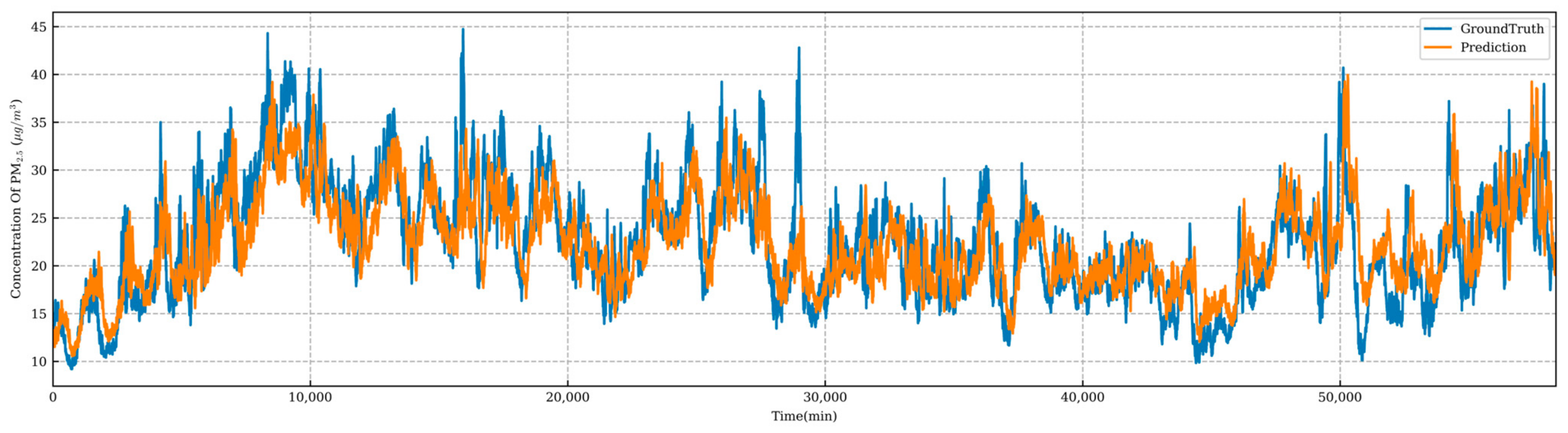
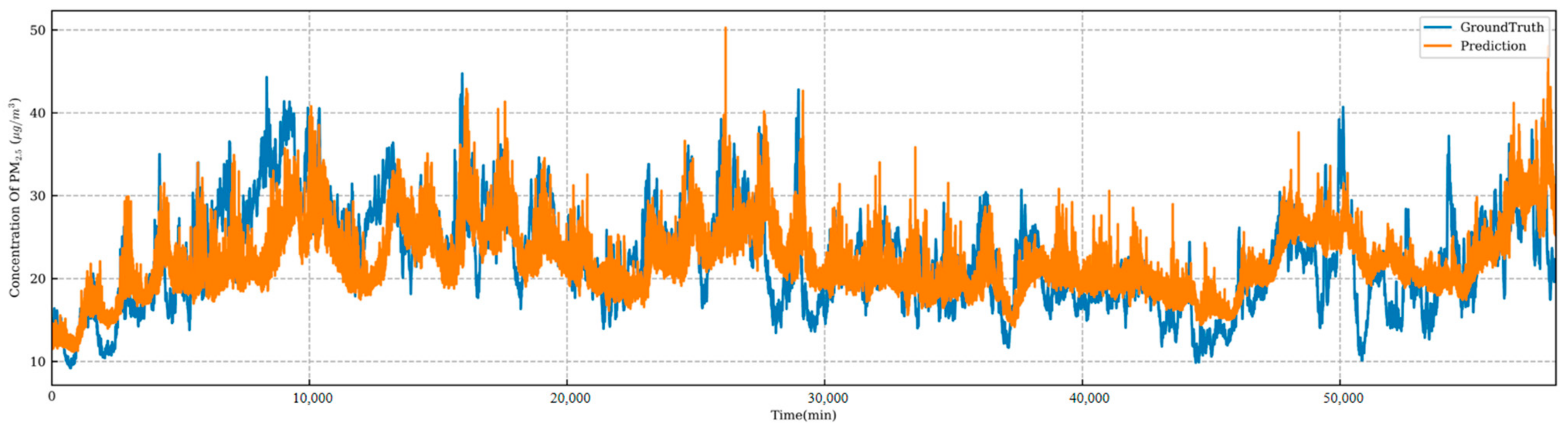
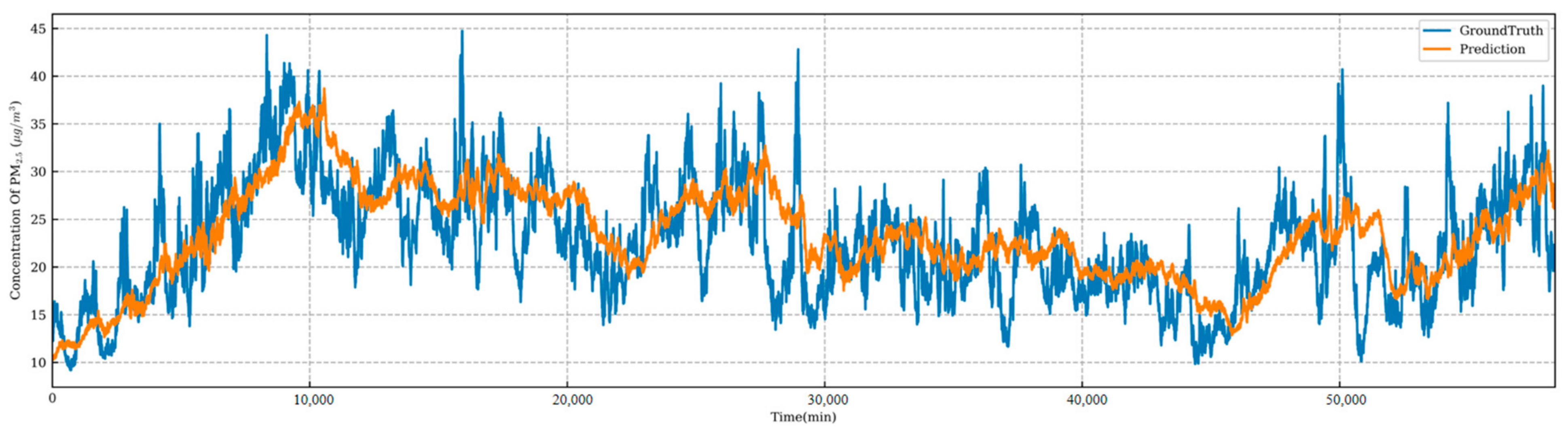
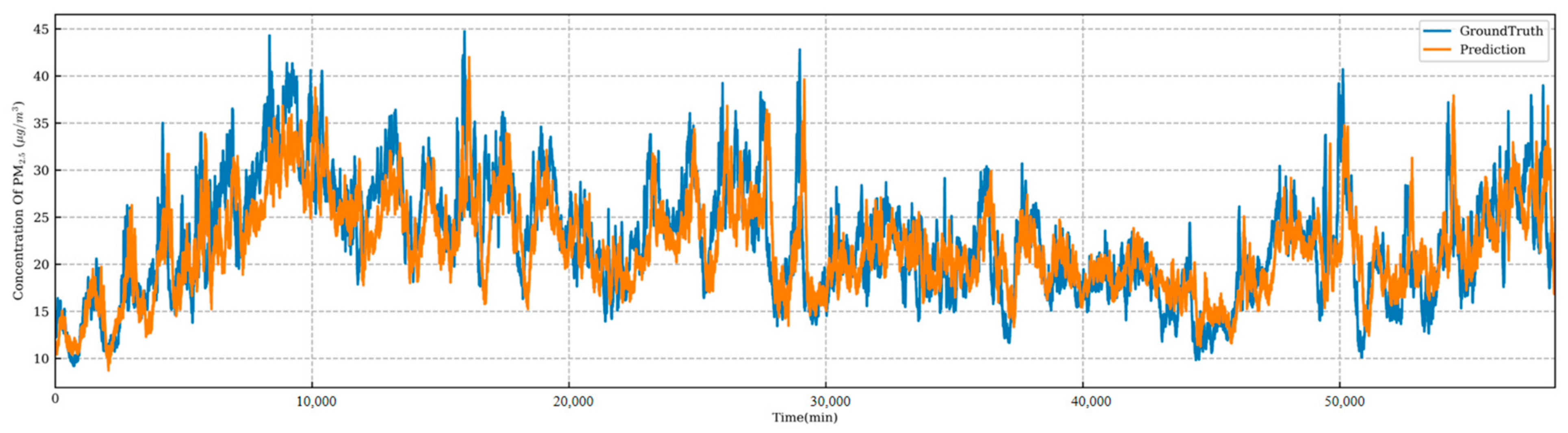
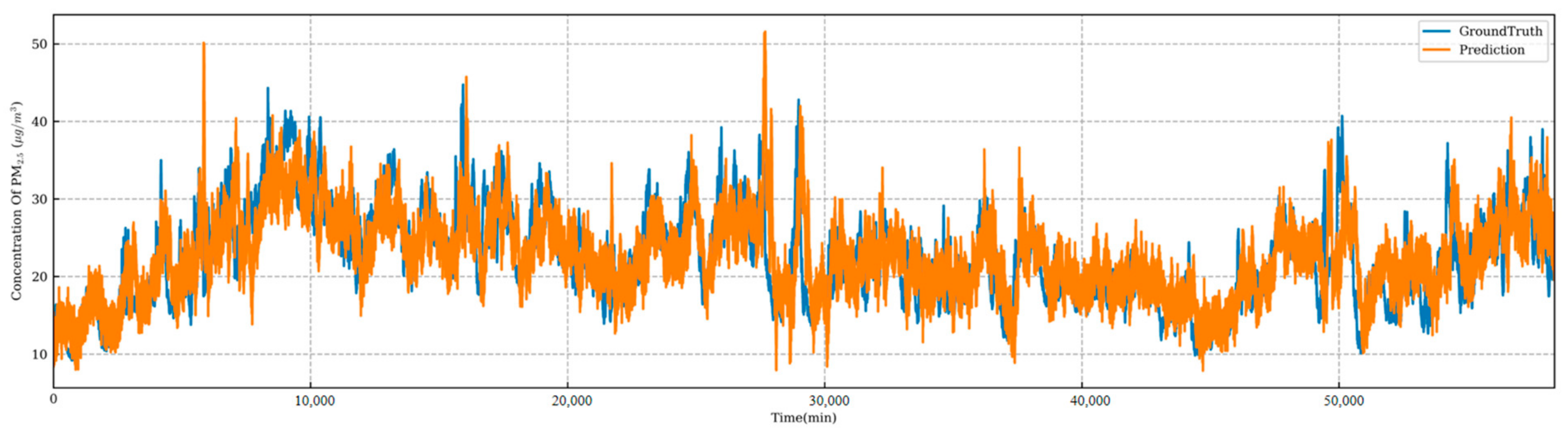
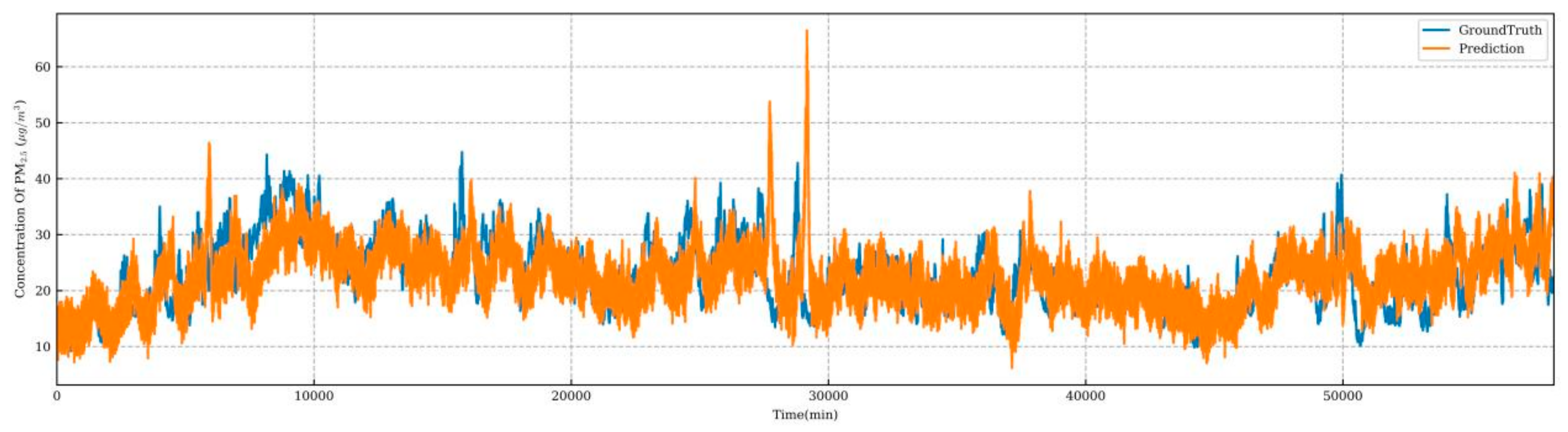
4.4. Predictive Model Performance

To enhance the smoothness of the prediction model, monitoring data were processed by calculating the average every 15 min. This approach transformed the prediction supervision information into an average for the 15-min interval from 9 h and 45 min to 10 h ahead.

Based on the current forecasting requirements, the prediction time window was adjusted to 600 min, aiming to predict pollutant concentrations for the next 6 h. The model was trained using all valid traffic and meteorological data collected from 10 August 2023 to 27 August 2024. The model’s performance is illustrated in Figure 8, where the red line indicates the PM_2.5 concentration warning threshold. A warning is issued when the predicted value exceeds this threshold.

In this task, the model achieved RMSE of 5.67, MAE of 4.18, and SMAPE of 18.56, demonstrating superior performance. The overall predictive accuracy was commendable, with the predicted values showing a high degree of consistency with the actual values. The model effectively captured the fluctuations in PM_2.5 levels and was particularly adept at predicting impending peaks in pollutant concentrations.

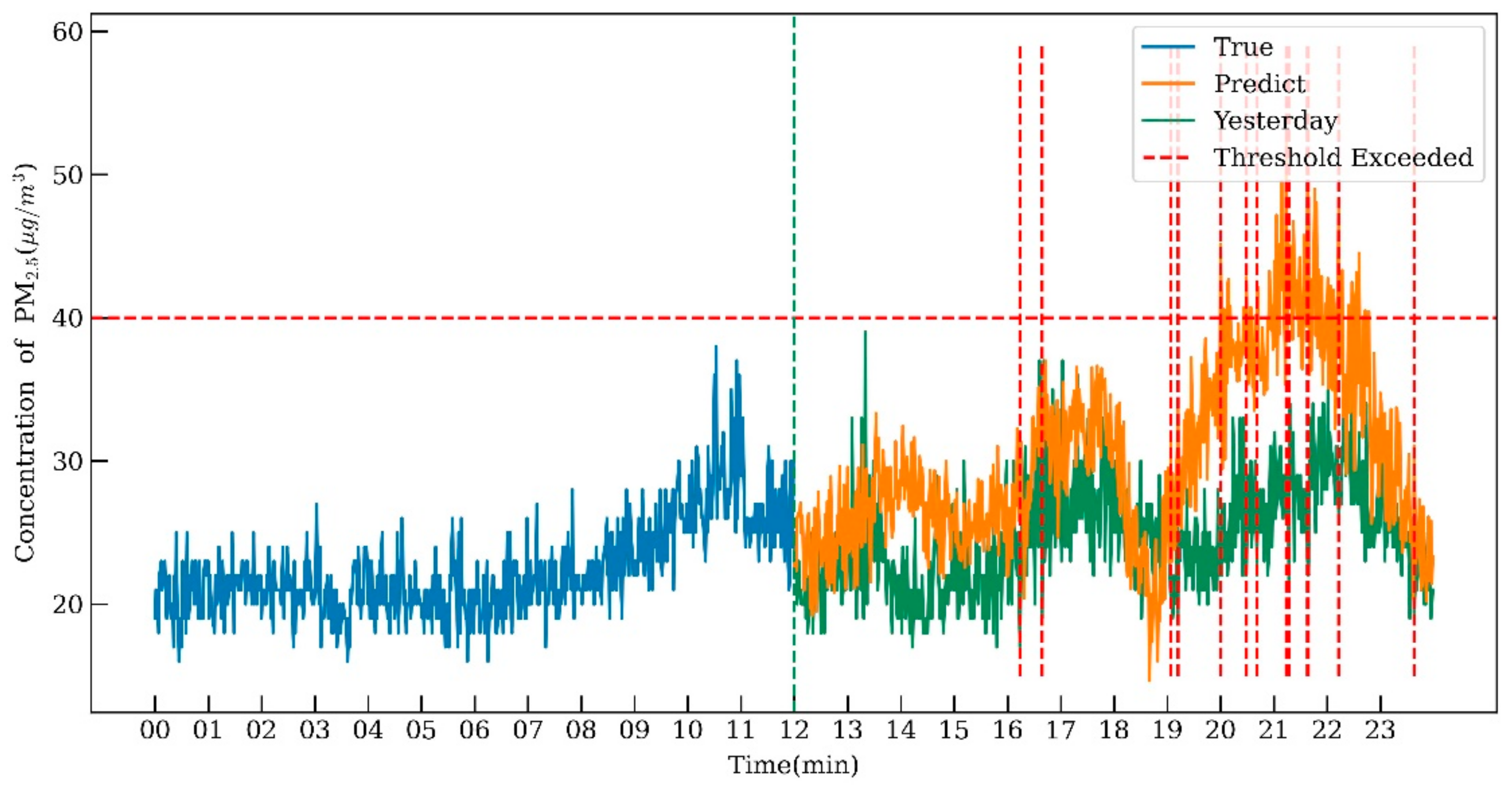
4.5. Intelligent Decision-Making Model Performance

The dust suppression operations in urban areas primarily involve water trucks and mist cannons, with decision parameters encompassing frequency, scale, and route optimization. To optimize resource utilization, we developed an intelligent water-spraying decision system based on the PM_2.5 predictions from Section 4.5. The system incorporates both fixed and dynamic thresholds for comprehensive decision-making. The fixed threshold mechanism establishes a standard PM_2.5 concentration value that, when exceeded, automatically triggers water-spraying operations. While effective, this approach alone cannot adapt to varying environmental conditions such as seasonal changes, weather patterns, geographical variations, and traffic conditions.

To address these limitations, we implement a dynamic threshold mechanism that utilizes the PM_2.5 predictions to calculate ring growth rates over $n$ collection intervals. The parameters $n$ and $k$ were optimized through extensive experimental validation. The value of $n$ was determined by analyzing the trade-off between system sensitivity and stability across different time windows, while $k$ was calibrated based on historical PM_2.5 concentration patterns and operational requirements. The dynamic threshold is computed as follows:

$${\displaystyle \frac{{\sum }_{i=1}^{n}fabs\left(Ri\right)}{n}}+dynamic threshold\ast k+min$$

(9)

where $fabs(·)$ represents the absolute value function, $Ri$ denotes the ring growth rate of monitoring data for the i-th collection interval (i = 1, 2,…, n), $k$ is the fixed threshold coefficient, and $min$ represents the minimum threshold (empirically set to 0.4 through comparative experiments).

Figure 9 demonstrates the system’s operational performance through multiple components: actual PM_2.5 concentrations from the previous day (blue curve), the current day’s predicted values (orange curve), the previous day’s reference values (green curve), with the fixed threshold indicated by a horizontal red dotted line at 40 μg/m³ and alert triggers shown as vertical red dotted lines at points where growth rates exceed the dynamic threshold. This integrated framework demonstrates robust adaptability to diverse environmental conditions while maintaining operational efficiency through scientifically grounded decision-support mechanisms. The synergistic integration of fixed and dynamic thresholds enables precise temporal and spatial optimization of dust suppression operations, facilitating proactive environmental risk management through data-driven decision-support.

5. Conclusions

This study presents the E-TSMixer, an innovative deep-learning framework for particulate matter prediction and control that achieves outperforming performance while maintaining exceptional computational efficiency. The model’s architectural innovations—a fully connected output layer and asymmetric penalty mechanism—enable robust spatiotemporal prediction capabilities, particularly excelling in critical peak value detection for environmental monitoring applications, thereby addressing a significant limitation in existing approaches. Our intelligent dual-threshold decision-making system revolutionizes urban dust control through dynamic, data-driven optimization of water truck operations. This integrated solution demonstrates superior performance over traditional methodologies, achieving substantial improvements in both prediction accuracy and operational efficiency. The system’s ability to adapt to fluctuating environmental conditions while maintaining precise control mechanisms represents a significant advancement in intelligent environmental management systems.

In the future, there are opportunities to further enhance the model’s scalability and broaden its application to other pollutants and regions. However, the current results demonstrate the model’s exceptional efficacy, establishing a solid foundation for ongoing advancements in environmental forecasting and control.

References

1. Lee, J.; Choi, J.; Kim, M.; Cho, Y.; Kim, J.; Cho, P. Verification of On-Site Applicability of Rainwater Road Surface Spraying for Promoting Rainwater Utilization and Analyzing the Fine Dust Reduction Effect. Sustainability 2024, 16, 8756. [Google Scholar] [CrossRef]
2. Yigitcanlar, T.; Kamruzzaman, M. Planning, Development and Management of Sustainable Cities: A Commentary from the Guest Editors. Sustainability 2015, 7, 14677–14688. [Google Scholar] [CrossRef]
3. Amato, F.; Querol, X.; Johansson, C.; Nagl, C.; Alastuey, A. A Review on the Effectiveness of Street Sweeping, Washing and Dust Suppressants as Urban PM Control Methods. Sci. Total Environ. 2010, 408, 3070–3084. [Google Scholar] [CrossRef]
4. Zhang, Q.; Fan, L.; Wang, H.; Han, H.; Zhu, Z.; Zhao, X.; Wang, Y. A Review of Physical and Chemical Methods to Improve the Performance of Water for Dust Reduction. Process Saf. Environ. Prot. 2022, 166, 86–98. [Google Scholar] [CrossRef]
5. Alavi, A.H.; Jiao, P.; Buttlar, W.G.; Lajnef, N. Internet of Things-Enabled Smart Cities: State-of-The-Art and Future Trends. Measurement 2018, 129, 589–606. [Google Scholar] [CrossRef]
6. Chamoso, P.; González-Briones, A.; Rodríguez, S.; Corchado, J.M. Tendencies of technologies and platforms in smart cities: A state-of-the-art review. Wirel. Commun. Mob. Comput. 2018, 2018, 3086854. [Google Scholar] [CrossRef]
7. Uyanık, G.K.; Güler, N. A Study on Multiple Linear Regression Analysis. Procedia-Soc. Behav. Sci. 2013, 106, 234–240. [Google Scholar] [CrossRef]
8. Box, G.E.P.; Pierce, D.A. Distribution of Residual Autocorrelations in Autoregressive-Integrated Moving Average Time Series Models. J. Am. Stat. Assoc. 1970, 65, 1509. [Google Scholar] [CrossRef]
9. Hurd, H.L.; Miamee, A. Periodically Correlated Random Sequences: Spectral Theory and Practice; John Wiley & Sons: Hoboken, NJ, USA, 2007; ISBN 9780470182826. [Google Scholar]
10. Shumway, R.H.; Stoffer, D.S. Time Series Analysis and Its Applications: With R Examples, 3rd ed.; Springer: Berlin/Heidelberg, Germany, 2011. [Google Scholar]
11. Chodakowska, E.; Nazarko, J.; Nazarko, Ł. ARIMA Models in Electrical Load Forecasting and Their Robustness to Noise. Energies 2021, 14, 7952. [Google Scholar] [CrossRef]
12. Byun, D.; Schere, K.L. Review of the Governing Equations, Computational Algorithms, and Other Components of the Models-3 Community Multiscale Air Quality (CMAQ) Modeling System. Appl. Mech. Rev. 2006, 59, 51. [Google Scholar]
13. Stohl, A.; Forster, C.; Frank, A.; Seibert, P.; Wotawa, G. Technical Note: The Lagrangian Particle Dispersion Model FLEXPART Version 6.2. Atmos. Chem. Phys. 2005, 5, 2461–2474. [Google Scholar] [CrossRef]
14. Spalart, P.; Allmaras, S. A One-Equation Turbulence Model for Aerodynamic Flows. In Proceedings of the 30th Aerospace Sciences Meeting and Exhibit, Reno, NV, USA, 6–9 January 1992. [Google Scholar] [CrossRef]
15. Stockie, J.M. The Mathematics of Atmospheric Dispersion Modeling. SIAM Rev. 2011, 53, 349–372. [Google Scholar] [CrossRef]
16. Joachims, T. Making Large-Scale SVM Learning Practical. In RePEc: Research Papers in Economics; Universität Dortmund: Dortmund, Germany, 1998. [Google Scholar]
17. Hochreiter, S.; Schmidhuber, J. Long Short-Term Memory. Neural Comput. 1997, 9, 1735–1780. [Google Scholar] [CrossRef]
18. Zhang, L.; Liu, P.; Zhao, L.; Wang, G.; Zhang, W.; Liu, J. Air Quality Predictions with a Semi-Supervised Bidirectional LSTM Neural Network. Atmos. Pollut. Res. 2021, 12, 328–339. [Google Scholar] [CrossRef]
19. LeCun, Y.; Bengio, Y. Convolutional networks for images, speech, and time series. In The Handbook of Brain Theory and Neural Networks; MIT Press: Cambridge, MA, USA, 1998; pp. 255–258. [Google Scholar]
20. Chen, S.A.; Li, C.L.; Yoder, N.; Arik, S.O.; Pfister, T. Tsmixer: An all-mlp architecture for time series forecasting. arXiv 2023, arXiv:2303.06053. [Google Scholar]
21. Xayasouk, T.; Lee, H.; Lee, G. Air Pollution Prediction Using Long Short-Term Memory (LSTM) and Deep Autoencoder (DAE) Models. Sustainability 2020, 12, 2570. [Google Scholar] [CrossRef]
22. Liu, Z.; Xu, X.; Luo, B.; Yang, C.; Gui, W.; Dubljevic, S. Accelerated MPC: A real-time model predictive control acceleration method based on TSMixer and 2D block stochastic configuration network imitative controller. Chem. Eng. Res. Des. 2024, 208, 837–852. [Google Scholar] [CrossRef]
23. Seng, D.; Zhang, Q.; Zhang, X.; Chen, G.; Chen, X. Spatiotemporal Prediction of Air Quality Based on LSTM Neural Network. Alex. Eng. J. 2021, 60, 2021–2032. [Google Scholar] [CrossRef]
24. Pinkus, A. Approximation Theory of the MLP Model in Neural Networks. Acta Numer. 1999, 8, 143–195. [Google Scholar] [CrossRef]
25. GB 3095-2012; Ambient Air Quality Standard. Ministry of Environmental Protection of the People’s Republic of China: Beijing, China; General Administration of Quality Supervision, Inspection and Quarantine of the People’s Republic of China: Beijing, China; China Environmental Science Press: Beijing, China, 2012.
26. Zhao, J.; Deng, F.; Cai, Y.; Chen, J. Long Short-Term Memory—Fully Connected (LSTM-FC) Neural Network for PM2.5 Concentration Prediction. Chemosphere 2019, 220, 486–492. [Google Scholar] [CrossRef]
27. Vaswani, A.; Shazeer, N.; Parmar, N.; Uszkoreit, J.; Jones, L.; Gomez, A.N.; Kaiser, L.; Polosukhin, I. Attention Is All You Need. arXiv 2023, arXiv:1706.03762. [Google Scholar]
28. Breiman, L. Random Forests. Mach. Learn. 2001, 45, 5–32. [Google Scholar] [CrossRef]
29. Zhou, T.; Ma, Z.; Wen, Q.; Sun, L.; Yao, T.; Yin, W.; Jin, R. Film: Frequency improved legendre memory model for long-term time series forecasting. Adv. Neural Inf. Process. Syst. 2022, 35, 12677–12690. [Google Scholar]
30. Campos, D.; Zhang, M.; Yang, B.; Kieu, T.; Guo, C.; Jensen, C.S. LightTS: Lightweight Time Series Classification with Adaptive Ensemble Distillation. Proc. ACM Manag. Data 2023, 1, 1–27. [Google Scholar]
31. Willmott, C.J.; Matsuura, K. Advantages of the mean absolute error (MAE) over the root mean square error (RMSE) in assessing average model performance. Clim. Res. 2005, 30, 79–82. [Google Scholar]
32. Karunasingha, D.S.K. Root Mean Square Error or Mean Absolute Error? Use Their Ratio as Well. Inf. Sci. 2021, 585, 609–629. [Google Scholar]
33. Chicco, D.; Warrens, M.J.; Jurman, G. The Coefficient of Determination R-Squared Is More Informative than SMAPE, MAE, MAPE, MSE and RMSE in Regression Analysis Evaluation. PeerJ Comput. Sci. 2021, 7, e623. [Google Scholar]
Figure 1. Structure of the TSMixer Model.
Sustainability 17 02933 g001
Figure 2. Prediction Results of the LSTM-FC Model.
Sustainability 17 02933 g002
Figure 3. Prediction Results of the Transformer Model.
Sustainability 17 02933 g003
Figure 4. Prediction Results of the FilM Model.
Sustainability 17 02933 g004
Figure 5. Prediction Results of the LightTS Model.
Sustainability 17 02933 g005
Figure 6. Prediction Results of the TSMixer Model.
Sustainability 17 02933 g006
Figure 7. Prediction Results of the E-TSMixer Model.
Sustainability 17 02933 g007
Figure 8. Prediction Performance for 6-Hour Horizon.
Sustainability 17 02933 g008
Figure 9. Example of the Intelligent Decision-Making Model Performance.
Sustainability 17 02933 g009