Abstract
Accurate prediction of extreme atmospheric conditions is essential for various scientific and engineering applications, ranging from environmental monitoring to space weather forecasting and urban climate resilience. This study introduces an empirical approach to predict maximum atmospheric pressure and temperature using an empirical model based on statistical parameters. The model incorporates key inputs such as the mean value, standard deviation, integral time scale, and a variability factor, denoted as b, to capture application-specific uncertainties. The methodology is applied to two distinct atmospheric scenarios: (i) forecasting maximum atmospheric pressure using data from 29 global monitoring stations, and (ii) predicting maximum temperature around isolated structures within unstable boundary layers, leveraging insights from Large Eddy Simulation (LES) data. The results indicate that the model performs robustly across diverse conditions, with the b parameter exhibiting a wide range of values depending on the specific atmospheric setting. The comparison between model predictions and observed data demonstrates excellent agreement, validating the model’s applicability in extreme value prediction. These findings reinforce the empirical model’s potential for integration into computational fluid dynamics (CFD) simulations, enhancing the predictive capabilities of Reynolds-Averaged Navier-Stokes (RANS) methodologies. Furthermore, the model’s ability to generalize across different atmospheric processes highlights its significance in advancing our understanding of meteorological extremes.
1. Introduction
Extreme atmospheric conditions, such as maximum pressure and temperature fluctuations, play a crucial role in shaping environmental and technological processes. Understanding and accurately predicting these extreme values is essential for applications ranging from meteorology and space weather forecasting to urban planning and climate adaptation [1,2,3,4]. However, conventional modeling approaches often struggle to capture extreme values due to the inherent complexities of turbulent flows and atmospheric variability.
Furthermore, extreme atmospheric conditions, such as maximum pressure and temperature fluctuations, play a crucial role in climate science, renewable energy forecasting, and disaster risk management. Traditional numerical weather prediction (NWP) models, such as the European Centre for Medium-Range Weather Forecasts (ECMWF) model, provide high-resolution forecasts but are computationally expensive and require substantial observational data for calibration [5]. Recently, empirical approaches have gained attention as computationally efficient alternatives that incorporate statistical relationships extracted from observed datasets [6]. However, the reliability and generalization of empirical models remain a key challenge, particularly when applied to diverse atmospheric conditions [7]. Given these challenges, integrating empirical models with numerical methods such as CFD-RANS or AI-based forecasting systems could enhance predictive accuracy and applicability across different meteorological environments [8].
Empirical models have emerged as an effective alternative to traditional numerical weather prediction methods for extreme event forecasting. These models leverage statistical properties of time series data, incorporating key parameters such as mean values, variance, integral time scales, and fluctuation intensities to estimate maximum values. Recent studies have successfully applied empirical models to a variety of domains, including hydrogen combustion, and pollutant dispersion in urban environments [9,10]. However, their application to atmospheric pressure and temperature extremes remains an area of active research.
This study presents a unified empirical approach for predicting maximum atmospheric pressure and temperature using an empirical model. The proposed methodology is applied to two different cases:
- Maximum atmospheric pressure prediction—Utilizing data from 29 global monitoring stations, the model estimates the highest recorded atmospheric pressure based on key statistical parameters. The findings highlight the variability of the b parameter, which accounts for local atmospheric conditions, with values ranging from 0.22 to 6.27, underscoring the need for location-specific adjustments.
- Maximum temperature prediction—The model is validated against Large Eddy Simulation (LES) data for an unstable boundary layer around an isolated building. The results demonstrate excellent agreement between the model’s predictions and LES data, reinforcing its applicability to urban microclimates and atmospheric boundary layer studies [11,12,13].
Recent advancements in weather forecasting have increasingly incorporated artificial intelligence (AI) and machine learning techniques to enhance the prediction of extreme atmospheric conditions. Notably, Google’s DeepMind introduced GenCast, an AI-based model that outperforms traditional systems like the European Centre for Medium-Range Weather Forecasts (ECMWF) in forecasting extreme weather events up to 15 days in advance. Similarly, researchers have developed FourCastNet, an AI-driven high-resolution weather model capable of predicting extreme events such as heatwaves and hurricanes with greater speed and accuracy compared to conventional models. These developments underscore the potential of integrating AI methodologies in atmospheric modeling to improve the accuracy and efficiency of extreme weather predictions.
A critical aspect of this study is the role of the b parameter of the empirical model, which introduces application-specific corrections based on environmental conditions. Previous applications of the empirical model have shown that b is highly sensitive to local meteorological and geometric factors, affecting the accuracy of extreme value predictions. Addressing this uncertainty is essential for enhancing the model’s predictive robustness, particularly in complex environments such as unstable atmospheric boundary layers [14,15].
This research contributes to the field of extreme atmospheric event prediction in several key ways:
- Expansion of the empirical model: Previous studies have focused on applying empirical models to individual domains such as hydrogen combustion and pollutant dispersion. This work extends the methodology to both atmospheric pressure and temperature extremes, demonstrating its broad applicability.
- Integration with CFD-RANS and LES: While empirical models typically operate independently, this study explores their integration with CFD methodologies, enhancing their utility in engineering applications such as urban heat mitigation and environmental risk assessment [16,17].
- Enhanced understanding of the b parameter: The study investigates the variability and sensitivity of b, providing new insights into how local conditions influence model accuracy. This is particularly relevant for applications requiring precise extreme value predictions, such as space weather forecasting and urban climate modeling [18].
By addressing these aspects, this research aims to refine existing methodologies for extreme value prediction, offering a computationally efficient and broadly applicable tool for atmospheric sciences. The results demonstrate that the empirical model can serve as a valuable addition to conventional numerical weather prediction models, improving the accuracy of extreme event forecasting while reducing computational complexity.
Furthermore, the prediction of extreme atmospheric conditions, such as maximum pressure and temperature, is a complex problem that requires a robust modeling framework. While empirical models provide a practical approach to estimating extreme values, they can be further enhanced through their integration with well-established CFD techniques, such as RANS and LES.
RANS models solve the time-averaged Navier-Stokes equations, making them computationally efficient for predicting mean flow characteristics in atmospheric boundary layers. However, these models often struggle to capture transient fluctuations that influence extreme conditions. LES, on the other hand, resolves larger turbulent eddies directly while modeling the smaller ones, making it more suitable for capturing the dynamic nature of extreme events. By integrating empirical approaches with RANS or LES, a more comprehensive prediction framework can be established.
Previous studies have demonstrated that empirical formulations can be successfully embedded in CFD methodologies. For instance [19], incorporated an optimized beta distribution within the RANS framework to predict wind speed probabilities in the atmospheric surface layer. Their results showed a strong agreement between modeled and experimental data, validating the capability of such hybrid approaches in complex atmospheric conditions. The present study follows a similar philosophy by leveraging an empirical model to estimate extreme pressure and temperature values, which can be further enhanced through its potential integration with RANS-based turbulence models.
Recent advancements in extreme weather prediction have leveraged machine learning techniques, particularly convolutional neural networks (CNNs) and time series neural networks, to enhance forecasting accuracy. While these methods have demonstrated success in capturing nonlinear dependencies and complex atmospheric patterns, they often require extensive training datasets, computational resources, and careful hyperparameter tuning to achieve optimal performance.
The empirical model proposed in this study does not aim to compete with machine learning approaches but rather to complement them by providing a computationally efficient alternative that captures key statistical properties of extreme atmospheric events. Unlike machine learning models, which primarily rely on data-driven learning, this empirical approach incorporates physically relevant statistical parameters such as the mean value, standard deviation, integral time scale, and fluctuation intensity. These parameters introduce interpretability and robustness to the model’s predictions, making it particularly useful in scenarios where high-fidelity data for training machine learning models may be limited or where rapid, low-computation predictions are required.
Additionally, the empirical model offers potential integration with existing machine learning frameworks. For example, the parameter b, which encapsulates local atmospheric variability, could serve as an additional feature in hybrid models that combine statistical and deep learning approaches. Future work could explore such integrations to leverage the strengths of both methodologies, ultimately improving the accuracy and generalizability of extreme weather predictions.
By positioning the empirical model as a complementary tool rather than a direct competitor to machine learning techniques, this study broadens the spectrum of available methods for predicting maximum atmospheric pressure and temperature. This approach enhances the flexibility of predictive models, allowing for adaptability across diverse atmospheric conditions with reduced computational overhead.
The study presents an empirical model for predicting extreme atmospheric conditions, specifically maximum atmospheric pressure and temperature. This work aligns with sustainability goals in several key ways:
1.1. Urban Climate Resilience & Sustainable Infrastructure
The accurate prediction of maximum temperature fluctuations in urban environments is crucial for mitigating urban heat island (UHI) effects, improving thermal comfort, and optimizing building energy efficiency. By integrating the model with CFD-RANS methodologies, urban planners and engineers can make more informed decisions regarding sustainable building design and climate adaptation strategies.
1.2. Renewable Energy Optimization
Extreme weather events, including temperature and pressure anomalies, impact the performance of renewable energy systems such as wind and solar power. The model enhances forecasting accuracy, enabling better grid integration of renewables and reducing energy losses, thereby supporting a more sustainable energy infrastructure.
1.3. Environmental Monitoring & Climate Adaptation
By improving extreme event prediction, the methodology supports environmental sustainability through enhanced risk assessment of heatwaves, pressure-related storm intensities, and atmospheric turbulence effects. This allows for proactive climate adaptation measures, benefiting both ecosystems and human well-being.
1.4. Computational Efficiency & Reduced Carbon Footprint
Unlike conventional high-resolution numerical simulations, the empirical model provides accurate predictions with significantly lower computational demands. This reduces energy consumption associated with large-scale simulations, contributing to sustainability in computational research and engineering applications.
1.5. Cross-Disciplinary Applications for Sustainable Development
The flexibility of the model extends to multiple scientific domains, including air quality monitoring, extreme weather forecasting, and even space weather prediction. These applications contribute to broader sustainability efforts by enhancing environmental protection policies and disaster preparedness strategies.
The remainder of this paper is structured as follows: Section 2 presents the methodology, detailing the empirical model formulation and statistical parameter selection. Section 3 discusses the datasets used for atmospheric pressure and temperature analysis. Section 4 provides a comparative evaluation of model predictions against measured data, highlighting key findings. Finally, Section 5 summarizes the conclusions and outlines future research directions, particularly in refining the b parameter for enhanced model accuracy across diverse atmospheric conditions.
2. Model Description and Methodology
This study follows a structured approach to developing an empirical model for extreme atmospheric conditions. The methodology consists of four key steps: (1) dataset selection and preprocessing, (2) statistical parameter estimation, (3) model formulation, and (4) validation against observational and simulated data. Unlike traditional NWP models, which rely on dynamical equations, this empirical approach captures statistical characteristics of atmospheric variability, making it computationally efficient and adaptable for integration into hybrid modeling frameworks.
In the proposed empirical model, the maximum time-averaged value of the variable (pressure/temperature) Vmax(Δτ) in the interval Δτ is approximated as follows:
where is the mean value and I is the fluctuation intensity which is calculated as follows:
The parameter ν in Equation (1) plays a critical role in determining the scaling behavior of the maximum concentration predictions over different time intervals. It is linked to the integral turbulence time scale and governs how the maximum concentration decreases as the averaging time increases. Previous studies on atmospheric dispersion and turbulence characteristics indicate that ν is highly dependent on the nature of the turbulent flow and the exposure time of interest.
A key reference supporting the selection of ν = 0.3 is the work of [20], who analyzed concentration fluctuations and their scaling in turbulent boundary layers. Their study, based on data from the FLADIS field experiments, demonstrated that for ground-level releases under neutral atmospheric conditions, ν typically varies within the range of 0.2 to 0.5. Specifically, their findings showed that a representative value of ν = 0.3 provides a reasonable approximation for the behavior of maximum concentration fluctuations over different time averaging intervals. The value ν = 0.3 was found to be consistent with experimental data from large-scale field experiments, confirming its robustness in describing the relationship between short-term peak concentrations and long-term averages. Given the relevance of this formulation in atmospheric turbulence and dispersion modeling, we adopt the value ν = 0.3 in our study, aligning with the established literature on maximum concentration estimation in turbulent flows.
The variable V′ represents the fluctuating component of the atmospheric variable V, which can be either pressure or temperature, around its mean value.
TV is the integral time scale derived from the autocorrelation function RV(τ) and these are calculated as follows:
The parameter b incorporates application-specific uncertainties, which depend on local atmospheric conditions. The values of b have been observed to range between 0.22 and 6.27 in case of pressure, as described in the present study and previous works [9].
In case of temperature, the temporal resolution of the dataset used for validating the empirical model is characterized by a constant timestep (Δτ) of 0.001 s. This fine resolution ensures accurate capturing of transient phenomena within the unstable boundary layer, allowing for precise calibration of the model parameters. The timestep value is consistent across all simulations, reflecting a uniform temporal discretization.
The history of the empirical model is presented in detail in [9]. In all the previous works the parameter ν was kept constant and equal to 0.3 and all the uncertainties were reflected to the parameter b.
The empirical model employed in this study is well-suited for integration into the RANS (Reynolds-Averaged Navier-Stokes) methodology, as it has been demonstrated to enhance prediction capabilities for maximum pollutant concentrations in complex geometries such as urban environments. As described in the literature [10], the empirical model can be incorporated into CFD simulations by parameterizing turbulent characteristics and dispersion timescales. Beyond atmospheric pressure, this study focuses on the application of the model in thermally unstable atmospheric layers, highlighting its potential for broader applications in maximum value predictions.
Specifically, the model estimates the maximum concentration using inputs such as mean concentration, fluctuation intensity, and correlation timescale. Its integration into a CFD-RANS framework does not require additional transport equations but instead utilizes the existing turbulence equations, ensuring computational efficiency and predictive accuracy.
The model’s ability to integrate into RANS frameworks underscores its value, as it provides tools for reliable predictions over extended time periods and diverse scenarios. Although this work does not include direct RANS simulations, the results demonstrate that the model can support RANS-based applications effectively.
The parameter ‘b’ captures application-specific uncertainties and has shown versatility across different scientific fields. As validated in Atmosphere [9], the model’s accuracy relies heavily on the calibration of ‘b’ to reflect the unique dynamics and variabilities within each application, ranging from urban microclimates to hydrogen safety.
Unlike conventional RANS approaches, which often struggle with accurate peak temperature predictions due to their inherent simplification of turbulent fluctuations, this model integrates LES-calibrated parameters to maintain fidelity in extreme value prediction. This integration with CFD-RANS provides a robust framework, making it suitable for applications that demand high precision in unstable boundary layer conditions, thereby broadening the applicability of RANS in temperature-sensitive domains.
In this study, the parameter b was calibrated using LES data for an unstable boundary layer around an isolated building. This calibration ensures that the model’s predictions align closely with the maximum temperature values observed in high-fidelity simulations, while also accounting for the inherent variability in turbulent flow conditions.
2.1. Parameterization and Physical Interpretation of Parameter ‘b’
The parameter b serves as an empirical adjustment factor, encapsulating the influences of environmental and geometric conditions that are not explicitly modeled. This approach is common in atmospheric science, where certain sub-grid scale processes are parameterized to simplify complex models.
Furthermore, the parameter b serves as an empirical correction factor that accounts for application-specific uncertainties, reflecting the influence of local atmospheric dynamics and geometric conditions on extreme value predictions. Its variability is primarily driven by the interaction between turbulent flow structures and thermodynamic processes, particularly in unstable atmospheric boundary layers. In complex environments, such as urban microclimates or regions with significant topographical variations, the value of b adapts to changes in turbulence intensity, thermal stratification, and energy dissipation mechanisms. The parameter encapsulates the subgrid-scale effects that are not explicitly resolved in the empirical formulation, making it a critical component for improving model accuracy. Previous studies have indicated that the sensitivity of b to local conditions suggests its potential for calibration using real-time meteorological data, enabling dynamic adjustments based on evolving atmospheric states. Further refinement of b through data assimilation techniques and integration with high-resolution numerical models could enhance its robustness across diverse environmental conditions.
In atmospheric modeling, parameterization is a standard technique used to represent processes that occur at scales smaller than the model’s resolution or are too complex to be physically represented. For instance, cloud formation, convection, and turbulence are often parameterized to account for their effects without modeling the detailed physics explicitly. This method involves introducing empirical parameters that adjust the model to align with observed data, thereby improving its predictive capabilities.
Several renowned atmospheric models employ empirical parameters to enhance their accuracy:
- NRLMSISE-00 Model: This empirical model of Earth’s atmosphere incorporates parameters to predict temperature and density variations up to the exosphere. It adjusts for factors like solar activity and geomagnetic indices to provide accurate atmospheric profiles.
- Monin–Obukhov Similarity Theory: This theory introduces the Obukhov length (L), a parameter that characterizes the relative contributions of buoyant and shear production of turbulence in the surface layer. It serves as a scaling parameter to describe the effects of stability on turbulence and is widely used in boundary-layer meteorology.
The variability of parameter b highlights the inherent uncertainties in modeling complex atmospheric processes. To mitigate this, a sensitivity analysis can be conducted to assess how variations in b impact model outputs. Additionally, calibrating b using extensive observational data across diverse environmental conditions can enhance its robustness and reduce predictive variability.
2.2. Pseudocode for the Empirical Model Implementation
The implementation of the empirical model follows a systematic approach, beginning with data import and preprocessing. Initially, atmospheric pressure or temperature data is loaded, and anomalies are computed by subtracting the mean value from each data series. Following this, the autocorrelation function (ACF) of the anomaly series is calculated for each station or sensor. The integral time scale (TV) is then derived by identifying the point where the ACF becomes negative and integrating the function accordingly.
Once the time scale is determined, key statistical parameters such as the mean value, standard deviation, and fluctuation intensity (I) are computed. The next step involves estimating the parameter b, which is calculated using the formula:
Using this parameter, the empirical model predicts the maximum atmospheric pressure or temperature by applying the following equation:
To analyze the distribution of b across different stations or sensors, a histogram is generated, offering insights into its variability. Additionally, the predicted maximum pressure or temperature values are compared against observed maximum values using scatter plots, ensuring the accuracy of the model. This structured approach provides a computationally efficient methodology for predicting extreme atmospheric conditions while minimizing the need for complex numerical simulations.
3. The Selected Databases
The dataset used in this study comprises atmospheric pressure measurements from 29 monitoring stations distributed across multiple climate zones. These stations were selected to represent a variety of geographic locations, including coastal, continental, and high-altitude sites, to capture diverse atmospheric conditions. However, limitations exist due to uneven station distribution, with a larger concentration in mid-latitude regions and fewer datasets available for tropical and polar environments. Previous studies have emphasized the importance of incorporating a broader geographic range to improve the robustness of empirical models [21]. In future work, expanding the dataset to include additional meteorological stations, particularly from underrepresented regions, could enhance the generalizability of the findings.
3.1. Atmospheric Pressure
For the validation and calibration of the proposed empirical model, a comprehensive dataset of atmospheric pressure measurements was gathered from global monitoring stations. This dataset was chosen due to its extensive coverage and the high temporal resolution of the atmospheric pressure data it offers. The pressure measurements are crucial as they directly influence the predictions of maximum atmospheric pressure, which is the focus of this study.
The dataset spans the entirety of 2022, covering the period from 1 January 2022, 00:00:00 UTC to 31 December 2022, 12:00:00 UTC. During this period, atmospheric pressure data from 29 stations across the globe were collected continuously. These stations are part of a global network that provides real-time measurements of atmospheric conditions, making this dataset ideal for a robust analysis of atmospheric pressure variations.
Each station’s data were pre-processed to eliminate any irregularities or missing entries that could skew the results. Following the pre-processing, an averaging period (Δτ) of 12 h was selected for the analysis. This choice was based on previous studies that identified 12-h windows as optimal for capturing meaningful variations in atmospheric pressure while maintaining a manageable dataset size for computational analysis.
The stations exhibited considerable variability in the key parameter of interest: the autocorrelation time scale (TV) and the variance of the atmospheric pressure measurements. This variability is crucial for testing the flexibility and robustness of the empirical model across different environmental and atmospheric conditions. The model also incorporated the fluctuation intensity (I), which quantifies the degree of deviation from the mean value of the atmospheric pressure, further refining its predictive capacity.
The primary model parameter, denoted as b, was found to exhibit substantial differences among the 29 stations, with values ranging from as low as 0.22 to a maximum of 6.27. These variations highlight the influence of local geomagnetic and atmospheric conditions on atmospheric pressure measurements, which the model successfully accounts for. The wide range of b values underscores the importance of considering station-specific characteristics when applying the empirical model to different regions.
In summary, the dataset selected for this study not only offers comprehensive global coverage but also ensures that the model can be rigorously tested against diverse environmental conditions. By leveraging the wealth of data provided by the monitoring stations, the study is able to validate the model’s predictions of maximum atmospheric pressure with a high degree of confidence, ensuring its applicability to both scientific research and practical applications such as weather forecasting and environmental monitoring.
Table 1 provides a summary of the neutron monitor stations utilized in this study. The data were retrieved from the NMDB database, ensuring consistency and reliability for the analysis.

Table 1.
The neutron monitor stations utilized in this study. The data were retrieved from the NMDB database.
The dataset used in this study was obtained from the Neutron Monitor Database (NMDB) (www.nmdb.eu, accessed on 1 January 2024). It contains time series of atmospheric pressure measured at multiple neutron monitoring stations worldwide. The data were retrieved in hourly intervals and processed to obtain 12-h averaged values to reduce noise and highlight long-term trends.
One of the key concerns raised regarding this study is the geographic representativeness of the dataset, given that the model validation is based on atmospheric pressure data from 29 global monitoring stations. It is important to highlight that all available stations from the NMDB were utilized, ensuring the most comprehensive dataset accessible for this analysis. The NMDB provides high-quality, long-term observations of atmospheric pressure across diverse geographical locations, covering a wide range of latitudes and altitudes.
While the current dataset represents a variety of climatic conditions and regional influences, we acknowledge that additional monitoring stations, particularly in regions with extreme weather variability (e.g., tropical and polar climates), could further strengthen the model’s generalizability. However, expanding the dataset beyond the NMDB would require integrating data from different observational networks, each with varying measurement standards and temporal resolutions, potentially introducing inconsistencies.
Future studies could explore alternative global datasets, such as those from meteorological agencies or reanalysis products, to enhance the spatial diversity of validation cases. Despite this limitation, the results demonstrate the empirical model’s robustness across distinct atmospheric environments, supporting its applicability to a wide range of meteorological conditions.
Furthermore, the dataset consists of timestamps and corresponding atmospheric pressure values from different neutron monitor stations. Missing or erroneous values are represented as “null” in the original dataset and were replaced with NaN (Not a Number) during preprocessing. The data were then converted into a numerical format, and the time column was set as the index for time series analysis.
To illustrate the dataset, Figure 1 presents the atmospheric pressure time series for three selected stations. This visualization highlights the variability of atmospheric pressure across different locations and the temporal resolution of the dataset.
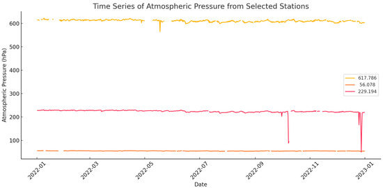
Figure 1.
Time series of atmospheric pressure from selected stations.
3.2. Description of LES Experiments
In [13], a series of LES experiments were conducted to investigate the airflow and thermal fields around an isolated building within an unstable boundary layer. The experiments aimed to evaluate the performance of polyhedral meshes compared to hexahedral meshes under non-isothermal conditions, which are typical in real urban environments due to meteorological and anthropogenic factors.
The building model had dimensions of 0.08 m × 0.08 m × 0.16 m (width × depth × height) and was placed within a computational domain of 12.5H (length) × 7.5H (width) × 6.25H (height), where H represents the building height. The computational domain was designed to simulate an unstable boundary layer, generated by aluminum plates placed on the wind tunnel floor to induce turbulence. The surface temperature of the ground was set to 45.8 °C, while the inflow conditions were determined by a precursor simulation to account for the velocity and temperature fluctuations.
The simulations were performed using a second-order central differencing scheme, while the Smagorinsky model was employed to model subgrid-scale stresses. Boundary layer meshes were introduced in certain cases to assess their impact on accuracy. Key variables like mean velocity, turbulent kinetic energy, and temperature were validated against wind tunnel experimental data.
The study evaluated the performance of polyhedral meshes in predicting the wind and temperature fields around the isolated building. Polyhedral meshes with additional boundary layer meshes near the ground provided improved accuracy in the temperature field, particularly in the standard deviation of temperature. Specifically, cases with uniform boundary layer mesh exhibited a 20% reduction in relative error for temperature standard deviation near the ground compared to cases without boundary layer meshes. The use of the standard Smagorinsky model for subgrid-scale modeling further enhanced the simulation accuracy in the turbulent flow domain.
The chosen experimental setup, which simulates a realistic urban environment through non-isothermal conditions, captures essential features of the flow and thermal field interactions. While it is recognized that LES inherently involves a degree of uncertainty, particularly in boundary layer turbulence, the detailed nature of the simulation—such as the use of polyhedral meshes for efficiency and accuracy—offers a solid foundation for model validation.
The conditions simulated by the LES experiments are closely aligned with those found in practical applications, such as urban planning and building design in climates with unstable boundary layers. The LES data therefore serve not only as a validation tool but also as an appropriate benchmark for understanding the model’s applicability to real-world problems.
The computational domain and boundary conditions for the reference LES case are described in detail in [13]. The domain includes a 1:1:2 idealized building within an unstable boundary layer, with dimensions extending to 12.5H in the stream-wise direction, 7.5H laterally, and 6.25H vertically, where H is the building height. The upstream length from the inlet boundary to the building was 2H, and the downstream length to the outlet boundary was 10H.
Boundary conditions were implemented based on the Spalding wall function for velocity and the Jayatilleke wall function for temperature, ensuring accurate representation of wall shear stress and heat flux. The ground temperature was set to 45.8 °C, consistent with the experimental setup. For further details regarding the domain and boundary condition configurations, please refer to [13].
4. Results and Discussion
4.1. Atmospheric Pressure
Figure 2 presents the histogram of the parameter b for all the stations. Most of the results are between the values 0.5 and 1.0. The maximum value is equal to 6 and this was also the finding of the model for the wind speed in the indoor and outdoor environments.
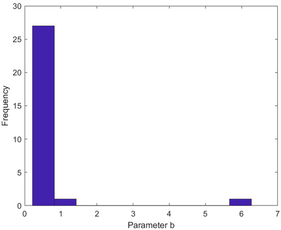
Figure 2.
The variation of b values across stations. The parameter b reflects application-specific uncertainties, influenced by local atmospheric conditions, with values ranging between 0.22 and 6.27.
Figure 3 presents the maximum pressure (Pa) of the model versus the measurements. It is clear that all the points are on the 1 to 1 line supporting the robustness of the model. Also, Table 2 presents the values for each station that was used for the derivation of Figure 2 and Figure 3.
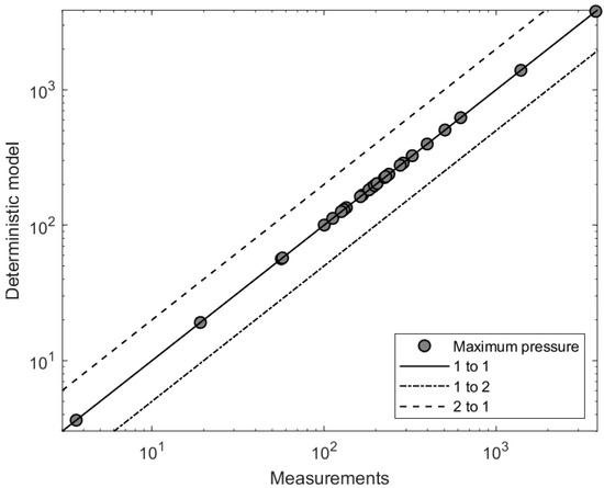
Figure 3.
Comparison of predicted and observed maximum atmospheric pressure values (Pa).
Table 2.
Overview of variables used in the model, including ΜΕAΝ (mean atmospheric pressure, Pa), I (fluctuation intensity, unitless), TP (integral time scale, s), and b (uncertainty parameter, unitless).
The excellent agreement of the proposed model with the observed values demonstrates its ability to capture critical factors influencing maximum atmospheric pressure. Previous applications of the model [9] also showed its adaptability to different scientific domains, including hydrogen combustion, shipping emissions, and urban wind flows. This study revealed that the value of the parameter b appropriately adjusts to the conditions of each application, resulting in accurate predictions.
The comparison of the model’s results with data from other fields supports the argument that the observed agreement is not coincidental but stems from the empirical nature of the model and its ability to capture the critical parameters influencing extreme phenomena. For example, in the hydrogen combustion study, the model’s success in accurately predicting maximum concentrations highlights its stability and reliability.
The reference to the study [9] also provides evidence that the parameter b is influenced by the complexity of physical processes, as demonstrated by its higher values in shipping emissions. This flexibility makes the model ideal for use in various applications, ranging from cosmic ray intensity predictions to atmospheric pressure forecasting.
4.2. Atmospheric Temperature
In this section, we present the analysis of the results obtained from the empirical model validated against LES data. The objective is to assess the model’s performance in predicting the maximum temperature around an isolated building within an unstable boundary layer and to quantify the impact of the uncertainty in parameter ‘b’.
4.2.1. Maximum Temperature Prediction
The prediction of the maximum temperature (K), which is a critical output of the empirical model, is presented in Figure 4. The model aligns well with the LES data. This study does not include RANS simulations due to its focus on validating the empirical model using high-fidelity LES data. Future work will explore the integration of the empirical model into RANS simulations to evaluate its predictive capabilities in scenarios involving extreme temperatures. Such comparisons, including RANS-only, RANS + empirical model, and LES data, will provide deeper insights into the model’s effectiveness.
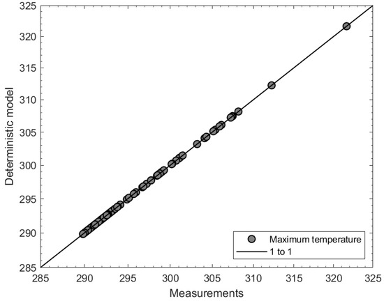
Figure 4.
Graph showing the comparison of maximum temperature predictions (K) from the empirical model and LES simulations.
4.2.2. Sensitivity of Parameter “b”
The parameter “b” plays a crucial role in the accuracy of the proposed model for predicting maximum temperature. To investigate its impact, we conducted a sensitivity analysis using data from different heights (z = 0H, z = 0.025H, z = 0.25H).
The distribution of parameter “b” is shown in Figure 5a–c for the datasets from the respective heights. The histograms reveal that the values of “b” exhibit significant variation, indicating that the model’s sensitivity heavily depends on the selection of this parameter. Specifically:
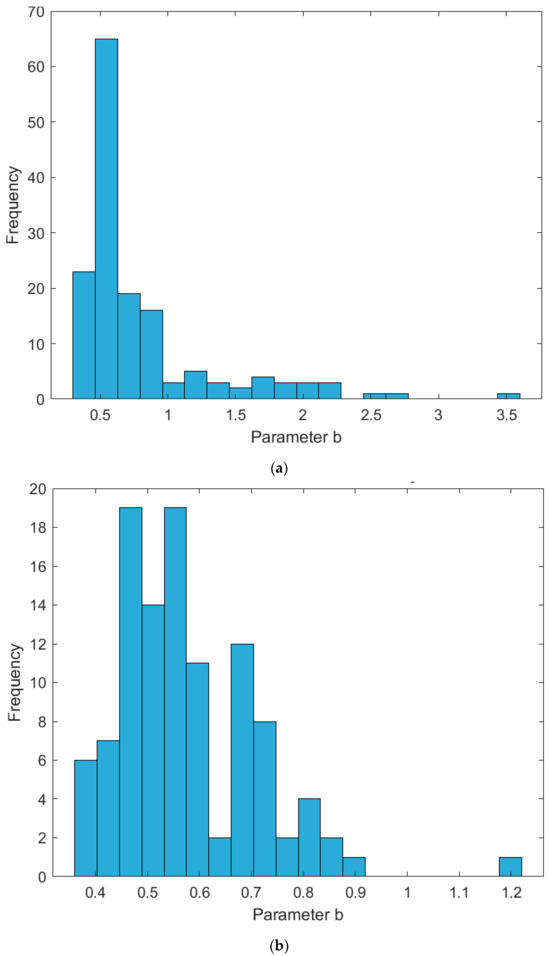
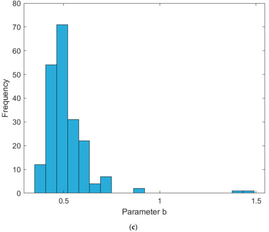
Figure 5.
(a–c) Histograms of parameter “b” for different heights.
The comparison between measured maximum temperatures (K) and model predictions is presented in Figure 6a–c. From these plots, we observe:
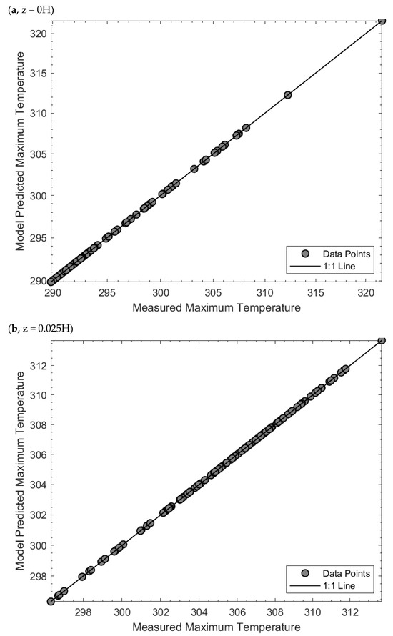
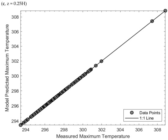
Figure 6.
(a–c) Comparison of model predictions and measured maximum temperatures (K).
- Good agreement between model predictions and measurements, with most data points aligning closely with the 1:1 diagonal.
- Significant accuracy in predicting maximum values, highlighting the utility of “b” in fine-tuning the model.
This section presents also the analysis of the sensitivity of parameter ‘b’ in relation to the sensor positions and its distribution across different heights (z = 0H, z = 0.025H, and z = 0.25H). The analysis aims to address the variability of ‘b’ and its dependence on spatial coordinates.
The following figures (Figure 7, Figure 8 and Figure 9) illustrate the relationships between parameter ‘b’ and the spatial coordinates. The analysis revealed the following key findings regarding the sensitivity of parameter ‘b’:
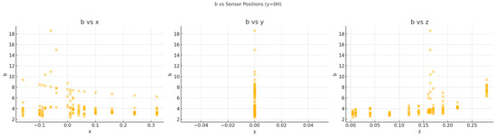
Figure 7.
Scatter plots showing ‘b’ vs. positions for y = 0H.
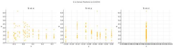
Figure 8.
Scatter plots showing ‘b’ vs. positions for z = 0.025H.
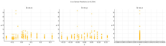
Figure 9.
Scatter plots showing ‘b’ vs. positions for z = 0.25H.
- At y = 0H, parameter ‘b’ shows a moderate positive correlation with z (0.48) and a weak negative correlation with x (−0.20).
- At z = 0.025H and z = 0.25H, the correlations with x and y are weak or negligible, indicating a lesser dependence of ‘b’ on these coordinates at higher levels.
- The distribution of ‘b’ varies significantly across different heights, with higher variability observed at y = 0H.
The parameter ‘b’ was observed to exhibit spatial variation across the domain, particularly in relation to the streamwise (x), spanwise (y), and vertical (z) coordinates. This variation is intrinsically linked to the inflow conditions and the dynamics of the unstable boundary layer. Specifically, the influence of thermal stratification and buoyancy-driven flows manifests as heightened variability of ‘b’ near the ground and in the wake of the building, where thermal gradients and turbulence intensity are most pronounced.
At lower heights (z), where the ground heating effect dominates, ‘b’ tends to increase due to stronger buoyancy effects coupled with mechanical turbulence. Conversely, at higher elevations (z > H/2), the influence of thermal gradients diminishes, leading to a stabilization of ‘b’. Furthermore, near the leading edges of the building, the inflow’s characteristics, such as velocity gradients and thermal stratification, play a critical role in shaping the observed values of ‘b’.
These findings align with results from LES studies under non-isothermal conditions (e.g., [15,22]), which highlight the critical role of buoyancy in defining turbulent structures in urban environments. The parameter ‘b’ thereby acts as a proxy for the localized interplay of thermal and mechanical turbulence, offering insights into pollutant dispersion and thermal comfort in urban areas.
The empirical parameter b acts as an application-specific correction factor that captures the inherent variability of turbulent and thermal processes in complex environments. Its variation across different heights, as shown in the figures, suggests that b is influenced by the local energy distribution in the boundary layer.
In an unstable boundary layer, buoyancy-driven turbulence can lead to stronger fluctuations near the ground, where surface heating is more intense. This is reflected in the higher values of b observed at lower heights. Conversely, at greater heights, where turbulent mixing is more homogeneous, b exhibits lower variability. This phenomenon aligns with established atmospheric studies, which indicate that peak temperature fluctuations are more pronounced closer to the surface due to the combined effects of mechanical and thermal turbulence [15].
The dependence of b on flow and thermal characteristics suggests that it can serve as a turbulence-dependent scaling factor, making the empirical model adaptable to various atmospheric conditions. This adaptability highlights the model’s robustness, particularly in applications requiring localized extreme value predictions, such as urban microclimate analysis and pollutant dispersion modeling.
4.2.3. Overall Uncertainty of Parameter ‘b’
One of the key findings of this study is the sensitivity of the temperature predictions to the parameter ‘b’. In Figure 10, it is obvious that ‘b’ varies considerably and this is the reason why the predicted maximum temperature changes considerably in the above figures.
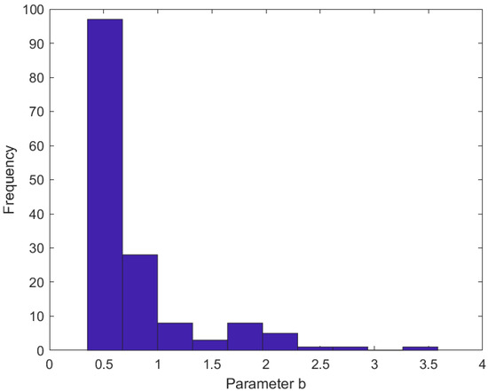
Figure 10.
Histogram plot of parameter ‘b’.
4.3. Model Performance in Rapidly Changing Atmospheric Systems
A key challenge in extreme weather forecasting is the ability of predictive models to handle highly dynamic and rapidly changing atmospheric conditions. While the proposed empirical model has demonstrated strong agreement with observed and simulated data under controlled scenarios, its applicability in fast-evolving climate systems remains an open question.
Extreme weather events, such as sudden pressure drops, heatwaves, and severe storms, often involve rapid fluctuations in key meteorological variables, making accurate prediction difficult. The empirical model relies on statistical parameters such as the integral time scale, mean, and standard deviation, which are derived from historical data. This approach ensures stability in long-term trends but may encounter limitations in situations where atmospheric conditions shift abruptly within short time frames.
To partially address this limitation, future work will focus on the dynamic calibration of the b parameter based on real-time meteorological inputs. By incorporating adaptive methods, such as rolling window analysis and machine learning-assisted parameter tuning, the model’s responsiveness to rapid changes could be significantly improved. Furthermore, expanding the dataset to include high-frequency measurements of pressure and temperature fluctuations during extreme weather events will provide additional insights into the model’s robustness.
Despite these challenges, the model’s efficiency and simplicity make it a valuable tool for extreme event forecasting, particularly in scenarios where computationally expensive simulations are impractical. A hybrid approach, combining empirical predictions with high-resolution numerical weather prediction (NWP) models, could further enhance predictive accuracy for highly dynamic climate conditions.
While the empirical model has been validated against high-fidelity LES data, its integration into CFD-RANS methodologies could provide a more computationally efficient framework for extreme value prediction. CFD-RANS simulations often struggle to accurately capture short-term peak fluctuations due to their inherent time-averaging approach. However, by incorporating the empirical model into existing RANS frameworks, the turbulence-induced maximum temperature and pressure fluctuations could be estimated more accurately without requiring costly LES simulations.
The empirical model could also complement NWP models, which rely on large-scale atmospheric data assimilation to forecast extreme events. The parameter b could be dynamically calibrated using real-time meteorological inputs, improving NWP forecasts by providing enhanced local-scale extreme value predictions. Future research should explore hybrid modeling approaches that integrate the empirical method with RANS-based turbulence closure models and machine-learning-assisted NWP predictions. Such an approach would enable faster and more accurate predictions of extreme atmospheric conditions in both urban and meteorological contexts.
Furthermore, one of the critical challenges in extreme weather forecasting is the ability of predictive models to handle rapidly evolving atmospheric conditions. While the proposed empirical model has demonstrated strong agreement with observed and simulated data under controlled scenarios, its applicability in highly dynamic environments requires further verification. Extreme weather events, such as sudden drops in pressure, heatwaves, or convective storms, often involve rapid fluctuations in key meteorological variables, posing challenges to traditional statistical approaches.
The empirical model relies on time-averaged statistical parameters such as the mean, standard deviation, and integral time scale, which are derived from historical data. This approach ensures stability in long-term trends but may encounter limitations in situations where atmospheric conditions change abruptly within short timeframes. Future studies should focus on evaluating the model’s predictive capabilities in fast-changing meteorological events by incorporating high-frequency, real-time datasets.
A potential improvement to the model’s adaptability in dynamic environments involves the real-time calibration of the b parameter. By continuously adjusting b based on incoming meteorological data, the model could better account for transient fluctuations in extreme conditions. This approach could be implemented through adaptive filtering techniques, such as Kalman filters, or by integrating short-term machine learning corrections to dynamically tune b. Additionally, testing the model across multiple extreme weather scenarios, including synoptic-scale disturbances, mesoscale convective systems, and rapid Arctic air mass intrusions, would provide further insights into its robustness.
To bridge the gap between empirical and numerical methods, a hybrid approach integrating the empirical model with high-resolution numerical weather prediction (NWP) models could be explored. For instance, the empirical model’s ability to estimate extreme values efficiently could be leveraged to refine ensemble weather forecasts, reducing computational costs while improving extreme event detection. Future research should aim to test these hybrid strategies in operational forecasting environments to assess their feasibility and accuracy.
4.4. Integration with Numerical Weather Prediction (NWP) Models
NWP models are widely used for forecasting extreme atmospheric conditions, leveraging large-scale atmospheric dynamics, real-time observations, and data assimilation techniques. While NWP models provide detailed spatiotemporal predictions, their computational cost and reliance on high-resolution input data can limit their applicability for rapid extreme value predictions. The empirical model proposed in this study offers a complementary approach by providing an efficient, statistically-driven method for estimating maximum atmospheric pressure and temperature, which can be integrated into NWP frameworks to enhance localized extreme event forecasts.
A key advantage of integrating the empirical model with NWP systems is its ability to refine extreme value predictions at sub-grid scales, where conventional NWP models often struggle with capturing peak fluctuations. The b parameter, which encapsulates application-specific uncertainties, can be dynamically adjusted based on real-time meteorological inputs from NWP forecasts. This adaptive approach would allow the empirical model to act as a correction mechanism, fine-tuning the maximum predicted values within the NWP framework.
Several integration strategies can be considered:
- Post-processing refinement: The empirical model can be used as a statistical post-processing tool to adjust NWP-predicted extreme values, similar to bias correction methods applied in ensemble forecasting.
- Hybrid modeling approach: By embedding the empirical model within NWP simulations, the model could provide real-time estimates of extreme values, improving the detection of sudden atmospheric fluctuations.
- Machine learning-assisted calibration: A data-driven approach could be explored where the b parameter is continuously updated using machine learning techniques, leveraging NWP forecasts and observational data for adaptive calibration.
Future research should focus on testing these integration strategies using high-resolution NWP outputs and real-time observational datasets. By incorporating the empirical model into operational NWP forecasting systems, it is possible to enhance the accuracy of extreme event predictions while reducing computational complexity, making it a viable tool for real-time atmospheric monitoring and early warning applications.
5. Discussion
This study introduced an empirical model for predicting extreme atmospheric conditions, focusing on maximum pressure and temperature fluctuations. The model integrates statistical parameters, including mean, standard deviation, integral time scale, and a correction factor b, which captures application-specific uncertainties. The results demonstrate the model’s adaptability across different atmospheric conditions, with b exhibiting significant variability depending on local climatic and geometric influences.
Despite its robust performance, several challenges remain. The b parameter introduces a degree of uncertainty, requiring further refinement to improve predictive accuracy. Additionally, while the model effectively captures extreme values in observational and simulated datasets, its applicability to rapidly evolving atmospheric systems still requires validation across a broader range of climatic conditions.
It should be noted that one of the key aspects in assessing the robustness of an empirical model is its ability to predict extreme values over different time scales. While the proposed model has been validated using high-frequency datasets, it has not yet been tested on time scales of 15–60 days, which are commonly used in sub-seasonal to seasonal (S2S) prediction frameworks. The lack of validation at these longer time scales is a recognized limitation of the current study. However, the model’s structure, which relies on statistical properties such as mean, standard deviation, and the integral time scale, suggests that it can be extended to capture variations in longer-term atmospheric trends. Future studies should focus on evaluating the model’s applicability for medium-range forecasting by incorporating datasets with extended temporal resolution. Such an approach could provide further insights into the model’s predictive capability for climate adaptation and decision-making processes.
5.1. Comparison with Machine Learning Approaches
In recent years, deep learning models such as convolutional neural networks (CNNs) and time series neural networks have demonstrated high accuracy in extreme weather prediction tasks. However, these models often require large training datasets, extensive computational resources, and careful hyperparameter tuning to achieve optimal performance. In contrast, the empirical model proposed in this study provides a computationally efficient alternative that is interpretable and directly incorporates statistical properties of atmospheric variability. Unlike machine learning approaches, which primarily rely on data-driven training, this empirical model integrates physically relevant statistical parameters such as the mean, standard deviation, integral time scale, and fluctuation intensity. The simplicity of the empirical approach makes it well-suited for rapid assessments and scenarios where high-quality training data for machine learning models may be limited [8]. Future research could explore potential hybrid approaches that leverage both methodologies, combining the interpretability of empirical models with the pattern recognition capabilities of deep learning.
5.2. Comparison with Traditional Physical Models
A key concern in extreme atmospheric condition modeling is the balance between computational efficiency and physical accuracy. Traditional NWP models and CFD methods, such as RANS and LES, offer physically grounded approaches by solving governing equations that describe atmospheric dynamics. However, these methods are often computationally expensive, especially when applied to extreme event prediction over large spatial and temporal scales.
In contrast, the empirical model proposed in this study provides an efficient alternative by leveraging statistical properties derived from observational and simulation data. Unlike RANS and LES, which require high-resolution turbulence modeling and extensive computational resources, the empirical model predicts extreme atmospheric conditions using statistical parameters such as mean values, standard deviations, and integral time scales. This approach allows for rapid estimation of maximum values without solving full Navier-Stokes equations.
Furthermore, while traditional NWP models utilize extensive data assimilation techniques to improve forecast accuracy, they often struggle with capturing localized extreme values due to their reliance on grid-based averaging techniques. The proposed empirical model complements these approaches by offering a low-computation method for refining extreme value predictions at finer spatial scales, particularly when combined with CFD-RANS methodologies.
Another advantage of the empirical model is its adaptability across multiple applications. Traditional physics-based models often require case-specific parameter tuning and boundary condition adjustments, which can limit their generalizability. The flexibility of the empirical model, particularly through the calibration of the b parameter, allows it to be applied across diverse atmospheric conditions with minimal computational cost.
Despite these advantages, it is important to acknowledge that the empirical model does not replace traditional physical models but rather complements them. The model provides an efficient means of estimating extreme atmospheric conditions, which can be further refined by integrating it with NWP or CFD frameworks. Future work should explore hybrid approaches that combine the empirical model’s rapid estimation capabilities with the detailed physics captured by numerical weather prediction and CFD-based methodologies.
5.3. Limitations and Future Directions
The empirical model presented in this study is built on statistical parameters that efficiently capture extreme atmospheric conditions. While causal discovery techniques could provide additional insights into the relationship between extreme weather events and large-scale climate drivers, their integration into the current framework is beyond the scope of this study. Causal discovery methods, such as Granger causality or structural equation modeling, require extensive datasets with well-defined causal structures, which are often unavailable for atmospheric extremes. Future research could explore the potential benefits of incorporating causal analysis into empirical modeling, particularly in contexts where climate dynamics and anthropogenic influences interact in a complex manner. However, the present study remains focused on providing a computationally efficient, interpretable, and generalizable empirical model for extreme value prediction.
Finally, future work should focus on:
- Refining the b parameter to minimize predictive variability and improve generalization across different environments.
- Extending validation to real-time forecasting applications and diverse meteorological datasets.
- Exploring hybrid approaches, integrating the empirical model with high-resolution numerical weather prediction (NWP) models.
- Enhancing interpretability, possibly through causal discovery techniques that connect extreme events to large-scale climate drivers.
6. Conclusions
This study presents an empirical model for predicting extreme atmospheric conditions, particularly maximum pressure and temperature. The model demonstrates strong agreement with observational and LES-derived data, highlighting its applicability to diverse meteorological scenarios. The study underscores the role of the b parameter in capturing local environmental variability, suggesting the need for further calibration efforts to enhance predictive accuracy. Future work will focus on expanding the dataset, refining parameter estimation methods, and integrating the empirical approach with numerical weather prediction (NWP) models for improved forecasting capabilities.
The model was validated using data from 29 global monitoring stations and LES results for an unstable boundary layer. The findings confirm that the model reliably estimates extreme values while maintaining computational efficiency.
Key takeaways from this study include:
- The empirical model demonstrated strong predictive capability for extreme pressure and temperature fluctuations.
- The b parameter played a crucial role in adapting predictions to specific environmental and geometric conditions.
- Model predictions aligned well with observed data, validating its applicability to extreme value forecasting.
While the model offers a computationally efficient alternative to traditional CFD-RANS approaches, further research is needed to refine the b parameter and enhance the model’s robustness under diverse atmospheric conditions. Future studies should focus on integrating the model with numerical weather prediction systems and expanding validation across various climatic settings.
Funding
This research received no external funding.
Institutional Review Board Statement
Not applicable.
Informed Consent Statement
Not applicable.
Data Availability Statement
Pressure data are freely available on the internet. Temperature data can be provided after communication with the scientists of the publication [13].
Acknowledgments
Efthimiou acknowledges the NMDB database www.nmdb.eu, (accessed on 1 January 2024), founded under the European Union’s FP7 programme (contract no. 213007) for providing the data. Also, Efthimiou would like to thank authors of the publication [13] for provide access to the temperature data.
Conflicts of Interest
The author declares no conflicts of interest.
References
- Melville, N.P. Information systems innovation for environmental sustainability. MIS Q. 2010, 34, 1–21. [Google Scholar]
- Lundstedt, H. Progress in space weather predictions and applications. Adv. Space Res. 2005, 36, 2516–2523. Available online: https://www.sciencedirect.com/science/article/pii/S0273117705000104 (accessed on 1 January 2025).
- Barlow, J.F. Progress in observing and modelling the urban boundary layer. Urban Clim. 2014, 10, 216–240. [Google Scholar] [CrossRef]
- Nazarian, N.; Fan, J.; Sin, T.; Norford, L.; Kleissl, J. Predicting outdoor thermal comfort in urban environments: A 3D numerical model for standard effective temperature. Urban Clim. 2017, 20, 251–267. [Google Scholar] [CrossRef]
- Bauer, P.; Thorpe, A.; Brunet, G. The quiet revolution of numerical weather prediction. Nature 2015, 525, 47–55. [Google Scholar] [CrossRef] [PubMed]
- Stensrud, D.J. Parameterization Schemes: Keys to Understanding Numerical Weather Prediction Models; Cambridge University Press: Cambridge, UK, 2007. [Google Scholar]
- Gentine, P.; Pritchard, M.; Rasp, S.; Reinaudi, G.; Yacalis, G. Could machine learning break the convection parameterization deadlock? Geophys. Res. Lett. 2018, 45, 5742–5751. [Google Scholar] [CrossRef]
- Rasp, S.; Pritchard, M.S.; Gentine, P. Deep learning to represent subgrid processes in climate models. Proc. Natl. Acad. Sci. USA 2018, 115, 9684–9689. [Google Scholar]
- Efthimiou, G. Application of an Empirical Model to Improve Maximum Value Predictions in CFD-RANS: Insights from Four Scientific Domains. Atmosphere 2024, 15, 1124. [Google Scholar] [CrossRef]
- Efthimiou, G.C.; Bartzis, J.G. Atmospheric dispersion and individual exposure of hazardous materials. J. Hazard. Mater. 2011, 188, 375–383. [Google Scholar] [PubMed]
- Bueno, B.; Roth, M.; Norford, L.; Li, R. Computationally efficient prediction of canopy level urban air temperature at the neighbourhood scale. Urban Clim. 2014, 9, 35–53. [Google Scholar] [CrossRef]
- Kambezidis, H.D.; Psiloglou, B.E.; Gavriil, A.; Petrinoli, K. Detection of Upper and Lower Planetary-Boundary Layer Curves and Estimation of Their Heights from Ceilometer Observations under All-Weather Conditions: Case of Athens, Greece. Remote Sens. 2021, 13, 2175. [Google Scholar] [CrossRef]
- Li, Y.; Wang, W.; Okaze, T. Evaluation of polyhedral mesh performance for large-eddy simulations of flow around an isolated building within an unstable boundary layer. Build. Environ. 2023, 235, 110207. [Google Scholar]
- Geleta, T.N.; Bitsuamlak, G. Validation metrics and turbulence frequency limits for LES-based wind load evaluation for low-rise buildings. J. Wind Eng. Ind. Aerod. 2022, 231, 105210. [Google Scholar] [CrossRef]
- Jiang, G.; Yoshie, R. Large-eddy simulation of flow and pollutant dispersion in a 3D urban street model located in an unstable boundary layer. Build. Environ. 2018, 142, 47–57. [Google Scholar] [CrossRef]
- Nazarian, N.; Krayenhoff, E.S.; Bechtel, B.; Hondula, D.M.; Paolini, R.; Vanos, J.; Cheung, T.; Chow, W.T.; de Dear, R.; Jay, O.; et al. Integrated assessment of urban overheating impacts on human life. Earth’s Future 2022, 10, e2022EF002682. [Google Scholar]
- Pereira, F.S.; Grinstein, F.F.; Israel, D.M.; Eça, L. Verification and validation: The path to predictive scale-resolving simulations of turbulence. J. Verif. Valid. Uncertain. Quantif. 2022, 7, 021003. [Google Scholar] [CrossRef]
- Lubchenco, J.; Karl, T.R. Predicting and managing extreme weather events. Phys. Today 2012, 65, 31–37. [Google Scholar] [CrossRef]
- Efthimiou, G.C.; Kumar, P.; Giannissi, S.G.; Feiz, A.A.; Andronopoulos, S. Prediction of the wind speed probabilities in the atmospheric surface layer. Renew. Energy 2019, 132, 921–930. [Google Scholar] [CrossRef]
- Bartzis, J.G.; Sfetsos, A.; Andronopoulos, S. On the individual exposure from airborne hazardous releases: The effect of atmospheric turbulence. J. Hazard. Mater. 2008, 150, 76–82. [Google Scholar] [CrossRef] [PubMed]
- Wilks, D.S. Statistical Methods in the Atmospheric Sciences; Academic Press: Cambridge, MA, USA, 2011. [Google Scholar]
- Yoshie, R.; Jiang, G.; Shirasawa, T.; Chung, J. CFD simulations of gas dispersion around high-rise buildings in non-isothermal boundary layer. J. Wind. Eng. Ind. Aerodyn. 2011, 99, 279–288. [Google Scholar] [CrossRef]
Disclaimer/Publisher’s Note: The statements, opinions and data contained in all publications are solely those of the individual author(s) and contributor(s) and not of MDPI and/or the editor(s). MDPI and/or the editor(s) disclaim responsibility for any injury to people or property resulting from any ideas, methods, instructions or products referred to in the content. |
© 2025 by the author. Licensee MDPI, Basel, Switzerland. This article is an open access article distributed under the terms and conditions of the Creative Commons Attribution (CC BY) license (https://creativecommons.org/licenses/by/4.0/).