Article

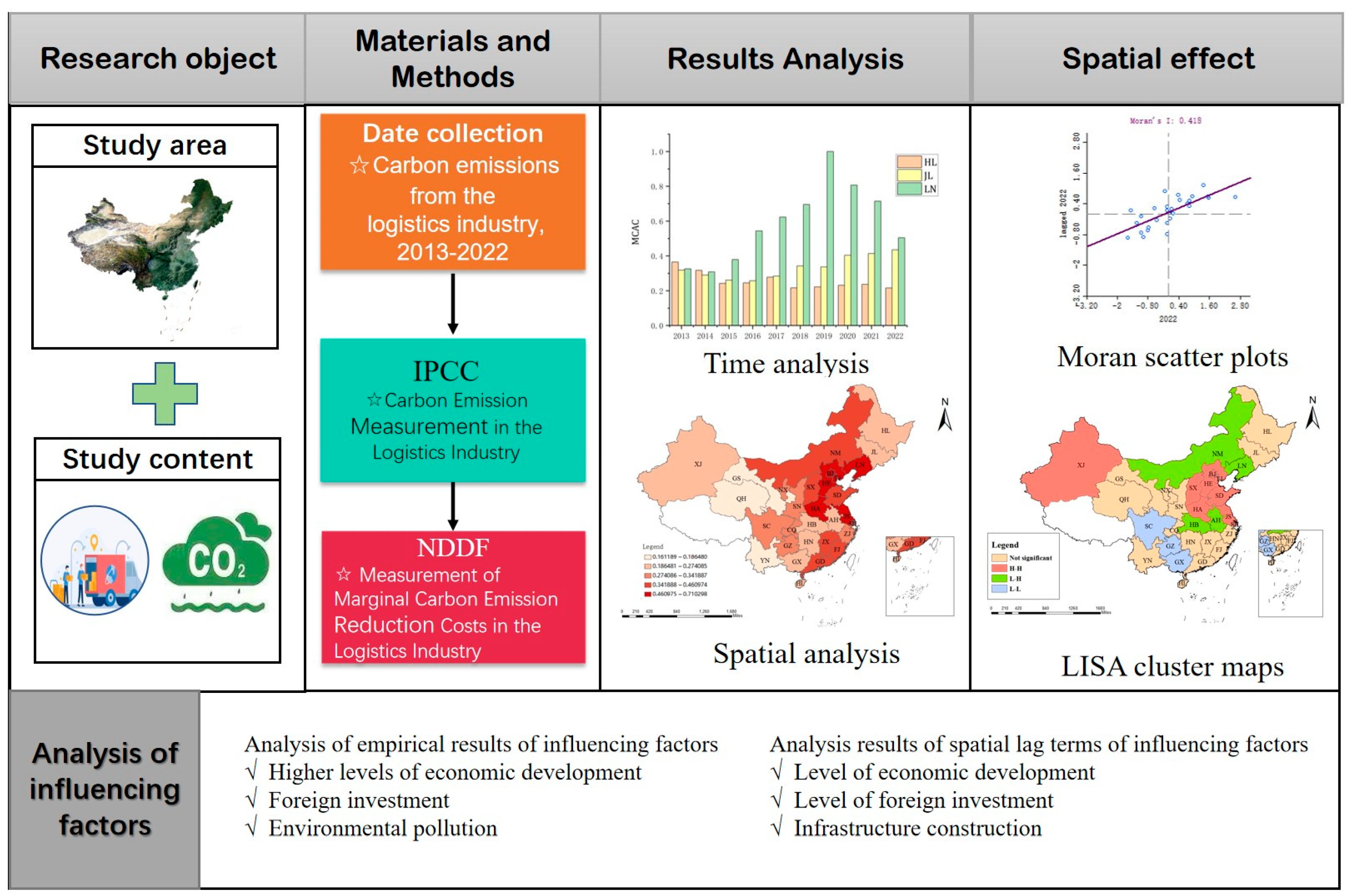
Research on the Temporal and Spatial Distribution of Marginal Abatement Costs of Carbon Emissions in the Logistics Industry and Its Influencing Factors

Research Center of Energy Economic, School of Business Administration, Henan Polytechnic University, Jiaozuo 454003, China
*
Author to whom correspondence should be addressed.
Sustainability 2025, 17(7), 2839; https://doi.org/10.3390/su17072839
Submission received: 18 February 2025 / Revised: 14 March 2025 / Accepted: 20 March 2025 / Published: 22 March 2025
(This article belongs to the Collection Air Pollution Control and Sustainable Development)

Abstract

:
While existing research has focused on logistics carbon emissions, understanding spatiotemporal emission cost dynamics and drivers remains limited. This study bridges three gaps through methodological advances: (1) Applying the Non-Radial Directional Distance Function (NDDF) to measure Marginal Carbon Abatement Costs (MCAC), overcoming traditional Data Envelopment Analysis (DEA) model’s proportional adjustment constraints for provincial heterogeneity; (2) Pioneering dual-dimensional MCAC analysis integrating temporal trends (2013–2022) with spatial autocorrelation; and (3) Developing a spatial Durbin error model with time-fixed effects capturing direct/indirect impacts of innovation and infrastructure. Based on provincial data from 2013–2022, our findings demonstrate a U-shaped temporal trajectory of MCAC with the index fluctuating between 0.3483 and 0.4655, alongside significant spatial heterogeneity following an Eastern > Central > Northeastern > Western pattern. The identification of persistent high-high/low-low clusters through local Moran’s I analysis provides new evidence of spatial dependence in emission reduction costs, with these polarized clusters consistently comprising 70% of Chinese cities throughout the study period. Notably, the spatial econometric results reveal that foreign investment and logistics infrastructure exert competitive spillover effects, paradoxically increasing neighboring regions’ MCAC, a previously undocumented phenomenon in sustainability literature. These methodological advancements and empirical insights establish a novel framework for spatial cost allocation in emission reduction planning.

1. Introduction

As the lifeblood of national economic development, the logistics industry, while supporting rapid economic growth, is increasingly challenged by energy consumption and carbon emissions [1]. In 2023, the total value of social logistics in China reached RMB 352.4 trillion, representing a year-on-year increase of 5.2%. However, the industry’s expansion, coupled with its reliance on fossil fuels, has led to a persistent increase in carbon emissions [2]. Transportation, warehousing, and postal services account for 85% of the industry’s total output value, and their high energy consumption characteristics make the logistics industry a key sector for achieving the “dual carbon” goals [3]. In this context, balancing logistics revenue and the marginal cost of abatement (MCAC) has become a pressing challenge that needs to be addressed.
MCAC, as a core indicator for measuring the opportunity cost of emission reductions, provides a quantitative basis for developing low-carbon policies. Existing research has mostly focused on industries [4], urban agglomerations [5,6], and carbon trading systems [7], with insufficient attention has been paid to the spatiotemporal characteristics and spatial spillover effects of MCAC in the logistics industry. Notably, logistics networks have inherent cross-regional interconnectivity, and their carbon emissions may exhibit significant spatial dependence [8]. Ignoring this characteristic may lead to biases in emission reduction cost estimates, thereby affecting the accuracy of policy design.
This paper aims to fill the following research gaps: First, it adopts the non-radial directional distance function (NDDF) to optimize MCAC measurement in the logistics industry, addressing efficiency overestimation in traditional radial models. Second, it reveals the spatiotemporal differentiation patterns and spatial spillover mechanisms of MCAC in the logistics industry through spatial autocorrelation analysis and econometric models. Third, it identifies key driving factors to provide a basis for differentiated emission reduction strategies. The research findings can provide theoretical support for carbon tax pricing, the design of cross-regional emission trading systems, and offer methodological references for studies on emission-reduction costs in other industries.
The rest of this paper is structured as follows. Section 1 provides an introduction to the research background and significance of studying the marginal abatement costs of carbon emissions in the logistics industry. Section 2 conducts a systematic literature review, focusing on MCAC measurement methods, spatial effects of carbon reduction costs, and key influencing factors. In Section 3, the research methodology and data sources are elaborated. Section 4 presents the empirical results and analysis. Section 5 discusses the policy implications of the findings, emphasizing the necessity of spatial spillover effects in cross-regional carbon governance. Section 6 proposes targeted recommendations for optimizing emission reduction strategies in the logistics sector, such as promoting multimodal transport and enhancing green technology diffusion. The specific research framework is shown in Figure 1.

2. Literature Review

2.1. Evolution of MCAC Measurement Methods

MCAC estimation primarily relies on the theory of shadow prices, with the core focus being the determination of the marginal rate of substitution for emission reductions through the production frontier. Early studies mostly used parametric stochastic frontier analysis (SFA), but the need to preset functional forms led to potential model misspecification [9]. Non-parametric data envelopment analysis (DEA) has been widely adopted due to its advantage of not requiring a priori production functions. For example, Wu et al. measured provincial MCAC in China by improving the directional distance function [10]. Cristea et al. used DEA to measure the shadow price of undesirable outputs, finding that countries at different levels of development are comparable in terms of their economic and environmental performance [11]. However, traditional radial models require proportional adjustments to inputs and outputs, making it difficult to reflect asymmetric efficiency losses in reality. For this purpose, the NDDF introduces a flexible direction vector [12], which allows for heterogeneous adjustments to inputs and outputs, making it more suitable for multi-factor collaborative optimization scenarios, including logistics transportation and warehousing. For example, Choi et al. applied the NDDF to evaluate the environmental performance of the freight sector with respect to PM2.5 and NOx air pollution across 16 local governments in Korea, thereby confirming the method’s effectiveness in complex application contexts [13]. Therefore, this paper adopts the NDDF framework to more accurately capture the heterogeneity of carbon abatement technologies in logistics transportation, warehousing, and related areas.

2.2. Spatial Effects of Carbon Reduction Costs

The spatial correlation of carbon emissions has been confirmed by empirical studies in multiple fields. At the industry level, Tang et al., using a multi-regional input-output model, found that carbon emissions have direct, indirect, and spatial feedback effects [14]. Du Q et al. revealed that the spatial spillover of carbon efficiency in the construction industry exhibits positive agglomeration characteristics [15]. Wahab et al., based on the impact of consumption-based carbon emissions, employed a time-space fixed model and found that renewable energy has a positive spillover effect, while economic growth and bilateral exports have a negative impact on consumption-based carbon emissions [16]. For the logistics industry, its networked operation mode strengthens the spatial dependence of inter-provincial carbon emissions: cross-regional freight transportation lines lead to emission transfers, and the diffusion of low-carbon technologies in hub cities may generate spillover benefits [8]. However, existing literature mostly focuses on the spatial effects of industrial carbon emissions [17] and lacks an in-depth analysis of the spatial spillover paths of MCAC in the logistics industry.

2.3. Research on MCAC Influencing Factors

Existing studies have shown that emission reduction costs are influenced by multidimensional factors such as energy intensity, industrial structure, and policy regulation. At the macro level, energy consumption intensity has been proven to be negatively correlated with MCAC [6], while an increase in the proportion of the tertiary industry can reduce emission reduction costs through technology diffusion [7]. Micro-level enterprise data indicate that the impact of environmental regulations on MCAC is heterogeneous: strict policies drive technological innovation but may increase compliance costs in the short term [18]. In the logistics industry, however, additional unique factors come into play. For instance, regional economic levels can play a significant role in reducing unit emission costs by providing the necessary infrastructure and resources [19]. Despite these distinctive characteristics, current research has not yet systematically integrated these logistics-specific factors into the analysis of MCAC, leaving a gap in our understanding of the complete influence paths within this sector.

2.4. Research Gaps and This Paper’s Positioning

Although research on MCAC in other sectors has achieved fruitful results, there are three limitations in the field of logistics. First, measurement methods predominantly follow industrial models, which overlook the unique characteristics of MCAC in logistics operations. Second, spatial effect analyses have focused on total emissions [20], failing to identify the spatial spillover mechanisms of emission reduction costs. Third, studies on influencing factors have emphasized macro indicators without thoroughly examining industry-specific variables. This paper advances research in this field by constructing an NDDF model specifically tailored for the logistics industry and integrating a Spatial Durbin Model (SDM) to analyze inter-provincial spillover effects.
In summary, existing studies have provided valuable insights into the estimation methods, spatial effects, and influencing factors of MCAC across various industries. However, research specifically focusing on the logistics sector remains limited. While many studies have employed parametric and non-parametric approaches to estimate MCAC, the unique characteristics of logistics operations are often overlooked. Additionally, although spatial spillover effects have been widely examined in industrial carbon emissions, there is a lack of in-depth exploration into how these effects influence carbon abatement costs in logistics. Moreover, previous research has primarily emphasized macroeconomic indicators, with limited attention given to industry-specific determinants like logistics specialization and network density. Addressing these gaps, this study constructs an NDDF model tailored to the logistics sector, integrates spatial econometric methods to analyze spillover effects, and incorporates key industry-specific variables to provide a more comprehensive understanding of MCAC in logistics.

3. Materials and Methods

3.1. Research Methods

3.1.1. Carbon Emission Measurement in the Logistics Industry

Currently, three primary methods are employed to assess carbon emissions in the logistics sector: the IPCC direct energy consumption coefficient approach, the indirect input-output model, and the comprehensive energy consumption lifecycle analysis [21,22,23]. Research indicates that the combustion of fossil fuels accounts for 95% of the carbon emissions released into the atmosphere. By aggregating emissions from various energy sources, it is possible to calculate the total carbon output of a particular region or sector, providing an indication of its overall emission levels. Building on previous studies [24,25,26,27,28], this research identifies fossil fuel emissions as the key indicator of atmospheric carbon levels.
The formula for estimating carbon emissions is defined as:
C = j C j = j f j × h j × e j
Here, C denotes the aggregate carbon dioxide emissions generated by the logistics sector, while j signifies the different categories of energy sources. f j is the emission coefficient for energy type j , as shown in Table 1. h j denotes the standard coal conversion factor. e j signifies the total consumption of energy type j , as shown in Table 2.

3.1.2. Measurement of MCAC in the Logistics Industry

The NDDF in DEA addresses the limitations of traditional approaches by considering varying trends involving both valuable and adverse outputs. As a relatively novel methodology for calculating MCAC, the NDDF resolves deficiencies in conventional radial algorithms through its capacity to accommodate differential change patterns between desirable outputs and undesirable outputs [29]. This model involves fewer theoretical assumptions and enhances the comparability of individual economic performance across sectors and mitigation scenarios [30,31]. By explicitly quantifying inter-sectoral disparities in abatement costs, it enables precise measurement of economic pressures on specific industries and comparative evaluation of emission allocation schemes’ cost-effectiveness. Consequently, this research employs the NDDF approach to estimate the MCAC within the logistics industry.
Recent research suggests that input indicators typically consist of variables such as capital stock, workforce, and energy usage [32,33,34,35]. Specifically, this research considers fixed asset investment, employment, and energy use within the logistics sector as input variables. The logistics sector’s GDP is treated as the desirable output, while CO2 emissions are classified as the undesirable output [23,36,37].
Drawing on the work of Dai and Kuosmanen [38] and Zhou et al. [12], this study employs the NDDF method, utilizing Kuosmanen’s approach, to estimate the value of a particular decision-making unit, represented as D M U o , denoted as N D K , L , E , Y , Q ; g :
N D K , L , E , Y , Q ; g = max ω k β k + ω L β L + ω E β E + ω Y β Y + ω Q β Q s . t . i = 1 N Z i K i K 0 + β K g K i = 1 N Z i L i L 0 + β L g L i = 1 N Z i E i E 0 + β E g E i = 1 N θ i Z i Y i Y 0 + β Y g Y i = 1 N θ i Z i Q i = Q 0 + β Q g Q i = 1 N Z i = 1 Z i 0 , i = 1 , , N 0 θ i 1 , i = 1 , , N
where ω T = ω K , ω L , ω E , ω Y , ω Q represents the standardized weight vector assigned to both inputs and outputs. Z i represents the intensity variables, which are utilized to scale individual inputs and outputs either by expansion or contraction. The multiplier θ i signifies the individual emission reduction factor; g = g K , g L , g E , g Y , g Q is the direction vector.
Based on the current research by scholars, this paper sets the weight vector ω T = 1 9 , 1 9 , 1 9 , 1 3 , 1 3 and the direction vector g = K , L , E , Y , B . Let λ i = θ i Z i , μ i = 1 θ i Z i , Equation (2) can be transformed into
N D K , L , E , Y , Q ; g = max ω K β K + ω L β L + ω E β E + ω Y β Y + ω Q β Q s . t . i = 1 N λ i + μ i K i K 0 + β K g K i = 1 N λ i + μ i L i L 0 + β L g L i = 1 N λ i + μ i E i E 0 + β E g E i = 1 N λ i Y i Y 0 + β Y g Y i = 1 N λ i Q i Q 0 + β Q g Q i = 1 N λ i + μ i = 1 λ i , μ i 0 , i = 1 , , N 0 θ i 1 , i = 1 , , N
Since MAC is defined as the ratio between the shadow price of carbon emissions and economic output, this study develops a dual model to determine the solution. The formulation of the dual model is as follows:
N D K , L , E , Y , Q ; g = min μ K i K i + μ L i L i + μ E i E i + μ Y i Y i + μ Q i Q i + ϕ i s . t . i = 1 N μ K i K i + μ L i L i + μ E i E i + μ Y i Y i + μ Q i Q i + ϕ i 0 i = 1 N μ K i K i + μ L i L i + μ E i E i + ϕ i 0 μ K i K i 1 ; μ L i L i 1 ; μ E i E i 1 ; μ Y i Y i 1 ; μ Q i Q i 1 μ K i 0 ; μ L i 0 ; μ E i 0 ; μ Y i 0 ;
where ϕ i , μ K i , μ L i , μ E i , μ Y i , μ Q i are all dual variables. ϕ i represents the returns to scale for D M U i . MAC can be expressed as
M A C i = ρ Y i μ Q i μ Y i
where ρ Y i denotes the absolute shadow price of the desired output, which, by definition, is assigned a value of 1 yuan per ton. M A C i is the MAC for sub-sector i i.

3.1.3. Spatial Analysis Method for MCAC in the Logistics Industry

This research utilizes spatial autocorrelation analysis to analyze the geographic patterns of MCAC within the logistics industry. Spatial autocorrelation analysis focuses on investigating data with spatial variability, where the value of a given variable is influenced by the corresponding values in neighboring regions [39,40]. This study analyzes the MCAC of the logistics industry across 30 provinces and municipalities within China. Each province and city exhibits spatial influence and spatial dimensionality in logistics production activities, referred to in spatial econometrics as spatial dependence and spatial heterogeneity.
(1)
Spatial Dependence. Spatial dependence refers to the interdependence and mutual influence of a phenomenon across different spatial units [41,42]. It signifies the consistency between the target value and the region, also known as spatial autocorrelation. The intensity of spatial correlation is influenced by both absolute and relative positions. The methods used for its measurement involve both overall and regional autocorrelation. The Moran’s I statistic is commonly employed to assess overall autocorrelation, which examines the overall spatial distribution characteristics of a particular phenomenon. Local autocorrelation focuses on the clustered patterns of a phenomenon within local spaces, often represented by Moran’s I scatter plots and LISA maps.
(2)
Spatial Heterogeneity. Spatial heterogeneity refers to the differences in a phenomenon between different spatial units, such as the disparities between China’s eastern coastal and western regions or between economically developed and underdeveloped areas. These differences are caused by the uneven and non-random distribution of the spatial economy [43]. In this study, spatial heterogeneity is primarily driven by variations in energy consumption, economic inputs, and labor force distribution across different regions within the logistics industry.
(3)
Moran’s I Index. Moran’s I is a method used to assess spatial autocorrelation, taking into account the intricate nature of spatial sequences in its calculations [44]. The associated formula is given below:
I = i = 1 n j = 1 n w i j x i x ¯ x j x ¯ s 2 i = 1 n j = 1 n w i j
where S 2 = 1 n i = 1 n x i x ¯ 2 represents the variance of the research data. w i j is the i , j element of the spatial weight matrix, which indicates the distance between i and j . i = 1 n j = 1 n w i j represents the sum of the spatial weights of all research objects. If the spatial weight matrix is row-standardized, then i = 1 n j = 1 n w i j = n . In this case, Moran’s I can be written as
I = i = 1 n j = 1 n w i j x i x ¯ x j x ¯ i = 1 n x i x ¯ 2
Moran’s I ranges from −1 to 1. A value above 0 indicates positive spatial correlation, meaning nearby regions have similar characteristics. A value below 0 shows negative spatial correlation, where high-value regions are often surrounded by low-value areas and vice versa. If Moran’s I is close to 0, it suggests little to no spatial autocorrelation.
To determine whether a significant spatial correlation exists in the logistics MCAC across n regions, the standardized statistic Z can be used. The formula is provided below:
Z = M o r a n s   I E I V A R I
where E I = 1 n 1 , V A R I = n 2 w 1 + n w 2 + 3 w 0 2 w 0 2 n 2 1 E 2 I , w 0 = i = 1 n j = 1 n w i j , w 1 = 1 2 i = 1 n j = 1 n w i j + w j i 2 , w 2 = i = 1 n w i + w j 2 . Where w i and w j represent the sum of the i row and j column of the spatial weight matrix, respectively.
(4)
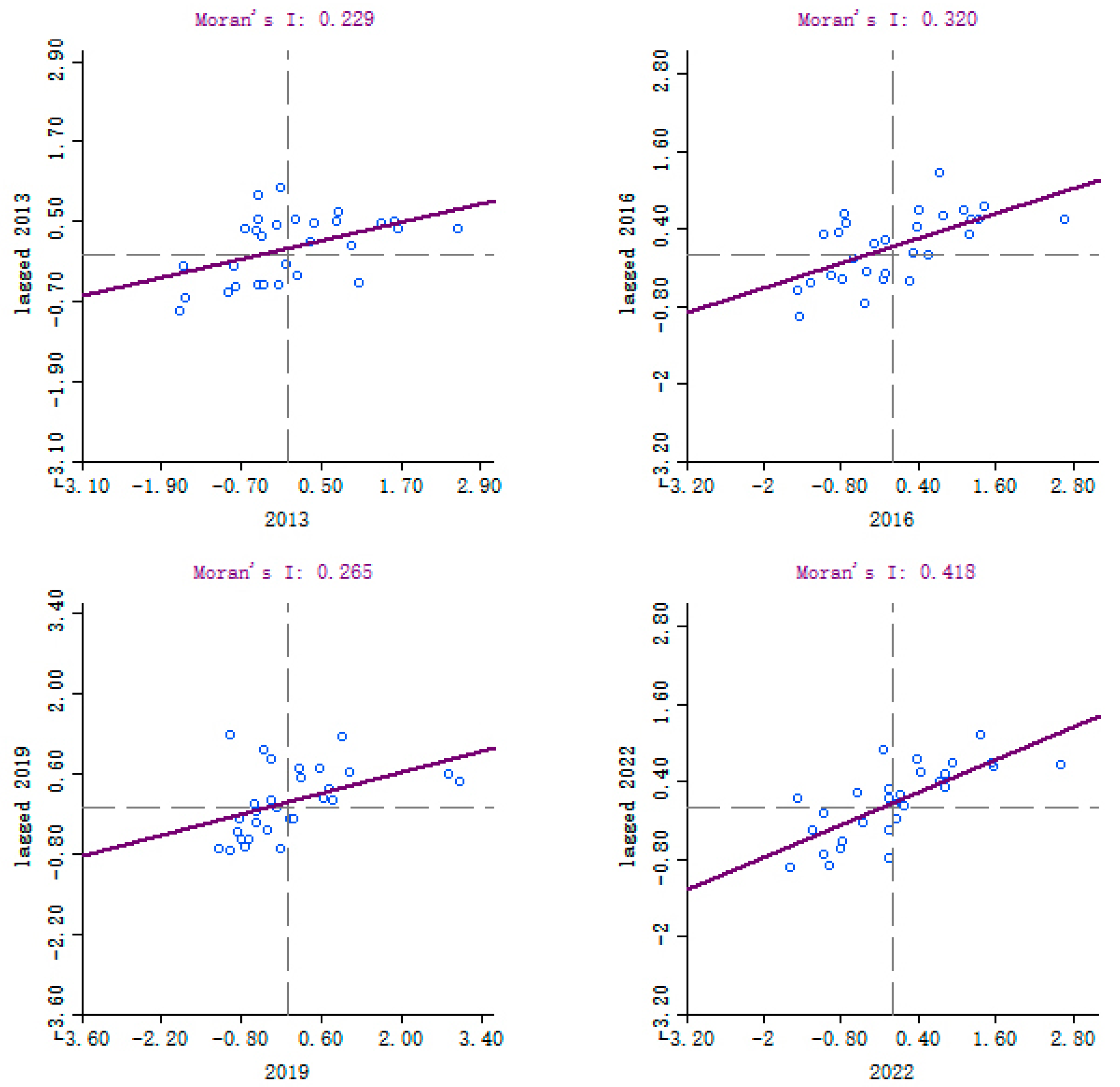
Moran’s scatter plot is used to analyze spatial patterns within localized areas. This approach presents the data using a scatter plot, with the vertical axis depicting spatial lag values and the horizontal axis displaying deviation values for each region, effectively highlighting spatial lag influences [45]. The scatter plot consists of four quadrants, each representing a unique local spatial relationship. The first and third quadrants indicate positive spatial correlations, suggesting that the target region and its surrounding areas exhibit comparable levels. In contrast, the second and fourth quadrants reveal negative spatial correlations, reflecting differences in development levels between the target region and its surroundings. A detailed explanation is available in Table 3.
(5)
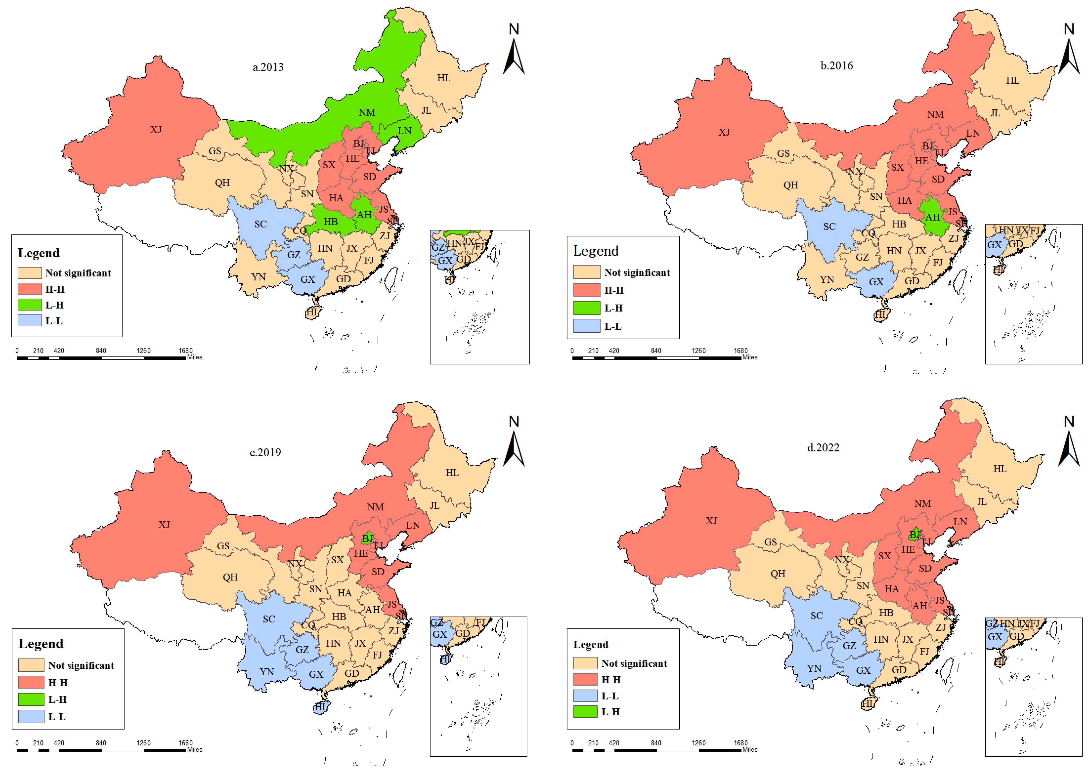
LISA Cluster Map. While Moran’s scatter plot provides an intuitive view of the relationships between each target region and its surrounding areas, it does not clearly indicate the significance of spatial correlation in that region [46,47]. The LISA cluster map, however, not only visually displays the significance of spatial clustering around each region but also highlights the spatial units and patterns that influence the overall spatial distribution. By computing the local Moran’s I index and utilizing software packages such as StataMP 17 and ArcGIS 10.8, one can generate a LISA cluster map that illustrates the MCAC in China’s logistics industry.
I i = x i x ¯ j = 1 n w i j x j x ¯ S 2
In the aforementioned formula, I i represents the value of the local Moran’s I index. s 2 = i = 1 n x i x ¯ 2 n denotes the variance of the studied data, and w i j is the i , j element of the spatial weight matrix, signifying the distance between i and j .
A positive value of the local Moran’s I index indicates that the target area and its surrounding regions exhibit similar characteristics or patterns. Conversely, a negative value suggests differences between the target region and its surrounding areas. By conducting significance tests on the local Moran’s I index, spatial clusters are identified, enabling creation of a LISA cluster map. This map visually highlights the significance of MCAC in logistics industry across 30 provinces in China.

3.1.4. Construction of Spatial Econometric Model

The temporal and spatial distribution of MCAC in China’s logistics sector may exhibit a degree of spatial correlation. Traditional regression analysis methods may not adequately explain such phenomena, while spatial econometric models incorporate spatiotemporal correlations to some extent. For this reason, this paper employs a spatial econometric model for analyzing the driving factors. To assess the relationship between the dependent variable and its influencing factors, a linear model is initially adopted before exploring other potential methods. Typically, the Ordinary Least Squares (OLS) regression model is used [48,49], and its formula is
m i n F ( x ) = i = 1 m ( y i w x i b ) 2
where y i represents the marginal abatement cost in the logistics industry, x i represents the value of the influencing factor, b is the constant term, and w is the coefficient. To calculate the coefficients in the above formula, by taking the derivative of F x with respect to w and b , we can obtain
E ( w , b ) w = 2 ( w i = 1 m x i 2 i = 1 m ( y i b ) x i ) E ( w , b ) b = 2 m b i = 1 m y i w x i
By equating the partial derivatives to 0, we can determine the specific values of the coefficients. Here is the specific formula:
w = i = 1 m y i ( x i x ¯ ) i = 1 m x i 2 1 m ( i = 1 m x i ) 2 b = 1 m i = 1 m y i w x i
where x ¯ = 1 m i = 1 m x i . In the 1970s, the spatial econometric model was proposed, which fully considers the relationship between space and regional economy. The formula for the spatial econometric model is
y i t = ρ j = 1 N w i j y j t + φ + X i t β + j = 1 N w i j X i j t γ + μ i + η t + ϕ i t ϕ i t = λ j = 1 N w i j ϕ i t + ε i t
In the above formula, y i t represents the dependent variable at time t in the i region ( i = 1 , 2 , 3 , , N ; t = 1 , 2 , 3 , , T ) . w i j is the spatial weight matrix for N × N . j = 1 N w i j y j t represents the impact that the dependent variables in adjacent regions have on the current region. ρ represents the coefficient of the spatial autoregression of the dependent variable. X i t is a K -dimensional explanatory variable. β is a K × 1 -dimensional vector of parameter estimation coefficients for the regression component. j = 1 N w i j X i j t γ represents the influence of the independent variables in neighboring regions on the independent variables in the current region. γ is an K × 1 -dimensional spatial autocorrelation coefficient matrix. μ i is the spatial effect term, η t is the time effect term, ϕ i t is the error term, λ is the spatial autocorrelation coefficient of the error term, and ε i t is the independently and identically distributed error term ε i t N 0 , σ 2 .
Spatial econometric models have continually evolved, branching into various submodels such as the Spatial Autoregressive Model (SAR), Spatial Error Model (SEM), and Spatial Durbin Model (SDM), among others. The Spatial Autoregressive Model examines indicators with significant spatial dependence, where nearby changes affect local values through spatial interactions. The Spatial Error Model focuses on variations arising from differing locations, while the Spatial Durbin Model addresses environments. In this context, the local dependent variable is influenced by both its own explanatory factors and the dependent variables from neighboring regions. By imposing certain constraints, the formulae for these models can be formulated.
Spatial Autoregressive Model λ = γ = 0 :
y i t = ρ j = 1 N w i j y j t + φ + X i t β + μ i + η t + ϕ i t
Spatial Error Model (SEM) ρ = γ = 0 :
y i t = φ + X i t β + μ i + η t + ϕ i t ϕ i t = λ j = 1 N w i j ϕ i t + ε i t
Spatial Durbin Model (SDM) λ = 0
y i t = ρ j = 1 N w i j y j t + φ + X i t β + j = 1 N w i j X i j t γ + μ i + η t + ε i t

3.1.5. Selection of Influencing Factors

For the selection of influencing factor indicators for the MCAC in the logistics industry, MCAC is taken as the dependent variable. Economic development level, education investment level, innovation development level, foreign investment level, environmental pollution, and infrastructure construction are considered as explanatory variables. Based on these, a spatial econometric model is constructed for the marginal emission reduction cost of China’s logistics industry. The final selected indicators for the influencing factors of the marginal abatement cost within logistics are shown in Table 4.

3.2. Data Sources

This study selects panel data from 30 provinces in China spanning from 2013 to 2022. The selection of this time period is based on the following considerations: Firstly, the State Council issued the Action Plan for Air Pollution Prevention and Control in 2013, marking the entry of environmental regulation policies into a systematic phase. Secondly, the standardization of provincial energy consumption statistics after 2013 ensures data consistency. Thirdly, this time period covers the critical transition from the 13th Five-Year Plan to the 14th Five-Year Plan, allowing for the observation of the dynamic impact of dual carbon goals on the logistics industry. The study area is 30 provinces and municipalities in China, excluding some with missing data, such as Hong Kong, Macao, Taiwan, and Tibet. This study divides China into four regions: Eastern, Central, Western, and Northeastern, with each region comprising the provinces and municipalities, as shown in Table 5. In subsequent research, the provinces and municipalities will be referred to using their abbreviations. Due to the absence of a distinct classification for the logistics sector in China, the transport, storage, and postal services industry is adopted as a proxy, consistent with prior studies. Data is sourced from multiple editions of the China Statistical Yearbook, China Science Statistical Yearbook, and so on.

4. Results Analysis

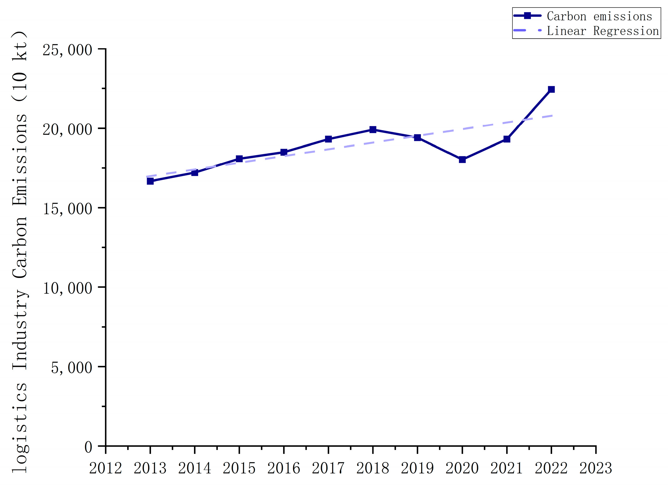
4.1. Analysis of Carbon Emission Estimation Results for the Logistics Industry in Various Regions

By applying a suitable formula for carbon emission calculations and utilizing relevant datasets, the carbon emissions generated by China’s logistics sector were assessed for the years 2013 to 2022. The results are presented in Table 6, along with a line chart illustrating the national logistics industry’s carbon emissions based on the computed data and a linear regression analysis of the growth trend shown in Figure 2, “Carbon emissions of China’s logistics industry from 2013 to 2022 and linear fit”.
The decline observed between 2019 and 2020 was primarily caused by the external disruption of COVID-19, which affected logistics transportation and personnel, resulting in decreased emissions. Despite this temporary reduction, the linear regression analysis confirms an upward trajectory in emissions. With continuous technological advancements and improvements in logistics infrastructure, it is projected that carbon emissions in the logistics sector will continue to rise.

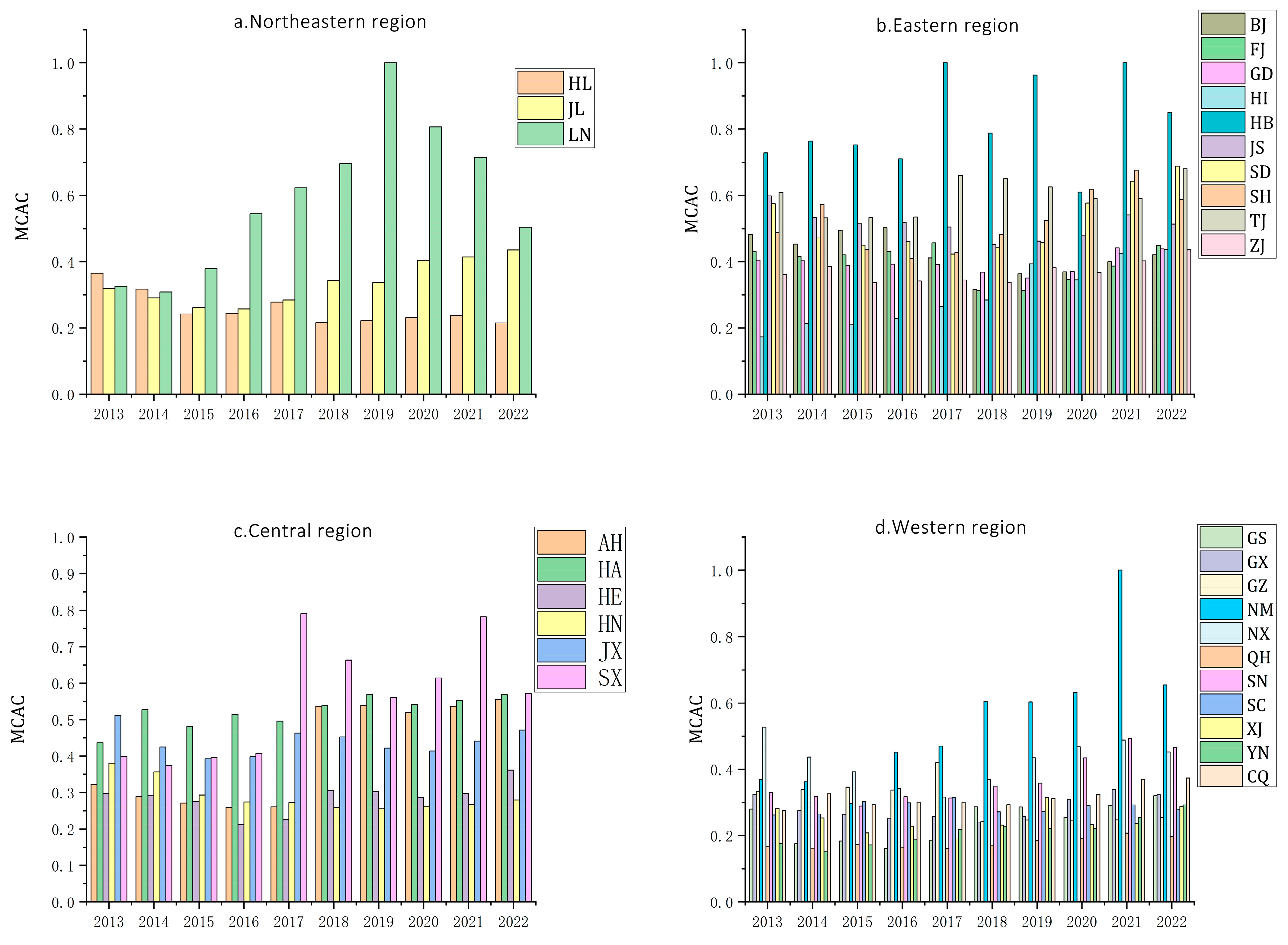
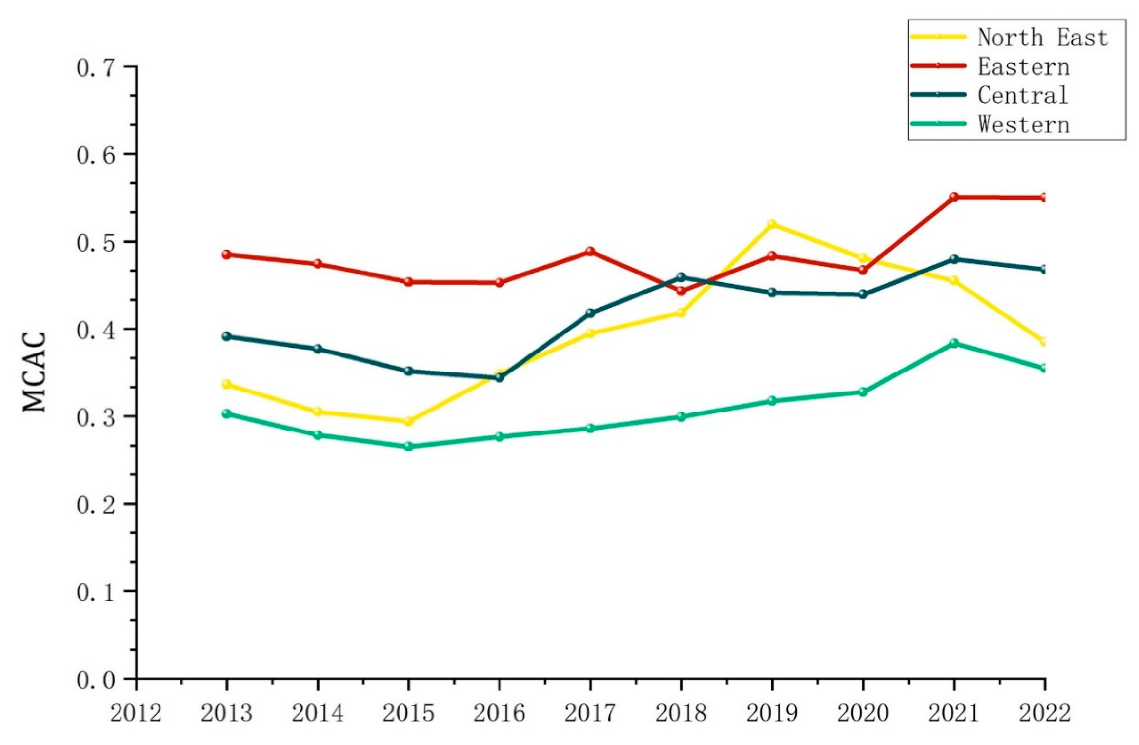
4.2. Analysis of MCAC Calculation Results in the Logistics Industry

Using the previously mentioned model, the MCAC for the logistics industry was calculated, and the results are detailed in Table 7.
The table highlights significant variations in the MCAC of the logistics sector across different provinces and cities, reflecting diverse trends and cost disparities. At the national level, the MCAC for the logistics industry decreased between 2013 and 2015, after which it experienced an overall increase from 2015 to 2022. The lowest recorded value was 0.3483 in 2015, while the highest reached 0.4655 in 2021.

4.2.1. Temporal Dimension Analysis of MCAC in the Logistics Industry

Drawing on the computed MCAC values for the logistics sector across 30 provinces and cities in China, this study examines the regional trends in MCAC from 2013 to 2022. The analysis categorizes the data into four major regions—Northeast, East, Central, and West—to highlight variations in different parts of the country.
Figure 3 displays the MCAC and its trends for the logistics industry within China’s four major regions from 2013 to 2022. The Northeast region has exhibited a general pattern of growth followed by decline, with MCAC increasing from 0.4831 million yuan per ton in 2013 to a peak of 0.5195 million yuan per ton in 2019 before dropping to 0.3848 million yuan per ton by 2022. The Eastern and Western regions have shown a consistent upward trend overall, while the Central region has experienced noticeable variations. The factors influencing the fluctuations in the MCAC of the logistics industry across different regions in China lie in the country’s emphasis on sustainable development and green transformation. Logistics companies are in a phase of adaptation, undergoing transformation and upgrading as they align with sustainability goals and evolving policies, which subsequently impacts the changes in MCAC.
As shown in Figure 4, the MCAC for the logistics industry is generally higher in the Northeast, East, and Central regions compared to the West. Calculations reveal that the annual average marginal abatement cost stands at 0.3937 million yuan/ton in the Northeast, 0.4848 million yuan/ton in the East, 0.4169 million yuan/ton in the Central region, and 0.3092 million yuan/ton in the West. This demonstrates a pattern of West < Northeast < Central < East.

4.2.2. Spatial Dimension Analysis of MCAC in the Logistics Industry
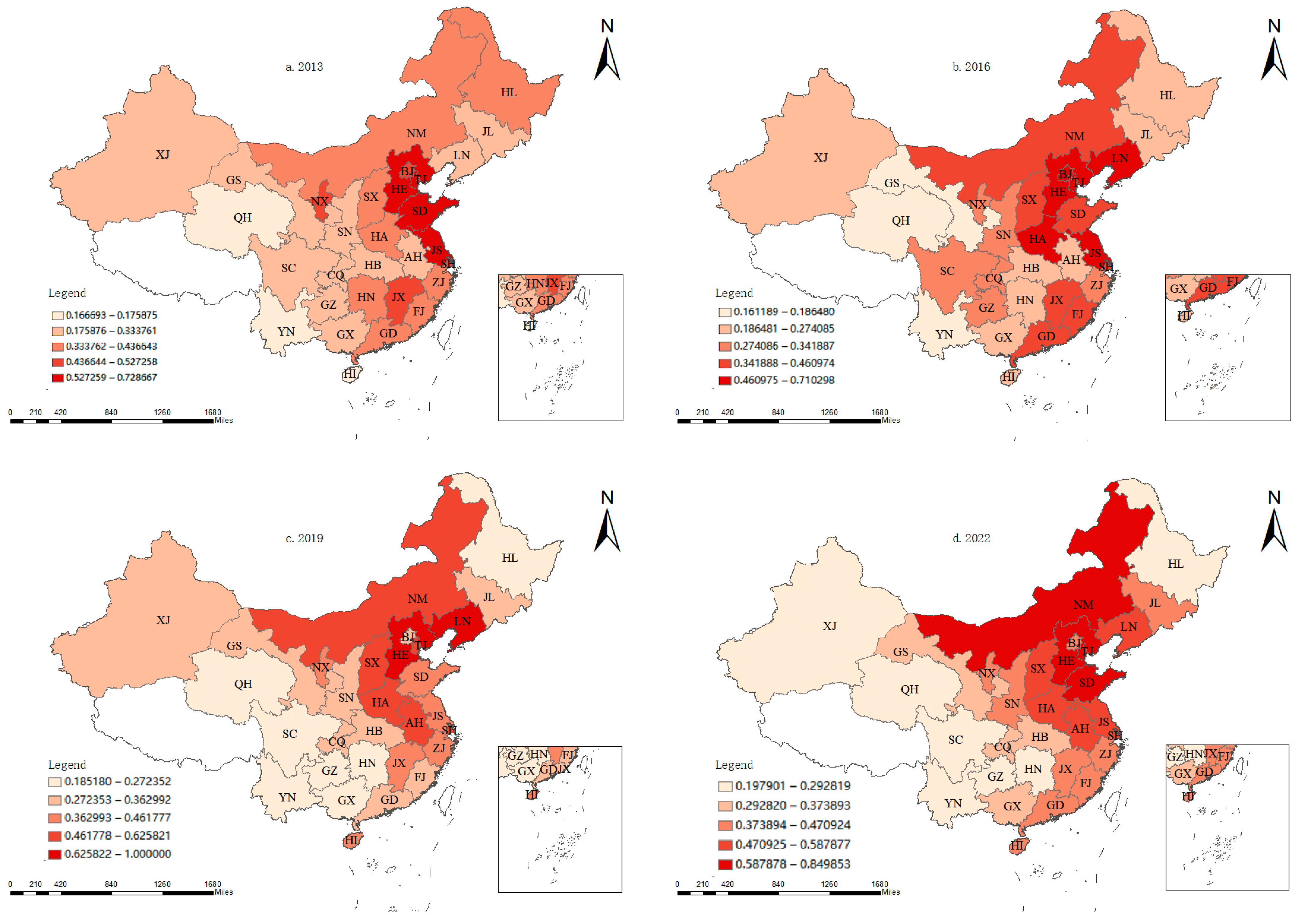
The upcoming section will employ tools like ArcGIS10.8 and GeoDa2013 to investigate spatial variations in MCAC across China’s logistics industry.
(1)
Distribution Characteristics of Marginal Abatement Cost for Carbon Emissions within the Logistics Industry
By utilizing ArcGIS software for mapping the marginal abatement costs, the analysis will focus on the years 2013, 2016, 2019, and 2022. In the legend, darker colors indicate higher MCAC values for the logistics industry.
As shown in Figure 5, Henan and Jiangsu had higher emission reduction costs in the early period, while Liaoning and Inner Mongolia had higher costs in the later period, with these cities exhibiting fluctuating cost characteristics. Qinghai and Yunnan have been among the regions with lower emission reduction costs.
(2)
Global Spatial Autocorrelation Analysis of MCAC in the Logistics Industry
Building on the prior analysis, notable spatial variations in MCAC within China’s logistics industry are evident. To investigate these spatial characteristics in greater depth, an analysis of spatial autocorrelation was performed to assess both the global and local relationships of MCAC. The global Moran’s I index for MCAC was computed, as illustrated in Table 8.
(3)
Local Spatial Autocorrelation Analysis of MCAC in the Logistics Industry
Representative years of 2013, 2016, 2019, and 2022 will be selected, and Moran scatter plots for the MCAC of the logistics industry in various provinces and cities for these 4 years will be plotted. The circles in the plots represent individual cities, with the horizontal axis indicating the MCAC within the logistics sector across various provinces and cities and the vertical axis representing the spatially lagged MCAC of the logistics industry after processing with a spatial weight matrix, as mentioned earlier.
As shown in Figure 6, from the Moran scatter plots of the aforementioned four years, it is evident that the proportion of cities in H-H and L-L consistently remains stable at around 70% of the total cities in China. This strongly indicates significant spatial clustering of MCAC in China’s logistics industry. Regions with high MCAC tend to be adjacent to other regions with high MCAC, while regions with low MCAC are adjacent to those with low MCAC. This spatial correlation reflects the non-random distribution of MCAC in the logistics industry across geographical space.
While the Moran scatter plot effectively highlights the clustering patterns between adjacent regions, it does not offer a clear visual representation of the specific characteristics of each province or city. Therefore, the LISA cluster map will be utilized to visually display the significance of each province or city. Representative years of 2013, 2016, 2019, and 2022 were selected to create corresponding LISA cluster maps.
As shown in Figure 7, from the LISA cluster maps for the representative years mentioned above, it can be observed that in 2013, 16 provinces and cities, including BJ, AH, and GX, exhibited significant spatial clustering effects. Among these, nine provinces—BJ, HE, HA, and JS, among others—exhibited H-H (high-high) clustering, while AH, HB, LN, and NM showed L-H (low-high) clustering and GX, GZ, and SC displayed L-L (low-low) clustering. The remaining provinces and cities did not show significant clustering effects.
In 2016, 11 provinces and cities, including BJ, HE, and HA, demonstrated significant spatial clustering effects. Compared to 2013, by 2016, LN and NM transitioned to H-H clustering, while HB shifted from L-H clustering to no significant clustering, and GZ moved from L-L to no significant clustering. In 2019, 14 provinces and cities, including BJ, JL, and GX, showed significant spatial clustering effects. HE, JS, LN, and other provinces exhibited H-H clustering, BJ showed L-H clustering, and GX, GZ, HI, and SC displayed L-L clustering. In 2022, 16 provinces showed significant spatial clustering effects, with 11 of them—including BJ, HE, and LN—demonstrating H-H clustering.
The spatial clustering of certain provinces and cities in China exhibits fluctuations over time. These variations are largely influenced by the ongoing transformation and modernization of China’s logistics industry, driven by efforts to lower carbon emissions and promote sustainability. The LISA cluster maps provide data for only four years. For a more comprehensive understanding of the MCAC clustering patterns across provinces and cities, the data from 2013 to 2022 are consolidated in Table 9.
The spatial clustering characteristics of MCAC in China’s logistics sector during 2013–2022 reveal distinct geographical patterns, as evidenced by Table 9. The LISA analysis demonstrates a pronounced polarization trend, with a significant majority of provincial-level regions clustering in either the H-H or L-L categories. This persistent spatial autocorrelation indicates that regions with similar MCAC levels tend to form geographically contiguous clusters, suggesting strong neighborhood effects in carbon emission patterns across provincial boundaries.
These findings carry significant implications for low-carbon logistics development, particularly in three strategic areas: (1) Formulating cross-jurisdictional carbon governance mechanisms for H-H clusters, (2) Implementing technology transfer programs between high-emission and low-emission clusters, and (3) Designing spatial econometric models to account for regional spillover effects in national carbon accounting systems. The spatial clustering patterns revealed through this analysis provide empirical support for optimizing regional collaborative governance structures and advancing targeted decarbonization pathways in China’s logistics industry.

4.3. Analysis of Influencing Factors on MCAC in the Logistics Industry

During the spatiotemporal analysis, it was found that MCAC in the logistics industry exhibits spatial dependence and heterogeneity. Therefore, a spatial econometric model will be employed to investigate the influencing factors.

4.3.1. Descriptive Statistics

In this research, the MCAC of the logistics sector from 2013 to 2022 serves as the dependent variable, while the explanatory variables include the level of economic development, investment in education, degree of innovation development, foreign capital inflow, environmental pollution, and infrastructure development. The basic statistics of the variables are presented in Table 10.

4.3.2. Correlation Tests

To examine the factors affecting the logistics industry, the LM test was initially applied to verify spatial dependencies. The results exceeded the 1% significance level for Moran’s I, LM-lag, robust LM-lag, LM-error, and robust LM-error, suggesting the need for a panel model that accounts for spatial effects. The Hausman test was performed to assess whether a fixed effects model or a random effects model would be more appropriate for the analysis. The results are presented in Table 11.
For further rigor, an LR test was performed, as shown in Table 12, to compare the performance of three models—the SDM, SAR, and SEM—based on fixed effects. The findings indicate that the Prob > chi2 values in both comparisons are below 0.1, suggesting that the fixed effects of the Spatial Durbin Model outperform those of the SAR and SEM models.
The Wald test, as detailed in Table 13, confirmed that the SDM does not simplify into either the SEM or SAR models. Consequently, the SDM was selected to analyze the determinants affecting the marginal abatement cost of carbon emissions in the logistics industry.

4.3.3. Empirical Analysis of Influencing Factors

Based on the test results presented above, it is evident that the fixed-effects Spatial Durbin Model is the most appropriate model for analyzing the factors influencing the marginal abatement cost. The fixed effects include time-fixed, individual-fixed, and two-way fixed effects. Table 14 displays the estimation outcomes for three types of fixed effects, along with the results from the OLS model. By evaluating the goodness-of-fit (R-sq) across various models, it is concluded that the results derived from the model with time-fixed effects are most appropriate for further analysis.
Based on the results shown in Table 14, the level of economic development is statistically significant in all four models, underscoring its crucial role in influencing MCAC within the logistics industry. The negative coefficient for the level of innovation development in all models suggests that improvements in innovation can lead to reductions in MCAC. According to the time-fixed effects, the analysis of influencing factors reveals that innovation development and infrastructure construction levels are significant; advancements in these areas contribute to a reduction in MCAC. Conversely, higher levels of economic development, foreign investment, and environmental pollution are associated with higher MCAC in the logistics industry.
Analyzing the spatial lag terms of the influencing variables, the coefficient for economic development in neighboring regions, the spatial lag terms of the influencing variables, and the coefficient for infrastructure construction in neighboring regions are statistically significant at the 1% level. The coefficient for economic development in neighboring regions is 0.4606. This indicates that an increase in economic development in adjacent regions raises the MCAC in the local logistics industry. Economic development exhibits notable spillover effects that stimulate growth in neighboring regions and increase emission reduction costs. Analyzing the spatial lag terms of the influencing variables, it is observed that the coefficient for economic development in adjacent regions is 0.4606. The coefficient for infrastructure construction in neighboring regions is −0.2424, indicating a strong negative spillover effect on the MCAC of local logistics industries. This influence is stronger than that of foreign investment, as demonstrated by the larger absolute value of the coefficient. However, the spatial lag terms for educational investment levels and environmental pollution factors failed the significance test, suggesting that these factors exert a lesser impact on surrounding regions.

5. Discussion

Considering China’s geographic divisions, significant variations are observed in the MCAC of the logistics sector across the four main regions. The ranking follows the order: Eastern China > Central China > Northeastern China > Western China. This observation is consistent with studies by Duan et al. and Wu et al. [10,56], which also identified significant regional disparities, particularly the higher MCAC in Eastern China compared to the Western regions. The relatively lower MCAC in the Western region can be attributed to its abundant renewable energy resources, including solar and wind power, which support low-carbon logistics operations and contribute to reducing emission-related costs. The Northeastern region, once a key industrial hub in China, has seen a decline in carbon emissions from logistics in recent years due to industrial restructuring and economic transformation. Conversely, the Central region is undergoing rapid economic growth, driving the expansion of the logistics industry and leading to increased emissions and higher MCAC. In contrast, the Eastern region, with its developed economy and advanced logistics infrastructure, faces higher energy consumption and emissions. However, this region began addressing carbon emissions earlier and has implemented diverse reduction measures, including new energy transportation technologies. As a result, its MCAC has remained relatively higher.
From the spatial distribution map depicting the MCAC in China’s logistics industry spanning from 2013 to 2022, it can be observed that TJ and HE have consistently ranked among the regions with higher abatement costs, a trend also observed in the studies by Wang et al. and Zheng et al. [57,58], which highlighted these regions’ relatively higher carbon emissions and marginal abatement costs. HA and JS exhibited higher abatement costs in the early stages, while LN and NM experienced higher costs in the later stages, with these regions demonstrating fluctuating MCAC trends over time. QH and YN have consistently exhibited lower marginal abatement costs, a trend consistent with the observations of [59,60], who highlighted the comparatively low carbon emissions in the logistics industry within these areas. The reasons for these differences are as follows: TJ and HE’s reliance on road transportation, which typically involves higher carbon emissions due to the use of fossil fuel-powered vehicles, contributes to their elevated marginal abatement costs. HA and JS, with their more favorable natural conditions and relatively lower share of energy-intensive and emissions-intensive industries, have comparatively lower carbon emissions in the logistics industry, thus leading to lower marginal abatement costs. Meanwhile, QH and YN may also benefit from better utilization of clean energy and the application of environmental protection technologies, contributing to reduced emissions and lower marginal abatement costs in the logistics industry.
Between 2013 and 2022, the MCAC of China’s logistics industry in the majority of provinces and cities primarily fell into the H-H and L-L clusters, a pattern consistent with the findings of Li et al. [61]. This indicates a significant positive spatial correlation in the MCAC of the logistics sector among provinces and cities in China, a pattern also emphasized in the research findings of Tian and Zhang [62]. Compared with international experience, studies on logistics clusters in the United States have shown that their spatial agglomeration is more significantly influenced by transportation accessibility [63]. The “logistics sprawl” phenomenon observed in cities like Chicago and Phoenix reveals the moderating effect of land costs on spatial layout [64]. These mechanisms manifest in China as a composite effect of government-led industrial park planning and market forces. Research on the location choices of logistics enterprises in the Netherlands indicates that mature logistics clusters have a significantly higher attraction for existing enterprises than for new entrants, which explains the internal logic behind the high stability of H-H type clusters in China’s Yangtze River delta region. In summary, China’s logistics industry exhibits a significant spatial polarization pattern in terms of MCAC with its highly stable cluster distribution closely related to a unique policy-driven mechanism. This provides empirical reference for differentiated paths in international carbon emission governance.
After analyzing the prevailing state of MCAC within the logistics industry, this paper delves deeper into the factors that influence it. Economic development, levels of foreign investment, and environmental pollution are key driving factors for the increase in MCAC within the logistics industry, consistent with the findings of Caetano et al. and Wang et al. [65,66]. Conversely, advancements in innovation and improvements in infrastructure help lower marginal abatement costs, aligning with the conclusions drawn by Wang and Chen [67]. Analyzing the spatial lag term of MCAC reveals that higher levels of foreign investment and infrastructure development in adjacent regions generally lead to a reduction in the MCAC of the logistics sector within local provinces and cities. In contrast, a rise in the economic development level of surrounding regions contributes to a higher marginal abatement cost in the local logistics sector. Governments can reduce carbon abatement costs in the logistics industry by attracting foreign investment and strengthening infrastructure construction. Additionally, it is crucial to consider the environmental pressures and technological challenges associated with economic development and take appropriate measures to address them.

6. Recommendations

Regional Differentiation Strategies: High MCAC Regions (e.g., Eastern China): Prioritize R&D investment in energy-saving technologies and foster cross-regional logistics collaboration for resource sharing. Low MCAC Regions (e.g., Central/Western China): Optimize existing emission reduction practices to prevent cost escalation while maintaining sustainable models.
Spatial Agglomeration-Based Policies: Provide targeted subsidies and technical support to high MCAC provinces to accelerate adoption of advanced emission-reduction technologies. Encourage low MCAC regions to refine current measures and stabilize cost-effectiveness. Promote inter-provincial logistics partnerships for joint R&D and scaled emission-reduction projects, leveraging shared resources.
Systemic Optimization Measures: Adjust economic structures toward low-carbon logistics models. Guide foreign capital toward green technology innovation. Strengthen environmental regulations to incentivize industry-wide decarbonization.

7. Conclusions

In the context of carbon emission reduction, this study calculates the MCAC of China’s logistics industry from 2013 to 2022 and examines the key factors influencing it. The findings align with China’s national conditions and development context. The main conclusions are as follows: the MCAC demonstrates a rising trend over time, showing an overall increase. From a spatial perspective, regional disparities are evident, with the Eastern region displaying the highest levels, followed by the Central, Northeastern, and Western regions in descending order. Local autocorrelation analysis reveals a positive spatial relationship in MCAC between neighboring provinces and cities. This research establishes a thorough framework for analyzing carbon reduction efforts within China’s logistics sector and delivers important recommendations for formulating low-carbon transition strategies and carbon tax market policies.

Author Contributions

Y.W.: Supervision, Conceptualization, Writing—review and editing, Methodology, Formal analysis. B.D.: Writing—original draft, Writing—review & editing, Methodology, Data curation, Formal analysis, Validation, Visualization. C.X.: Supervision, Writing—review and editing. S.W.: Data collection, Formal analysis. J.Y.: Data collection, Formal analysis. Y.Z.: Data collection, Formal analysis. All authors have read and agreed to the published version of the manuscript.

Funding

This research was funded by The National Social Science Post-Funded Project [24FJYB039], Fundamental Research Funds for Henan Provincial Higher Education Institutions [SKTD2023-02] and Major Project of Basic Research on Philosophy and Social Sciences in Henan Provincial Higher Education Institutions [2023-JCZD-15].

Institutional Review Board Statement

Not applicable.

Informed Consent Statement

Not applicable.

Data Availability Statement

All data are fully available without restriction. The datasets are taken from several public repository, https://www.stats.gov.cn/sj/ndsj/, https://cnki.nbsti.net/CSYDMirror/Trade/yearbook/single/N2022060061?z=Z024. The data presented in this study are available on request from the corresponding author.

Conflicts of Interest

The authors declare that they have no known competing financial interest or personal relationships that could have appeared to influence the work reported in this paper.

References

  1. Yang, J.; Tang, L.; Mi, Z.; Liu, S.; Li, L.; Zheng, J. Carbon emissions performance in logistics at the city level. J. Clean. Prod. 2019, 231, 1258–1266. [Google Scholar]
  2. Wang, X.; Dong, F. The dynamic relationships among growth in the logistics industry, energy consumption, and carbon emission: Recent evidence from China. J. Pet. Explor. Prod. Technol. 2023, 13, 487–502. [Google Scholar]
  3. Zhang, S.; Wang, J.; Zheng, W. Decomposition Analysis of Energy-Related CO2 Emissions and Decoupling Status in China’s Logistics Industry. Sustainability 2018, 10, 1340. [Google Scholar] [CrossRef]
  4. Wang, F.; Wang, R.; Nan, X. Marginal abatement costs of industrial CO2 emissions and their influence factors in China. Sustain. Prod. Consum. 2022, 30, 930–945. [Google Scholar]
  5. Cheng, J.; Xu, L.; Wang, H.; Geng, Z.; Wang, Y. How does the marginal abatement cost of CO2 emissions evolve in Chinese cities? An analysis from the perspective of urban agglomerations. Sustain. Prod. Consum. 2022, 32, 147–159. [Google Scholar]
  6. Wu, J.; Ma, C.; Tang, K. The static and dynamic heterogeneity and determinants of marginal abatement cost of CO2 emissions in Chinese cities. Energy 2019, 178, 685–694. [Google Scholar]
  7. Liu, J.; Feng, C. Marginal abatement costs of carbon dioxide emissions and its influencing factors: A global perspective. J. Clean. Prod. 2018, 170, 1433–1450. [Google Scholar]
  8. Li, S.; Liu, J.; Wu, J.; Hu, X. Spatial spillover effect of carbon emission trading policy on carbon emission reduction: Empirical data from transport industry in China. J. Clean. Prod. 2022, 371, 133529. [Google Scholar]
  9. Wang, Z.; He, W. CO2 emissions efficiency and marginal abatement costs of the regional transportation sectors in China. Transp. Res. Part D Transp. Environ. 2017, 50, 83–97. [Google Scholar] [CrossRef]
  10. Wu, L.; Chen, Y.; Feylizadeh, M.R. Study on the estimation, decomposition and application of China’s provincial carbon marginal abatement costs. J. Clean. Prod. 2019, 207, 1007–1022. [Google Scholar]
  11. Cristea, A.; Hummels, D.; Puzzello, L.; Avetisyan, M. Trade and the greenhouse gas emissions from international freight transport. J. Environ. Econ. Manag. 2013, 65, 153–171. [Google Scholar]
  12. Zhou, P.; Ang, B.W.; Wang, H. Energy and CO2 emission performance in electricity generation: A non-radial directional distance function approach. Eur. J. Oper. Res. 2012, 221, 625–635. [Google Scholar]
  13. Choi, Y.; Wang, H.; Yang, F.; Lee, H. Sustainable Governance of the Korean Freight Transportation Industry from an Environmental Perspective. Sustainability 2021, 13, 6429. [Google Scholar] [CrossRef]
  14. Tang, Z.; Liu, W.; Gong, P. The measurement of the spatial effects of Chinese regional carbon emissions caused by exports. J. Geogr. Sci. 2015, 25, 1328–1342. [Google Scholar]
  15. Du, Q.; Deng, Y.; Zhou, J.; Wu, J.; Pang, Q. Spatial spillover effect of carbon emission efficiency in the construction industry of China. Environ. Sci. Pollut. Res. Int. 2022, 29, 2466–2479. [Google Scholar]
  16. Wahab, S.; Imran, M.; Safi, A.; Wahab, Z.; Kirikkaleli, D. Role of financial stability, technological innovation, and renewable energy in achieving sustainable development goals in BRICS countries. Environ. Sci. Pollut. Res. Int. 2022, 29, 48827–48838. [Google Scholar] [PubMed]
  17. Chen, W.; Yang, R. Evolving Temporal–Spatial Trends, Spatial Association, and Influencing Factors of Carbon Emissions in Mainland China: Empirical Analysis Based on Provincial Panel Data from 2006 to 2015. Sustainability 2018, 10, 2809. [Google Scholar] [CrossRef]
  18. Jiang, Y.; Luo, T.; Wu, Z.; Xue, X. The driving factors in the corporate proactivity of carbon emissions abatement: Empirical evidence from China. J. Clean. Prod. 2021, 288, 125549. [Google Scholar]
  19. Guo, J.; Feng, P.; Xue, H.; Xue, S.; Fan, L. A framework of ecological security patterns in arid and semi-arid regions considering differences socioeconomic scenarios in ecological risk: Case of Loess Plateau, China. J. Environ. Manag. 2024, 373, 123923. [Google Scholar]
  20. Kang, X.; Chen, L.; Wang, Y.; Liu, W. Analysis on the spatial correlation network and driving factors of carbon emissions in China’s logistics industry. J. Environ. Manag. 2024, 366, 121916. [Google Scholar]
  21. Peng, C. Calculation of a building’s life cycle carbon emissions based on Ecotect and building information modeling. J. Clean. Prod. 2016, 112, 453–465. [Google Scholar]
  22. Shao, L.; Guan, D.; Zhang, N.; Shan, Y.; Chen, G.Q. Carbon emissions from fossil fuel consumption of Beijing in 2012. Environ. Res. Lett. 2016, 11, 114028. [Google Scholar]
  23. Wang, Z.; Geng, L. Carbon emissions calculation from municipal solid waste and the influencing factors analysis in China. J. Clean. Prod. 2015, 104, 177–184. [Google Scholar] [CrossRef]
  24. Chen, Z.; Wu, J. Evolution of Logistics Industry Carbon Emissions in Heilongjiang Province, China. Sustainability 2022, 14, 9758. [Google Scholar] [CrossRef]
  25. Cui, T.; Pan, K. An analysis and prediction of carbon emissions in the sphere of consumer lifestyles in Beijing. Environ. Sci. Pollut. Res. Int. 2024, 31, 9596–9613. [Google Scholar]
  26. Li, K.; Luo, Z.; Hong, L.; Wen, J.; Fang, L. The role of China’s carbon emission trading system in economic decarbonization: Evidence from Chinese prefecture-level cities. Heliyon 2024, 10, e23799. [Google Scholar]
  27. Liu, Z.; Xu, Z.; Zhu, X.; Yin, L.; Yin, Z.; Li, X.; Zheng, W. Calculation of carbon emissions in wastewater treatment and its neutralization measures: A review. Sci. Total Environ. 2024, 912, 169356. [Google Scholar]
  28. Xu, A.; Zhu, Y.; Wang, Z.; Zhao, Y. Carbon emission calculation of prefabricated concrete composite slabs during the production and construction stages. J. Build. Eng. 2023, 80, 107936. [Google Scholar]
  29. Zhang, N.; Zhang, G.; Li, Y. Does major agriculture production zone have higher carbon efficiency and abatement cost under climate change mitigation? Ecol. Indic. 2019, 105, 376–385. [Google Scholar]
  30. Choi, Y.; Zhang, N.; Zhou, P. Efficiency and abatement costs of energy-related CO2 emissions in China: A slacks-based efficiency measure. Appl. Energy 2012, 98, 198–208. [Google Scholar]
  31. Wang, S.; Chu, C.; Chen, G.; Peng, Z.; Li, F. Efficiency and reduction cost of carbon emissions in China: A non-radial directional distance function method. J. Clean. Prod. 2016, 113, 624–634. [Google Scholar] [CrossRef]
  32. Chen, L.; Jia, G. Environmental efficiency analysis of China’s regional industry: A data envelopment analysis (DEA) based approach. J. Clean. Prod. 2017, 142, 846–853. [Google Scholar] [CrossRef]
  33. Han, Y.; Long, C.; Geng, Z.; Zhang, K. Carbon emission analysis and evaluation of industrial departments in China: An improved environmental DEA cross model based on information entropy. J. Environ. Manag. 2018, 205, 298–307. [Google Scholar] [CrossRef]
  34. Vaninsky, A. Energy-environmental efficiency and optimal restructuring of the global economy. Energy 2018, 153, 338–348. [Google Scholar] [CrossRef]
  35. Zhang, J.; Zeng, W.; Shi, H. Regional environmental efficiency in China: Analysis based on a regional slack-based measure with environmental undesirable outputs. Ecol. Indic. 2016, 71, 218–228. [Google Scholar] [CrossRef]
  36. Chen, J.; Zhu, Y.; Yang, C.; Wang, H.; Wang, K. Evaluation and prediction of carbon emission from logistics at city scale for low-carbon development strategy. PLoS ONE 2024, 19, e0298206. [Google Scholar] [CrossRef] [PubMed]
  37. Zhang, C.; Zhang, W.; Luo, W.; Gao, X.; Zhang, B. Analysis of Influencing Factors of Carbon Emissions in China’s Logistics Industry: A GDIM-Based Indicator Decomposition. Energies 2021, 14, 5742. [Google Scholar] [CrossRef]
  38. Dai, X.; Kuosmanen, T. Best-practice benchmarking using clustering methods: Application to energy regulation. Omega 2014, 42, 179–188. [Google Scholar] [CrossRef]
  39. Chen, Y. An analytical process of spatial autocorrelation functions based on Moran’s index. PLoS ONE 2021, 16, e0249589. [Google Scholar] [CrossRef]
  40. Luo, Q.; Hu, K.; Liu, W.; Wu, H. Scientometric Analysis for Spatial Autocorrelation-Related Research from 1991 to 2021. ISPRS Int. J. Geo-Inf. 2022, 11, 309. [Google Scholar] [CrossRef]
  41. Degefu, M.A.; Argaw, M.; Feyisa, G.L.; Degefa, S. Dynamics of urban landscape nexus spatial dependence of ecosystem services in rapid agglomerate cities of Ethiopia. Sci. Total Environ. 2021, 798, 149192. [Google Scholar] [PubMed]
  42. Huo, X.N.; Zhang, W.W.; Sun, D.F.; Li, H.; Zhou, L.-D.; Li, B.-G. Spatial pattern analysis of heavy metals in Beijing agricultural soils based on spatial autocorrelation statistics. Int. J. Environ. Res. Public Health 2011, 8, 2074–2089. [Google Scholar] [CrossRef]
  43. Wang, D.; Wang, X.; Liu, L.; Wang, D.; Zeng, Z. Urban Signatures in the Spatial Clustering of Precipitation Extremes over Mainland China. J. Hydrometeorol. 2021, 22, 639–656. [Google Scholar]
  44. Huo, X.; Li, H.; Sun, D.; Zhou, L.-D.; Li, B.-G. Combining geostatistics with Moran’s I analysis for mapping soil heavy metals in Beijing, China. Int. J. Environ. Res. Public Health 2012, 9, 995–1017. [Google Scholar] [CrossRef]
  45. Yin, L.; Wang, L.; Huang, W.; Liu, S.; Yang, B.; Zheng, W. Spatiotemporal Analysis of Haze in Beijing Based on the Multi-Convolution Model. Atmosphere 2021, 12, 1408. [Google Scholar] [CrossRef]
  46. Jin, G.; Li, Z.; Deng, X.; Yang, J.; Chen, D.; Li, W. An analysis of spatiotemporal patterns in Chinese agricultural productivity between 2004 and 2014. Ecol. Indic. 2019, 105, 591–600. [Google Scholar]
  47. Zhang, M.; Wang, J.; Li, S. Tempo-spatial changes and main anthropogenic influence factors of vegetation fractional coverage in a large-scale opencast coal mine area from 1992 to 2015. J. Clean. Prod. 2019, 232, 940–952. [Google Scholar]
  48. Chen, S. Local regularization assisted orthogonal least squares regression. Neurocomputing 2006, 69, 559–585. [Google Scholar] [CrossRef]
  49. Yang, M.; Liu, H. Fuzzy least-squares algorithms for interactive fuzzy linear regression models. Fuzzy Sets Syst. 2003, 135, 305–316. [Google Scholar]
  50. Ji, D.J.; Zhou, P.; Wu, F. Do marginal abatement costs matter for improving air quality? Evidence from China’s major cities. J. Environ. Manag. 2021, 286, 112123. [Google Scholar]
  51. Su, Y.; Jiang, Q.; Khattak, S.I.; Ahmad, M.; Li, H. Do higher education research and development expenditures affect environmental sustainability? New evidence from Chinese provinces. Environ. Sci. Pollut. Res. Int. 2021, 28, 66656–66676. [Google Scholar] [PubMed]
  52. Liu, B.; Ding, C.J.; Ahmed, A.D.; Huang, Y.; Su, Y. Carbon emission allowances and green development efficiency. J. Clean. Prod. 2024, 463, 142246. [Google Scholar]
  53. Xin-Gang, Z.; Jin, Z. Impacts of two-way foreign direct investment on carbon emissions: From the perspective of environmental regulation. Environ. Sci. Pollut. Res. Int. 2022, 29, 52705–52723. [Google Scholar]
  54. Chen, Y.; Yao, Z.; Zhong, K. Do environmental regulations of carbon emissions and air pollution foster green technology innovation: Evidence from China’s prefecture-level cities. J. Clean. Prod. 2022, 350, 131537. [Google Scholar]
  55. Xie, R.; Fang, J.; Liu, C. The effects of transportation infrastructure on urban carbon emissions. Appl. Energy 2017, 196, 199–207. [Google Scholar]
  56. Duan, Z.; Wei, T.; Xie, P.; Lu, Y. Co-benefits and influencing factors exploration of air pollution and carbon reduction in China: Based on marginal abatement costs. Environ. Res. 2024, 252, 118742. [Google Scholar] [PubMed]
  57. Wang, P.P.; Li, Y.P.; Huang, G.H.; Wang, S.; Suo, C.; Ma, Y. A multi-scenario factorial analysis and multi-regional input-output model for analyzing CO2 emission reduction path in Jing-Jin-Ji region. J. Clean. Prod. 2021, 300, 126782. [Google Scholar]
  58. Zheng, X.; Wang, R.; He, Q. A city-scale decomposition and decoupling analysis of carbon dioxide emissions: A case study of China. J. Clean. Prod. 2019, 238, 117824. [Google Scholar]
  59. Dong, F.; Long, R.; Yu, B.; Wang, Y.; Li, J.; Wang, Y.; Dai, Y.; Yang, Q.; Chen, H. How can China allocate CO2 reduction targets at the provincial level considering both equity and efficiency? Evidence from its Copenhagen Accord pledge. Resour. Conserv. Recycl. 2018, 130, 31–43. [Google Scholar] [CrossRef]
  60. Ye, F.; You, R.; Lu, H.; Han, S.; Yang, L.-H. The Classification Impact of Different Types of Environmental Regulation on Chinese Provincial Carbon Emission Efficiency. Sustainability 2023, 15, 12092. [Google Scholar] [CrossRef]
  61. Li, Z.; Zhang, C.; Zhou, Y. Spatio-temporal evolution characteristics and influencing factors of carbon emission reduction potential in China. Environ. Sci. Pollut. Res. 2021, 28, 59925–59944. [Google Scholar]
  62. Tian, X.; Zhang, M. Research on Spatial Correlations and Influencing Factors of Logistics Industry Development Level. Sustainability 2019, 11, 1356. [Google Scholar] [CrossRef]
  63. Kumar, I.; Zhalnin, A.; Kim, A. Transportation and logistics cluster competitive advantages in the U.S. regions: A cross-sectional and spatio-temporal analysis. Res. Transp. Econ. 2016, 17, 16–22. [Google Scholar]
  64. Dubiea, M.; Kuob, K.C.; Giron-Valderramac, G.; Goodchild, A. An evaluation of logistics sprawl in Chicago and Phoenix. J. Transp. Geogr. 2020, 88, 102298. [Google Scholar]
  65. Caetano, R.V.; Marques, A.C.; Afonso, T.L.; Vieira, I. A sectoral analysis of the role of Foreign Direct Investment in pollution and energy transition in OECD countries. J. Environ. Manag. 2022, 302, 114018. [Google Scholar]
  66. Wang, Y.; Zhang, X.; Zhu, L.; Wang, X.; Zhou, L.; Yu, X. Synergetic effect evaluation of pollution and carbon emissions in an industrial park: An environmental impact perspective. J. Clean. Prod. 2024, 467, 142891. [Google Scholar]
  67. Wang, Y.; Chen, X. Impact Mechanism of Renewable Energy Technology Innovation on Carbon Productivity Based on Spatial Durbin Model. Sustainability 2024, 16, 2100. [Google Scholar] [CrossRef]
Figure 1. Research framework.
Sustainability 17 02839 g001
Figure 2. Carbon emissions of China’s logistics industry from 2013 to 2022 and linear fit.
Sustainability 17 02839 g002
Figure 3. MCAC in the logistics industry of China from 2013 to 2022.
Sustainability 17 02839 g003
Figure 4. MCAC in the logistics industry of four major regions in China from 2013 to 2022.
Sustainability 17 02839 g004
Figure 5. Distribution characteristics of MCAC in the logistics industry in (a) (2013), (b) (2016), (c) (2019), and (d) (2022).
Sustainability 17 02839 g005
Figure 6. Moran’s scatter plot of MCAC in the logistics industry for the years 2013, 2016, 2019, and 2022.
Sustainability 17 02839 g006
Figure 7. LISA cluster map of MCAC in the logistics industry for (a) (2013), (b) (2016), (c) (2019), and (d) (2022).
Sustainability 17 02839 g007
Table 1. Carbon emission coefficients for eight types of energy.
EnergyCarbon Emission CoefficientUnit
Raw Coal0.7559tons of carbon per ton of standard coal
Gasoline0.5538tons of carbon per ton of standard coal
Kerosene0.5714tons of carbon per ton of standard coal
Diesel0.5921tons of carbon per ton of standard coal
Fuel Oil0.6185tons of carbon per ton of standard coal
Liquefied Petroleum Gas (LPG)0.5042tons of carbon per ton of standard coal
Natural Gas0.4483tons of carbon per ton of standard coal
Electricity2.2132tons of carbon per ton of standard coal
Table 2. Standard coal conversion coefficients for eight types of energy.
EnergyStandard Coal Conversion CoefficientUnit
Raw Coal0.7143kg of standard coal per kg
Gasoline1.4714kg of standard coal per kg
Kerosene1.4714kg of standard coal per kg
Diesel1.4571kg of standard coal per kg
Fuel Oil1.4286kg of standard coal per kg
Liquefied Petroleum Gas (LPG)1.7143kg of standard coal per kg
Natural Gas1.33kg of standard coal per kg
Electricity0.1229kg of standard coal per kg
Table 3. Spatial association patterns in Moran’s scatterplot.
QuadrantSpatial Association PatternSpecific Meaning
First QuadrantHigh-High Clustering (H-H)Spatial association where a region with a high observed value is surrounded by other regions with similarly high values.
Second QuadrantLow-High Clustering (L-H)Spatial association where a region with a low observed value is surrounded by regions with high values.
Third QuadrantLow-Low Clustering (L-L)Spatial association where a region with a low observed value is surrounded by other regions with similarly low values.
Fourth QuadrantHigh-Low Clustering (H-L)Spatial association where a region with a high observed value is surrounded by regions with low values.
Table 4. Indicator system for factors influencing the marginal abatement cost in the logistics industry.
Influencing FactorsSymbol IdentificationData SourcesUnits
Economic Development Level [50] (a1)PGDPRegional GDP/Total Population at the End of the YearYuan
Education Investment Level [51] (a2)EIRand D ExpenditureTen thousand yuan
Innovation Development Level [52] (a3)IDNumber of Valid Invention PatentsPieces
Foreign Investment Level [53] (a4)FITotal InvestmentHundred million USD
Environmental Pollution [54] (a5)EPTotal Emission of Waste PollutantsTen thousand tons
Infrastructure Development [55] (a6)INFTotal Length of Postal RoutesKilometers
Table 5. Regional division.
RegionSpecific ProvincesAbbreviation
Northeastern RegionLiaoning, Jilin, HeilongjiangLN, JL, HL
Eastern RegionBeijing, Tianjin, Hebei, Shanghai, Jiangsu, Zhejiang, Fujian, Shandong, Guangdong, HainanBJ, TJ, HE, SH, JS, ZJ, FJ, SD, GD, HI
Central RegionShanxi, Anhui, Jiangxi, Henan, Hubei, HunanSX, AH, JX, HA, HB, HN
Western RegionInner Mongolia, Guangxi, Chongqing, Sichuan, Guizhou, Yunnan, Shaanxi, Gansu, Qinghai, Ningxia, XinjiangNM, GX, CQ, SC, GZ, YN, SN, GS, QH, NX, XJ
Table 6. Total carbon emissions of China’s logistics industry from 2013 to 2022 (in million tons).
2013201420152016201720182019202020212022
China16,673.5917,210.6718,087.9018,496.9019,317.6919,915.2319,410.3918,040.4019,317.7922,454.66
AH485.65532.92539.03546.95584.62601.03577.84578.99584.64515.54
BJ568.66598.09618.05648.69687.37729.54746.11487.16529.17383.95
FJ490.01531.99560.74597.70631.04671.55724.45659.63699.88665.18
GS285.97288.22267.99260.07264.15244.19244.04237.88226.52243.75
GD1533.621605.381673.351819.221904.911945.271985.531752.401678.801329.93
GX385.49485.46500.87516.51565.16548.90533.06447.64473.00517.85
GZ354.14373.15405.32446.97387.73412.50438.39448.56504.28503.12
HI161.45155.66160.95154.15163.78158.98162.18164.23175.31157.43
HE508.22465.23456.25538.15441.91504.37489.02351.76407.87451.37
HA662.97659.84709.77702.46735.31845.36837.44860.67931.75997.18
HL592.39634.35655.77663.37603.93519.41502.26426.06470.93473.91
HB729.95782.66798.01978.35990.691015.571126.44950.831117.71975.38
HN613.51670.01755.47790.24836.92895.89929.29908.43940.43926.56
JL329.22363.62381.97366.98354.44275.09274.73264.59284.32173.19
JS946.221023.871055.191084.981137.201201.081245.241276.991240.621183.30
JX351.68360.68394.39401.08417.80473.97512.97507.10513.07495.96
LN907.99981.081019.241046.571050.701034.80980.33916.19974.31887.96
NM660.59658.09674.26436.68416.83399.81411.71382.88378.25396.52
NX83.8887.6288.5991.7796.2079.3283.7879.8385.4681.33
QH66.8474.0776.2788.0098.78109.80111.5593.73103.60116.61
SD1004.541033.761050.571092.731217.471190.411210.61938.74988.961023.73
SX471.81465.27487.56500.78520.93487.24474.22375.03350.31357.27
SN405.67425.58416.60365.25366.33403.18394.37332.74337.94354.42
SH1124.661119.701173.341306.021428.551397.921452.231209.271268.211051.72
SC373.24527.09511.40743.87774.52785.90822.25774.63809.75844.46
TJ223.26236.15237.86240.47239.91241.18239.94217.49236.04222.83
XJ386.40400.73475.17496.40536.57541.40533.57431.56455.26453.13
YN527.18596.71577.87605.26617.99695.16757.11722.08745.65695.45
ZJ758.91773.45821.77825.20857.69837.76784.15818.41853.64828.08
CQ414.07385.14463.18499.95527.26466.86478.61447.59447.46372.99
Table 7. Marginal abatement costs of carbon emissions in the logistics industry for 30 provinces and cities in China from 2013 to 2022.
Province2013201420152016201720182019202020212022
AH0.32240.28930.27090.25870.26010.53640.53890.51910.53650.5554
BJ0.48230.45280.49420.50240.41090.31530.36300.36960.39960.4213
FJ0.43010.41530.42080.43110.45670.31250.31250.34620.38630.4493
GS0.28000.17550.18330.16120.18560.28660.28600.25510.29090.3211
GD0.40430.40250.38820.39190.39140.36810.35050.37030.44110.4380
GX0.32470.27550.26400.25260.25790.24090.25810.30960.33870.3234
GZ0.33380.33870.34630.33690.42090.24220.24690.24660.24730.2541
HI0.17310.21300.20900.22830.26430.28390.39340.34520.42530.4367
HE0.72870.76400.75280.71031.00000.78810.96300.61001.00000.8499
HA0.43660.52750.48170.51440.49560.53800.56950.54090.55290.5691
HL0.36460.31660.24190.24450.27770.21620.22180.23090.23660.2154
HB0.29740.29160.27560.21180.22570.30500.30240.28560.29750.3618
HN0.38020.35600.29330.27410.27260.25810.25540.26200.26790.2793
JL0.31880.29020.26110.25710.28400.34310.33670.40410.41370.4352
JS0.59880.53350.51570.51780.50470.45230.46180.47770.54080.5133
JX0.51180.42450.39250.39780.46290.45280.42180.41410.44130.4709
LN0.32560.30840.37880.54420.62270.69561.00000.80690.71460.5039
NM0.36950.36190.29750.45160.46970.60530.60340.63171.00000.6549
NX0.52730.43670.39220.34190.31590.37000.43500.46760.48800.4523
QH0.16670.16140.17250.16460.16010.17110.18520.19090.20720.1979
SD0.57520.47150.44980.46100.42320.44290.45800.57720.64250.6884
SX0.39900.37410.39610.40740.79080.66340.56030.61460.78230.5712
SN0.33020.31810.28860.31790.31300.34950.35830.43460.49240.4647
SH0.48750.57180.43700.41010.42770.48250.52440.61800.67620.5879
SC0.26180.26510.30360.29910.31420.27200.27240.28980.29260.2798
TJ0.60890.53220.53320.53470.66040.65070.62580.58990.59020.6804
XJ0.28210.25320.20770.22830.18990.23130.31460.23340.23570.2879
YN0.17590.15120.17170.18650.21910.22840.22180.22170.25520.2928
ZJ0.36010.38540.33650.34140.34460.33730.38160.36670.40230.4355
CQ0.27630.32620.29360.30080.30080.29380.31130.32460.37060.3739
0.38450.36610.34830.35600.39080.39110.41780.41180.46550.4455
Table 8. Moran’s I Index of MCAC in China’s logistics industry from 2013 to 2022.
YearMoran’s IZp-Value
20130.22873.50760.003
20140.28143.98870.001
20150.23673.45270.003
20160.32024.4890.001
20170.20953.22470.006
20180.34294.94330.001
20190.26484.26140.003
20200.36474.89910.001
20210.37315.28910.001
20220.41815.65170.001
Table 9. Spatial agglomeration types of marginal cost of abating carbon emissions in China’s logistics industry from 2013 to 2022.
Agglomeration Classification20132014201520162017
H-HBJ, HE, JS, HA, SX, SD, SH, TJ, XJBJ, HE, HA, JS, SD, SX, SH, TJ, XJBJ, HE, HA, LN, JS, SD, SX, SH, TJ, XJBJ, HE, HA, LN, JS, NM, SD, SX, SH, TJ, XJBJ, HE, LN, JS, NM, SD, SH, TJ, XJ
H-L GZ
L-HAH, HE, LN, NMAH, HE, LN, NMAH, HE, NMAHAH
L-LGX, GZ, SCQH, SCSCGX, SCGS, SC
Agglomeration Classification20182019202020212022
H-HHE, JS, LN, NM, SD, SX, SH, TJ, XJHE, JS, LN, NM, SD, SH, TJ, XJHE, JS, LN, NM, SD, SH, TJ, XJHE, LN, NM, SD, SX, TJ, XJAH, HE, HA, JS, LN, NM, SD, SX, SH, TJ, XJ
H-L
L-HBJBJBJBJBJ
L-LGX, GZ, SC, YNGX, GZ, HI, SC, YNGD, GX, SC, YN, GZGD, GX, SC, YN, GZGX, GZ, SC, YN
Table 10. Descriptive statistics results.
IndicatorsAverageStandard DeviationMinimumMaximum
Marginal emission reduction cost (y)0.3980.1630.1511
Economic development level (a1)63,838.8929,241.8923,151190,000
Education investment level (a2)4,530,0006,110,00065,0293,417,485
Innovation development level (a3)37,560.0877,935.5205573,000
Foreign investment level (a4)3240.036230.5843056,704
Environmental pollution (a5)116.64390.2534.6450.01
Infrastructure construction (a6)296,000425,00012,2083,420,000
Table 11. LM, Hausman test.
TestMoran’s ILM-LagRobust
LM-Lag
LM-ErrorRobust
LM-Error
Hausman
Statistic3.03128.95428.6457.2936.98428.72
p-value0.0020.0000.0000.0070.0080.0072
Table 12. LR test.
Table 12. LR test.
LR Chi2Prob > Chi2
SAR77.490.0000
SEM89.420.0000
Table 13. Wald test.
Chi2Prob > Chi2
13.070.0227
12.540.0510
Table 14. Spatial Durbin Model analysis of MCAC in the logistics industry.
Time-FixedIndividual-FixedDual Fixed EffectsOLS Regression
a10.0605 *0.3306 *−0.1827 ***0.1192 ***
(1.7634)(1.9361)(−2.6850)(3.4839)
a20.0055−0.1253−0.02150.0476 **
(0.2201)(−1.2785)(−0.5329)(2.0156)
a3−0.0400 *−0.0305−0.0206−0.0542 ***
(−1.7494)(−0.6170)(−0.5929)(−2.6938)
a40.0701 ***0.0565 *0.00600.0553 ***
(6.4187)(1.6927)(0.5570)(5.3821)
a50.0753 ***−0.1170 ***0.02400.0735 ***
(4.5123)(−3.2749)(0.8496)(3.8199)
a6−0.0692 ***0.0128−0.0146−0.0823 ***
(−5.6821)(0.3760)(−1.2866)(−7.1806)
_cons −0.8338 ***
(−2.5985)
wx
w × a10.4606 ***0.18260.0385
(4.7245)(1.0277)(0.2248)
w × a2−0.1213−0.1571−0.0985
(−1.3566)(−1.5660)(−0.9363)
w × a30.2408 ***−0.0453−0.0709
(3.0408)(−1.3263)(−0.7853)
w × a4−0.0886 **0.0644 **0.0141
(−2.3889)(2.0530)(0.3422)
w × a50.0050−0.0577 **−0.2957 ***
(0.0979)(−2.3465)(−3.4270)
w × a6−0.2424 ***0.0010−0.0065
(−5.7749)(0.0263)(−0.1705)
sigma2_e0.0124 ***0.0055 ***0.0047 ***
(12.2451)(12.2471)(12.1492)
R-sq0.42830.02620.07810.3940
Log-likelihood232.3453355.1706376.6624
Note: *** p < 0.01, ** p < 0.5, * p < 0.1.
Disclaimer/Publisher’s Note: The statements, opinions and data contained in all publications are solely those of the individual author(s) and contributor(s) and not of MDPI and/or the editor(s). MDPI and/or the editor(s) disclaim responsibility for any injury to people or property resulting from any ideas, methods, instructions or products referred to in the content.

