Article

Nested Optimization Algorithms for Accurately Sizing a Clean Energy Smart Grid System, Considering Uncertainties and Demand Response

by
Ali M. Eltamaly
1,* and
Zeyad A. Almutairi
1,2
1
Sustainable Energy Technologies Center, King Saud University, Riyadh 11421, Saudi Arabia
2
Mechanical Engineering Department, King Saud University, Riyadh 11421, Saudi Arabia
*
Author to whom correspondence should be addressed.
Sustainability 2025, 17(6), 2744; https://doi.org/10.3390/su17062744
Submission received: 4 February 2025 / Revised: 3 March 2025 / Accepted: 12 March 2025 / Published: 19 March 2025
(This article belongs to the Section Energy Sustainability)

Abstract

:
Driven by environmental concerns and dwindling fossil fuels, a global shift towards renewable energy for electricity generation is underway, with ambitions for complete reliance by 2050. However, the intermittent nature of renewable power creates a supply–demand mismatch. This challenge can be addressed through smart grid concepts that utilize demand-side management, energy storage systems, and weather/load forecasting. This study introduces a sizing technique for a clean energy smart grid (CESG) system that integrates these strategies. To optimize the design and sizing of the CESG, two nested approaches are proposed. The inner approach, “Optimal Operation,” is performed hourly to determine the most efficient operation for current conditions. The outer approach, “Optimal Sizing,” is conducted annually to identify the ideal size of grid components for maximum reliability and lowest cost. The detailed model incorporating component degradation predicted the operating conditions, showing that real-world conditions would make the internal loop computationally expensive. A lotus effect optimization algorithm (LEA) that demonstrated superior performance in many applications is utilized in this study to increase the convergence speed. Although there is a considerable reduction in the convergence time when using a nested LEA (NLEA), the convergence time is still long. To address this issue, this study proposes replacing the internal LEA loop with an artificial neural network, trained using data from the NLEA. This significantly reduces computation time while maintaining accuracy. Overall, the use of DR reduced the cost by about 28% compared with avoiding the use of DR. Moreover, the use of NLEA reduced the convergence time of the sizing problem by 43% compared with the best optimization algorithm used for comparison. The replacement of the inner LEA optimization loop reduced the convergence time of sizing the CESG to 1.08%, compared with the NLEA performance.

1. Introduction

Transitioning from fossil fuels to renewable energy is essential for addressing climate change and preserving the environment. Fossil fuels are accelerating climate change by releasing greenhouse gases like carbon dioxide, trapping heat, and causing rising global temperatures. The International Energy Agency (IEA) forecasts that carbon dioxide gas emissions could reach 45 billion metric tons by mid-2040, urging a swift shift towards cleaner energy sources [1]. Additionally, fossil fuels are a finite resource with a limited lifespan. Fossil fuels, while historically central to global energy, contribute to environmental harm. Conversely, renewable energy adoption, especially wind and solar systems, advances sustainability. Integrating these renewables into existing grids poses frequency stability challenges. This study examines the impact of renewable energy sources (RESs) on grid stability, supporting the global shift to cleaner energy. RESs, on the other hand, provide a sustainable, cost-effective, and environmentally friendly solution. A significant impediment to widespread renewable energy integration lies in the current infrastructure, which is primarily designed for fossil fuel-based generation. This infrastructure often lacks the flexibility to accommodate the intermittent and distributed nature of renewables. To address mitigating these limitations, we have incorporated a discussion on clean energy smart grids (CESGs). These advanced grid systems are crucial for supporting the transition to renewables by enhancing grid stability through intelligent control and enabling distributed energy storage. By facilitating the integration of diverse RESs and optimizing energy flow, CESGs play a vital role in overcoming infrastructure constraints and accelerating the adoption of clean energy technologies, thus providing a more comprehensive understanding of the solutions required for a sustainable energy future. Driven by continuous technological advancements, RESs are experiencing significant efficiency and affordability gains. This translates to increasingly competitive costs compared to fossil fuels, paving the way for a more feasible transition towards a clean energy future [2]. In essence, switching to renewable energy benefits both the environment and the economy, creating a cleaner, more sustainable future [3,4,5].

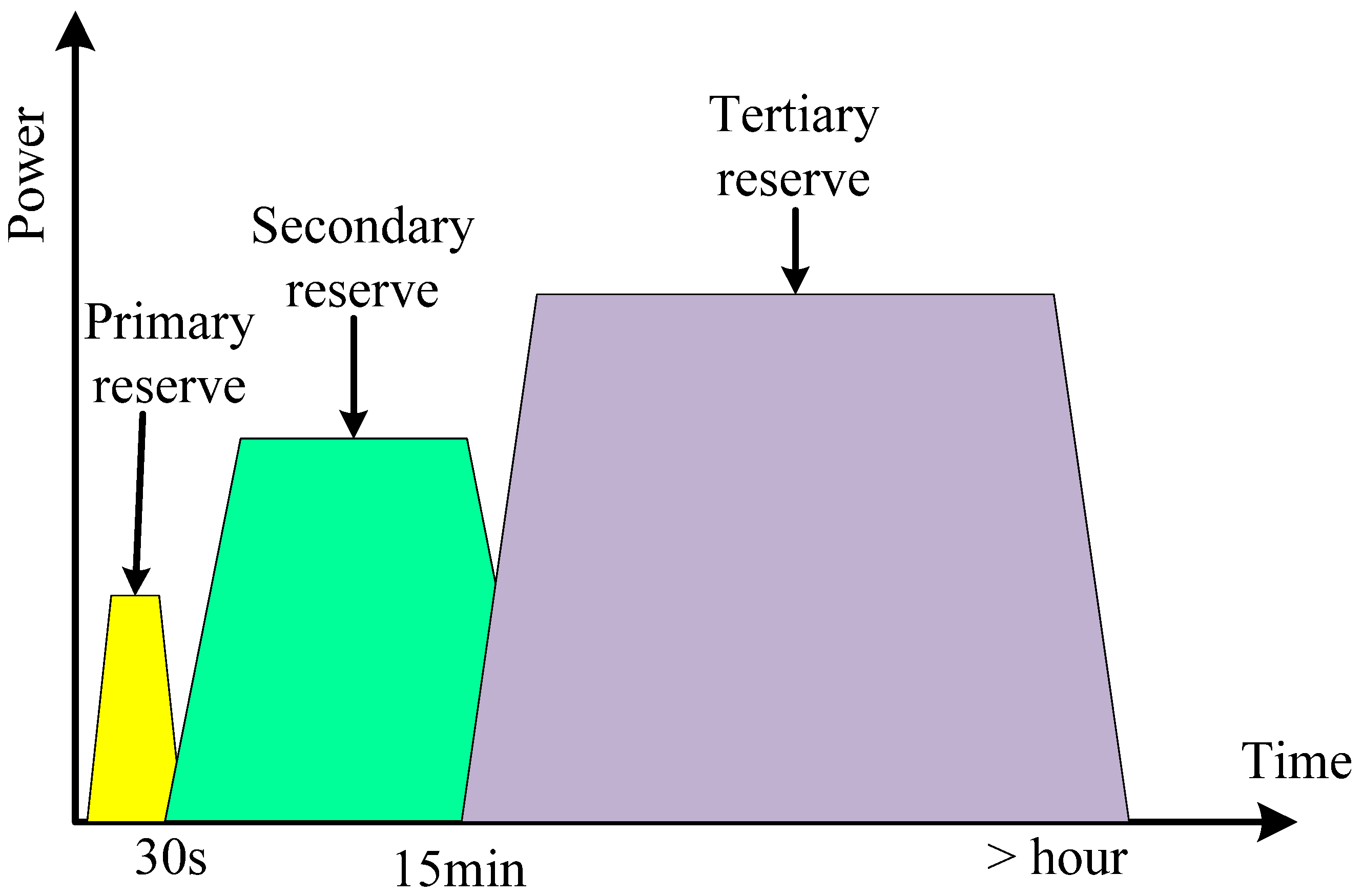
1.1. Intermittency Effect

Despite the inherent intermittency of solar and wind power systems, a multifaceted approach successfully addresses this challenge. For later use, energy storage systems (ESSs), like batteries and pumped hydro, capture excess renewable energy during peak production. Demand-side management (DSM) programs encourage energy users to consume power at a time when renewable energy is readily available. Improved weather forecasting allows for the better prediction of renewable energy generation, enabling grid operators to adjust power supplies from other sources. Moreover, connecting geographically dispersed RESs across a wider grid balances the fluctuations, as wind production in one area can be supplemented by solar power from another [6]. Furthermore, RESs, such as wind and solar systems, offer more consistent electricity compared to traditional fossil fuel-based systems. By implementing a combination of these strategies, intermittency can be significantly mitigated. Emerging at the forefront of these strategies is smart grid technologies (SGTs). These technologies represent a revolutionary leap in managing and delivering electricity from RESs. By utilizing real-time data from two-way communication and advanced sensors, smart grids optimize power flow, minimize energy loss, and enhance grid reliability and resiliency, meaning that the proactive identification of potential outages becomes a reality [7,8,9]. Empowered by real-time tariff information, consumers can make informed decisions to manage their consumption or shift their usage to cheaper off-peak hours.

1.2. Sizing of Smart Grid Components

For optimal performance, smart grids require precisely sized components. This ensures that they can effectively balance current and future energy demands and generated power. Oversized components waste money upfront and during maintenance, while undersized ones suffer from overload, outages, or even system failure. Proper sizing ensures cost-effectiveness, reliability, and efficiency. It also allows for the smooth integration of RESs by enabling sufficient storage capacity for excess energy during peak production and delivery during low-generation periods. Furthermore, by accounting for potential future growth and new technologies, correctly sized SGTs are designed to maintain their promises of efficiency, reliability, sustainability, and cost-effectiveness over an extended period.
The authors of [10] highlight the volatile nature of RESs and the resulting need for grid stability. This underscores the challenge of large-scale ESS implementation. Because RES supply is unpredictable, substantial ESS capacity is crucial for effective management, enabling energy transfer across hourly, daily, and seasonal timescales [11].
Accurate load forecasting using historical data, weather forecasts, and machine learning helps determine capacity needs for transformers and generation. RES integration is factored in through scenario analysis and probabilistic modeling to optimize energy storage for handling fluctuations and maintaining grid stability. Sophisticated market-available software simulates component behavior under various conditions to identify bottlenecks and optimize sizing for efficient operation, such as Homer [12], iHOGA [13], RAPsim [14], etc. A complete review study discussing these platforms is introduced in [15,16]. These programs do not have enough flexibility to add custom demand response (DR) or to use more accurate component degradation calculations or weather and load forecasting. These limitations have been avoided by modeling the smart grid system in MATLAB software (Version R2024a), as introduced in other studies [4,9,17]. By looking at the overall cost throughout a component’s lifetime, economic models can help in finding the most cost-effective size for parts in a project. When multiple objectives like minimizing cost, maximizing reliability, and integrating high renewable energy penetration exist, multi-objective optimization techniques with specialized algorithms search for optimal component sizes that satisfy all criteria.
Predicting future energy needs for smart grid planning is challenging, due to uncertainties in weather, demand, economics, and technology. Integrating RESs is further complicated by limited data on output patterns, hindering optimal storage sizing. Component models, while sophisticated, may not capture all real-world complexities, leading to sizing errors. Resource constraints can also limit the use of computationally intensive optimization techniques by smaller utilities. Additionally, rapid technological advancements necessitate constantly evolving sizing strategies to avoid obsolescence. Despite these challenges, the ongoing refinement of smart grid sizing techniques allows engineers to design increasingly efficient and reliable grids that are capable of high RES integration [18].
The realistic modeling of components is the key issue for successful sizing strategies of the smart grid. Many studies have not considered vital issues such as the degradation that occurs in the components, especially batteries [4,19]. Detailed degradation modeling of lithium-ion batteries (LIBs) in the sizing of the smart grid has been introduced in many studies [20,21]. Some studies did not consider degradation and soiling issues in PV arrays, for simplicity [22], while other studies assumed a certain yearly percentage reduction in capacity, for simplicity [17]. All these inaccurate models have been avoided in this study to ensure accurate sizing in the proposed smart grid system.

1.3. Energy Storage Systems

Choosing the right ESS for a smart grid requires a nuanced evaluation by considering the various technical characteristics, operational considerations, economic factors, and environmental impact. Technically, the power and energy capacity (kW and kWh) determine how much power an ESS can deliver and store, so aligning this with your smart grid’s peak power demands and desired storage duration is crucial. Additionally, you should consider round-trip efficiency, charge/discharge rate, and if the ESS’s lifetime and degradation rate are impacting replacement costs and long-term storage capacity. A critical factor in selecting an ESS for smart grids is the response time, which measures how quickly the system can begin delivering or absorbing energy. A faster response time is essential for applications that need to react swiftly to grid fluctuations. Based on the response time, ESS technologies can be categorized into three primary reserves; primary, secondary, and tertiary, as shown in Figure 1 [23].
Battery energy storage systems (BESSs) are the primary reserve because of their swift response times within milliseconds, making them ideal for primary frequency control. This fast response allows them to inject or absorb energy quickly, stabilizing grid frequency fluctuations. However, other ESS options offer valuable backup solutions for energy arbitrage. Hydrogen energy storage systems (HESSs), for example, exhibit a moderate response time in the range of seconds. These systems can be deployed as secondary reserves, acting after the BESS if the primary reserve fails to maintain the grid frequency within acceptable limits. For situations requiring an even slower but more substantial energy reserve, pumped hydroelectric energy storage (PHES) comes into play. PHES systems, with their response times measurable in minutes, function as tertiary reserves. They can be activated when both the primary and secondary reserves are insufficient to maintain grid frequency. Several studies have used one or more of these ESSs, according to the size and location of the system [1,4].
Smart grids strategically combine ESS technologies with dispatch strategies that are either predefined or optimized. Optimized dispatch balances objectives like cost and reliability. ESS selection considers safety, environmental impact, costs, and scalability. Tailoring ESS choices to specific grid needs ensures their sustainability and effectiveness. Reference [24] provides a comprehensive review of BESSs, including their history and evolving role in RES integration. This reference dives deep into techno-economic considerations for grid integration with RESs and future trends in BESS technology. Smart grid sizing studies often overlook real-world operational factors, such as component degradation, particularly battery wear [25,26,27]. Some studies have considered the yearly degradation as a percentage of the state of health (SoH) of the batteries [28], while other researchers go deeply into calculating the degradation cost of the battery based on real use [20], depending on the achievable cycle count–depth of discharge (ACC-DoD) curve. The latter study [20] used the model to represent the hourly degradation for optimal management of the smart grid but it is not used in conjunction with sizing. To the best of our knowledge, no smart grid sizing study has yet considered a realistic model for the hourly degradation of batteries, which likely affects the accuracy of the results. For this reason, this important point is avoided in the proposed study.

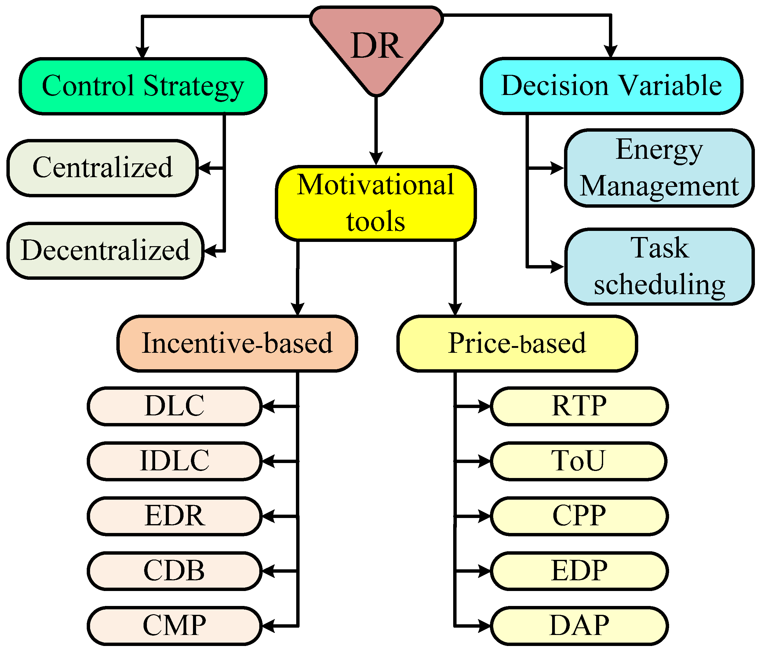
1.4. Demand Response

The DR is one of the tools of the SGT used to improve its performance in terms of cost and reliability [4,29,30,31]. The DR can be classified based on several categories such as control strategy, decision variables, and motivation tools, as shown in Figure 2. The control strategies are subdivided into centralized and decentralized DR systems. Centralized DR systems empower utilities to directly manage energy use. This can involve individually controlling devices or collaborating with customers to adjust their consumption. They monitor the grid’s energy flow, predict demand, and, during peak times, signal participants to reduce consumption [32,33,34,35]. This can be achieved through price adjustments or, with user consent, by directly controlling specific loads. While this approach offers scalability, predictability, and optimized grid management, it comes at the cost of limited consumer choice, privacy concerns, and the need for a strong communication network throughout the grid. Meanwhile, decentralized DR gives consumers the option to either participate in maintaining smart grid stability or not [21,36,37]. Price signals from smart meters nudge consumers to voluntarily reduce usage, while automated home controls can even adjust consumption based on preferences or real-time pricing. This approach offers greater consumer choice and privacy and also requires less infrastructure investment. However, it can be less predictable, due to individual behavior, and requires effort to coordinate responses from many consumers. The future likely lies in a hybrid model that combines centralized coordination with decentralized flexibility for a more sophisticated and effective way to manage energy demand [36,37].

1.4.1. Decision Variables

Smart-grid DR programs optimize energy use through two decision variables, energy management [38], and task scheduling [39], as shown in Figure 2. Energy management reduces the total consumption during peak hours through strategies like load shifting or thermostat adjustments. Task scheduling then refines this strategy, optimizing the timing of specific task use based on the DR program type, consumer preferences, and available technology. This collaborative approach between consumers and utilities unlocks the full potential of DR, creating a more efficient, sustainable energy system with lower costs for consumers and a more stable grid with reduced environmental impact [7,40].

1.4.2. Motivation Tools

Smart grids use two main strategies to manage electricity demand: price-based [4,29,30,31] and incentive-based [41,42], as shown in Figure 2. Price-based DR relies on dynamic pricing, where costs fluctuate depending on real load, generation from RESs, and the storage available in the ESS. This encourages consumers to shift their consumption to cheaper times [4,29,30,31]. Incentive-based DR rewards users directly for reducing or shifting their energy use during peak periods [41,42]. While price-based DR is simpler and offers consumer choice, it requires user understanding and may not impact large consumers. The price-based DR is subdivided into time-of-use (ToU) pricing and real-time pricing (RTP), extreme day pricing (EDP), critical peak pricing (CPP), and day-ahead pricing (DAP). RTP DR is a common strategy for optimizing smart grid operations, but many strategies did not consider it during the sizing process [4,25,29,30,31,43].
Another study suggested the RTP formula for the dynamic tariff in terms of the state-of-charge (SoC) and the BESS power [31]. This study modeled the system DR but did not consider other important issues, such as the forecasted weather and load variables [31]. A fuzzy logic controller, incorporating the previous hour’s tariff change, overcomes this limitation and improves performance [29] and the forecast factor, considering the day-ahead weather and load operation [4]. Incentive-based DR offers targeted participation and guaranteed reduction but can be more complex for grid operators [41]. The best approach depends on specific grid needs, consumer preferences, and program goals. The future likely involves combining both approaches for a more efficient and sustainable energy system. A hybrid incentive-based and price-based DR strategy is also discussed in [41]. Incentive-based DR is subdivided into direct load control (DLC), emergency DR (EDR), indirect load control (IDLC), customer demand bidding (CDB), and central main power (CMP). Detailed review studies were introduced elsewhere in the literature to compare between all of these DR strategies [40,44]. The authors of [25] categorized loads as high-priority (essential under all conditions) and low-priority (shiftable based on system operations), as a clear application of the DLC DR strategy.
A recent study [45] proposed a smarter way to manage energy use in smart grids. It combines optimal scheduling that prioritizes efficiency with a layered architecture that allows for autonomous management by diverse consumers. This could lead to automated energy use that is both cost-effective and reduces overall consumption. However, for this approach to work best, electricity tariffs need to consider factors like peak hours and consumer behavior to incentivize participation and optimize energy use across the entire grid [45]. Several review papers in the literature are used to summarize the efforts of suggesting the tariff according to the situation of the smart grid operating conditions [40,46,47].

1.5. Optimization Algorithms

While SGT offers superior reliability, efficiency, resiliency, and cost reduction, it also comes with a computational burden. Traditional optimization algorithms, requiring calculations hourly throughout the year (8760 times), can significantly slow down smart grid operations and sizing. Several studies have explored optimization algorithms for hybrid renewable energy systems (HRES) [48,49,50,51,52,53]. The authors of [50] reviewed optimization techniques when applied to HRES, while Bhandari et al. [51] provided a broader overview of HRES optimization, encompassing various sizing techniques. Notably, graphical techniques can be effective for problems with only two sizing variables, offering a clear and intuitive representation [52,53]. Kaabeche and Ibtiouen [48] employed an iterative technique within MATLAB to optimize a smart grid system in Algeria. Their focus was on achieving a zero total energy deficit by adjusting the PV panels, wind turbine numbers, and battery capacity. Smaoui et al. [49] also utilized an iterative technique in MATLAB but used different HRES configurations. They optimized a combined PV, wind turbine, and HESS with desalination for a community of 14,400 inhabitants. This research highlights the versatility of iterative techniques for optimizing various renewable energy configurations.
Smart grid component sizing utilizes a toolbox of optimization algorithms, each with its own specialty. Linear programming (LP) is a reliable technique for linear problems, offering quick initial assessments but also struggling with complexities [54]. Mixed-integer linear programming (MILP) [55] tackles whole-number variables like transformer capacity but can be computationally expensive for intricate problems. Non-linear programming (NLP) [56] handles real-world non-linearities but requires more setup and solving effort compared to LP or MILP. Heuristics and metaheuristics [29,31,57,58,59,60,61,62,63,64,65,66,67,68,69], are iterative searchers that find good solutions quickly for complex problems with non-linearity but do not guarantee absolute optimality. Finally, multi-objective optimization techniques find compromises between multiple objectives like cost and reliability using methods like Pareto optimization. Several optimization algorithms have been introduced for sizing the smart grid systems such as particle swarm optimizations (PSO) [58,59,60,61,62,63], genetic algorithms (GA) [57], cuckoo search (CS) [29,64,65], grey wolf optimization (GWO) [66,67], the bat algorithm (BA) [31], musical chairs algorithm (MCA) [69], etc. Other studies have used hybrid optimization algorithms in the sizing of smart grid systems to enhance the optimization performance [68].
A nested optimization algorithm that uses the internal one to perform the hourly optimal operation and the external one to perform the optimal sizing of smart grid components is needed because of high computational challenges that increase the convergence time and reduce the accuracy. Many benchmark optimization algorithms such as BA, PSO, CS, GWO, and GA have been studied to perform this optimization task, but they show very long convergence times. For this reason, a modern optimization algorithm shows its superiority by fast and accurate performance in optimizing several engineering problems; the lotus effect optimization algorithm (LEA) [70] is used for this task. The nested LEA is provided here to optimize the optimal operation problem in the inner loop and the optimal sizing problem in the outer optimization loop. Although the LEA substantially reduced the convergence time, there is still a need for further reduction. For this reason, this study proposes a novel approach to address this computational challenge. An artificial neural network (ANN) is used later to replace the internal LEA optimization loop, which reduces the convergence time to less than 1.08% of the nested LEA (NLEA). The proposed ANN is trained from the existing NLEA algorithm’s results. This innovative approach offers potential smart grid efficiency improvements and will be validated subsequently.

1.6. Main Innovation and Contribution

This study provides a sizing strategy for an autonomous CESG system considering the real modeling of different components, along with real dispatch strategies considering RTP DR and an accurate degradation model for LIBs and other components. Key contributions of this work include:
1-
Developing accurate CESG component models.
2-
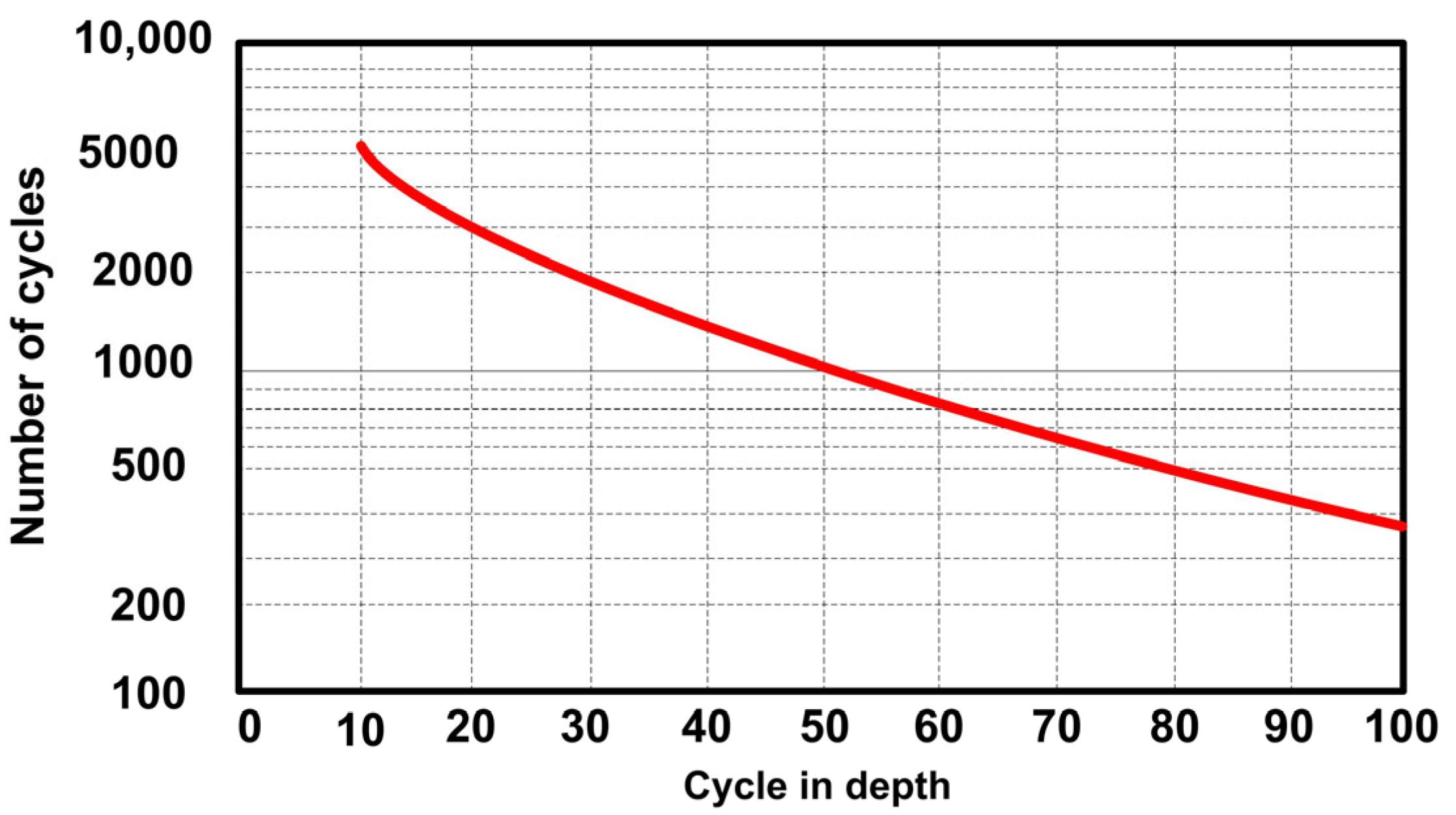
Creating a new hourly model for LIB degradation.
3-
Implementing a real DR strategy considering the current charge level (CCL) of the ESS, the day-ahead weather, and load levels.
4-
Introducing optimal dispatch strategy for the power flow between the RESs, the loads, and the ESS.
5-
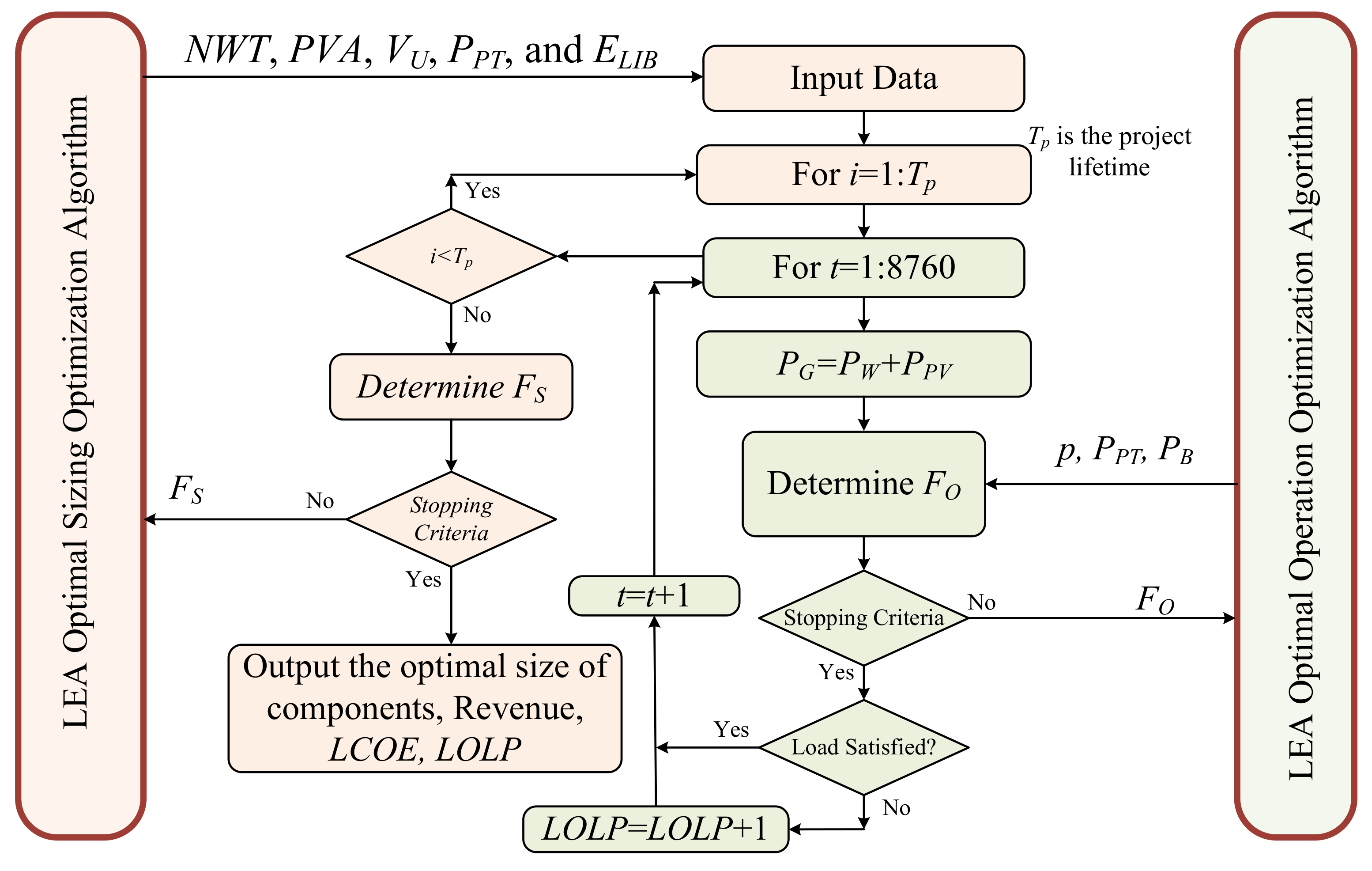
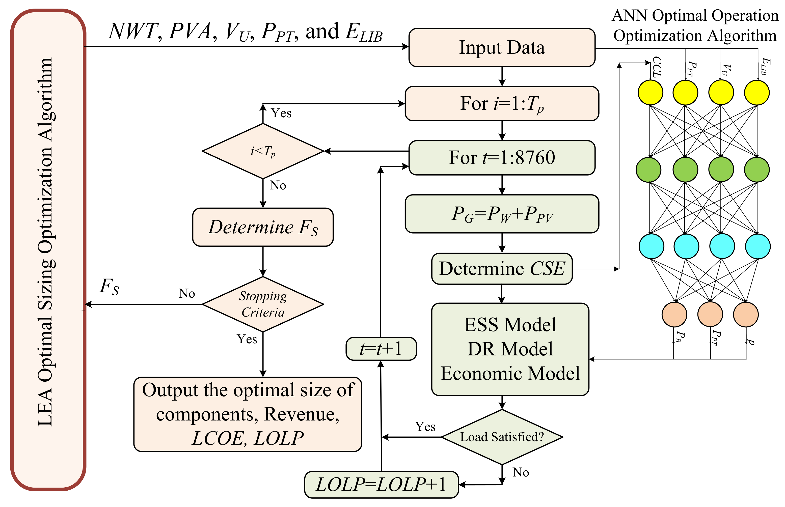
Implementing a nested LEA for optimal operation in the inner optimization loop and optimal sizing in the outer loop.
6-
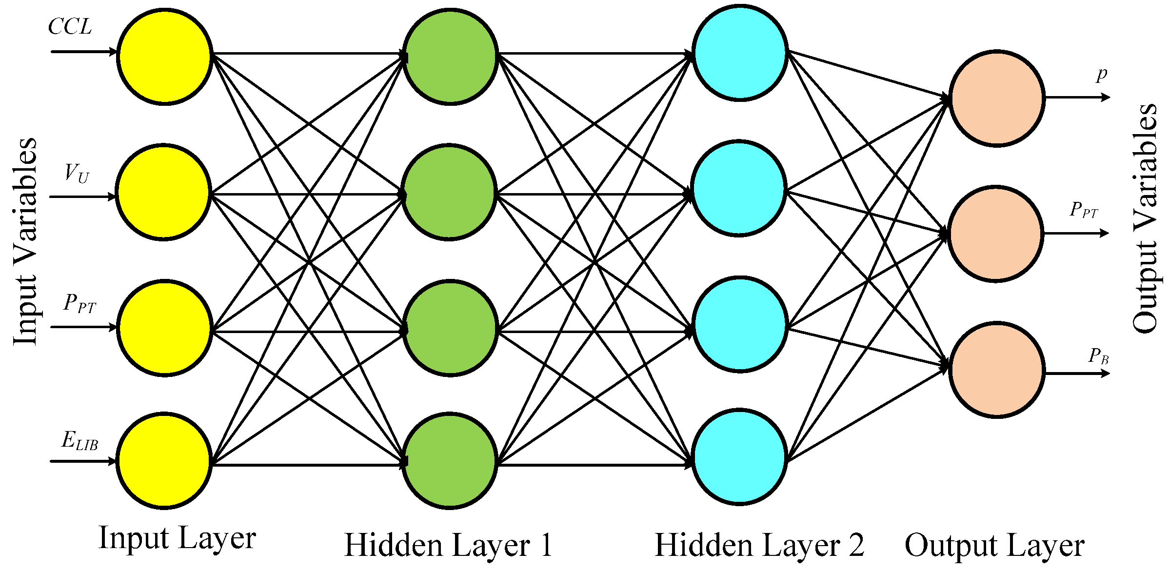
Introducing an ANN strategy for replacing the inner optimization loop to substantially reduce the convergence time of the proposed sizing strategy.

1.7. Study Outlines

This study establishes a strong foundation by first providing a comprehensive overview of smart grids and the need for CESG systems. Section 2 then delves into the typical configuration of a CESG, detailing the roles of RESs, ESSs, control systems, and DR in managing energy consumption. Section 3 introduces and discusses the performance of the NLEA for efficient problem-solving. It further details how this section explores replacing the NLEA loop with an ANN to improve the convergence time for CESG sizing optimization. Section 4 details the software used to implement various models, including those for CESG components, dispatch strategy, DR, battery degradation, economic analysis, and optimization algorithms. Key simulation results showcasing the study’s most significant findings are presented in Section 5. Finally, Section 6 concludes the research by summarizing the key points, offering recommendations, and outlining potential areas for future exploration.

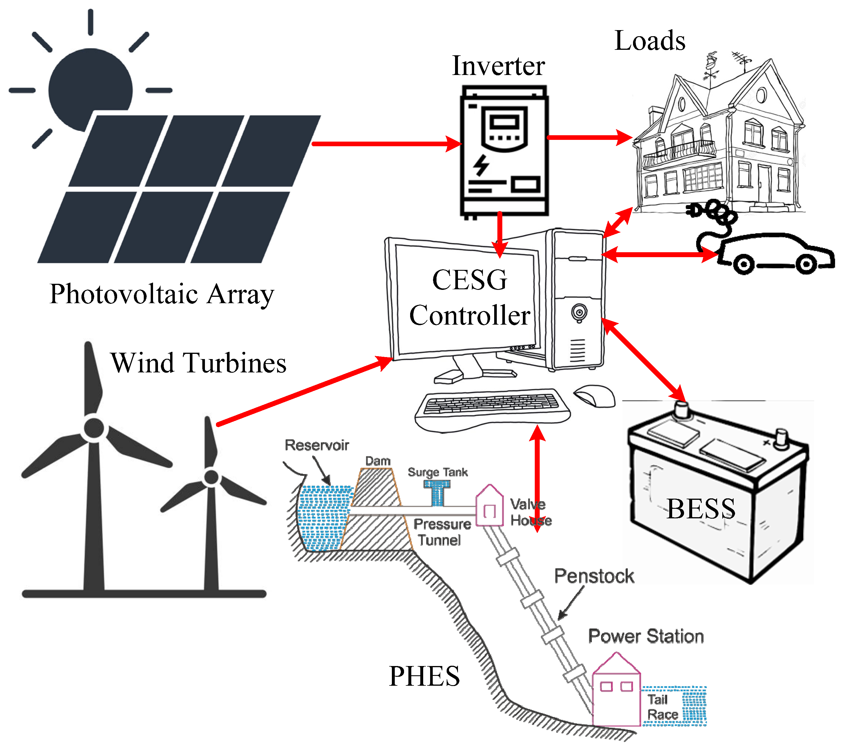
2. Smart Grid System Configuration

The smart grid configuration regularly includes RESs, ESSs, and control systems, as shown in Figure 3. CESGs, unlike conventional smart grids, eliminate traditional power plants. They mitigate renewable energy intermittency via ESSs, employing fast-response BESSs like LIBs for frequency regulation, and PHES for energy arbitrage. A price-based RTP DR controls the loads [4,25,29,30,31,43].

2.1. Modeling of CESG

Precise component sizing is vital for CESG success. Oversizing inflates costs and maintenance, while mismatch impairs system efficiency, and under-sizing is equally harmful. Accurate component models, reflecting real-world conditions, are essential for simulation-driven optimization. This section details the modeling of key CESG components.

2.1.1. Modeling of Wind Turbines

Accurate wind turbine (WT) modeling requires accurate wind speed, direction, turbulence, and shear profile data, along with detailed technical specifications from the WT manufacturer. Analytical models offer computational efficiency but may lack accuracy in complex scenarios. Conversely, computational fluid dynamics (CFD) provides detailed aerodynamic information but demands significant computing power. Comparing model predictions with real-world performance data and established models helps identify and rectify discrepancies.
The wind speeds measured at the anemometer’s height hg need to be modified to match the wind speeds at the height of the WT (hWT). Equation (1) illustrates the relationship between the anemometer wind speeds at WT height, along with the height of the anemometer [71].
u ( h W T ) = u ( h g )     h W T h g α
The following formula displays the hourly produced power from the WT at wind speed u [71]:
P w v = 0 u U C     &   u U F         P R u k U C k U R k U C k , U C u U R       P R U R u U F
where the WT cut-in speed, rated speed, and cutoff speed are denoted by UC, UR, and UF, respectively.

2.1.2. Modeling of the Photovoltaic System

Accurate modeling of a PV energy system requires high-quality data, including historical and, ideally, site-specific solar irradiance and ambient temperature information. To account for efficiency losses, comprehensive specifications should be obtained from the PV module manufacturer, as well as information on temperature coefficients, efficiency, and P-V curves along with information on other system components, including inverters, maximum power point trackers (MPPTs), and ESSs. This thorough method will help designers create a PV system model that is precise and dependable, which is essential for design optimization, energy production prediction, and guaranteeing financial viability.
Tilting the PV modules at the ideal tilt angle is advised to maximize irradiance and, in turn, the energy produced by the PV system. The site’s latitude angle is taken into consideration while selecting this ideal tilt angle [71]. Equation (3) is used to calculate the PV array’s hourly produced power:
P P V t = H t t P V A η c t
where Ht is the solar radiation on an ideally tilted surface [71], PVA is the net area of the PV array, and ηc(t) is the hourly efficiency of a photovoltaic array, which can be calculated from the following equation:
η c t = η c r 1 β t × T c t T c r
where βt is the temperature coefficient and its value, as used in this study, is 0.004 per °C [72], the solar cell efficiency is expressed as ηcr, while the temperature is expressed as Tcr. With the following equation, the instantaneous solar cell temperature Tc(t) at ambient temperature (Ta) can be calculated [72]:
T c t = T a + 3 H t t

2.1.3. Modeling of the BESS

Accurate modeling of the BESS for CESG requires comprehensive data, with BESS specifications such as cell chemistry, capacity, power rating, efficiency curves, and cycle life. Moreover, an accurate hourly degradation for the BESS is essential. By employing this comprehensive approach, designers can achieve a reliable BESS model for smart grid applications. This model will be utilized in optimizing BESS operation, maximizing grid benefits and ensuring its economic viability and long-term performance.
There are several methods utilized in the production of LIBs, and the majority of them have different cathode materials. Because of its long lifespan, high level of safety, high power density, high round-trip efficiency, wide working temperature range, and affordable price, lithium iron phosphate (LiFePO4) is the most suitable technology [73]. Within the LIBs, two distinct degradations take place: calendar-related degradation and cycling-related degradation. The operating temperature and the SoC have a direct relationship with calendar-related degradation. Cycling degradation increases with temperature and charge/discharge power but decreases with SoC. Numerous studies have presented the degradation of LIBs [74,75,76,77]. Accurate models based on the real calendar and a cycling test are also presented in the literature [21,30,78,79].
Model parameters are determined by minimizing the root mean square error (RMSE) between model-calculated and test-derived degradation data. This laboratory-based assessment of LIB degradation is crucial for project success, especially because highly accurate manufacturer data are often unavailable. The relationship between the DoD and the ACC, as seen in Figure 4, is mostly supplied by manufacturers [21]. This is the reason why this curve serves as the basis for the unique degradation model of LIBs in this study.
The mathematical model presented in Equation (6) is used to represent the relationship between the DoD of the LIB and the ACC [21]:
A C C = a   ·   D o D b
where the curve shown in Figure 4 is used to determine fitting parameters a and b.
Equation (7) indicates that the DoD is equivalent to the difference between the maximum and minimum SoC:
D o D L I B t = 1 E L I B t E L I B R = 1 S o C L I B t
where E L I B t and E L I B R are the stored energy of the LIB at time t and the rated capacity, respectively.
Equation (8) may be utilized to determine the SoH of the LIB, which is the ratio of its rated capacity ( E L I B R ) to its maximum stored energy ( E L I B max ).
S o H = E L I B max E L I B R
Equation (9) shows the LIB’s throughput energy, accounting for charging/discharging efficiency and capacity fade [21].
E T = 2   ·   η L I B 2   ·   A C C   ·   D o D   ·   E L I B R   ·   1 + θ 2
The LIB requires replacement when its capacity reaches a threshold, θ. This threshold is typically 40% for stationary BESS applications [4] and 80% for electric vehicles [21].
Using Equation (9), Equation (10) yields the degradation density function (DDF), representing LIB deterioration per kWh [21].
D D F = 1 E T = 1 η L I B 2   ·   A C C   ·   D o D   ·   E L I B R   ·   1 + θ  
As seen in Equations (11) and (12), respectively, the DDF may be expressed in terms of DoD and SoC, based on Equations (6) and (10), respectively.
D D F = 1 η L I B 2   ·   a     ·   E L I B R   ·   1 + θ   ·   D o D b 1 = 1 η L I B 2   ·   a     ·   E L I B R   ·   1 + θ   ·   1 S o C b 1
D D F = K D   ·   D o D b 1 = K W   ·   1 S o C b 1
where K D = 1 η L I B 2   ·   a     ·   E L I B R   ·   1 + θ .
Because the simulation assumes constant hourly charge/discharge power (Δt), the charge/discharge ramp is modeled hourly. Equation (13) then calculates the total hourly wear [80].
D L I B t = t 1 t 1 + Δ t E L I B R   ·   D D F t ( S o C ) d S o C ( t ) d t   d t
Equation (14) calculates the change in SoC ( d S o C ( t ) d t ) over time.
d S o C ( t ) d t = P L I B E L I B R
The following equation calculates the LIB degradation occurring within each hour (Δt, as defined in this study):
D L I B t = K D   ·   P L I B 2 b   ·   E L I B R 1 S o C int + P L I B   ·   Δ t E L I B R b 1 S o C int b
where SoCint denotes the initial SoC during each ramp.

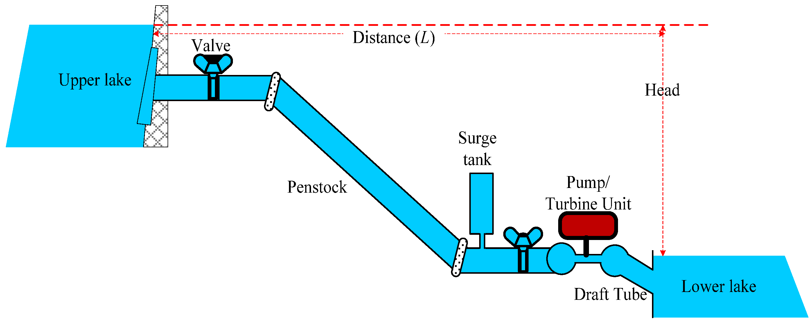
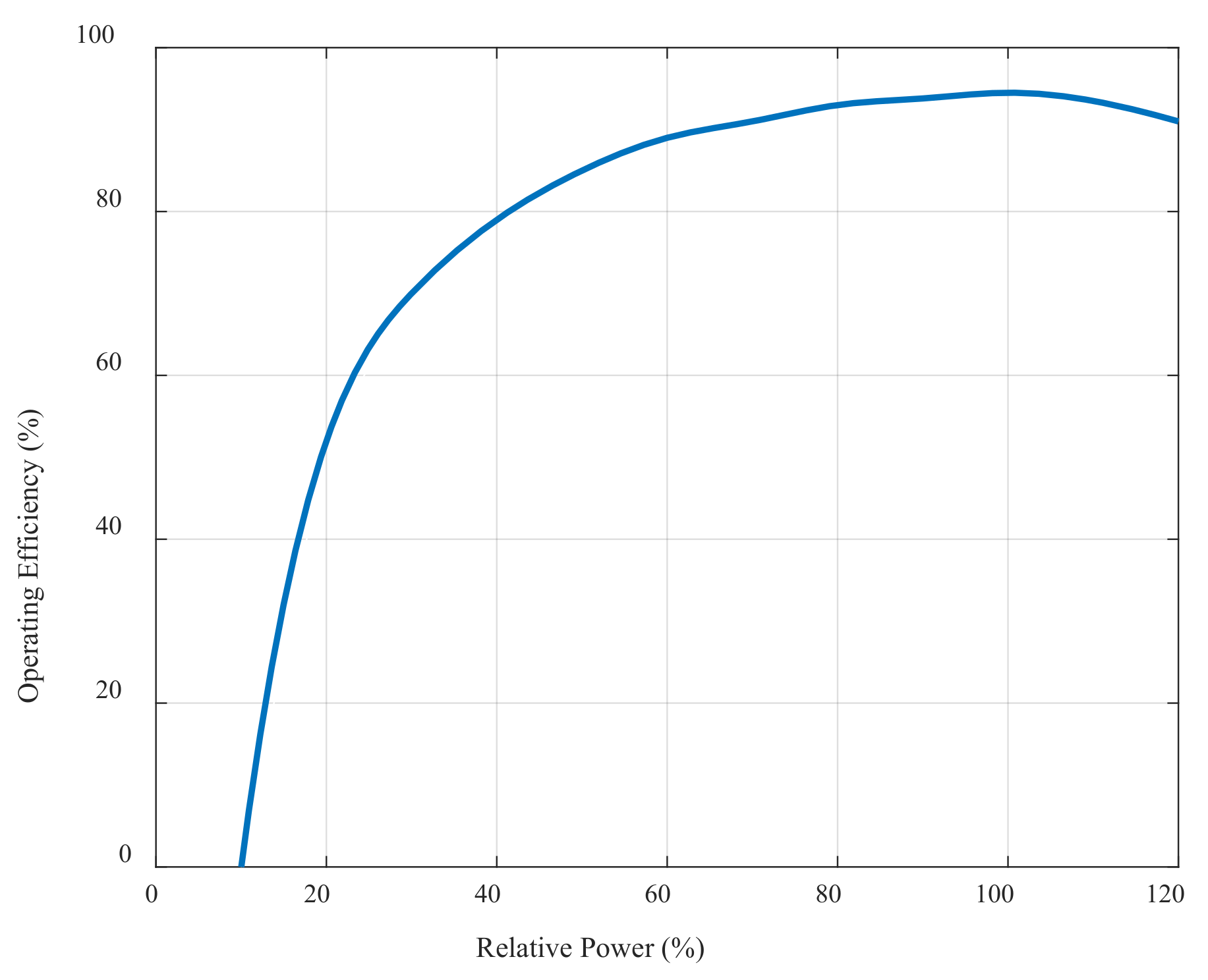
2.1.4. Modeling of PHES

Accurate modeling of PHES requires a multifaceted approach. First, comprehensive site data are gathered, including reservoir capacities, elevation differences, and waterway characteristics. Detailed technical specifications of the pump-turbine units, encompassing efficiency curves, power output, and limitations are also necessary. Next, a combination of modeling techniques is employed. Hydraulic models simulate water flow dynamics, accounting for head losses. Electrical models analyze the electrical behavior of the system, including the conversion efficiencies. Finally, system-level models integrate both aspects for comprehensive PHES operation simulation. Finally, we consider environmental impacts like water evaporation and ecological changes, and incorporate economic factors like operation and maintenance costs, energy market prices, and revenue streams to assess the project’s economic viability.
For energy arbitrage within the CESG, PHES proves to be the most suitable option. Figure 5 shows how PHES pumps water up to a higher reservoir during excess energy periods, releasing it back to the grid during low generation. Both reservoirs will be filled with a combination of desalinated water and rainwater. The PHES system can be equipped with pump-turbine units in either binary or ternary configurations. These units combine a turbine and a pump, connected to electric machines. Binary units, despite being more common due to their lower cost and compact size, are slower and less adaptable.
A key drawback of PHES is its slow response time, particularly during startup or sudden changes in power demand. While ramping up from a standstill to full capacity can take several minutes, even transitioning from half- to full capacity requires at least 15 s [81]. This sluggish response necessitates the use of batteries to manage rapid fluctuations in grid conditions. In this context, the combination of a PV energy system (solar panels) with PHES offers an attractive and cost-effective solution for energy arbitrage [81].
The efficiency and effectiveness of a PHES facility hinges on the turbine and pump combination. Reversible Kaplan, Francis, and Pelton turbines are among the types of turbines that can be used in PHES facilities. A few of the variables that affect these decisions include the flow rate, the necessary starting speed (ramp-up time), and the water pressure (head). Because they are efficient, adaptable, and suitable for most PHES operating situations, Francis and reversible Kaplan turbines are the most widely chosen options [81]. This study prioritizes Francis turbines for PHES, due to their key advantages: lower initial cost, simpler design, and sufficient efficiency, particularly when combined with a BESS. A BESS effectively mitigates the slower ramp-up rate inherent in Francis turbines, making them suitable for applications requiring a fast response to power fluctuations. Figure 6 depicts the variation in the efficiency of Francis turbines relative to their power output [81,82].
Several studies have been suggested to ascertain the ideal penstock diameter [83,84,85]. Warnick et al. [83] proposed an empirical formula (16) to determine the ideal penstock diameter, based on the rated flow (Q). They also suggested a diameter calculation (Equation (17)) based on head difference (h) and rated power ( P P H E S R ). Equation (17) has been applied in the study simulation, where the rated power of the PHES fluctuates according to the optimization recommendation, while the head is maintained as constant.
D e = 0.72   Q 0.5
D e = 0.72   P P H E S 0.43 / h 0.63
Penstock head friction loss modeling efforts are summarized in Ref. [84]. From Equation (18), one can determine the head friction loss [84]:
h f = 0.0826   f   Q 2   L D e 5
where L is the penstock length (1200 m, based on the NEOM site’s topology), and f is the friction factor (0.32–0.36) [84].
The effective head associated with pump operation is equivalent to the sum of the actual head and the head loss due to friction (Equation (19)). Conversely, the effective head during turbine operation is defined as the difference between the actual head and the head loss resulting from friction (Equation (20)).
h = h t + h f in   pump   mode
h = h t h f in   turbine   mode
Equation (21) displays the power generated by the turbine-generator unit [86]:
P T t = η T   ρ w   h   g   Q T t
where ρw is the water density (1000 kG/m3), g is the gravitational acceleration, and Q T t is the discharge flow rate (m3/s). ηT is the efficiency of the turbine-generator unit.
Equation (22) provides a method for calculating the power of a pump-motor unit [86]:
P P t = Q P t ρ w g h / η P
where QP represents the pump’s flow rate.
Equation (23) determines the gravitational potential energy (EU) of the upper reservoir [86].
E U = η T   ρ w   ( V U t V min )   g   h
In the upper reservoir, Vmin represents the minimal volume, while VU represents the current water volume. According to recommendations made in Ref. [87], the upper reservoir should be designed to maintain a minimum capacity of 5% of its rated value.
Equation (24) calculates the new upper reservoir volume. According to this equation, in the pump mode, the flowrate through the turbine (QT) is equal to zero, and in the reverse situation is as follows:
V U t + 1 = V U t Q T t + Q P t Q L o s s t ·

2.2. Optimal Dispatch Strategy

Achieving an accurate model for an optimal dispatch strategy in smart grids requires a multifaceted approach. First, comprehensive data should be gathered on the grid’s physical layout (topology), component capacities (power plants and ESS), and forecasted electricity demand and renewable energy generation. Next, power flow analysis tools should be employed to simulate electricity flow and identify potential issues. Various optimization algorithms, like LEA, will then determine the optimal dispatch strategy, considering these factors. Rigorous validation through historical data comparison and scenario testing with outages, peak demand, and renewable fluctuations is crucial. Finally, cost modeling (fuel, maintenance, market prices), reliability constraints (voltage stability, outage risk), and environmental considerations (emissions) should be incorporated for a holistic dispatch strategy. By following this comprehensive approach, designers can develop an accurate model that optimizes energy dispatch, minimizes costs, ensures grid reliability, and promotes renewable energy integration.

2.2.1. Demand Response Implementation

Smart grids rely on dynamic pricing models to balance electricity use and optimize grid stability. ToU tariffs offer predictable costs with pre-set peak and off-peak hours, but limit grid operator control. RTP informs consumers of real-time prices, allowing for more dynamic control but requiring a more complex system [30,31]. This study proposes a new one-hour-ahead, forecast-driven, dynamic RTP strategy. This approach benefits both consumers through potential cost savings and grid operators through reduced peak demand and the smoother integration of RESs, leading to a more sustainable and efficient smart grid. RTP has advantages in terms of grid stability and flexibility, but it can be difficult to deploy. It depends on a careful balancing act between fair pricing and CESG stability, as well as a complex communication infrastructure. In order to overcome these obstacles, a unique pricing method that is implemented 1 h ahead is presented, optimizing grid reliability, customer cost, and user satisfaction. This strategy makes use of a multi-objective function, which, as the next subsections demonstrate, carefully balances these conflicting aims. The load’s elasticity determines how much the load changes as a result of a tariff adjustment. Price elasticity of demand (PED), as demonstrated in Equation (25) [31,63], quantifies the change in load power resulting from a change in tariff and is used to calculate the elasticity of the load. PED value, which is given as a percentage, indicates how much demand will be adjusted in response to price changes. Because of the elastic load, the amount of load requested changes significantly in response to a slight change in price. In the meantime, changes in price have little effect on the quantity requested, due to the inelastic load. In this study, numerous PED values have been simulated and examined to determine how PED affects the CESG system’s performance.
P E D = Δ P L t / P L A Δ p t / p 0
Here, PLA is the average load power and Δ P L t is the change in load power as a result of the tariff adjustment. The hourly and base tariffs are represented by pt and p0, respectively.

2.2.2. Clean Energy Smart Grid Reliability

Clean energy smart grid reliability can be assessed using indices like LOLP and LOEE (Equations (26) and (27)) [4]. To ensure a highly reliable CESG, these metrics should be considered during the design phase.
L O L P = i = 1 8760 t o u t a g e ( i ) / 8760
toutage, which equals 0 otherwise and 1 if the HRES is unable to fully feed the electric loads with their demands, is the period during which the system is unable to entirely feed the load with each need.
L O E E = t = 1 8760 P d e ( t ) / t = 1 8760 P L ( t )
Pde(t) represents the HRES’s unmet energy demand at time t.
Equation (28) calculates the forecast factor (FF), to model the hourly difference between RES-generated energy and demand, considering both current and anticipated discrepancies
F F t = 1 N F   ·   P L A i = 1 N F P G t + i P L o t + i P L A   ·     i
The original demand power at i hours ahead is P L o t + i , and the number of anticipated hours is denoted by NF. The produced power from RESs is represented by P G t + i , and i is a variable ranging from 1 to NF hours ahead.
Equation (29) calculates the ESS’s current charge level (CCL) using the battery and PHES reservoir energy, plus the anticipated load-generation difference derived from the predicted factor (FF).
C C L t = R V U t + E B R E U R ·   S o C B t + F F
E B R is the battery’s rated capacity, E U R is the PHES reservoir’s rated capacity, S o C B t is the battery’s current SoC ( S o C B t ), and R V U t (calculated in Equation (30)) is the ratio of the current to maximum reservoir volume.
R V U t = V U t V U min / V U R V U min

2.2.3. The Revenue of the CESG

Hourly revenue is defined as the difference between total income and the total expenses incurred within a given hour. Income is derived from the product of load power and the applicable tariff. Expenses are categorized as either fixed costs, which are invariant concerning operational activity, or variable costs, which are a function of operational activity. These typically represent hourly asset costs. Conversely, variable costs, as shown in Equation (31), fluctuate based on real-time equipment usage. Examples include battery degradation and the potential replacement costs associated with ESSs, like batteries and PHES units. The constant cost component is obtained by multiplying the fixed cost by the load power PL(t), as seen in Equation (32), which reflects the levelized cost of energy (LCOE). Battery degradation and PHES maintenance costs fluctuate over time and are classified as variable expenses.
Re v t = p t · P L t C c t C v t
Re v t = p t L C c t · P L t P H E S O & M t   ·   P P H E S t D C B E S S t
The variables employed in the cost and revenue analysis are defined as follows: PHESO&M denotes the hourly operation and maintenance costs of the PHES per kilowatt; PPHES represents the power processed by the PHES; DCBESS signifies the hourly degradation cost of the battery energy storage system (BESS); PL designates the modified load power, the value of which may be derived from Equation (15) in the case of LIBs; LCc represents the hourly levelized cost attributable to constant costs; and pt denotes the hourly tariff.
Equation (33) calculates the CESG’s hourly constant cost by dividing the net present cost of assets by the total project hours.
L C c t = N P C C   ·   C R F T P   ·   8760
TP is the project duration (in years); the net present cost of assets (NPCC), which can be calculated from Equation (35), and the capital recovery factor (CRF), which can be found in Equation (34), are all given:
C R F = r 1 + r T P 1 + r T P 1
where r is the interest rate.
N P C C = I C + R C + O M C c S A L
This equation calculates a value based on the original cost (IC), replacement cost (RC), constant operating and maintenance cost (OMCc), and salvage price (SAL).
Equation (36) shows that the initial cost (IC) of the CESG system includes all costs, from components and feasibility studies to consultancy and installation.
I C   =   W T I C   +   P V I C   +   B A I C   +   P H E S I C
WTIC, PVIC, BAIC, and PHESIC represent the initial costs of wind, PV, BESS, and PHES systems, respectively
The wind turbine initial cost (WTIC) is determined by the product of the number of turbines and the unit cost per turbine. The photovoltaic (PV) system installation cost (PVIC) is calculated as the product of the required area and the cost per unit area. The battery acquisition cost (BAIC) for LIBs is given by the product of the total capacity (kWh) and the cost per unit capacity (kWh). This BAIC represents the upfront cost of the battery system. Equation (37) can be used to calculate the total power capacity costs, which include the costs of both the wind turbines and the BEES:
B A I C   = C E   ·   E B R
where E F B R is the energy capacity of the LIBs, and CE is the cost per kWh capacity of the LIBs.
Equation (38) calculates the total initial cost of the PHES by adding the pump-turbine unit cost and the upper reservoir dam cost:
P H I C I C = V U R v u C   +   P P H E S R   ·   p P H E S C
where P P H E S R is the PHES unit’s rated power, p P H E S C is the pump-turbine unit cost per kW, and v u C is the dam cost per m3 of reservoir volume.
The present replacement cost of any device d is shown in Equation (39).
R C d = i = 1 N R d I C d 1 + r T P   ·   i N R d + 1
Let ICd be the component d’s starting cost, and NRd be the replacement number of d that may be determined via Equation (40):
N R d = R o u n d u p     T P L T d 1
where LTd stands for component d’s lifespan.
The two components of OMC are known as the constant OMC and the variable OMC, which is based on actual component use. The constant component of OMC is determined by schedule maintenance. The constant OMC, which is derived from Equation (41), is dependent on the size of each component and is calculated as a percentage of the component’s starting cost.
O M C c = i = 1 T P Y e a r l y   O M C r + 1 i
After retired devices approach the end of their useful lives, the salvage price may be calculated when selling them; this information can be found in Equation (42).
S A L d = i = 1 N R d + 1 S A L   Price r + 1 T P   ·   i N R d + 1
Based on battery deterioration, which can be established using Equation (15), the variable cost of the BESS is determined.
Equation (43) calculates the PHES hourly variable operating and maintenance costs, based on the turbine-pump unit’s start-up and wear costs, V P H E S O & M t :
V P H E S O & M t = μ S + P P H E S t   ·   p P H E S
where μ is the flag for the previous operation of the PHES ( P P H E S t   > 0 ), either equal to 0 or to 1, depending on whether the PHES was operating during the preceding hour of P P H E S t   > 0 . S is the PHES startup cost, signifying the amount needed to bring the PHES from a standstill to full operation, and p P H E S is the variable OMC of the PHES per kW.

2.2.4. Satisfaction Factor

The measure of customer satisfaction is the customer satisfaction factor. This factor, which is a ratio of the original power, as indicated in Equation (44), quantifies the difference between the original load power and the changed power as a result of the RTP. Taking into account the flexibility of various loads, the adjusted power consumption will automatically reduce when electricity rates (tariffs) rise. Customer unhappiness (shown by a negative satisfaction factor) might result from this modification. Tariff reductions, on the other hand, encourage higher power use beyond the initial level and may enhance consumer satisfaction. Thus, to guarantee that customers have a favorable impression of the system, it becomes imperative to maximize the satisfaction factor.
S F t = P L t P L o t

2.2.5. Multi-Objective Functions

This study utilizes two multi-objective functions to optimize the CESG system’s performance. An hourly function determines the ideal power flow by considering factors like the CCL of the ESS and revenue, as detailed in Equations (29), (31), and (44). These factors are combined into a single objective function (Equation (45)) that prioritizes maximizing three key aspects: maximizing the CCL of the ESS in Equation (29), maximizing the system’s hourly income, calculated using Equation (44), and maximizing the satisfaction factor of the customers. This combined approach ensures that the CESG system achieves optimal techno-economic function.
F O t = m 1   ·   C C L t + m 2   ·   Rev t + m 3   ·   S F t
For every individual objective function, m1 through m3 represent the weight values that must meet the criteria indicated in Equation (46).
m 1 + m 2 + m 3 = 1
The second multi-objective function is used to optimally size the components of CESG, based on minimizing the LOLP and the LCOE, as shown in Equation (47):
F S = L C O E + m L O L P
where m is the weight value used to give the LOLP the required rate, based on the required reliability. In the case of the highest reliability required from the proposed system, the value of m should be as high as possible.

2.2.6. Energy Balance Modeling

The power grid’s stability can be affected by the variable nature of weather-dependent renewable energy sources (RESs). This mismatch between generated power and load can be addressed by ESSs. However, ESS technology can be expensive and significantly increase the overall energy cost. In pursuit of a balance between system reliability and cost-effectiveness, this study proposes a synergistic methodology integrating energy storage systems (ESSs) with demand-side management (DSM) strategies.
This integrated approach facilitates optimal power dispatch among the CESG components, resulting in a substantial reduction in the dimensions of the ESS and other constituent elements.
When there is a surplus of generated power from RES (combined wind and solar power, PG = PW + PPV) exceeding loads, the excess power (PD) is used for ESS charging. An optimization algorithm, guided by the multi-objective function in Equation (45), determines how much of this surplus goes to the ESS and how much is still available to meet the remaining loads. Conversely, when there is a power deficit (PD < 0), the shortfall is compensated for by discharging power from the ESS. Additionally, DSM strategies are employed using the RTP tariffs to adjust consumer electricity consumption patterns. The multi-objective function in Equation (45) again plays a role in optimizing this process.

3. Optimization Algorithm

In smart grids, optimization algorithms are vital for efficiently planning for and sizing various components. These algorithms deliver a range of objectives such as minimized costs by finding the ideal mix and size of equipment (considering upfront costs, operational expenses, and potential revenue streams), improved efficiency through optimized component operation that reduces energy losses, enhanced reliability by determining the optimal reserve capacity and generation mix, to handle fluctuations and ensure that peak demand can be met, and increased renewable energy integration through optimized dispatch strategies that balance supply and demand despite variable renewable sources. Due to the nested optimization algorithm loops, the convergence time is very long. For this reason, a fast and accurate LEA optimization algorithm is used in the two nested optimization loops, as discussed in the following subsections.

3.1. Lotus Effect Optimization Algorithm (LEA)

The LEA is a new nature-inspired tool for solving optimization problems [70]. It draws inspiration from two key phenomena in the pollination of lotus flowers. LEA borrows ideas from the efficient pollination process observed in lotus (Nelumbo nucifera) flowers. This process involves both biological (cross-pollination) and non-biological (self-pollination) mechanisms. The phenomenon of self-cleaning observed in lotus leaves is referred to as the lotus effect. Water droplets rolling off the leaves pick up dirt and debris, keeping the surface clean. The LEA’s flexible design allows it to adapt to various optimization problems by incorporating problem-specific details into its exploration and exploitation phases. This versatility makes the LEA a powerful tool for tackling a wide range of engineering challenges. While still under development, the LEA shows promise for efficient problem-solving by mimicking the natural world’s balance between exploration and exploitation, offering a novel and bio-inspired approach to optimization. The LEA was analyzed with a wide range of benchmark functions in Ref. [70] and was also analyzed with engineering applications in [70,88,89], showing very promising results compared to other optimization algorithms. The rationale for selecting this strategy in the present study lies in its suitability for the accurate determination of optimal system size, which is contingent upon the consideration of hourly optimal operation and DR mechanisms.

3.1.1. Exploration Phase (Pollination)

Similar to cross-pollination, this phase involves exploring the search space for promising solutions. It utilizes a dragonfly metaphor, where virtual dragonflies explore the search space, exchanging information about potential solutions that they encounter. This exploration helps identify diverse regions of the search space, potentially leading to optimal solutions. During exploration, the LEA mimics real-world dragonfly behavior by incorporating three principles: separation (avoiding collisions), alignment (matching neighbors’ velocity), and cohesion (staying close to the swarm center). Additionally, the algorithm considers “food” (attractive areas) and “enemies” (areas to avoid) as factors that guide the swarm’s movement. Mathematical formulas are then used to update individual dragonfly positions within the swarm, based on these principles [70,90].
The mathematical model representing the separation between the search agents is shown in Equation (48):
S i = j 1 M X i X j
where Xi represents the current search agent position, Xj is the jth search agent position, and M is the number of neighboring individuals.
The mathematical model representing the alignment between search agents is shown in Equation (49):
A i k = j 1 M V j k M
where Vj represents the jth search agent velocity.
Cohesion represents how close the search agent is to the swarm center and is ascertained using the following equation:
C i k = j 1 M X j k M X i k
The position of the ith search agent food source can be obtained from the following equation.
F i k = X b e s t k X i k
X b e s t k is the position of the main source of food, which can be determined from the global best position.
Distraction from enemies is mathematically modeled by:
E i k = X w o r s t k + X i k ·
X w o r s t k represents the position of the enemy, which is ascertained using the worst position.
The velocity of the search agents, which shows the trajectory direction of the search agents, can be obtained from Equation (53):
V i k + 1 = s S i k + a A i k + c C i k + f F i k + e E i k + ω   ·   V i k
where s, f, a, c, and e are the separation, food, alignment, cohesion, and enemy factors, respectively, and ω is the inertia weight value.
After calculating the velocity of each search agent, as shown in Equation (53), the new search agent position is calculated from Equation (54).
X i k + 1 = X i k + V i k + 1
Some search agents should be set to fly in random motions to improve the performance of exploration; this may be achieved by applying the Lévy flight technique. The following equation calculates the new location of flying search agents using Lévy flights:
X i k + 1 = 1 + L e v y ( x ) X i k
where L e v y ( x ) is the search agents’ trajectory, based on the random fly distance. This can be determined using the equation below [70]:
L e v y ( x ) = 0.01   ·   σ   ·   r 1 r 2 1 / β
where r1 and r2 are the random numbers between 0, 1. β is a constant number, and σ can be obtained from the following equation:
σ = Γ ( 1 + β ) · sin π · β / 2 Γ 1 + β 2 · β ·     2 β 1 2           ·

3.1.2. Extraction Phase (Self-Cleaning)

This phase is inspired by the self-cleaning lotus effect and focuses on refining and improving potential solutions. Water droplets rolling on the leaves represent the movement of information between solutions. This information exchange helps eliminate “dirt” (inferior aspects) from the potential solutions, leading to a gradual improvement in their quality. In this pollination method, a coefficient defines each flower’s growth area around the best flower found. Solutions move towards this best solution, with larger steps initially and smaller steps later.
X i k + 1 = X i k + R X i k X b e s t
Here, X b e s t is the global best solution, and R is the radius of the growth area, which can be calculated from Equation (59) [70]:
R = 2 e 4 k I T max 2
where I T max is the total number of iterations.

3.1.3. Benefits of the LEA

The LEA efficiently explores the search space for promising solutions, mimicking the way that water droplets traverse the micro/nanostructures on the leaf’s surface [70]. This exploration phase leverages operators inspired by dragonfly movement patterns to identify diverse areas within the problem landscape. Once promising regions are identified, the LEA transitions to an exploitation phase. This balanced strategy prevents getting stuck in local optima, a common pitfall for optimization algorithms. The LEA dynamically focuses on both venturing into new areas of the search space (exploration) and exploiting high-potential regions (exploitation). The pseudo-code summarizing the logic of the LEA is shown in Figure 7. The LEA is used in the optimal operation of the proposed CESG in the internal loop and will be used for sizing in the outer loop, as shown in Figure 8.

3.2. Replacing Internal LEA Using ANN

Neural networks complement optimization algorithms during smart grid component sizing by offering a data-driven approach. They can learn complex relationships from historical load data, weather patterns, and renewable energy generation, capturing non-linear factors that traditional methods might miss. This is particularly beneficial for increasingly complex smart grids with diverse resources. ANNs adapt to grid evolution by continuously learning from new data, keeping sizing recommendations relevant. They also excel at handling large datasets and complex models, making them scalable for extensive smart grid systems and potentially offering faster solutions for optimizing the size of CESG systems. However, ANNs are limited by their dependence on training data quality/quantity and the nature of their hidden layers. Additionally, training large networks requires significant computational resources. Overall, while ANNs offer a promising approach for smart grid component sizing, due to their data-driven adaptability and potential speed, their limitations necessitate careful consideration alongside traditional optimization algorithms for optimal decision-making in smart grid planning.
ANNs, as illustrated in Figure 9, are bio-inspired systems that replicate aspects of brain structure and function through the interconnection of artificial neurons arranged in layers. Each neuron processes weighted inputs via an activation function and sends the output to the next layer. By adjusting these connections’ weights, the network learns patterns and relationships in the data. During operation, an input vector is fed into the network. Hidden layers process this data using activation functions, and the output layer produces a result. The ANN is exposed to labeled data (inputs with desired outputs), calculates the error between its predictions and the desired output, and adjusts weights using backpropagation to minimize this error. This iterative process continues until the network achieves good accuracy on unseen data. The efficacy of a neural network to discern complex patterns is contingent upon several factors, including the number and configuration of hidden layers and neurons, the selection of activation functions, and the quality of the training data employed. While computationally expensive to train, ANNs are powerful tools for tasks like pattern recognition, classification, and prediction, uncovering hidden data relationships and making data-driven decisions.
The input/output data and results for a complete year and for several sizes of components are collected from an optimal dispatch strategy that uses the NLEA optimization algorithm to train the ANN. The four input variables fed into the ANN module are the current charge level (CCL) of the ESS, the rated volume of the upper tank, the rated power of the pump/turbine unit comprising the PHES, and the storage capacity of the BESS. Three output variables are obtained from the ANN; these are the optimal tariff and the contribution (kW) from the BESS and the PHES. The output from the ANN will be transmitted to the PHES and BESS models to determine their new performance, with the ANN output values as shown in Figure 10. It is clear from this study that the ANN can replace the tedious calculations of the inner LEA optimization algorithm, which significantly reduces the convergence time.

4. Software Implementation

This section is dedicated to the development of software aimed at determining the optimal sizing of the CESG system. It integrates a nested LEA framework, in which the internal optimization loop is replaced by an ANN. The implemented software translates each component’s model into MATLAB code (version 2024a) and is executed on a system equipped with an Intel i7-7500U processor (2.70 GHz, dual-core) with 32 GB of RAM, and running Windows 11. Figure 8 illustrates a flowchart outlining the main model with the nested LEA. For this implementation, input data relevant to NEOM city in Saudi Arabia, as cited in Ref. [4], are utilized. The outer LEA loop determines the appropriate size of key system elements, including the number of wind turbines, photovoltaic array size, and the capacity of the BESS and PHES, as well as the rated volume of the upper reservoir for the PHES. These computed values are then forwarded to the internal loop, which relies on wind turbine and photovoltaic array models to calculate the highest possible power extraction from renewable energy sources. This power is subsequently compared to the system’s demand, taking into account constraints such as the energy storage system’s charge control limit and a forecasting factor that influences the operational objective function (FO) detailed in Equation (45).
The internal LEA optimization loop refines crucial parameters such as pricing and the required energy contributions from BESS and PHES (p, PB, PPT). The process iterates until the CESG system achieves an optimal state wherein FO reaches its maximum possible value. At this point, the updated parameters for (p, PB, PPT) are proposed. The system then evaluates whether energy demand is fully met. If not, a loss of load is registered by increasing the LOLP counter; otherwise, the operation advances to the next hourly interval, as depicted in Figure 8. This iterative approach continues throughout the full project duration, ultimately determining the sizing objective function, as formulated in Equation (47).
Throughout the process, the algorithm consistently verifies the stopping conditions for the sizing optimization procedure. If these conditions are not satisfied, the system undergoes further optimization adjustments, refining FS until convergence is achieved. Once the stopping criteria are met, the optimization process ceases, providing the final output, which includes the optimal sizes for smart grid components, projected financial returns, LCOE, and LOLP.
The external LEA optimization loop will keep optimizing the size of components to yield the highest reliability at minimal cost by minimizing the sizing objective function (Fs) shown in Equation (47).
The proposed sizing strategy shown in Figure 8 has two nested LEA optimization algorithms. Therefore, we should perform the energy balance for a complete year for each search agent of the internal LEA optimization loop. This means that the number for executing the optimal objective function can be obtained from the following equation:
N o _ n e s t = 8760   ·   N e   ·   S S e   ·   N i   ·   S S i
where SSe and Ne are the number of search agents and the iterations of the external LEA optimization loop, respectively. SSi and Ni are the number of search agents and iterations of the inner LEA optimization loop, respectively. As an example, if the number of search agents and iterations of the internal and external LEA optimization algorithms are both 50, based on Equation (60), the program should perform the dispatch strategy and hourly cost parts for 5.475 × 10¹⁰ times. This requires several hours of processing by the supercomputer to perform the whole series of sizing steps. For this reason, in this study, the internal LEA optimization loop is replaced with the ANN module, which reduces the execution of the dispatch strategy and the hourly cost, as shown in Equation (61):
N o _ A N N = 8760   ·   N e   ·   S S e
where SSe and Ne are the number of search agents and iterations of the external LEA optimization loop, respectively.
Based on our previous example, the number of calls for the dispatch and hourly cost module is 2.19 × 10⁷, which means that the sizing steps take only 0.04% compared to the use of nested LEA algorithm, which proves the superiority of replacing the internal LEA optimization loop with the ANN.

5. Simulation Results

The simulation framework incorporates hourly wind speed, solar radiation levels, and temperature data from the NEOM site as key input variables [4]. To evaluate the effectiveness of the proposed software, multiple simulation scenarios have been executed. The first scenario examines the system’s performance in both the presence and absence of the RTP DR strategy. The second simulation assesses how the nested LEA optimization algorithm performs in comparison to other optimization techniques, focusing on accuracy and convergence speed. The third investigation highlights the advantages of substituting the inner LEA optimization process with an ANN, particularly in terms of improving convergence efficiency. A detailed examination of these three simulation cases is presented in the subsequent subsections.

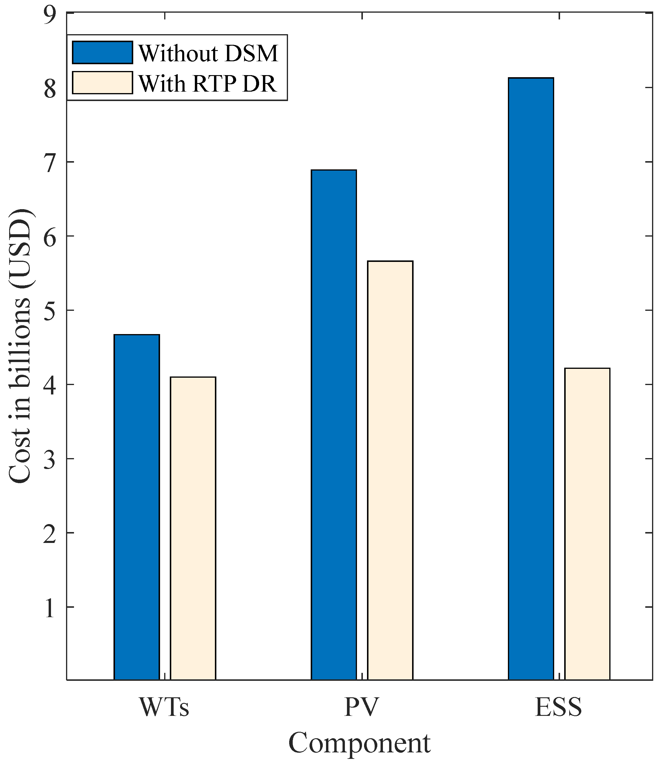
5.1. Importance of the DR Strategy

The first simulation evaluates the impact of incorporating the RTP DR strategy in comparison to a scenario where DSM is not applied for managing load demands. In this analysis, the LIB and PHES are used as energy storage systems (ESSs). The simulation model operates under the condition of PED = 0 (no DR), as illustrated in Figure 11 and Figure 12. Figure 11 shows the various parameters, including the power produced by wind and PV, the load consumption, power balance, FF, the proportion of water in the upper reservoir relative to its full capacity, the state of charge (SoC) of the LIB, and the CCL of the ESSs. Figure 12, on the other hand, illustrates the fluctuations in power balance, water levels in the reservoir, PHES power generation, and the charging/discharging cycles of the LIB, as well as the SoC and SoH of the LIB.
The primary results for the no-DR case (PED = 0) are summarized in Table 1, which shows an LCOE of USD 0.0931/kWh and a net present cost of USD 19.258, with a net present value (NPV) of 6.357. In contrast, a second case is explored where the RTP DR strategy is applied with PED = −0.5, as shown in Figure 13 and Figure 14. In Figure 13, the first trace illustrates the difference between the original and modified load demands, while the second trace represents the power balance. Additional details are provided in Figure 13, such as the forecast factor, the water volume ratio in the upper reservoir, the SoC of the LIB, the CCL, and the tariff variations. Figure 14 delves deeper into power balance variations, ESS status, and system configurations.
Table 2 presents a comparison of the key results from the two scenarios, one without DSM (PED = 0) and the other with DSM (PED = −0.5). The findings reveal that adopting the RTP DR strategy leads to a reduction in LCOE from USD 0.0931/kWh to USD 0.0625/kWh, which is a 32.87% decrease. Furthermore, the revenue generated by the CESG system with DSM (PED = −0.5) rises to USD 12.778 × 10⁹, which is more than double the USD 6.357 × 10⁹ revenue generated when DSM is not used. This highlights the substantial improvement achieved through RTP DR implementation. Additionally, system component sizes are considerably smaller when RTP DR is incorporated, in contrast to the scenario where it is not. These findings demonstrate the effectiveness of RTP DR in enhancing the efficiency and design of the CESG system.
Table 1 shows the optimal components’ sizes of the HRES for the two scenarios under study (without DR and with DR at PED = −0.5, NF = 24, and m = 2). The results shown in Table 1 indicate that there is a considerable reduction in the LCOE when using a DR with −0.5 PED, compared to the case of not using the DR strategy, which proves the superiority of the use of DR regarding optimal operation in the CESG. The cost share of different components of the CESG with and without the use of DR is shown in Figure 15. Furthermore, the results shown in Table 1 and Figure 15 illustrate that the costs of different components are reduced significantly with the use of the RTP DR, compared to the scenario without using the DSM strategy. Additionally, the total cost and the LCOE are reduced by about 27% when using the RTP DR strategy, compared to one without using the DSM, which shows the superiority of using the DR for controlling the loads and the ESS operation based on the operating conditions of the system. Finally, in the scenario without the use of DSM, the contribution of WT, PV, and the ESS systems are 23.7%, 35%, and 41.3%, respectively. Meanwhile, when using the RTP DR strategy, the contribution of WT, PV, and the ESS systems are 29.3%, 40.5%, and 30.2%, respectively. This means that the contribution of the ESS to the net cost of the CESG is higher than the scenario with the RTP DR strategy. The key findings demonstrated that DR, specifically when using an RTP strategy, strengthens the link between RES generation and electricity demand by actively managing loads. These results advocate for smart grid technologies like RTP-based DR to balance electricity consumption with the available generation and energy storage levels.Our findings, as presented in Table 1, align closely with the LCOE values reported in [29]. Without DSM, we observed an 8.49% difference (USD 0.0792/kWh vs. USD 0.073/kWh). Notably, with DSM, our study achieved a lower LCOE of USD 0.0571/kWh, representing a −10.78% deviation from the results in Ref. [29] of USD 0.064/kWh. This improvement underscores the effectiveness of our nested optimal operation and sizing optimization algorithm, which we believe offers a significant advancement compared to existing approaches.
Table 1. The optimal sizing of the different components of a clean energy smart grid system when the price elasticity of demand = −0.5, with day-ahead forecasting.
ComponentWithout DSMWith RTP DR
Item WTPVESSLCOE
USD/kW
WTPVESSLCOE
USD/kW
Size38,500
Units
28.5 × 10⁶ m27.65 × 106 kWh0.079233,803
Units
23.4 × 10⁶ m24.46 × 106 kWh0.0571
CostUSD4.67 × 1096.89 × 1098.13 × 1094.1 × 1095.66 × 1094.22 × 109
%23.73541.329.340.530.2

5.2. The Performance of Proposed Optimization Algorithm

This subsection presents a simulation study comparing the convergence time and failure rate of the proposed nested LEA optimization algorithm against benchmark optimization algorithms. The benchmark algorithms are implemented within the same nested structure as the LEA algorithm, to ensure a fair comparison. The LEA has been compared to GWO, PSO, CS, BA, and ABC, as shown in Table 2. The benchmark optimization algorithms used the same control parameters as those listed in Table 2 of the referenced work. For all algorithms tested, both the inner and outer optimization loops ran for 100 iterations, and the swarm size for both loops consisted of 30 search agents.
It is clear from Table 2 that nested algorithms consume a long convergence time, with 21.3 h for the NLEA taken as a minimum value; meanwhile, the nested CS exhibits the longest convergence time of about 93.45 h. Meanwhile, when replacing the internal LEA with the ANN, the convergence time is reduced to 0.23 h, which is about 1.08% of the time elapsed with the NLEA and 0.246% of the time elapsed with the nested CS algorithm. The ANN-LEA algorithm’s significantly faster convergence time compared to other tested algorithms demonstrates the advantage of using an ANN for the internal optimization loop and using the LEA algorithm for the external loop. Furthermore, the NLEA and ANN-LEA algorithms achieved the lowest LCOE and fitness values, confirming the effectiveness of the LEA algorithm for sizing CESG systems.
Table 2. The performance of different algorithms.
AlgorithmTc
(h)
tc ANN-LEA % of OthersLCOE
USD/kWh
Fitness
ANN-LEA0.23--0.0571240.464628
NLEA 21.31.0798120.0571010.464628
GWO [91]28.350.8112870.0574130.464659
PSO [92]55.650.4132970.0574250.465125
CS [93]93.450.2461210.0582340.467178
BA [94]84.450.2723510.0594280.468637
ABC [95]92.70.2481120.0585740.466674

5.3. ANN-LEA Compared to a Nested LEA

The training of the ANN was performed with the results from using the internal LEA loop for different operating conditions. Fifteen thousand points of input data and results were used to train and test the ANN. The first 10 k data points were used to train the input data and the rest of the points (10 k points) were used to measure the accuracy of the ANN used in this study. Several strategies were used to evaluate the accuracy of the ANN, such as Precision and Recall, the Confusion Matrix, and regression. The first two strategies used to evaluate the ANN are used for classification problems; meanwhile, regulations are used for numerical evaluation, such as in the case of the proposed algorithm. The regression models employed several metrics to evaluate ANN accuracy, including the mean squared error (MSE), the root mean squared error (RMSE), and mean absolute error (MAE). MSE calculates the average squared difference between predicted and actual values, with lower values indicating better performance. RMSE, the square root of the MSE, is used here as the primary accuracy metric because it is expressed in the same units as the data, making it more readily interpretable. The relationship between the number of points used for training/testing and the RMSE for the LEA-ANN is shown in Table 3 and Figure 16. This table clearly shows a direct relationship between the number of training data points and the ANN’s accuracy. Importantly, the RMSE appears to plateau, or reach a point of diminishing returns, after approximately 6000 training data points. Therefore, it is recommended to use at least 6000 data points for training the ANN when designing CESG systems. Moreover, the convergence time of the LEA-ANN optimization algorithm is 0.42 h, which is less than 1.08% of the time used with the nested LEA (NLEA). Thus, the use of the LEA-ANN optimization algorithm is recommended for sizing CESG systems.

6. Conclusions and Future Work

This study proposes a novel strategy for designing and operating clean energy smart grids (CESGs) that integrate renewable energy sources with smart grid technologies. It emphasizes the importance of accurately modeling CESG components while considering their degradation over time. To achieve optimal design and operation, the study introduces a new approach that combines a lotus effect optimization algorithm (LEA) with an artificial neural network (ANN). This combination improves reliability, cost, and revenue compared to conventional systems. This study also demonstrates the value of demand response (DR) programs for mitigating energy demand fluctuations and enhancing overall system performance.
This research offers several key advancements in CESG design and optimization. Firstly, it incorporates detailed models of grid components, including degradation effects, for improved accuracy. Secondly, it introduces a novel nested optimization algorithm that combines LEA with ANNs for faster and more accurate design optimization. Thirdly, it implements a real-time pricing DR strategy that considers various factors to optimize grid performance. Overall, the study’s results highlight the promise of smart grids for effectively incorporating renewable energy, thus paving the way for more sustainable and dependable energy systems.
The use of the DR reduced the cost by about 28%, compared to avoiding the use of DR. Moreover, the use of a nested LEA (NLEA) reduced the convergence time of the sizing problem by 43% compared to the best optimization algorithm used for comparison. The replacement of the internal LEA optimization loop reduced the convergence time of sizing of the CESG to 1.08% compared to the NLEA.
Building on this study’s success, future work could expand the uncertainty models to encompass fluctuations in renewables, extreme weather events, and load forecasting errors. Additionally, exploring multi-objective optimization that considers other factors like environmental impact and resiliency alongside real-world implementation, along with distributed energy resources and cybersecurity considerations, would provide a deeper insight into CESG’s design and operation in the future.

Author Contributions

Conceptualization, A.M.E. and Z.A.A.; Methodology, A.M.E. and Z.A.A.; Software, A.M.E. and Z.A.A.; Validation, A.M.E. and Z.A.A.; Formal analysis, A.M.E. and Z.A.A.; Investigation, A.M.E.; Resources, A.M.E. and Z.A.A.; Data curation, A.M.E. and Z.A.A.; Writing—original draft, A.M.E.; Writing—review & editing, A.M.E. and Z.A.A.; Visualization, A.M.E. and Z.A.A.; Supervision, A.M.E. and Z.A.A.; Project administration, Z.A.A.; Funding acquisition, Z.A.A. All authors have read and agreed to the published version of the manuscript.

Funding

The authors extend their appreciation to the King Saud University for funding this work through the Researchers Supporting Project number (RSPD2025R596), King Saud University, Riyadh, Saudi Arabia.

Institutional Review Board Statement

Not applicable.

Informed Consent Statement

Not applicable.

Data Availability Statement

The original contributions presented in this study are included in the article. Further inquiries can be directed to the corresponding author.

Conflicts of Interest

The authors declare no conflict of interest.

Abbreviations

ACCAchievable Cycle CountHRESHybrid Renewable Energy Systems
ANNArtificial Neural NetworkIDLCIndirect–Direct Load Control
BABat AlgorithmIEAInternational Energy Agency
BESSBattery Energy Storage SystemLEALotus Effect Optimization Algorithm
CCLCurrent Charge LevelLIBLithium-Ion Battery
CDBCustomer Demand BiddingLPLinear Programming
CMPCentral Maine PowerMCAMusical Chairs Algorithm
CPPCritical Peak PricingMILPMixed-Integer Linear Programming
CSCuckoo SearchMPPTMaximum Power Point Tracker
DAPDay-ahead PricingNLEANested LEA
DGDistributed GenerationNLPNon-Linear Programming
DLCDirect Load ControlPEDPrice elasticity of demand
DLCDirect Load ControlPHESPumped Hydroelectric Energy Storage
DoDDepth of DischargePSOParticle Swarm Optimization
DRDemand ResponsePVPhotovoltaic
DSMDemand-Side ManagementPVAPV Area
EDPExtreme Day PricingRESsRenewable Energy Sources
EDPExtreme Day PricingRTPReal-Time Pricing
EDREmergency DRSGTsSmart Grid Technologies
ESSEnergy Storage SystemSoCState of Charge of the Battery
FFForecast FactorSoHState of Health of the Battery
GAGenetic AlgorithmToUTime of Use Pricing
GWOGrey Wolf OptimizationWTWind Turbine
HESSHydrogen Energy Storage SystemCESGClean energy smart grid

References

  1. Santos, S.F.; Fitiwi, D.Z.; Shafie-Khah, M.; Bizuayehu, A.; Catalão, J. Optimal sizing and placement of smart-grid-enabling technologies for maximizing renewable integration. In Smart Energy Grid Engineering; Elsevier: Amsterdam, The Netherlands, 2017; pp. 47–81. [Google Scholar]
  2. Hassan, Q.; Viktor, P.; Al-Musawi, T.J.; Ali, B.M.; Algburi, S.; Alzoubi, H.M.; Al-Jiboory, A.K.; Sameen, A.Z.; Salman, H.M.; Jaszczur, M. The renewable energy role in the global energy Transformations. Renew. Energy Focus 2024, 48, 100545. [Google Scholar] [CrossRef]
  3. Lu, B.; Blakers, A.; Stocks, M.; Chensg, C.; Nadolny, A. A zero-carbon, reliable and affordable energy future in Australia. Energy 2021, 220, 119678. [Google Scholar] [CrossRef]
  4. Eltamaly, A.M. A novel energy storage and demand side management for entire green smart grid system for NEOM city in Saudi Arabia. Energy Storage 2023, 6, e515. [Google Scholar] [CrossRef]
  5. Alzahrani, A.; Petri, I.; Rezgui, Y.; Ghoroghi, A. Developing Smart Energy Communities around Fishery Ports: Toward Zero-Carbon Fishery Ports. Energies 2020, 13, 2779. [Google Scholar] [CrossRef]
  6. Martinot, E. Grid integration of renewable energy: Flexibility, innovation, and experience. Annu. Rev. Environ. Resour. 2016, 41, 223–251. [Google Scholar] [CrossRef]
  7. Mannini, R.; Eynard, J.; Grieu, S. A survey of recent advances in the smart management of microgrids and networked microgrids. Energies 2022, 15, 7009. [Google Scholar] [CrossRef]
  8. Souza, M.E.T.; Freitas, L.C.G. Grid-connected and seamless transition modes for microgrids: An overview of control methods, operation elements, and general requirements. IEEE Access 2022, 10, 97802–97834. [Google Scholar] [CrossRef]
  9. Mansouri, S.A.; Ahmarinejad, A.; Nematbakhsh, E.; Javadi, M.S.; Nezhad, A.E.; Catalão, J.P. A sustainable framework for multi-microgrids energy management in automated distribution network by considering smart homes and high penetration of renewable energy resources. Energy 2022, 245, 123228. [Google Scholar] [CrossRef]
  10. Pommeret, A.; Schubert, K. Optimal energy transition with variable and intermittent renewable electricity generation. J. Econ. Dyn. Control 2022, 134, 104273. [Google Scholar] [CrossRef]
  11. Colbertaldo, P.; Agustin, S.B.; Campanari, S.; Brouwer, J. Impact of hydrogen energy storage on California electric power system: Towards 100% renewable electricity. Int. J. Hydrogen Energy 2019, 44, 9558–9576. [Google Scholar] [CrossRef]
  12. Elmorshedy, M.F.; Elkadeem, M.; Kotb, K.M.; Taha, I.B.; Mazzeo, D. Optimal design and energy management of an isolated fully renewable energy system integrating batteries and supercapacitors. Energy Convers. Manag. 2021, 245, 114584. [Google Scholar] [CrossRef]
  13. Tawfik, T.; Badr, M.; El-Kady, E.; Abdellatif, O. Optimization and energy management of hybrid standalone energy system: A case study. Renew. Energy Focus 2018, 25, 48–56. [Google Scholar] [CrossRef]
  14. Newbolt, T.M.; Mandal, P.; Wang, H. Implementation of Battery EVs and BESS into RAPSim Software to Enrich Power Engineering Education in DER-Integrated Distribution Systems. In Proceedings of the 2021 North American Power Symposium (NAPS), College Station, TX, USA, 14–16 November 2021; pp. 1–6. [Google Scholar]
  15. Sigurðsson, G.Á.; Abdel-Fattah, M.F. Smart grids simulation tools: Overview and recommendations. In Proceedings of the 2021 IEEE 62nd International Scientific Conference on Power and Electrical Engineering of Riga Technical University (RTUCON), Riga, Latvia, 15–17 November 2021; pp. 1–6. [Google Scholar]
  16. Kazem, H.A.; Chaichan, M.T.; Al-Waeli, A.H.; Gholami, A. A systematic review of solar photovoltaic energy systems design modelling, algorithms, and software. Energy Sources Part A Recovery Util. Environ. Eff. 2022, 44, 6709–6736. [Google Scholar] [CrossRef]
  17. Ma, T.; Yang, H.; Lu, L.J.S.E. Development of a model to simulate the performance characteristics of crystalline silicon photovoltaic modules/strings/arrays. Sol. Energy 2014, 100, 31–41. [Google Scholar] [CrossRef]
  18. Luna-Rubio, R.; Trejo-Perea, M.; Vargas-Vázquez, D.; Ríos-Moreno, G. Optimal sizing of renewable hybrids energy systems: A review of methodologies. Sol. Energy 2012, 86, 1077–1088. [Google Scholar] [CrossRef]
  19. Gouda, N. Synergistic Integration of Demand Side Management, Renewable Energy Sources, Battery, and Hydrogen Storage in Hybrid Energy Systems. 2024. Available online: http://hdl.handle.net/10222/83876 (accessed on 1 October 2024).
  20. Ju, C.; Wang, P. Energy management system for microgrids including batteries with degradation costs. In Proceedings of the 2016 IEEE International Conference on Power System Technology (POWERCON), Wollongong, NSW, Australia, 28 September–1 October 2016; pp. 1–6. [Google Scholar]
  21. Eltamaly, A.M. Smart Decentralized Electric Vehicle Aggregators for Optimal Dispatch Technologies. Energies 2023, 16, 8112. [Google Scholar] [CrossRef]
  22. Talent, O.; Du, H. Optimal sizing and energy scheduling of photovoltaic-battery systems under different tariff structures. Renew. Energy 2018, 129, 513–526. [Google Scholar] [CrossRef]
  23. Tan, K.M.; Babu, T.S.; Ramachandaramurthy, V.K.; Kasinathan, P.; Solanki, S.G.; Raveendran, S.K. Empowering smart grid: A comprehensive review of energy storage technology and application with renewable energy integration. J. Energy Storage 2021, 39, 102591. [Google Scholar] [CrossRef]
  24. Wali, S.B.; Hannan, M.; Reza, M.; Ker, P.J.; Begum, R.; Abd Rahman, M.; Mansor, M. Battery storage systems integrated renewable energy sources: A biblio metric analysis towards future directions. J. Energy Storage 2021, 35, 102296. [Google Scholar] [CrossRef]
  25. Eltamaly, A.M.; Mohamed, M.A.; Al-Saud, M.S.; Alolah, A.I. Load management as a smart grid concept for sizing and designing of hybrid renewable energy systems. Eng. Optimiz. 2017, 49, 1813–1828. [Google Scholar] [CrossRef]
  26. Sheikhi, A.; Rayati, M.; Ranjbar, A.M. Energy Hub optimal sizing in the smart grid; machine learning approach. In Proceedings of the 2015 IEEE Power & Energy Society Innovative Smart Grid Technologies Conference (ISGT), Washington, DC, USA, 18–20 February 2015; pp. 1–5. [Google Scholar]
  27. Javadi, M.S.; Firuzi, K.; Rezanejad, M.; Lotfi, M.; Gough, M.; Catalão, J.P. Optimal sizing and siting of electrical energy storage devices for smart grids considering time-of-use programs. In Proceedings of the IECON 2019-45th Annual Conference of the IEEE Industrial Electronics Society, Lisbon, Portugal, 14–17 October 2019; pp. 4157–4162. [Google Scholar]
  28. Zou, B.; Peng, J.; Li, S.; Li, Y.; Yan, J.; Yang, H. Comparative study of the dynamic programming-based and rule-based operation strategies for grid-connected PV-battery systems of office buildings. Appl. Energy 2022, 305, 117875. [Google Scholar] [CrossRef]
  29. Eltamaly, A.M.; Alotaibi, M.A. Novel Fuzzy-Swarm Optimization for Sizing of Hybrid Energy Systems Applying Smart Grid Concepts. IEEE Access 2021, 9, 93629–93650. [Google Scholar] [CrossRef]
  30. Eltamaly, A.M.; Alotaibi, M.A.; Elsheikh, W.A.; Alolah, A.I.; Ahmed, M.A. Novel Demand Side-Management Strategy for Smart Grid Concepts Applications in Hybrid Renewable Energy Systems. In Proceedings of the 2022 4th International Youth Conference on Radio Electronics, Electrical and Power Engineering (REEPE), Moscow, Russia, 17–19 March 2022; pp. 1–7. [Google Scholar]
  31. Almutairi, Z.A.; Eltamaly, A.M. Synergistic Effects of Energy Storage Systems and Demand-Side Management in Optimizing Zero-Carbon Smart Grid Systems. Energies 2024, 17, 5637. [Google Scholar] [CrossRef]
  32. Gatsis, N.; Giannakis, G.B. Cooperative multi-residence demand response scheduling. In Proceedings of the 2011 45th Annual Conference on Information Sciences and Systems, Baltimore, MD, USA, 23–25 March 2011; pp. 1–6. [Google Scholar]
  33. Samadi, P.; Mohsenian-Rad, A.-H.; Schober, R.; Wong, V.W.; Jatskevich, J. Optimal real-time pricing algorithm based on utility maximization for smart grid. In Proceedings of the 2010 First IEEE International Conference on Smart Grid Communications, Gaithersburg, MD, USA, 4–6 October 2010; pp. 415–420. [Google Scholar]
  34. Yu, M.; Hong, S.H. Supply–demand balancing for power management in smart grid: A Stackelberg game approach. Appl. Energy 2016, 164, 702–710. [Google Scholar] [CrossRef]
  35. Zamani, A.G.; Zakariazadeh, A.; Jadid, S. Day-ahead resource scheduling of a renewable energy based virtual power plant. Appl. Energy 2016, 169, 324–340. [Google Scholar] [CrossRef]
  36. Chang, T.-H.; Alizadeh, M.; Scaglione, A. Real-time power balancing via decentralized coordinated home energy scheduling. IEEE Trans. Smart Grid 2013, 4, 1490–1504. [Google Scholar] [CrossRef]
  37. Tindemans, S.H.; Trovato, V.; Strbac, G. Decentralized control of thermostatic loads for flexible demand response. IEEE Trans. Control. Syst. Technol. 2015, 23, 1685–1700. [Google Scholar] [CrossRef]
  38. Javanmard, B.; Tabrizian, M.; Ansarian, M.; Ahmarinejad, A. Energy management of multi-microgrids based on game theory approach in the presence of demand response programs, energy storage systems and renewable energy resources. J. Energy Storage 2021, 42, 102971. [Google Scholar] [CrossRef]
  39. Fang, X.; Zhao, Q.; Wang, J.; Han, Y.; Li, Y. Multi-agent deep reinforcement learning for distributed energy management and strategy optimization of microgrid market. Sustain. Cities Soc. 2021, 74, 103163. [Google Scholar] [CrossRef]
  40. Assad, U.; Hassan, M.A.S.; Farooq, U.; Kabir, A.; Khan, M.Z.; Bukhari, S.S.H.; Jaffri, Z.u.A.; Olah, J.; Popp, J. Smart grid, demand response and optimization: A critical review of computational methods. Energies 2022, 15, 2003. [Google Scholar] [CrossRef]
  41. Xu, B.; Wang, J.; Guo, M.; Lu, J.; Li, G.; Han, L. A hybrid demand response mechanism based on real-time incentive and real-time pricing. Energy 2021, 231, 120940. [Google Scholar] [CrossRef]
  42. Agnetis, A.; De Pascale, G.; Detti, P.; Vicino, A. Load scheduling for household energy consumption optimization. IEEE Trans. Smart Grid 2013, 4, 2364–2373. [Google Scholar] [CrossRef]
  43. Eltamaly, A.M.; Mohamed, M.A. Optimal sizing and designing of hybrid renewable energy systems in smart grid applications. In Advances in Renewable Energies and Power Technologies; Elsevier: Amsterdam, The Netherlands, 2018; pp. 231–313. [Google Scholar]
  44. Malik, A.; Ravishankar, J. A review of demand response techniques in smart grids. In Proceedings of the 2016 IEEE Electrical Power and Energy Conference (EPEC), Ottawa, ON, Canada, 12–14 October 2016; pp. 1–6. [Google Scholar]
  45. Balouch, S.; Abrar, M.; Abdul Muqeet, H.; Shahzad, M.; Jamil, H.; Hamdi, M.; Malik, A.S.; Hamam, H. Optimal scheduling of demand side load management of smart grid considering energy efficiency. Front. Energy Res. 2022, 10, 861571. [Google Scholar] [CrossRef]
  46. Eid, C.; Koliou, E.; Valles, M.; Reneses, J.; Hakvoort, R. Time-based pricing and electricity demand response: Existing barriers and next steps. Util. Policy 2016, 40, 15–25. [Google Scholar] [CrossRef]
  47. Poletti, S.; Wright, J. Real-Time Pricing and Imperfect Competition in Electricity Markets. J. Ind. Econ. 2020, 68, 93–135. [Google Scholar] [CrossRef]
  48. Kaabeche, A.; Ibtiouen, R. Techno-economic optimization of hybrid photovoltaic/wind/diesel/battery generation in a stand-alone power system. Sol. Energy 2014, 103, 171–182. [Google Scholar] [CrossRef]
  49. Smaoui, M.; Abdelkafi, A.; Krichen, L. Optimal sizing of stand-alone photovoltaic/wind/hydrogen hybrid system supplying a desalination unit. Sol. Energy 2015, 120, 263–276. [Google Scholar] [CrossRef]
  50. Fadaee, M.; Radzi, M.A.M. Multi-objective optimization of a stand-alone hybrid renewable energy system by using evolutionary algorithms: A review. Renew. Sustain. Energy Rev. 2012, 16, 3364–3369. [Google Scholar] [CrossRef]
  51. Bhandari, B.; Lee, K.-T.; Lee, G.-Y.; Cho, Y.-M.; Ahn, S.-H. Optimization of hybrid renewable energy power systems: A review. Int. J. Precis. Eng. Manuf.-Green Technol. 2015, 2, 99–112. [Google Scholar] [CrossRef]
  52. Mohamed, M.A.; Jin, T.; Su, W. Multi-agent energy management of smart islands using primal-dual method of multipliers. Energy 2020, 208, 118306. [Google Scholar] [CrossRef]
  53. Borowy, B.S.; Salameh, Z.M. Methodology for optimally sizing the combination of a battery bank and PV array in a wind/PV hybrid system. IEEE Trans. Energy Convers. 1996, 11, 367–373. [Google Scholar] [CrossRef]
  54. Esmaeili, Z.; Hosseini, S.H. Optimal Energy Management of Microgrids using Quantum Teaching Learning Based Algorithm. AUT J. Electr. Eng. 2023, 55, 8. [Google Scholar]
  55. Branco, H.; Castro, R.; Lopes, A.S. Battery energy storage systems as a way to integrate renewable energy in small isolated power systems. Energy Sustain. Dev. 2018, 43, 90–99. [Google Scholar] [CrossRef]
  56. Babu, P.V.; Singh, S. Optimal Placement of DG in Distribution network for Power loss minimization using NLP & PLS Technique. Energy Procedia 2016, 90, 441–454. [Google Scholar]
  57. Torkan, R.; Ilinca, A.h.o.o.; Ghorbanzadeh, M. A genetic algorithm optimization approach for smart energy management of microgrids. Renew. Energy 2022, 197, 852–863. [Google Scholar] [CrossRef]
  58. Mohamed, M.A.; Eltamaly, A.M.; Alolah, A.I. PSO-Based Smart Grid Application for Sizing and Optimization of Hybrid Renewable Energy Systems. PLoS ONE 2016, 11, e0159702. [Google Scholar] [CrossRef]
  59. Eltamaly, A.M.; Al-Saud, M.S. Nested multi-objective PSO for optimal allocation and sizing of renewable energy distributed generation. J. Renew. Sustain. Energy 2018, 10, 35302. [Google Scholar] [CrossRef]
  60. Arif, S.M.; Hussain, A.; Lie, T.T.; Ahsan, S.M.; Khan, H.A. Analytical hybrid particle swarm optimization algorithm for optimal siting and sizing of distributed generation in smart grid. J. Mod. Power Syst. Clean Energy 2020, 8, 1221–1230. [Google Scholar] [CrossRef]
  61. Hakimi, S.M.; Tafreshi, S.M.M. Optimal sizing of a stand-alone hybrid power system via particle swarm optimization for Kahnouj area in south-east of Iran. Renew. Energy Rev. 2009, 34, 1855–1862. [Google Scholar] [CrossRef]
  62. Duchaud, J.-L.; Notton, G.; Darras, C.; Voyant, C. Multi-Objective Particle Swarm optimal sizing of a renewable hybrid power plant with storage. Renew. Energy 2019, 131, 1156–1167. [Google Scholar] [CrossRef]
  63. Alotaibi, M.A.; Eltamaly, A.M. A Smart Strategy for Sizing of Hybrid Renewable Energy System to Supply Remote Loads in Saudi Arabia. Energies 2021, 14, 7069. [Google Scholar] [CrossRef]
  64. Nadjemi, O.; Nacer, T.; Hamidat, A.; Salhi, H. Optimal hybrid PV/wind energy system sizing: Application of cuckoo search algorithm for Algerian dairy farms. Renew. Sustain. Energy Rev. 2017, 70, 352–365. [Google Scholar] [CrossRef]
  65. Mohamed, M.A.; Eltamaly, A.M.; Alolah, A.I.; Hatata, A.Y. A novel framework-based cuckoo search algorithm for sizing and optimization of grid-independent hybrid renewable energy systems. Int. J. Green Energy 2018, 16, 86–100. [Google Scholar] [CrossRef]
  66. Tabak, A.; Kayabasi, E.; Guneser, M.T.; Ozkaymak, M. Grey wolf optimization for optimum sizing and controlling of a PV/WT/BM hybrid energy system considering TNPC, LPSP, and LCOE concepts. Energy Sources Part A Recovery Util. Environ. Eff. 2019, 44, 1508–1528. [Google Scholar] [CrossRef]
  67. Mahmoud, F.S.; Diab, A.A.Z.; Ali, Z.M.; El-Sayed, A.-H.M.; Alquthami, T.; Ahmed, M.; Ramadan, H.A. Optimal sizing of smart hybrid renewable energy system using different optimization algorithms. Energy Rep. 2022, 8, 4935–4956. [Google Scholar] [CrossRef]
  68. Pothireddy, K.M.R.; Vuddanti, S.; Salkuti, S.R. Impact of demand response on optimal sizing of distributed generation and customer tariff. Energies 2021, 15, 190. [Google Scholar] [CrossRef]
  69. Eltamaly, A.M.; Rabie, A.H. A Novel Musical Chairs Optimization Algorithm. Arab. J. Sci. Eng. 2023, 48, 10371–10403. [Google Scholar] [CrossRef]
  70. Dalirinia, E.; Jalali, M.; Yaghoobi, M.; Tabatabaee, H. Lotus effect optimization algorithm (LEA): A lotus nature-inspired algorithm for engineering design optimization. J. Supercomput. 2024, 80, 761–799. [Google Scholar] [CrossRef]
  71. Eltamaly, A.M.; Al-Shamma’a, A.A. Optimal configuration for isolated hybrid renewable energy systems. J. Renew. Sustain. Energy 2016, 8, 45502. [Google Scholar] [CrossRef]
  72. Skoplaki, E.; Boudouvis, A.G.; Palyvos, J.A. A simple correlation for the operating temperature of photovoltaic modules of arbitrary mounting. Sol. Energy Mater. Sol. Cells 2008, 92, 1393–1402. [Google Scholar] [CrossRef]
  73. Almutairi, Z.A.; Eltamaly, A.M.; El Khereiji, A.; Al Nassar, A.; Al Rished, A.; Al Saheel, N.; Al Marqabi, A.; Al Hamad, S.; Al Harbi, M.; Sherif, R. Modeling and Experimental Determination of Lithium-Ion Battery Degradation in Hot Environment. In Proceedings of the 2022 23rd International Middle East Power Systems Conference (MEPCON), Cairo, Egypt, 13–15 December 2022; pp. 1–8. [Google Scholar]
  74. Berrueta, A.; Heck, M.; Jantsch, M.; Ursúa, A.; Sanchis, P. Combined dynamic programming and region-elimination technique algorithm for optimal sizing and management of lithium-ion batteries for photovoltaic plants. Appl. Energy 2018, 228, 1–11. [Google Scholar] [CrossRef]
  75. Martins, R.; Hesse, H.C.; Jungbauer, J.; Vorbuchner, T.; Musilek, P. Optimal Component Sizing for Peak Shaving in Battery Energy Storage System for Industrial Applications. Energies 2018, 11, 2048. [Google Scholar] [CrossRef]
  76. Yao, L.W.; Aziz, J.A.; Kong, P.Y.; Idris, N.R.N. Modeling of lithium-ion battery using MATLAB/simulink. In Proceedings of the IECON 2013—39th Annual Conference of the IEEE Industrial Electronics Society, Vienna, Austria, 10–13 November 2013; pp. 1729–1734. [Google Scholar]
  77. Mongird, K.; Viswanathan, V.; Balducci, P.; Alam, J.; Fotedar, V.; Koritarov, V.; Hadjerioua, B. An Evaluation of Energy Storage Cost and Performance Characteristics. Energies 2020, 13, 3307. [Google Scholar] [CrossRef]
  78. Eltamaly, A.M. Optimal Dispatch Strategy for Electric Vehicles in V2G Applications. Smart Cities 2023, 6, 3161–3191. [Google Scholar] [CrossRef]
  79. Eltamaly, A.M. An Accurate Piecewise Aging Model for Li-ion Batteries in Hybrid Renewable Energy System Applications. Arab. J. Sci. Eng. 2023, 49, 6551–6575. [Google Scholar] [CrossRef]
  80. Farzin, H.; Fotuhi-Firuzabad, M.; Moeini-Aghtaie, M. A practical scheme to involve degradation cost of lithium-ion batteries in vehicle-to-grid applications. Ieee Trans. Sustain. Energy 2016, 7, 1730–1738. [Google Scholar] [CrossRef]
  81. Kaunda, C.S.; Kimambo, C.Z.; Nielsen, T.K. Potential of small-scale hydropower for electricity generation in Sub-Saharan Africa. ISRN Renew. Energy 2012, 2012, 132606. [Google Scholar] [CrossRef]
  82. Botterud, A.; Levin, T.; Koritarov, V. Pumped Storage Hydropower: Benefits for Grid Reliability and Integration of Variable Renewable Energy; Argonne National Lab. (ANL): Argonne, IL, USA, 2014. [Google Scholar]
  83. Warnick, C.C.; Mayo, H.A., Jr. Hydropower Engineering; U.S. Department of Energy Office of Scientific and Technical Information: Oak Ridge, TN, USA, 1984. [Google Scholar]
  84. Singhal, M.K.; Kumar, A. Optimum design of penstock for hydro projects. Int. J. Energy Power Eng. 2015, 4, 216. [Google Scholar]
  85. Emmanouil, S.; Nikolopoulos, E.I.; François, B.; Brown, C.; Anagnostou, E.N. Evaluating existing water supply reservoirs as small-scale pumped hydroelectric storage options—A case study in Connecticut. Energy 2021, 226, 120354. [Google Scholar] [CrossRef]
  86. Bhattacharjee, S.; Nayak, P.K. PV-pumped energy storage option for convalescing performance of hydroelectric station under declining precipitation trend. Renew. Energy 2019, 135, 288–302. [Google Scholar] [CrossRef]
  87. Kusakana, K. Feasibility analysis of river off-grid hydrokinetic systems with pumped hydro storage in rural applications. Energy Convers. Manag. 2015, 96, 352–362. [Google Scholar] [CrossRef]
  88. Singh, A.B.; Bala, A.S.; Kumar, K.S.; Ajaykumar, J. Internal Model Controller for Conical Tank System. J. Electron. Autom. Eng. 2024, 3, 1. [Google Scholar]
  89. Vallabhaneni, R.; Nagamani, H.; Harshitha, P.; Sumanth, S. Protecting the Cybersecurity Network Using Lotus Effect Optimization Algorithm Based SDL Model. In Proceedings of the 2024 International Conference on Distributed Computing and Optimization Techniques (ICDCOT), Bengaluru, India, 15–16 March 2024; pp. 1–7. [Google Scholar]
  90. Meraihi, Y.; Ramdane-Cherif, A.; Acheli, D.; Mahseur, M. Dragonfly algorithm: A comprehensive review and applications. Neural Comput. Appl. 2020, 32, 16625–16646. [Google Scholar] [CrossRef]
  91. Hadidian-Moghaddam, M.J.; Arabi-Nowdeh, S.; Bigdeli, M. Optimal sizing of a stand-alone hybrid photovoltaic/wind system using new grey wolf optimizer considering reliability. J. Renew. Sustain. Energy 2016, 8, 35903. [Google Scholar] [CrossRef]
  92. Mohamed, M.A.; Eltamaly, A.M.; Alolah, A.I. Swarm intelligence-based optimization of grid-dependent hybrid renewable energy systems. Renew. Sustain. Energy Rev. 2017, 77, 515–524. [Google Scholar] [CrossRef]
  93. Sanajaoba, S.; Fernandez, E. Maiden application of Cuckoo Search algorithm for optimal sizing of a remote hybrid renewable energy System. Renew. Energy 2016, 96, 1–10. [Google Scholar] [CrossRef]
  94. Eltamaly, A.M.; Alotaibi, M.A.; Alolah, A.I.; Ahmed, M.A. A Novel Demand Response Strategy for Sizing of Hybrid Energy System with Smart Grid Concepts. IEEE Access 2021, 9, 20277–20294. [Google Scholar] [CrossRef]
  95. Singh, S.; Singh, M.; Kaushik, S.C. Feasibility study of an islanded microgrid in rural area consisting of PV, wind, biomass and battery energy storage system. Energy Convers. Manag. 2016, 128, 178–190. [Google Scholar] [CrossRef]
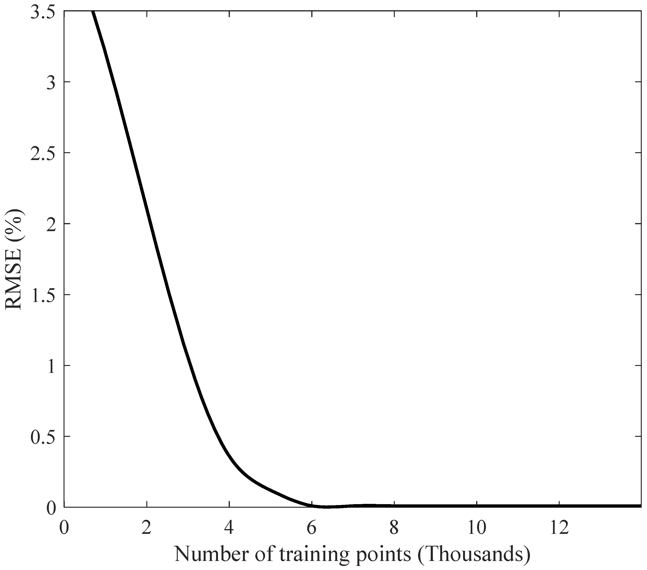
Figure 1. Power–time characteristics of energy storage systems.
Sustainability 17 02744 g001
Figure 2. The demand response classifications.
Sustainability 17 02744 g002
Figure 3. The schematic diagram of the proposed clean energy smart grid system.
Sustainability 17 02744 g003
Figure 4. The relationship between accumulated cycle count and depth of discharge for lithium-ion batteries.
Sustainability 17 02744 g004
Figure 5. The pumped hydroelectric energy storage schematic diagram.
Sustainability 17 02744 g005
Figure 6. Francis turbine efficiency and relative power.
Sustainability 17 02744 g006
Figure 7. The pseudo-code of the LEA algorithm used in this study.
Sustainability 17 02744 g007
Figure 8. The flowchart of sizing a clean energy smart grid system using the Nested lotus effect optimization algorithm.
Sustainability 17 02744 g008
Figure 9. The architecture of the artificial neural network used in this study.
Sustainability 17 02744 g009
Figure 10. The flowchart of sizing clean energy smart grid system using lotus effect optimization algorithm and artificial neural network.
Sustainability 17 02744 g010
Figure 11. Clean energy smart grid results without demand-side management.
Sustainability 17 02744 g011
Figure 12. Energy storage system operation without demand-side management.
Sustainability 17 02744 g012
Figure 13. Clean energy smart grid results with demand-side management at the −0.5 price elasticity of demand.
Sustainability 17 02744 g013
Figure 14. Energy storage system operation with demand-side management at the −0.5 price elasticity of demand.
Sustainability 17 02744 g014
Figure 15. The cost of different components of the clean energy smart grid system, with and without the demand-side management strategy.
Sustainability 17 02744 g015
Figure 16. The relationship between the root mean square error of the artificial neural network, along with the number of training points.
Sustainability 17 02744 g016
Table 3. The variation in the root mean square error (%), along with the number of training and testing points.
Training PointsTesting PointsRMSE (%)
100014,0003.2
200013,0002.1
300012,0001.05
400011,0000.36
500010,0000.12
600090000.01
700080000.01
800070000.01
900060000.01
10,00050000.01
11,00040000.01
12,00030000.01
13,00020000.01
14,00010000.01
Disclaimer/Publisher’s Note: The statements, opinions and data contained in all publications are solely those of the individual author(s) and contributor(s) and not of MDPI and/or the editor(s). MDPI and/or the editor(s) disclaim responsibility for any injury to people or property resulting from any ideas, methods, instructions or products referred to in the content.

